Exciton absorption spectra in narrow armchair graphene nanoribbons in electric fields

Abstract

We present an analytical investigation of the exciton optical absorption in a narrow armchair graphene nanoribbon (AGNR) in the presence of a longitudinal external electric field directed parallel to the ribbon axis. The two-body 2D Dirac equation for the massless electron and hole subject to the ribbon confinement, Coulomb interaction and electric field is employed. The ribbon confinement is assumed to be much stronger than the internal exciton electric field which in turn considerably exceeds the external electric field. This justifies an adiabatic approximation implying a slow longitudinal and fast transverse electron-hole relative motion governed by the exciton attraction and accompanied by the external electric field and ribbon confinement effects, respectively. In the single subband approximation of the isolated size-quantized subbands induced by the ribbon confinement the exciton electroabsorption coefficient is determined in an explicit form. The pronounced dependencies of the exciton peak positions, widths and intensities on the ribbon width and electric field strength are traced. The electron-hole exciton attraction modifies remarkably the Franz-Keldysh electroabsorption in the frequency region both below and above the edges determined by the size-quantized energy levels. In the double-subband approximation of the interacting ground and first excited subbands the combined effect of the exciton electro- and autoionization caused by the electric field and intersubband coupling, respectively, are explored. Our analytical results are in agreement with those obtained by numerical methods. Estimates of the expected experimental values for the typically employed AGNR show that for a weak electric field the exciton quasi-discrete states remain sufficiently stable to be observed in optical experiments, while relatively strong fields free the captured carriers to further restore their contribution to the transport.

1 Introduction

Following the early work in Ref. [1] especially during the last decade a large number of experimental and theoretical studies have been performed on the transport, electronic, and optical properties of armchair graphene nanoribbons (AGNR) (see [2, 3, 4, 5] and references therein). AGNR are spatially confined elongated strips of graphene monolayer. This is in particular due to the fact that in contrast to gapless unbound 2D graphene monolayers, AGNR are favorable for the formation of excitons (bound electron-hole pairs), which in turn strongly affect the 2D graphene electronic and optical properties. In 2D graphene the vanishing density of the electron and hole states at the Dirac points prevents the formation of excitons, while in the quasi-1D AGNR possessing an open band gap the bound exciton states can arise [6]. The existence of these states provides several reasons for the strong interest in AGNRs. The first reason is that AGNR being the interconnects between 2D graphene monolayers must support their ultrahigh carrier mobility in graphene-based nanoelectronic devices. At the same time the exciton effect, i.e. electron-hole attraction transforms free electrons and holes into neutral excitons and thereby suppresses the charge transport properties of graphene monolayers. Note that excitons in AGNR are bound much stronger than their counterparts in quasi-1D semiconductor structures, namely in the quantum wire (QWR) and in a bulk crystal subject to a strong magnetic field (diamagnetic excitons (DE)). The binding energies $E^{(\mbox{\tiny{b}})}$ of the excitons in the AGNR of width $d\simeq 1~{}\mbox{nm}$ reach the considerable value of $E^{(\mbox{\tiny{b}})}\simeq 1\,\mbox{eV}$ [7], while for realistic magnetic fields and QWR [8, 9] $E^{(\mbox{\tiny{b}})}\simeq 10-20\,\mbox{meV}$. Thus, the liberation mechanism for the AGNR charge carriers captured by the excitons is a relevant question of immediate interest.

In addition, the exciton effect changes drastically the optical properties of the AGNR. In particular, this is the absorption in the vicinity of the subband edges determined by the size-quantized electron-hole energy levels. The square-root divergency of the fundamental absorbtion profile specific for the quasi-1D structures is replaced by the finite value, associated with the peaks of the Rydberg series peaks broadening below each edge.

The second reason is that quasi-1D structures, namely DE [10], QWR [11] and AGNR [12] are favorable for the formation of not only strictly discrete but also metastable Fano resonances [13] like exciton states adjacent to the excited size-quantized energy levels. The nature of the Fano resonances lies in the inter-subband coupling between the discrete and low-lying continuous Rydberg states. Narrow AGNR outperform the mentioned 1D semiconductor structures in terms of the impact of the binding energy of the exciton states, their resonant energy widths and related parameters. The exciton binding energies and widths are proportional to the exciton Rydberg constant $Ry$ [12]. For the semiconductor structures the Rydberg constant does not depend on the confinement parameters, i.e. on the radius [11] and magnetic field [14] for the QWR and DE, respectively. For the AGNR with width $d$ we have $Ry\sim d^{-1}$ [15]. Thus, for narrow AGNRs dimensionality plays a crucial role and allows to control the relevant exciton properties.

External electric fields directed parallel to the graphene axis strongly affect the excitonic and related carrier mobility, the Fano resonances and optical absorption spectrum. The process of electric field ionization can be used as a tool for the release of the carriers bound within the strictly discrete and quasi-discrete exciton states and thereby enhance the conductance of both the AGNR and the nanoelectronic devices these ribbons are incorporated into. As established earlier for the bulk semiconductors, the electric fields act significantly on both the fundamental (Franz-Keldysh effect [16]) and exciton [17] absorption. They shift and broaden the discrete exciton peaks and modify remarkably the exciton spectrum both below [18] and above [19] the optical edge.

In addition, quasi-1D excitons in AGNR subject to electric fields allow us to study the process of exciton double channel ionization. The excited metastable exciton Rydberg series decay according to two channels: the autoionization channel, open due to the intersubband Fano coupling [10, 13], and the channel of electric field ionization, caused by under barrier tunneling [20].

Note that the majority of the theoretical approaches to the problem of the exciton in GNR are based on numerical calculations implying a considerable computational effort. The discrete part of the exciton absorption spectrum of GNR has been calculated numerically [7, 21, 22, 23] using density functional theory, employing the local density approximation, and the Bethe-Salpeter equation. Jia et al. [5] and Lu et al. [24] used the tight-binding approximation, while Alfonsi and Meneghetti [3] employed a full many-body exact diagonalization of a parametric Hubbard Hamiltonian in their calculations of the exciton peak positions and intensities. Gundra and Shukla [25] studied computationally the optical absorption in the zigzag GNR in the presence of electric fields. The Pariser-Parr-Pople-model Hamiltonian was employed, however the exciton effect was not taken into account. Only few works rely on analytical methods [2, 12, 15, 26], while many numerical studies of the electronic and optical properties of the GNR have been performed (see Ref. [25] and references therein). Numerical results are very helpful also for the detailed interpretation of a specific experiment. At the same time analytical approaches are appropriate to reveal the basic physics of the underlying phenomena especially at the first stages of the investigation. To our knowledge, analytical studies of the exciton electroabsorption in AGNR have not been performed in the literature yet.

In the present work, we develop an analytical approach to the problem of the exciton states in the narrow AGNR in the presence of an external electric fields directed parallel to the ribbon axis. The Coulomb electron-hole attraction is taken to be much weaker than the influence of the ribbon confinement and much stronger than the effect of the electric fields. The two-body 2D Dirac equation for the massless electron and hole in AGNR subject to the Coulomb and external electric fields is solved in the adiabatic approximation. This approximation implies that the transverse electron-hole motion governed by the ribbon confinement is much faster than the longitudinal motion controlled by the Coulomb and external electric fields. In the approximation of the isolated size-quantized subbands the optical absorption coefficient in the vicinity of the quasi discrete exciton states (peak positions, widths and intensities) and within the continuous band as a function of the ribbon width and electric field strength are determined explicitly. In the double-subband approximation the total widths of the first excited Rydberg series exciton peaks, associated with the electric field ionization and intersubband Fano coupling are investigated. Numerical estimates of the expected experimental values for realistic AGNR parameters and electric field strenghts are made. The aims of this work are to study the effect of the electric field and ribbon confinement on the exciton absorption spectrum and to elucidate the mechanism of the ionization process of the excitons yielding the increase of the carriers mobility in the AGNR. In addition, we intend to trigger further experimental and theoretical studies.

The paper is organized as follows. In Section 2 the general analytical equations are derived. The exciton electroabsorption coefficient is determined in the single- and double-subband approximations in Sections 3 and 4, respectively. A discussion of the obtained theoretical results and estimates of the expected experimental values is presented in Section 5. Section 6 contains our conclusions.

2 General approach

We consider the exciton optical absorption in electrically biased AGNR with width $d$ and length $L$ placed on the $x-y$ plane and bounded by straight lines $x=\pm d/2.$ The uniform electric field $\vec{F}$ as well as the polarization of the involved light wave are chosen to be parallel to the ribbon $y$-axis. The general approach to the problem of the exciton absorption is based on Refs. [27] and [28] devoted to the interband optical absorption in AGNR and exciton absorption in semiconductors, respectively. Since the mathematical details of this approach have been presented in Ref. [12] only an outline of our calculations will be provided below. The equation for the exciton absorption coefficient has the form

$$\alpha=\sum_{N}\alpha^{(N)};\quad\alpha^{(N)}=\frac{1}{n_{b}\varepsilon_{0}c}\sigma_{yy}^{(N)},$$ (1)

where $n_{b}$ is the refractive index of the ribbon substrate, $c$ is the speed of light, and $\sigma_{yy}^{(N)}$ is the component of the dynamical conductivity,

$$\sigma_{yy}^{(N)}=\frac{\pi p^{2}e^{2}}{\hbar S\Delta_{N}}\sum_{n,s}\big{|}\sigma^{(N)}_{xn(s)}\big{|}^{2}\delta\left(\hbar\omega-E_{Nn(s)}\right)\delta_{\vec{q}_{ph}\vec{K}}$$ (2)

determined by the matrix element

$$\sigma^{(N)}_{xn(s)}=\left<\vec{\Psi}^{(0)}(\vec{\rho}_{e},\vec{\rho}_{h})|\hat{\sigma}_{xh}\bigotimes\hat{I}_{e}+\hat{I}_{h}\bigotimes\hat{\sigma}_{xe}|\vec{\Psi}^{(\mbox{\tiny{x}})}_{Nn(s)}(\vec{\rho}_{e},\vec{\rho}_{h})\right>$$ (3)

of the Pauli matrix $\hat{\sigma}_{x}$ calculated between the ground state $\vec{\Psi}^{(0)}$ and exciton wave functions $\vec{\Psi}^{\mbox{\tiny(x)}}_{Nn(s)}$ of the bound $(n)$ and continuous $(s)$ states of the exciton, formed by an electron and hole related to size-quantized energy subbands with the common index $N$. The exciton states consisting of the electron and hole associated with the different $N_{e}\neq N_{h}$ subbands are optically inactive and can be excluded from expansion (8) (see justification in [29] and references therein). As usual, the symbol $\bigotimes$ denotes the tensor product of the Pauli $\hat{\sigma}_{x}$ and unit $\hat{I}$ matrices. In eq. (2) $p=\hbar v_{F}~{}(v_{F}=10^{6}\,\mbox{m/s})$ is the graphene energy parameter, $S=Ld$ is the area of the ribbon, $\Delta_{N}=2\varepsilon_{N}$ is the effective energy gap between the electron and hole subbands, branching from the size-quantized levels $\pm\varepsilon_{N}$ in the conduction and valence bands, respectively. The $\delta$-functions in eq. (2) reflect the conservation laws in the system formed by the absorbed photon with the energy $\hbar\omega$ and momentum $\hbar\vec{q}_{\mbox{\tiny{ph}}}$ plus the emersed exciton of the energy $E_{Nn(s)}$ and total momentum $\hbar\vec{K}$.

Following Elliot’s approach justified in detail in Ref. [28] the wave function $\vec{\Psi}^{(0)}$ of the ground state of the electron-hole pair in a semiconductor-like AGNR is chosen in the form

$$\vec{\Psi}^{(0)}(\vec{\rho}_{e},\vec{\rho}_{h})=\delta(y)\delta(x_{e}-x_{h})\left[\vec{\Phi}_{A}^{(0)}\bigotimes\vec{\Phi}_{A}^{(0)}+\vec{\Phi}_{B}^{(0)}\bigotimes\vec{\Phi}_{B}^{(0)}\right],$$ (4)

where $y=y_{e}-y_{h}$ is the relative $y$-coordinate and

$$\vec{\Phi}_{A}^{(0)}=\frac{1}{\sqrt{2}}\begin{array}[]{c}\begin{Bmatrix}-1\\ 0\\ 1\\ 0\end{Bmatrix}\end{array};\qquad\vec{\Phi}_{B}^{(0)}=\frac{1}{\sqrt{2}}\begin{array}[]{c}\begin{Bmatrix}0\\ 1\\ 0\\ -1\end{Bmatrix}\end{array}.$$

The exciton wave function $\vec{\Psi}^{\mbox{\tiny(x)}}$ obeys the equation

$$\hat{{\rm H}}_{\mbox{\tiny x}}\vec{\Psi}^{\mbox{\tiny(x)}}(\vec{\rho_{e}},\vec{\rho_{h}})=E\vec{\Psi}^{\mbox{\tiny(x)}}(\vec{\rho_{e}},\vec{\rho_{h}}).$$ (5)

In this equation

$$\hat{{\rm H}}_{\mbox{\tiny x}}=\hat{{\rm H}}_{h}(\hat{\vec{k}}_{h})\bigotimes\hat{I}_{e}+\hat{I}_{h}\bigotimes\hat{{\rm H}}_{e}(\hat{\vec{k}}_{e})+\hat{I}_{h}\bigotimes\hat{I}_{e}\left[V(\vec{\rho_{e}}-\vec{\rho_{h}})-eF(y_{e}-y_{h})\right]$$ (6)

is the traditional exciton Hamiltonian [30] formed by the electron and hole Hamiltonians $\hat{{\rm H}}_{j}(\hat{\vec{k}}_{j}),~{}j=e,h$ corresponding to the nonequivalent Dirac points
$\vec{K}^{(+,-)}=\pm K,0;~{}(K=4\pi/3a_{0},~{}a_{0}=2.46\,\mbox{{\AA}}$ is the graphene lattice constant) [31] and

$$V(\vec{\rho}_{e},\vec{\rho}_{h})=-\frac{e^{2}}{4\pi\varepsilon_{0}\epsilon_{\mbox{\tiny eff}}\sqrt{(x_{e}-x_{h})^{2}+(y_{e}-y_{h})^{2}}}.$$ (7)

is the 2D Coulomb potential of the electron-hole attraction. Here $\epsilon_{\mbox{\tiny eff}}=\frac{1}{2}(1+\epsilon+\pi q_{0})$ is the effective dielectric constant determined by the static dielectric constant $\epsilon$ of the substrate and by the parameter $q_{0}=e^{2}/4\pi\varepsilon_{0}p\simeq 2.2$ [15, 32].

Further we choose the exciton wave function $\vec{\Psi}^{\mbox{\tiny(x)}}$ in the form

$$\vec{\Psi}^{\mbox{\tiny(x)}}(\vec{\rho_{e}},\vec{\rho_{h}})=\frac{1}{\sqrt{2}}\sum_{N}\sum_{\alpha=A,B}u_{N\alpha}(y_{h})\vec{\Phi}_{N\alpha}(x_{h})\bigotimes\sum_{\beta=A,B}u_{N\beta}(y_{e})\vec{\Phi}_{N\beta}(x_{e}),$$ (8)

where $\vec{\Phi}_{NA(B)}(x_{e(h)})~{}\mbox{and}~{}u_{NA(B)}(y_{e(h)})$ are the wave functions describing the electron (hole) transverse $x-$ and longitudinal $y-$ states, governed by the ribbon confinement and exciton $V(\vec{\rho}_{e}-\vec{\rho}_{h})$ (7) and electric field $-eF(y_{e}-y_{h})$ potentials, respectively, in the $A(B)$ graphene sublattices. In equation (8) the sublattice wave functions $\vec{\Phi}_{NA,(B)}$ are as follows

$$\vec{\Phi}_{NA}(x_{j})=\begin{array}[]{c}\begin{Bmatrix}-\varphi_{N}(x_{j})\\ 0\\ \varphi_{N}^{\ast}(x_{j})\\ 0\end{Bmatrix}\end{array};\qquad\vec{\Phi}_{NB}(x_{j})=\begin{array}[]{c}\begin{Bmatrix}0\\ \varphi_{N}(x_{j})\\ 0\\ -\varphi_{N}^{\ast}(x_{j})\end{Bmatrix}\end{array},\quad j=e,h,$$

where the explicit form of the functions $\varphi_{N}(x_{j})$ is presented in Ref. [33]. The electron (hole) energies corresponding to the size-quantized transverse $N$ states are equal to $+(-)\varepsilon_{N}$ with

$$\varepsilon_{N}=|N-\tilde{\sigma}|\frac{\pi p}{d};~{}N=0,\pm 1,\pm 2,\ldots~{};\quad\tilde{\sigma}=\frac{Kd}{\pi}-\left[\frac{Kd}{\pi}\right].$$ (9)

Below, to be specific, we will consider AGNR of the family $\tilde{\sigma}=1/3$, providing a semiconductor-like gap structure.

Substituting the expansion of the wave function $\vec{\Psi}^{\mbox{\tiny(x)}}(\vec{\rho_{e}},\vec{\rho_{h}})$ over the ortho-normalized basis set $\vec{\Phi}_{N\alpha}(x_{h})\bigotimes\vec{\Phi}_{N\beta}(x_{e})$ (8) into eq. (5) and in view of the equations

$$\hat{H}_{j}(\hat{\vec{k_{j}}})\vec{\Phi}_{NA(B)}(x_{j})=\varepsilon_{N}\vec{\Phi}_{NB(A)}(x_{j})$$

we arrive after routine manipulations to the set of the equations for the expansion coefficients $u_{N\alpha}(y_{h})u_{N\beta}(y_{e})$ (see eq. (14) in Ref. [12]) written in terms of the centre of mass $Y=\frac{1}{2}(y_{e}+y_{h})$ and relative $y=y_{e}-y_{h}$ coordinates

$$u_{N\alpha}(y_{h})u_{N\beta}(y_{e})=\frac{{\rm e}^{{\rm i}QY}}{\sqrt{L}}\xi_{N\alpha\beta}(y)~{};\,\xi_{NAA}=\xi_{N1}~{};\,\xi_{NAB,(BA)}=\frac{1}{\sqrt{2}}(\xi_{N2}\pm\xi_{N3})~{};\,\xi_{NBB}=\xi_{N4};$$

$\hbar Q$ is the longitudinal component of the exciton total momentum.

Further this set is solved in the adiabatic approximation. This implies that the fast transverse $x$- and slow $y$- motions affected by the ribbon confinement and exciton attraction plus weak electric field, respectively, are adiabatically separated. The adiabaticity parameter $q$ i.e. the Coulomb potential strength (7) scaled with the graphene energetic parameter $p$ and the imposed adiabatic condition are as follows

$$q=\frac{e^{2}}{4\pi\varepsilon_{0}\epsilon_{\mbox{\tiny eff}}p};\quad q<<1.$$ (10)

Under this condition the set for the functions $\xi_{Nj},~{}j=1,2,3,4.$ [12] transforms into that for the functions $\xi_{N1}=\xi_{N4}=\frac{1}{\sqrt{2}}\xi_{N2}\equiv\xi_{N},~{}\xi_{N3}\ll\xi_{N1}$

$$-\frac{\hbar^{2}}{2\mu_{N}}\xi_{N}^{{}^{\prime\prime}}(y)+\left[V_{NN}(y)-eFy-W_{N}\right]\xi_{N}(y)+\sum_{N^{\prime}\neq N}V_{N^{\prime}N}(y)\xi_{N^{\prime}}(y)=0.$$ (11)

These equations describe the relative motion of the 1D exciton with centre-of-mass momentum $Q=0$, reduced mass $\mu_{N}=\frac{\hbar^{2}\Delta_{N}}{4p^{2}}$ and energy $W_{N}=E-\Delta_{N}$ in the presence of the external electric $-eFy$ and quasi-Coulomb $V_{N^{\prime}N}(y)$ potentials, where

$$V_{N^{\prime}N}(y)=\frac{1}{d^{2}}\int_{-\frac{d}{2}}^{+\frac{d}{2}}dx_{e}\int_{-\frac{d}{2}}^{+\frac{d}{2}}dx_{h}V(\vec{\rho})\cos\left[(N-N^{\prime})\pi\left(\frac{x_{e}}{d}-\frac{1}{2}\right)\right]$$ (12)

$$\times\cos\left[(N-N^{\prime})\pi\left(\frac{x_{h}}{d}-\frac{1}{2}\right)\right]~{};\,\vec{\rho}=\vec{\rho}_{e}-\vec{\rho}_{h}~{},$$

determined by eq. (7) for the potential $V(\vec{\rho})$ with

$$V_{N^{\prime}N}(y)=-\frac{\beta}{|y|}\left[\delta_{N^{\prime}N}+O\left(\frac{d^{2}}{y^{2}}\right)\delta_{|N^{\prime}-N|(2s+1)}\right]~{};\,s=0,1,2,\ldots;~{}\mbox{at}~{}|y|\gg d.$$ (13)

Other parameters related to the $N$th subband are the exciton Bohr radius $a_{N}=\frac{4\pi\varepsilon_{0}\epsilon_{\mbox{\tiny eff}}\hbar^{2}}{\mu_{N}e^{2}}$, exciton Rydberg constant $Ry_{N}=\frac{\hbar^{2}}{2\mu_{N}a_{N}^{2}}(=\frac{\Delta_{N}q^{2}}{8})$ and dimensionless electric field $f_{N}=\frac{F}{F_{N}}$, which is the external electric field $F$ scaled with the exciton electric field $F_{N}=\frac{Ry_{N}}{ea_{N}}$.

Using eqs. (4) and (8) for the ground state $\vec{\Psi}^{(0)}$ and exciton $\vec{\Psi}^{(\tiny x)}$ wave functions, respectively, we determine the matrix element (3) of the dipole exciton optical transition in the form $\sigma_{xn(s)}^{(N)}=-\sqrt{L}\xi_{N}(0)$. As expected, for the noninteracting electron-hole pair for which $\xi_{N}(y)=\frac{1}{\sqrt{L}}\exp^{{\rm i}sy}$ the matrix element of the fundamental optical transition reads $|\sigma_{xn(s)}^{(N)}|=1$ [27]. The contribution $\alpha^{(N)}$ (see eqs. (1), (2)) to the coefficient of the exciton absorption $\alpha$ in the vicinity of the edge $\Delta_{N}$ takes on the following appearence

$$\alpha_{N}(\omega)=\alpha^{(0)}\frac{4\pi p^{2}}{n_{b}\Delta_{N}d}\sum_{n(s)}\big{|}\xi_{N1}(0)\big{|}^{2}\delta\left(\hbar\omega-E_{Nn(s)}\right),$$ (14)

where $\alpha^{(0)}=e^{2}/4\varepsilon_{0}\hbar c\simeq 2.3\cdot 10^{-2}$ is the absorption of the suspended graphene. As mentioned above the details of the calculations of eq. (14) including the explicit forms of the Hamiltonians $\hat{H}_{e,h}(\hat{\vec{k}}_{e,h})$ in eq. (6), sublattice wave functions $\vec{\Phi}_{NA,(B)}(x)$ in eq. (8) and set of functions $\chi_{N1}-\chi_{N4}$ can be found in Ref. [12].

3 Spectrum of the exciton electroabsorption: Single-subband approximation

Here we employ the single-subband approximation ignoring the coupling between the electron-hole subbands with the different indices $N$. It follows from eq. (13) that in the narrow ribbon with small width $d$ the diagonal potentials $V_{NN}$ dominate the off-diagonal ones in the set of equations (11). This allows us to set $V_{N^{\prime}N}=V_{N}\delta_{N^{\prime}N}$, omit the $\Sigma_{N^{\prime}}$ from eqs. (11) and arrive at the equations for the functions $\chi_{N}(y)$ governed by the diagonal Coulomb contribution

$$V_{N}(y)=\frac{2}{d}qp\left[\ln\frac{\frac{|y|}{d}}{1+\sqrt{1+\frac{y^{2}}{d^{2}}}}+\sqrt{1+\frac{y^{2}}{d^{2}}}-\frac{|y|}{d}\right]=\left\{\begin{array}[]{cl}\frac{qp}{d}\ln\frac{y^{2}}{d^{2}}~{};&\frac{|y|}{d}\ll 1\\ -\frac{qp}{|y|}~{};&\frac{|y|}{d}\gg 1\end{array}\right.$$ (17)

and the electric field potential $-eFy$.

These equations are solved by matching in the intermediate regions the wave functions valid in the inner $0\leq\mid y\mid\ll a_{N}$, Coulomb $d\ll\mid y\mid\ll(\mid y_{N}\mid a_{N})^{\frac{1}{2}}$ and ”electric” $\mid y\mid\gg(\mid y_{N}\mid a_{N})^{\frac{1}{2}}$ regions, determined by the exciton Bohr radius $a_{N}$ and turning point $y_{N}=-\frac{W_{N}}{eF}$ for vanishing classical momentum $\mathscr{P}(y)=\sqrt{2\mu_{N}\left(W_{N}+eFy\right)}$. In the inner and Coulomb regions the exciton electric field $F_{N}$ considerably exceeds the external electric field $F$, while in the ”electric” region the exciton potentials $V_{N}(y)$ can be treated as a small perturbation to the external field effects. The exciton absorption coefficient is determined for the photon energies $\hbar\omega=E$ below the absorption edge $0>\hbar\omega-\Delta_{N}\simeq-\frac{Ry_{N}}{n^{2}},~{}n\simeq 0,1,2,\ldots$ close to the energies of the bound Rydberg states, for the frequencies $\hbar\omega-\Delta_{N}<0$ positioned far away from the $Nn$ exciton peaks and for the frequency region above the edge $\hbar\omega-\Delta_{N}>0.$ The approach presented in this section closely resembles those in the works [11, 34] dedicated to the exciton electroabsorption in QWR and impurity states in AGNR subject to electric fields, respectively. Here we focus only on the main features leaving aside the details.

3.1 Frequency region $\hbar\omega-\Delta_{N}<0$

At this stage it is convenient to introduce the exciton quantum number $\kappa_{N}$ and reciprocal length $\nu_{N}$ defined by $W_{N}=-Ry_{N}/\kappa_{N}^{2}$ and $\nu_{N}=2(\kappa_{N}a_{N})^{-1}$, respectively. In the inner region an iteration method is employed. Double integration of eq. (11) without the term involving $\sum_{N^{\prime}\neq N}$ with the trial function and its derivative $\xi_{N}^{(0)}(y)=c_{N},~{}\xi_{N}^{(0)^{\prime}}(y)=0$ relevant to the optically active excitons (see eq. (14) ) generates the function

$$\xi_{N}(y)=c_{N}\left[1-2\frac{y}{a_{N}}\left(\ln\frac{2y}{d}-\frac{1}{2}\right)\right].$$ (18)

In the Coulomb region the general solution to eq. (11)

$$\xi_{N}(y)=A_{N}W_{\kappa_{N},\frac{1}{2}}(\tau)+B_{N}M_{\kappa_{N},\frac{1}{2}}(\tau),~{}\tau=\nu_{N}y$$ (19)

can be written in terms of the Whittaker functions $W_{\kappa_{N},\frac{1}{2}}~{}\mbox{and}~{}M_{\kappa_{N},\frac{1}{2}}$ [35]. In the ”electric” region eq. (11) reads

$$\xi_{N}^{{}^{\prime\prime}}(x)-G_{N}(x)\xi_{N}(x)=0,$$ (20)

where

$$G_{N}(x)=x+\frac{2f_{N}^{-\frac{1}{3}}}{x-\kappa_{N}^{-2}f_{N}^{-\frac{2}{3}}};~{}x=-\frac{y}{b_{N}}+\kappa_{N}^{-2}f_{N}^{-\frac{2}{3}};~{}b_{N}(F)=\left(\frac{\hbar^{2}}{2\mu_{N}eF}\right)^{\frac{1}{3}}.$$

Following the comparison equation method [36] the general solution normalized according to $\delta(W_{N}-W_{N}^{\prime})$

$$\xi_{N}(y)=\tilde{C}_{N}\frac{\left[\frac{3}{2}S_{N}(x)\right]^{\frac{1}{6}}}{G_{N}(x)^{\frac{1}{4}}}\left\{\sin\vartheta_{N}Ai\left[\left(\frac{3}{2}S_{N}(x)\right)^{\frac{2}{3}}\right]+\cos\vartheta_{N}Bi\left[\left(\frac{3}{2}S_{N}(x)\right)^{\frac{2}{3}}\right]\right\}$$ (21)

is written in terms of the Airy functions $Ai$ and $Bi$ [35]. In eq. (21)

$$S_{N}(x)=\int_{0}^{x}G_{N}^{\frac{1}{2}}(u)du,\quad\tilde{C}_{N}^{2}=\frac{1}{\mathscr{E}_{N}b_{N}},\quad\mathscr{E}_{N}(F)=\frac{\hbar^{2}}{2\mu_{N}b_{N}^{2}},$$

and $\vartheta_{N}$ is an arbitrary phase.

A comparison of function (18) and (19) for $\tau\ll 1$ and then the asymptotic expansions of functions (19) for $\tau\gg 1$ and (21) for $S\gg 1$ [35] lead to the set of equations

$$c_{N}-\frac{A_{N}}{\Gamma(1-\kappa_{N})}=0;$$ (22)

$$A_{N}Y_{N}(\kappa_{N})+B_{N}\Gamma(-\kappa_{N})=0;$$ (23)

$$A_{N}-B_{N}\frac{\cos\pi\kappa_{N}}{\Gamma(1+\kappa_{N})}-\tilde{C}_{N}\pi^{-\frac{1}{2}}\kappa_{N}^{\frac{1}{2}}f_{N}^{\frac{1}{6}}\cos\vartheta_{N}\Omega_{N}^{-1}=0;$$ (24)

$$B_{N}\frac{1}{\Gamma(1-\kappa_{N})}-\tilde{C}_{N}\frac{1}{2}\pi^{-\frac{1}{2}}\kappa_{N}^{\frac{1}{2}}f_{N}^{\frac{1}{6}}\sin\vartheta_{N}\Omega_{N}=0.$$ (25)

In this set

$$Y_{N}(\kappa_{N})=\pi\cot\pi\kappa_{N}-\frac{1}{2\kappa_{N}}-\ln\kappa_{N}+\psi(1+\kappa_{N})+\ln q+\ln\frac{\mid N-\tilde{\sigma}\mid\pi}{2}+2C-\frac{1}{2},$$ (26)

where $C=0.577$ is the Euler constant, $\psi(1+\kappa_{N})$ is the logarithmic derivative of the $\Gamma$ function,

$$\Omega_{N}=\exp\left\{-\frac{2}{3f_{N}\kappa_{N}^{3}}+\kappa_{N}\ln\frac{8}{f_{N}\kappa_{N}^{3}}\right\}.$$ (27)

Solving the set of equations (22)-(25) with respect to the coefficients $c_{N},A_{N},B_{N},\tilde{C}_{N}$ by the determinantal method, we determine the phase $\vartheta_{N}$ and then the coefficient $c_{N}^{2}=\xi_{N}^{2}(0)$

$$c_{N}^{2}=\frac{1}{2\pi pq}\frac{\kappa_{N}\Gamma^{2}(-\kappa_{N})}{Y^{2}(\kappa_{N})}\Omega_{N}^{2}\left\{1+\frac{\Omega_{N}^{4}\Gamma^{4}(1-\kappa_{N})}{4\kappa_{N}^{2}}\left[\frac{1}{Y_{N}(\kappa_{N})}-\frac{\sin 2\pi\kappa_{N}}{2\pi}\right]^{2}\right\}^{-1}$$ (28)

which provides us with the absorption coefficient (14) $\alpha_{N}=\alpha^{(0)}\frac{2p}{n_{b}\mid N-\tilde{\sigma}\mid}c_{N}^{2}$. The obtained results are valid under the condition  $f_{N}\kappa_{N}^{3}\ll 1$, resulting in  $\Omega_{N}\ll 1$.

3.1.1 Exciton electroabsorption

Expanding function (26) in the vicinity of the discrete exciton energies, specified by the quantum numbers $\kappa_{Nn}$ calculated from equation

$$Y_{N}(\kappa_{Nn})=0;~{}\kappa_{Nn}=n+\beta_{Nn};~{}\beta_{Nn}<1;~{}n=0,1,2,\ldots,$$ (29)

eq. (28) is rearranged to

$$c_{Nn}^{2}=\frac{q\Delta_{N}}{4p\kappa_{Nn}^{3}\mid\frac{\partial Y_{N}}{\partial\kappa_{Nn}}\mid}\Lambda_{Nn}\left(W_{N}\right);\quad\frac{\partial Y_{N}}{\partial\kappa_{Nn}}=\left\{\begin{array}[]{ll}-(2\kappa_{Nn}^{2})^{-1},\,n=0;\,\kappa_{Nn}=\beta_{N0};\\ -\beta_{Nn}^{-2},\,n=1,2,\ldots;\,\kappa_{Nn}=n+\beta_{Nn},\end{array}\right.$$ (32)

where the function $\Lambda_{Nn}\left(W_{N}\right)$ describing the Lorentzian form of the optical absorption peak reads

$$\Lambda_{Nn}(W_{N})=\frac{\Gamma_{Nn}^{\left(\mbox{\tiny{el}}\right)}}{2\pi\left\{\left[W_{N}-W_{Nn}-\Delta W_{Nn}^{(r)}\right]^{2}+\frac{\Gamma_{Nn}^{\left(\mbox{\tiny{el}}\right)2}}{4}\right\}};~{}W_{N}=\hbar\omega-\Delta_{N}.$$ (33)

In eq. (33) $W_{Nn}=-Ry_{N}(n+\beta_{Nn})^{-2},\quad\Gamma_{Nn}^{\left(\mbox{\tiny{el}}\right)}~{}\mbox{and}~{}\Delta W_{Nn}^{(r)}\sim\Gamma_{Nn}^{\left(\mbox{\tiny{el}}\right)}\Omega_{N}^{2}\beta_{Nn}^{-1}\ll\Gamma_{Nn}^{\left(\mbox{\tiny{el}}\right)}$ are the exciton energy levels in the absence of the electric field counted from the energy gap $\Delta_{N}$ and the resonant widths and shifts of the optical peaks, respectively, caused by the electric field ionization of the exciton states. We have omitted here the negligibly small Stark corrections to the energies $W_{Nn}$ caused by the weak electric fields (see Sec. 5, subsec. 5.1.1) and further ignore the resonant shifts $\Delta W_{Nn}^{(r)}$. The reasons for the latter approximation are as follows: (i) the shifts are much smaller than the corresponding widths and (ii) they do not change the form of the exciton spectrum. The widths $\Gamma_{Nn}^{\left(\mbox{\tiny{el}}\right)}$ transform the $\delta$-function peaks in an unbiased AGNR [12] into the maxima of finite width $\Gamma_{Nn}^{\left(\mbox{\tiny{el}}\right)}$.

An explicit form of the width $\Gamma_{Nn}^{\left(\mbox{\tiny{el}}\right)}$ and maximum of the absorption coefficient $c_{Nn}^{2(\mbox{\tiny{max}})}$ determined by eqs. (28) and (32), respectively, are as follows

$$\Gamma_{Nn}^{\left(\mbox{\tiny{el}}\right)}=2(1+\delta_{n0})\frac{Ry_{N}\Omega_{N}^{2}}{\kappa_{Nn}^{2}\Gamma^{2}(1+\kappa_{Nn})},\quad c_{Nn}^{2(\mbox{\tiny{max}})}=\frac{2\beta_{Nn}^{2}\Gamma^{2}(1+\kappa_{Nn})}{\pi pq\kappa_{Nn}\Omega_{N}^{2}},$$ (34)

where $\delta_{n0}$ is the Kronecker symbol. The quantum defects $\beta_{Nn}~{}\mbox{and factor}~{}\Omega_{N}$ can be found from eqs. (29) and (27), respectively. As expected, in the absence of the electric fields $F=0,~{}\Omega_{N}=0$ eqs. (32) and (33) transform into those describing the $\delta$-function type exciton peaks in an electrically unbiased AGNR [12]. In principle, the resonant widths $\Gamma_{Nn}^{\left(\mbox{\tiny{el}}\right)}$ and shifts $\Delta W_{Nn}\sim\frac{\Omega_{Nn}^{2}}{\beta_{Nn}}\Gamma_{Nn}^{\left(\mbox{\tiny{el}}\right)}$ of the exciton peaks can be found as the imaginary components of the complex energies of the quasi-discrete $Nn$ states [34]. These states are relevant to the poles of the scattering matrix $S(\vartheta_{N})=\exp(2{\rm i}\vartheta_{N})$ [37]. Setting in the set of eqs. (22)-(25) $\cot\vartheta_{N}={\rm i}$ and then solving this set by the determinantal method we find the complex quantum numbers $\kappa_{Nn}$ and the complex energies $W_{N}=W_{Nn}+\Delta W_{Nn}-\frac{{\rm i}}{2}\Gamma_{Nn}^{\left(\mbox{\tiny{el}}\right)}$ comprising the unperturbed Rydberg levels $W_{Nn}=-Ry_{N}/\kappa_{Nn}^{2}$, resonant width $\Gamma_{Nn}^{\left(\mbox{\tiny{el}}\right)}$ (34) and shift $\Delta W_{Nn}\sim\frac{\Omega_{Nn}^{2}}{\delta_{Nn}}\Gamma_{Nn}^{\left(\mbox{\tiny{el}}\right)}$.

3.1.2 Franz-Keldysh exciton absorption

Here we consider the frequencies $\hbar\omega<\Delta_{N}$, positioned away from the quasi-discrete exciton $Nn$ peaks. It allows us to neglect in eq. (28) the small term $\sim\Omega_{N}^{4}\Gamma^{4}(1-\kappa_{N})\kappa_{N}^{-2}$. This equation becomes

$$c_{N}^{2}=c_{N(\mbox{\tiny{F-K}})}^{2}T_{N}$$ (35)

, where

$$c_{N(\mbox{\tiny{F-K}})}^{2}=\frac{1}{\sqrt{2}\pi p}\left(\frac{\Delta_{N}-\hbar\omega}{\Delta_{N}}\right)^{-\frac{1}{2}}\exp\left\{-\frac{4}{3}\left(\frac{1}{f_{N}\kappa_{N}^{3}}\right)^{\frac{3}{2}}\right\}$$ (36)

is the electroabsorption coefficient in the AGNR associated with the photon-assisted inter-subband tunneling of the free carriers (F-K effect [16]) and

$$T_{N}=\frac{\Gamma^{2}(-\kappa_{N})}{4Y_{N}^{2}(\kappa_{N})}\exp\left\{2\kappa_{N}\ln\frac{8}{f_{N}\kappa_{N}^{3}}\right\}$$ (37)

is the factor describing the exciton influence on the F-K absorption. The equations (35-37) are derived for the frequency shift $\Delta_{N}-\hbar\omega$ significantly exceeding the energy $\mathscr{E}_{N}\,(f_{N}\kappa_{N}^{3}\ll 1)$. As expected, in the absence of the exciton effect $(\kappa_{N}\rightarrow 0)\,~{}\Gamma(-\kappa_{N})^{2}=4Y(\kappa_{N}^{2}),~{}T_{N}(\kappa_{N})=1\,\mbox{and}\,c_{N}^{2}=c_{N(\mbox{\tiny{F-K}})}^{2}$. For the zeroth electric fields $F=0$ the coefficient $c_{N(\mbox{\tiny{F-K}})}^{2}=0$ which in turn leads to the zeroth absorption $c_{N}^{2}=0$ for the frequencies distant from the exciton peaks.

3.2 Frequency region $\hbar\omega-\Delta_{N}>0$

For these energies we introduce the quantum number $\zeta_{N}$ and parameter $s_{N}$ defined by $W_{N}=Ry_{N}\zeta^{-2}$ and $s_{N}=2(\zeta_{N}a_{N})^{-1}$, respectively. In the Coulomb region the general solution to eq. (11) has the form

$$\xi_{N}(y)=D_{N}\left[e^{{\rm i}\Theta_{N}}W_{{\rm i}\zeta_{N},\frac{1}{2}}(t)+e^{-{\rm i}\Theta_{N}}W_{-{\rm i}\zeta_{N},\frac{1}{2}}(-t)\right];~{}t=-{\rm i}s_{N}y,$$ (38)

where $\Theta_{N}$ is an arbitrary phase.

In the ”electric” region equation (11) reads

$$\xi_{N}^{{}^{\prime\prime}}(x)-\tilde{G}_{N}(x)\xi_{N}(x)=0,$$ (39)

where

$$\tilde{G}_{N}(x)=x+\frac{2f_{N}^{-\frac{1}{3}}}{x+\zeta_{N}^{-2}f_{N}^{-\frac{2}{3}}};~{}x=-\frac{y}{b_{N}}-\zeta_{N}^{-2}f_{N}^{-\frac{2}{3}}$$

with the general solution

$$\xi_{N}(y)=\tilde{C}_{N}\frac{\left[\frac{3}{2}\tilde{S}_{N}(x)\right]^{\frac{1}{6}}}{\tilde{G}_{N}(x)^{\frac{1}{4}}}Ai\left[\left(\frac{3}{2}\tilde{S}_{N}(x)\right)^{\frac{2}{3}}\right],$$ (40)

decreasing towards the region $y\ll y_{N}~{}(y_{N}<0)$ and normalized according to $\delta\left(W_{N}-W_{N}^{{}^{\prime}}\right)$. In eq. (40)

$$\tilde{S}_{N}(x)=\int_{0}^{x}\tilde{G}_{N}(u)du$$

and $\tilde{C}_{N}$ is the same as that in eq. (21).

A comparison of functions (18) and (38) within the inner region and then the asymptotic expansions of functions (38) and (40) for $\mid t\mid\gg 1$ and $\tilde{S}_{N}\gg 1$, respectively, lead to the set of equations

$$c_{N}=-2D_{N}\left(\frac{\sinh\pi\zeta_{N}}{\pi\zeta_{N}}\right)^{\frac{1}{2}}\sin\left(\Theta_{N}+\sigma_{N}\right),\quad\sigma_{N}=\mbox{arg}\Gamma({\rm i}\zeta_{N}),$$ (41)

$$2D_{N}{\rm e}^{\frac{\pi\zeta_{N}}{2}}=\tilde{C}_{N}\pi^{-\frac{1}{2}}\zeta_{N}^{\frac{1}{2}}f_{N}^{\frac{1}{6}},$$ (42)

$$\Theta_{N}=\frac{2}{3f_{N}\zeta_{N}^{3}}-\zeta_{N}\ln\frac{8}{f_{N}\zeta_{N}^{3}}-\frac{\pi}{4}.$$ (43)

This set results in the coefficient $c_{N}=\xi_{N}(0)$ with

$$c_{N}^{2}=\frac{1}{\pi p}\left(\frac{\Delta_{N}}{\hbar\omega-\Delta_{N}}\right)^{\frac{1}{2}}Z_{N}\sin^{2}\left(\frac{2}{3f_{N}\zeta_{N}^{3}}+\frac{\pi}{4}+\Delta\Theta_{NZ}\right)$$ (44)

totally determining the absorption coefficient (14) $\alpha_{N}=\alpha^{(0)}\frac{2p}{n_{b}\mid N-\tilde{\sigma}\mid}c_{N}^{2}$ in the frequency region $\hbar\omega-\Delta_{N}>0$.

The Sommerfeld factor $Z_{N}$ and phase shift $\Delta\Theta_{NZ}$ both responsible for the influence of the exciton on the F-K absorption associated with the unbound electron-hole pair are given by

$$Z_{N}={\rm e}^{-\pi\zeta_{N}}\frac{\sinh\pi\zeta_{N}}{\pi\zeta_{N}}~{}\mbox{and}~{}\Delta\Theta_{NZ}=-\zeta_{N}\ln\frac{8}{f_{N}\zeta_{N}^{3}}-\frac{\pi}{2}+\sigma_{N},$$ (45)

respectively. Eqs. (44) and (45) are valid for frequency shifts from the edge by an amount $\hbar\omega-\Delta_{N}$ considerably exceeding the energy $\mathscr{E}\,(f_{N}\zeta_{N}^{3}\ll 1)$. In the absence of the exciton effect $(\zeta_{N}\rightarrow 0)$ we arrive at the Sommerfeld factor $Z_{N}=1$ and phase shift $\Delta\Theta_{NZ}=-\pi$. This transforms eq. (44) into that for the F-K oscillations. In the case of a vanishing electric field $F=0$ the rapidly oscillating function transforms into 1/2 and we obtain the coefficient $c_{N}^{2}$ in eq. (44) for the exciton absorption in the continuous spectrum region [12].

4 Spectrum of the exciton electroabsorption: Double-subband approximation

In this section we consider the influence of the coupling between the continuous and discrete states emanating from the ground $\Delta_{0}$ and adjacent to the first excited $\Delta_{1}$ size-quantized energy levels, respectively. We focus on the exciton electroabsorbtion in the frequency region $\Delta_{0}<\hbar\omega<\Delta_{1}$ in the vicinity of the resonant peaks $\hbar\omega-\Delta_{1}=-Ry_{1}/\kappa_{1n}^{2}.$ The common resonant energy $E=\hbar\omega$ of the interacting states is

$$E=\Delta_{1}-\frac{Ry_{1}}{\kappa_{1}^{2}}=\Delta_{0}+\frac{Ry_{0}}{\zeta_{0}^{2}}.$$ (46)

The corresponding two-fold set of equations follows from the general one (11) limited to $N,N^{\prime}=0,1$. To avoid routine and cumbersome calculations only an outline of the mathematical procedure will be given below. The needed details can be found in works in which the problems of the exciton electroabsorption in QWR [11] and impurity states in electrically biased AGNR [34] have been studied. Using the trial functions and its derivatives $\xi_{1}^{(0)}(y)=c_{1},\xi_{0}^{(0)}(y)=c_{0},\xi_{1}^{(0)^{\prime}}(y)=0,\xi_{0}^{(0)^{\prime}}(y)=0$ and double integrating the two-fold set we arrive at the functions $\xi_{1}(y)~{}\mbox{and}~{}\xi_{0}(y)$ valid in the inner regions $d\ll y\ll\kappa_{1}a_{1}~{}\mbox{and}~{}d\ll y\ll\zeta_{0}a_{0}$. Matching these functions with the functions (19) for $\tau\ll 1,N=1$ and (38) for $\mid t\mid\ \ll 1,N=0$, respectively, we obtain

$$\frac{A_{1}}{\Gamma(-\kappa_{1})}+\kappa_{1}c_{1}=0,$$ (47)

$$\frac{A_{1}}{\Gamma(-\kappa_{1})}Y_{1}(\kappa_{1})+B_{1}-\kappa_{1}\gamma_{01}c_{0}=0,$$ (48)

$$c_{0}+2D_{0}\left(\frac{\sinh\pi\zeta_{0}}{\pi\zeta_{0}}\right)^{\frac{1}{2}}\sin\left(\Theta_{0}+\sigma_{0}\right)=0,$$ (49)

$$c_{0}\eta_{0}(\zeta_{0})+\gamma_{01}c_{1}=0.$$ (50)

In these equations

$$\eta_{0}(\zeta_{0})=\lambda_{0}(\zeta_{0})-\frac{\pi}{1-\rm e^{-2\pi\zeta_{0}}}\cot\left(\Theta_{0}+\sigma_{0}\right);\quad\sigma_{0}=\mbox{arg}\Gamma({\rm i}\zeta_{0});$$

$$\lambda_{0}(\zeta_{0})=\frac{1}{2}[\psi(1+{\rm i}\zeta_{0})+\psi(1-{\rm i}\zeta_{0})]-\ln\zeta_{0}+\ln\frac{\mid\tilde{\sigma}\mid\pi}{2}+2C-\frac{1}{2}+\ln q.$$ (51)

The parameter

$$\gamma_{01}=\frac{1}{2d^{2}}\int_{-\frac{d}{2}}^{\frac{d}{2}}dx_{e}\int_{-\frac{d}{2}}^{\frac{d}{2}}dx_{h}\ln\mid x_{e}-x_{h}\mid\sin\frac{\pi}{d}x_{e}\sin\frac{\pi}{d}x_{h}=0.387$$

describes the coupling induced by the off-diagonal potentials $V_{10}=V_{01}$ (12). The function $Y_{1}(\kappa_{1})$ is given by eq. (26) for $N=1$.

Comparing functions (19) for $\tau\gg 1$ and (21) for $S\gg 1$ both for $N=1$ we obtain equations (24) and (25) both for $N=1$. The relationship between the phases $\vartheta_{1}$ and $\Theta_{0}$ is derived by equating the phases in the asymptotic expansions of functions (21) for $S\gg 1$ and (38) for $\mid t\mid\gg 1$ to give

$$\Theta_{0}+\sigma_{0}=-\vartheta_{1}+\frac{2}{3f_{1}\kappa_{1}^{3}}-\kappa_{1}\ln\frac{8}{f_{1}\kappa_{1}^{3}}-\frac{\pi}{4}.$$ (52)

Solving the set of eqs. (47)-(50) and (24), (25) for $N=1$ with respect to the coefficients $c_{0},c_{1},A_{1},B_{1},D_{0},\tilde{C}_{1}$ by the determinantal method, we obtain the equation containing the phase $\vartheta_{1}$ and $\Theta_{0}+\sigma_{0}$ linked by eq. (52)

$$\eta_{0}(\Theta_{0})\left\{Y_{1}(\kappa_{1})-\left[\frac{\sin 2\pi\kappa_{1}}{2\pi}+\frac{2\cot\vartheta_{1}}{\kappa_{1}\Gamma^{2}(-\kappa_{1})\Omega_{1}^{2}}\right]^{-1}\right\}-\gamma_{01}^{2}=0.$$ (53)

As expected, the just derived set of equations and eq. (53) satisfy the limiting transitions. In the single subband approximations neglecting the coupling parameter $\gamma_{01}$, eq. (53) decomposes into two ones. Determining $\cot\vartheta_{1}$, by setting to zero the curly bracket we arrive at the absorption coefficient $\alpha_{1}\sim c_{1}^{2}$ (28) describing the exciton electroabsorption in the frequency region $\hbar\omega<\Delta_{1}$. For a vanishing electric field $F=0,~{}\Omega_{1}=0$ eq. (53) generates the equation $\eta_{0}=\gamma_{01}^{2}Y_{1}^{-1}$ that in turn allows us to determine $\cot(\Theta_{0}+\sigma_{0})$. Using eqs. (47)-(50) with $B_{1}=0$ and $D_{0}=(4\pi pq)^{-1/2}\zeta_{0}^{1/2}\rm e^{-\pi\zeta_{0}/2}$ providing the normalization of function (38) to $\delta(W_{0}-W_{0}^{\prime})$ we arrive to the absorption coefficient $\alpha_{1}\sim(c_{1}+c_{0})^{2}$. This coefficient is determined by eqs. (32) and (33) in which the resonant width $\Gamma_{1n}^{\left(\mbox{\tiny{el}}\right)}$ and corresponding resonant shift are replaced by the Fano resonant width $\Gamma_{1n}^{\left(\mbox{\tiny{F}}\right)}$ and shift $\sim q^{3}\Gamma_{1n}^{\left(\mbox{\tiny{F}}\right)}$. The latter have been calculated in Ref. [12] to give

$$\Gamma_{1n}^{\left(\mbox{\tiny{F}}\right)}=\frac{8q\gamma_{01}^{2}Ry_{1}}{\sqrt{3}\kappa_{1n}^{3}\mid\frac{\partial Y_{1}}{\partial\kappa_{1}}\mid}.$$ (54)

Note that this resonant width can be calculated as the imaginary part of the complex energy determined by the complex quantum number $\kappa_{Nn}$ in solving eqs. (47), (48) for $B_{1}=0$ and (50) for $\cot(\Theta_{0}+\sigma_{0})=\rm{i}$ by the determinantal method.

Here we consider the case of the resonant state $1n$ for which both ionization channels are open. In view of $\zeta_{0}\simeq q/2\sqrt{2}\ll 1$ (see eq. (46)) and the resonant state condition $\cot\vartheta_{1}=\rm{i}$ [37] we calculate from eq. (52) $\cot(\Theta_{0}+\sigma_{0})=\rm{i}$ and then from eq. (53)) the complex quantum number $\kappa_{1n}^{*}$. The imaginary part of the energy $W_{1n}(\kappa_{1n}^{*})$ leads to the energetic width $\Gamma_{1n}^{\left(\mbox{\tiny{t}}\right)}$ of the corresponding quasi-discrete state with

$$\Gamma_{1n}^{\left(\mbox{\tiny{t}}\right)}=\Gamma_{1n}^{\left(\mbox{\tiny{el}}\right)}+\Gamma_{1n}^{\left(\mbox{\tiny{F}}\right)},$$ (55)

where the widths $\Gamma_{1n}^{\left(\mbox{\tiny{el}}\right)}$ and $\Gamma_{1n}^{\left(\mbox{\tiny{F}}\right)}$ are determined by equations (34) and (54), respectively. Now in view of $\cot\vartheta_{1}=\cot(\Theta_{0}+\sigma_{0})$ we find from eqs. (53) and from the set of eqs. (47)-(50), (24), (25) for $N=1$ the absorption coefficient $\alpha_{1}\sim(c_{1}+c_{0})^{2}$. In the vicinity of the resonant states specified by the quantum numbers $\kappa_{1n}^{*}$ the absorption coefficient acquires the forms (32) and (33), in which the width $\Gamma_{1n}^{\left(\mbox{\tiny{el}}\right)}$ is replaced, as expected, by the total width $\Gamma_{1n}^{\left(\mbox{\tiny{t}}\right)}$ from eq. (55).

5 Discussion

In this section we discuss the exciton electroabsorption spectrum obtained both for the isolated subbands i.e. the exciton peaks (5.1.1) and continuous Franz-Keldysh exciton absorption (5.1.2, 5.2) and in view of intersubband Fano coupling (5.3). We focus on the dependencies of the spectral characteristics on the ribbon width and electric field strength. Estimates of the expected experimental values and comparison of our results with those obtained numerically by other authors are given.

5.1 Single subband approximation

In the single subband approximation the electroabsorption spectrum consists of a periodic sequence of $N$ subbands each comprising the Rydberg series of the quasi-discrete peaks adjacent to the edges $\Delta_{N}$ from below. In addition, there is continuous bands covering the spectral regions both below and above the edges. The intensities of the quasi-discrete peaks, their electrically induced widths and the shape of the continuous band depend on both the ribbon width $d$ and electric field strength $F$. The peak positions are predominantly determined by the ribbon width.

5.1.1 Exciton electroabsorbtion $\hbar\omega<\Delta_{N}$

Here we address the Rydberg series of spectral maxima described by eqs. (32) and (33) in which we ignore both the Stark $\Delta W_{Nn}^{(S)}$ and the resonant tunneling $\Delta W_{Nn}^{(r)}$ shifts of the energy level $W_{Nn}$. The reason for this is that for weak electric fields $F$ for which $f_{N}\kappa_{Nn}^{3}\ll 1$ the contributions of both shifts to the peak positions are negligibly small. In order to justify this we set in eq. (11) the corrections $\Delta\xi_{N0}\sim f_{N}$ to the ground state $n=0$ wave function $\xi_{N0}\sim\exp(-\tau/2)$ and to the energy $\Delta W_{N0}^{(S)}\sim-f_{N}^{2}$ (red shift). We obtain $\mid\Delta W_{N0}^{(S)}\mid/W_{N0}=(5/4)f_{N}^{2}\kappa_{N0}^{6}\ll 1$. This result coincides with that calculated by Ratnikov and Silin [38] by the Dalgarno-Lewis perturbation theory method [39]. For the excited exciton peaks the electric field effect is equally small. The resonant shift $W_{Nn}^{(r)}$ in eq. (33) calculated from eq. (28) becomes $\Delta W_{Nn}^{(r)}\sim\Gamma_{Nn}^{\left(\mbox{\tiny{el}}\right)}\left(\Omega_{N}^{2}/\beta_{Nn}\right)$. It turns out to be not only much smaller than the energy $W_{Nn}$ but also width $\Gamma_{Nn}^{\left(\mbox{\tiny{el}}\right)}$.

The dependence of the binding energies $E_{Nn}^{\mbox{\tiny(b)}}=-W_{Nn}\sim\Delta_{N}~{}\mbox{with}~{}\Delta_{N}\sim d^{-1}$ and exciton peak positions $\hbar\omega_{Nn}=\Delta_{N}-E_{Nn}^{\mbox{\tiny(b)}}$ on the ribbon width $d$ is the same as that in the unbiased AGNR [12]. The narrowing ribbon leads to an increasing binding energy and blueshift of the exciton peak.

While it does not significantly change the peak positions, the electric field modifies drastically the shape of the absorption peaks. The $\delta$-function form for the unbiased ribbon [12] is replaced by a Lorentzian one determined by the width $\Gamma_{Nn}^{\left(\mbox{\tiny{el}}\right)}$ and finite absorption intensity maximum $\alpha_{Nn}^{\mbox{\tiny(max)}}$, derived from eqs. (14) and (34)

$$\alpha_{Nn}^{\mbox{\tiny(max)}}=\alpha^{(0)}\frac{8}{n_{b}\mid N-\tilde{\sigma}\mid\pi q}\frac{\beta_{Nn}^{2}\Gamma^{2}(1+\kappa_{Nn})}{\kappa_{Nn}\Omega_{Nn}^{2}};~{}n=0,1,2,\ldots.$$ (56)

It follows from eqs. (34) and (56) that with increasing the ribbon width $d$ and electric field strength $F$ the width $\Gamma_{Nn}^{\left(\mbox{\tiny{el}}\right)}$ increases, while the exciton absorption peak maximum $\alpha_{Nn}^{\mbox{\tiny(max)}}$ decreases in magnitude. Thus, in contrast to the quasi-1D semiconductor structures (QWR, DE) in which the exciton ionization is provided only by the electric field, in the AGNR a dimensional ionization can be realized. The ribbon widening leads to the ionization, while the electric field remains constant. The rate of the dimensional ionization surpasses that of the electric field because of the square $\sim(d^{-1})^{2}$ and linear $\sim F^{-1}$ dependencies of $\Omega_{Nn}$ (27) on the reciprocal ribbon width $d$ and electric field strength $F$, respectively. The width $\Gamma_{00}^{\left(\mbox{\tiny{el}}\right)}$ of the ground exciton state in the AGNR placed on the sapphire substrate $(q=0.24)$ as a function of the ribbon width $d$ and electric field strength $F$ is depicted in Fig. 1. Isowidth lines $Fd^{2}\simeq\,\mbox{const.}$ providing the constant width $\Gamma_{00}^{\left(\mbox{\tiny{el}}\right)}(F,d)$ are given in Fig. 2.

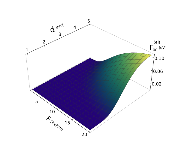
Figure 1: The width $\Gamma_{00}^{(\mbox{\tiny{el}})}$ of the ground exciton peak versus the ribbon width $d$ and electric field strength $F$. The width $\Gamma_{00}^{(\mbox{\tiny{el}})}$, quantum number $\kappa_{00}$ and factor $\Omega_{00}$ are determined via eqs. (34), (29) and (27), respectively, for the ribbon placed on the sapphire substrate $q=0.24$.

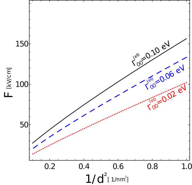
Figure 2: The isowidths curves $\Gamma_{00}^{(\mbox{\tiny{el}})}(d,F)=\mbox{const.}$ for the ground exciton peak. The width $\Gamma_{00}^{(\mbox{\tiny{el}})}$, quantum number $\kappa_{00}$ and factor $\Omega_{00}$ are determined from the same equations and for the same ribbon substrate as those used in Fig.1. The values of $\Gamma_{00}^{(\mbox{\tiny{el}})}$ are chosen to be $0.10;~{}0.06;~{}0.02~{}(\mbox{meV})$.

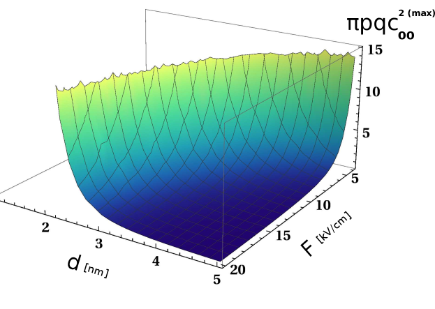
Figure 3: The dependence of the ground exciton peak maximum $c_{00}^{2\mbox{\tiny(max)}}$ on the ribbon width $d$ and electric field strength $F$. The coefficient $c_{00}^{2\mbox{\tiny(max)}}$, quantum number $\kappa_{00}$ and factor $\Omega_{00}$ are determined from the same equations and for the same substrate as in Fig.1.

Eq. (34) shows that within the $N$ Rydberg series the lowest absorption line considerably surpasses the excited peaks in narrowness $\Gamma_{N0}^{\left(\mbox{\tiny{el}}\right)}<<\Gamma_{Nn}^{\left(\mbox{\tiny{el}}\right)}$ and intensity $\alpha_{N0}^{\mbox{\tiny(max)}}>>\alpha_{Nn}^{\mbox{\tiny(max)}},~{}n=1,2,\ldots$. Fig. 3 demonstrates the dependence of the ground exciton peak maximum $c_{00}^{2(\mbox{\tiny{max}})}$ on the ribbon width $d$ and electric field strength $F$.

Eq. (27) allows us to introduce the parameter of the exciton state relative stability $Q_{Nn}$ in the ribbon with width $d$ exposed to the electric field $F$. This parameter generated by the condition $f_{N}\kappa_{Nn}^{3}=1$ becomes

$$Q_{Nn}(q)=\frac{\pi^{2}p}{8e}\mid N-\tilde{\sigma}\mid^{2}\frac{q^{3}}{\kappa_{Nn}^{3}};\quad\frac{\pi^{2}p}{8e}=0.82~{}\mbox{Vnm}$$ (57)

where $\kappa_{Nn}(q)$ is the root of eq. (29). Under the condiiton $Fd^{2}>Q_{Nn}(q)$ the $Nn$ state is practically ionized, while in the opposite case $Fd^{2}<Q_{Nn}(q)$ the state in question remains relatively stable. An electric field providing the relatively small width of the ground peak $\kappa_{N0}<1$ would be sufficiently strong to ionize completely the excited states $\kappa_{Nn}>n,\,n=1,2,\ldots$. Note that the parameter $Q_{Nn}(q)$ possesses a universal character as far as it depends only on the dimensionless exciton potential strength $q$.

5.1.2 Franz-Keldysh exciton absorption $\hbar\omega<\Delta_{N}$

As pointed out originally by Merkulov and Perel [18] the mechanism of the interband electroabsorption in bulk materials in the spectral regions distant from the exciton maxima is the F-K effect [16] (i.e. optical transition assisted by the interband carriers tunneling) strongly modified by the exciton attraction. This is completely in line with eqs. (35)-(37) relevant to the exciton electroabsorption and F-K effect in the AGNR. In the latter this spectrum depends both on the electric fields $F$ and ribbon width $d$, while in the semiconductor structures, i.e. in bulk crystals as well as in those subject to strong magnetic fields [40] and QWR [11] mostly only electric fields $F$ influence the optical absorption spectrum. It follows from eqs. (35)-(37) in which

$$\frac{1}{f_{N}\kappa_{N}^{3}}=(\Delta_{N}-\hbar\omega)^{\frac{3}{2}}\left(\frac{\mid N-\tilde{\sigma}\mid\pi}{8e^{2}pF^{2}d}\right)^{\frac{1}{2}}$$

that the stronger the electric field $F$ or/and ribbon width $d$ is, the larger are the exciton electroabsorption $c_{N}^{2}$ (35), F-K absorption $c_{N\tiny{(F-K)}}^{2}$ (36) and the smaller is the exciton attraction influence $T_{N}$ (37). Note that along with this the exciton peak maxima decrease. The exciton effect increases for frequencies close the exciton peaks for which $Y_{N}\ll 1$ and then decreases for intermediate frequencies corresponding to the regions $0<\kappa_{N}<\beta_{N0},\,n+\beta_{Nn}<\kappa_{N}<n+1,\sim n=0,1,2,\ldots.$ However, even for these frequencies the exciton effect contributes significantly to the optical absorption. As the frequency shifts away from the ground exciton peak $N=n=0$ inside the gap $(\kappa_{N}\rightarrow 0)$ the exciton effect becomes negligibly small, $\Gamma^{2}(-\kappa_{N})\simeq 4Y_{N}^{2}~{}\mbox{and}~{}c_{N}^{2}\simeq c^{2}_{N\mbox{\tiny(F-K)}}$. The spectrum of the exciton and F-K electroabsorption in the vicinity of the ground exciton peak and below and above in the intermediate frequency regions is given in Fig. 4. In this Figure one can see that in accordance with eqs. (35) and (37) in the vicinity of the ground exciton peak the exciton electroabsorbtion contributes considerably, while the F-K absorption (36) is nearly invisible. As mentioned above the chosen electric field corresponds to a relatively narrow ground peak and practically unites the first excited broad peak with the region of the continuous spectrum $\hbar\omega>\Delta_{N}.$

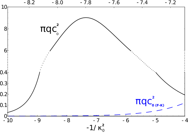
Figure 4: The spectra of the exciton electroabsorption in the vicinity of the ground exciton peak (black line) and of F-K absorption (blue line) as a function of the reciprocal frequency shift $-\kappa_{0}^{-2}=Ry_{0}/(\hbar\omega-\Delta_{0})$ with respect to the ground threshold $\Delta_{0}$. The coefficients $c_{0}^{2}~{}\mbox{and}~{}c_{0(\mbox{\tiny{F-K}})}^{2}$, functions $Y_{0}~{}\mbox{and}~{}\Omega_{0}$ are calculated from eqs. (28) and (36), (26) and (27), respectively, for $N=0$. The dimensionless electric field is chosen to be $f_{0}=5$; sapphire substrate $q=0.24$ is implied.

5.2 Franz-Keldysh exciton absorption $\hbar\omega>\Delta_{N}$

In the frequency region above the edge of the electroabsorption spectrum is described by eqs. (44). The frequency oscillations modulated by the reciprocal square-root factor (1D F-K effect [41]) are modified by the 1D exciton Sommerfeld factor $Z$ and the exciton phase shift $\Delta\Theta_{NZ}$. In contrast to semiconductor structures, in particular the bulk crystals subject to strong magnetic field $B$ [41] and QWR [11] in which the oscillation period depends only on the electric fields $F$, in the AGNR this period is affected by both the electric fields $F$ and ribbon width $d$. With increasing each of these parameters the oscillation period increases, while the phase shift $\Delta\Theta_{NZ}$ decreases. The Sommerfeld factor demonstrates that the exciton attraction suppresses the low energy oscillations and has only a small effect on those of high frequencies positioned away from the edge $\Delta_{N}$.

It is reasonable to compare the exciton absorption dependencies on the electric field $F$ and ribbon width $d$ with those of the quasi-1D semiconductor structures i.e. with the DE [40] and QWR [11]. The confinement radius $r_{0}$ analogical to the ribbon width $d$ is the magnetic length $a_{B}=\left(\frac{\hbar}{eB}\right)~{}\mbox{or wire radius}~{}R$, respectively. This radius was assumed to be much smaller than the semiconductor exciton Bohr radius $a=\frac{4\pi\varepsilon_{0}\varepsilon\hbar^{2}}{\mu e^{2}}$. The dependencies of the absorption spectrum on the electric fields $F$ are common for the AGNR and semiconductor structures. The weak electric field does not affect the peak positions and exciton binding energies, while it modifies considerably the shape of the spectrum. With increasing electric field the exciton peaks become broader and lower in intensity (eq. (34) ), absorption grow in the interpeak regions (eq. (35)) and frequency oscillations above the edge (eq. (44)) become rare. In contrast to the electric field effect the influence of the ribbon width $d$ is more pronounced compared to that of the wire radius $R$ or magnetic field $B$.

The exciton binding energies $E_{Nn}^{\mbox{\tiny(b)}}$ in the AGNR increase linearly with narrowing the ribbon $E_{Nn}^{\mbox{\tiny(b)}}\sim\Delta_{N}\sim d^{-1}$, while in the semiconductor structures this dependence has the less pronounced logarithmic character $E_{N0}^{\mbox{\tiny(b)}}\sim\ln^{2}\frac{r_{0}}{a}$ for the ground state $n=0$ and is practically invisible for the excited states $n=1,2,\ldots$. In the AGNR the confinement dependence of the exciton peak widths (eq. (34) ) are mostly governed by the exponential factor $\Gamma_{Nn}\sim d^{-1}\exp\left(-\frac{\mbox{const.}}{Fd^{2}}\right)$. This results in a peak widths decrease with the ribbon narrowing. In the semiconductor structures the ground peak $n=0$ becomes wider with decreasing radius $r_{0}~{}\Gamma_{N0}\sim\ln^{2}\frac{r_{0}}{a}$, while the excited peak widths $\Gamma_{Nn},~{}n=1,2,\ldots$ remain constant. In the AGNR the absorption maxima (34) $\alpha_{Nn}^{\mbox{\tiny(max)}}\sim\exp\left(\frac{\mbox{const.}}{Fd^{2}}\right)$. In semiconductor structures the confinement provides only the power growth modified by the logarithmic factor $\alpha_{Nn}^{\mbox{\tiny(max)}}\sim\left(r_{0}\ln\frac{r_{0}}{a}\right)^{-2},\,n\neq 0,\alpha_{N0}^{\mbox{\tiny(max)}}\sim r_{0}^{-2}\mid\ln\frac{r_{0}}{a}\mid^{-1}$. However, there is an exception from the above regarding the similar dependence of the peak positions. With increasing the confinement (decreasing the radius $r_{0}$ and width $d$) the exciton peaks shift towards higher frequencies in all structures.

In the frequency region below the edge $\hbar\omega<\Delta_{N}$ the F-K optical absorption in the AGNR (36) and the effect of the exciton attraction (37) depend on the parameters $F~{}\mbox{and}~{}d$ exponentially and by power law, respectively. In the semiconductor structures the coefficient of the F-K absorption demonstrates the less pronounced power dependence $\alpha_{\mbox{(\tiny F-K)}}\sim r_{0}^{-2}$, while the effect of the electron-hole attraction does not depend on the confinement. In the spectral region above the edge $\hbar\omega>\Delta_{N}$ the oscillations of the F-K absorption (44) become large in period with widening the AGNR, while in the semiconductor structures the confinement does not modify the oscillation period.

5.3 The double subband approximation

Note that all exciton states related to the excited Rydberg series $N\geq 1$ are initially meta-stable. This stems from their coupling to the states of the continuous spectra emanating from the energetically low-lying thresholds $\Delta_{N-1}$. At $F=0$ the latter causes the autoionization and transforms the $N\neq 0$ series of the strictly discrete states into the quasi-discrete ones (Fano resonances) with the energy widths $\Gamma_{Nn}^{(\mbox{\tiny{F}})}\sim\Delta_{N}\sim d^{-1}$ (eq.(54)), which increase with decreasing the ribbon width $d$ [33]. The optical absorption coefficient caused by the transitions to these exciton resonant states has been calculated in Ref. [12]. In the presence of an electric field $F$ the electroionization superimposes on the autoionization that in turn leads to the summation of the width $\Gamma_{Nn}^{(\mbox{\tiny{el}})}~{}\mbox{and}~{}\Gamma_{Nn}^{(\mbox{\tiny{F}})}$ determined by eqs. (34) and (54), respectively. However, the contribution of each of those widths to the total width $\Gamma_{Nn}^{(\mbox{t})}=\Gamma_{Nn}^{(\mbox{\tiny{el}})}+\Gamma_{Nn}^{(\mbox{\tiny{F}})}$ is different for the wide and narrow ribbons. The reason for this is that the widths $\Gamma_{Nn}^{(\mbox{\tiny{el}})}~{}\mbox{and}~{}\Gamma_{Nn}^{(\mbox{\tiny{F}})}$ change with varying ribbon width $d$ in the opposite way. The larger $d$ the less is the Fano width $\Gamma_{Nn}^{(\mbox{\tiny{F}})}$ and the width $\Gamma_{Nn}^{(\mbox{\tiny{el}})}$ becomes larger. Thus, for the narrow AGNR the Fano coupling surpasses the electric field tunneling and $\Gamma_{Nn}^{(\mbox{\tiny{F}})}>\Gamma_{Nn}^{(\mbox{\tiny{el}})}$. With further ribbon widening both effects become equal and then the electric field ionization dominates that of autoionization. For stronger electric field $F$ the critical ribbon width $d_{F}$ decreases providing the peak widths equality $\Gamma_{Nn}^{(\mbox{\tiny{F}})}=\Gamma_{Nn}^{(\mbox{\tiny{el}})}$. As it follows from eqs. (34) and (54) the latter condition implies the relationship $d^{2}F\simeq\mbox{const.}$ The exciton peak widths $\Gamma_{Nn}^{(\mbox{\tiny{F}})}~{}\mbox{and}~{}\Gamma_{Nn}^{(\mbox{\tiny{el}})}$ as a function of the ribbon width $d$ for the different electric field strengths $F$ are presented in Fig.5. Note that our results for the ground $n=0$ exciton state related to the ground Rydberg series $N=0$ are qualitatively valid for any states and any series.

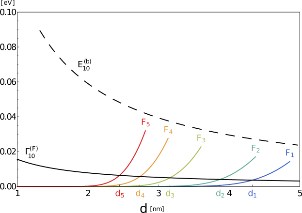
Figure 5: The ground $n=0$ exciton peak widths $\Gamma_{10}^{(\mbox{\tiny{el}})}$ (34) corresponding to different electric fields $F_{1}=8,F_{2}=10,F_{3}=15,F_{4}=20,F_{5}=25$ in units kV/cm (color lines), $\Gamma_{10}^{(\mbox{\tiny{F}})}$ (54) induced by intersubband coupling (black line) and the binding energy $E_{10}^{\mbox{\tiny(b)}}=\mid W_{10}\mid$ (33) (dashed line) versus the ribbon width $d$. The first excited Rydberg series $N=1$ is addressed. The ribbon is placed on the sapphire substrate $q=0.24$

.

In an effort to connect our results closer to experiment, we estimate the expected values for the AGNR with width 4 nm of the family specified by $\tilde{\sigma}=\frac{1}{3}$ and placed on the sapphire substrate $q=0.24$. The peak positions $\hbar\omega=E_{Nn}$, binding energies $E_{Nn}^{\mbox{\tiny(b)}}$, widths $\Gamma_{Nn}^{(\mbox{\tiny{el}})}$, peak absorption maxima $c_{Nn}^{2\mbox{\tiny(max)}}$, exciton $c_{N}^{2}$ and F-K electroabsorption $c_{N\mbox{\tiny(F-K)}}^{2}$ coefficients are presented for the ground $n=0$ and first excited $n=1$ peaks related to the ground subband $N=0$. Using the quantum numbers $\kappa_{0n}$ from eq. (29) we obtain $E_{00}=316.1~{}\mbox{meV}$, $E_{01}=338.7~{}\mbox{meV}$ and $E_{00}^{\tiny\mbox{(b)}}=23.9~{}\mbox{meV}$, $E_{01}^{\mbox{\tiny(b)}}=1.38~{}\mbox{meV}$ for the peak positions and binding energies, respectively. Since the ground state binding energy significantly exceeds that of the first excited state the critical electric field $\bar{F}_{00}\simeq 24~{}\frac{\mbox{\tiny{kV}}}{\mbox{\tiny{cm}}}$ is much larger than $\bar{F}_{01}\simeq 0.31~{}\frac{\mbox{\tiny{kV}}}{\mbox{\tiny{cm}}}$. These fields satisfying the condition $\bar{F}_{Nn}=Q_{Nn}d^{-2}$ (eq. (57)) are the upper bounds of the fields, providing the complete depletion of the bound exciton state and the disappearance of the peak from the optical spectrum. Note that the critical fields providing the equality of the binding energies $E_{Nn}^{\mbox{\tiny(b)}}$ and spectral widths $\Gamma_{Nn}^{(\mbox{\tiny{el}})}$ can be smaller by a significant factor than those presented above. In the presence of an electric field $F=7~{}\frac{\mbox{\tiny{kV}}}{\mbox{\tiny{cm}}}$ the ground peak width becomes $\Gamma_{Nn}^{(\mbox{\tiny{el}})}=7.56~{}\mbox{meV}$ yielding for the lifetime $\tau=\hbar/\Gamma_{00}=0.082~{}\mbox{ps}$. This allows us to conclude that for weak electric fields of the order of $F\leq 10~{}\frac{\mbox{\tiny{kV}}}{\mbox{\tiny{cm}}}$ the ground exciton peaks $N\scriptsize{\text{0}}$ remain relatively narrow and accessible to an experimental study, while for strong fields of several tens of kV/cm provide a complete ionization of the exciton states and liberation of the carriers in the AGNR with widths of several nanometers.

In the spectral region below the edge $\hbar\omega<\Delta_{0}$ the electron-hole attraction considerably enhances the absorption for the frequencies positioned far away from the exciton peaks. It follows from eq. (37) that in the presence of an electric field $F=7~{}\frac{\mbox{\tiny{kV}}}{\mbox{\tiny{cm}}}$ the exciton electroabsorption deeply penetrating into the gap $(\Delta_{0}-\hbar\omega\simeq 3.2E_{00}^{\mbox{\tiny(b)}}\simeq 30Ry_{0})$ exceeds that of the F-K by a factor of $T_{0}\simeq 8.6$. In contrast to the discrete part of the spectrum, for frequencies positioned above the edge $\hbar\omega>\Delta_{0}$ the exciton effect significantly reduces the magnitude of the F-K oscillations which is reflected in the Sommerfeld factor $Z_{0}$ in eq. (44). It follows from this equation that in the frequency region $\hbar\omega-\Delta_{0}\simeq 4Ry_{0}$ and for the electric field $F=7~{}\frac{\mbox{\tiny{kV}}}{\mbox{\tiny{cm}}}$ the reduction of the oscillating magnitudes is given by $Z_{0}=0.30$. The corresponding phase is $\Delta\Theta_{0Z}=-0.44\pi$.

Intending to compare our analytical results with those calculated numerically we refer to Ref. [42] in which the analogous quasi-1D structure, namely the QWR with radius $R$ subject to an electric field polarized along the wire axis has been studied. The theoretical approach relied upon the Dirac equation relevant to the electron (hole) dispersion law $E(k)=\pm\hbar v_{F}\sqrt{(2R)^{-2}+k^{2}}$ ($k$ is the longitudinal electron (hole) momentum) similar to that for an AGNR [31]. The following results for the exciton electroabsorbtion have been reported. Narrow wires $(R)$ show larger exciton binding energies $E^{(\tiny{b})}$. Electric fields $(F)$ enhance the subgap $(\hbar\omega<\Delta)$ optical absorption. The electric fields $(F)$ induce the F-K oscillations. Influence of a given electric field $(F)$ on the excitonic absorption peak decreases as the Coulomb interactions $(q)$ are made stronger. Clearly, these conclusions are qualitatively in complete line with ours (see eqs. (33) for $E_{Nn}^{(\tiny{b})}=-W_{Nn}$, (36) and Fig.4 for $c_{N\tiny{(F-K)}}^{2}$, (44) for F-K oscillations and (27) for $\Omega_{N}$ and $f_{N}=F/F_{N}$ with $F_{N}\sim q^{3}$, respectively.) The differences in AGNR and QWR topologies in our paper and in Ref. [42], respectively prevents a detailed quantitative comparison.

As well known, the $\mbox{SiO}_{2}$ substrate $\varepsilon=3.9$ is widely used in experiments. Nevertheless, we were forced to refrain from the estimates of the possible experimental data related to this material. The problem is here that the corresponding adiabatic parameter $q=0.37$ is not sufficiently small to provide the needed accuracy implying $q\ll 1$. In principle, the case of similar parameter values can be investigated by solving the basic set of eqs. (11) numerically. Also, we avoid too narrow ribbons with width of 1-2 nm, consisting of several 1D unit cell distances, to be taken as a candidates for the above-mentioned estimates. In these ribbons its discrete structure manifests itself and the continual approach based on the Dirac equation becomes inappropriate.

The presented analytical results and numerical estimates show that in the AGNR with typical widths and subject to laboratory electric fields the exciton effect manifests itself in the optical absorption spectrum. An electron-hole attraction on the one hand side significantly modifies the absorption for a very wide frequency region below and above the absorption edge and on the other hand side demonstrates that the exciton peaks are sufficiently narrow and accessible to experimental study. We believe that our developed analytical approach highlights the mechanism of the exciton electroabsorption in AGNR and the auto- and electroionization processes favoring the deliberation of carriers. Also we hope that estimates of the expected experimental values could be usful in further studies of graphene nanoribbons and their applications in opto- and microelectronics.

6 Conclusion

In summary, we have developed an analytical approach to the problem of the exciton absorption in a narrow armchair graphene nanoribbon (AGNR) exposed to an external electric field directed parallel to the graphene axis. The effect of the strong ribbon confinement was assumed to be much stronger than that of the exciton Coulomb electric field, which in turn considerably exceeds the external field. In the approximation of the isolated size-quantized subbands the exciton absorption coefficient of light polarized parallel to the ribbon axis has been determined in an explicit form. We traced the dependencies of the exciton peak positions, their widths caused by the electric fields and intensities of the continuous absorption bands on the ribbon width and electric field strength. With increasing electric field and widening the ribbon the exciton peak increases in width and decreases in intensity maximum. The exciton electron-hole attraction strongly modifies the Franz-Keldysh (F-K) absorption related to the unbound carriers significantly increasing and reducing the F-K absorption in the interpeak regions below and above the edge, respectively. In the double subband approximation the double channel ionization of the exciton discrete states adjacent to the first excited size-quantized energy level has been considered. These channels are open due to the tunneling caused by the electric field and autoionization induced by the Fano coupling of these states to the states of the continuous spectrum of the ground subband. The total exciton peak widths caused by the electro- and autoionization have been determined. The presented analytical results correlate well with those previously calculated numerically.

Estimates of the expected experimental values for realistic AGNR and electric fields yield two aspects of the electric field effect. Weak electric fields provide a significantly long exciton lifetime and excitons remain available for an optical study and use in optoelectronics. A relatively strong field ionizing the excitons make the carriers unbound and promote the AGNR transport properties.

7 Acknowledgments

The authors are grateful to A. Devdariany for useful discussion and M. Pyzh for significant technical assistance.

References

- [1] M. Fujita, K. Wakabayashi, K. Nakada, and K. Kusakabe, J. Phys. Soc. Jpn. 65, 1920 (1996)
- [2] K. Wakabayashi, K. Sasaki, T. Nakanishi, Sci. Technol. Adv. Mater. 11, 054504 (2010)
- [3] J. Alfonsi and M. Meneghetti, New J. Phys. 14, 053047 (2012)
- [4] G. Soavi, S. D. Conte, C. Manzoni, D. Viola, A. Narita, Y. Hu, X. Feng, U. Hohenester, E. Molinari, D. Prezzi, K. Müllen and G. Cerullo, Nat. Commun. 7, 11010 (2016)
- [5] Y. L. Jia, X. Geng, H. Sun and Y. Luo, Eur. Phys. J. B 83, 451 (2011)
- [6] A. H. Castro Neto, F. Guinea, N. M. R. Peres, K. S. Novoselov, and A. K. Geim, Rev. Mod. Phys. 81, 109 (2009)
- [7] L. Yang, M. Cohen and S. Louie, Nano Lett. 7, 3112 (2007)
- [8] T. Y. Zhang and W. Zhao, Phys. Rev. B 73, 245337 (2006)
- [9] J. R. Madureira, M. Z. Maialle, and M. H. Degani, Phys. Rev. B 66, 075332 (2002)
- [10] A. G. Zhilich and O. A. Maksimov, Sov. Phys. Semicond. 15, 1108 (1981)
- [11] B. S. Monozon and P. Schmelcher, Phys. Rev. B 79, 165314 (2009)
- [12] B. S. Monozon and P. Schmelcher, Physica B 500,89 (2016)
- [13] U. Fano, Phys. Rev. B 124, 1866 (1961)
- [14] H. Hasegawa and R.E. Howard, J. Phys. Chem. Solids 21, 179 (1961)
- [15] D. S. Novikov, Phys. Rev. B 76, 245435 (2007)
- [16] W. Franz, Z. Naturforsch. A 13, 484 (1958); L. V. Keldysh, Sov. Phys. JETP 34, 788 (1958)
- [17] Theory of Excitons, (Academic Press, New York and London, 1963)
- [18] I. A. Merkulov and V. I. Perel’, Phys. Lett. 45, 83 (1973)
- [19] A. G. Aronov and A. S. Iosilevich, Sov. Phys. JETP 47, 548 (1978)
- [20] T. Yamabe, A. Tachibana and H. J. Silverstone, Phys. Rev. A 16, 877 (1977)
- [21] D. Prezzi, D. Varsano, A. Ruini, A. Marini and E. Molinari, Phys. Rev. B 77, 041404(R) (2008)
- [22] X. Zhu and H. Su, J. Phys. Chem. A 115, 11998 (2011)
- [23] R. Denk, M. Hohage, P. Zeppenfeld, J. Cai, C. A. Pignedoli, H. Sode, R. Fasel, X. Feng, K. Mullen, S. Wang, D. Prezzi, A. Ferretti, A. Ruini, E. Molinari and P. Ruffieux Nature Communications 5, 4253 (2014)
- [24] Y. Lu, S. Zhao, W. Lu, H. Liu and W. Liang, J. Appl. Phys. 115, 103701 (2014)
- [25] K. Gundra and A. Shukla, Phys. Rev. B 83, 075413 (2011)
- [26] L. Mohammadzadeh, A. Asgari, S. Shojaei and E. Ahmadi, Eur. Phys. J. B 84, 249 (2011)
- [27] Ken-ichi Sasaki, K. Kato, Y. Tokura, K. Oguri and T. Sogawa, Phys. Rev. B 84, 085458 (2011)
- [28] R. J. Elliot, Phys. Rev. B 108, 1384 (1957)
- [29] B. S. Monozon and P Schmelcher, Phys. Rev. B 71, 085302 (2005)
- [30] M. M. Mahmoodian and M. V. Entin, Nanoscale Res. Lett. 7, 599 (2012)
- [31] L. Brey and H. A. Fertig, Phys. Rev. B 73, 235411 (2006)
- [32] E. H. Hwang and S.Das Sarma, Phys. Rev. B 75, 205418 (2007)
- [33] B. S. Monozon and P Schmelcher, Phys. Rev. B 86, 245404 (2012)
- [34] B. S. Monozon and P Schmelcher, Phys. Rev. B 90, 125313 (2014)
- [35] Handbook of Mathematical Functions, edited by M. Abramowitz and I. A. Stegun (Dover, New York, 1972)
- [36] S. Yu. Slavyanov, Asymptotic Solution to the One-dimensional Schrödinger Equation (American Mathematical Society, Philadelphia, PA, 1996)
- [37] R. G. Newton, Scattering Theory of Waves and Particles(Springer, New York, 1982)
- [38] P. V. Ratnikov and A. P. Silin, JETP 114, 512 (2012)
- [39] A. Dalgarno and J. T. Lewis, Proc. R. Soc. London A 233, 70 (1955)
- [40] B. S. Monozon, Sov. Phys. Solid State 18, 275 (1976)
- [41] C. Ciobanu, Rev. Roumaine Phys. 10, 109 (1965)
- [42] I. Garate and M. Franz, Phys. Rev. B 84, 045403 (2011)