Double, borderline, and extraordinary eigenvalues of Kac–Murdock–Szegő matrices
with a complex parameter

Abstract.

For all sufficiently large complex $\rho$, and for arbitrary matrix dimension $n$, it is shown that the Kac–-Murdock–-Szegő matrix $K_{n}(\rho)=\left[\rho^{|j-k|}\right]_{j,k=1}^{n}$ possesses exactly two eigenvalues whose magnitude is larger than $n$. We discuss a number of properties of the two “extraordinary” eigenvalues. Conditions are developed that, given $n$, allow us—without actually computing eigenvalues—to find all values $\rho$ that give rise to eigenvalues of magnitude $n$, termed “borderline” eigenvalues. The aforementioned values of $\rho$ form two closed curves in the complex-$\rho$ plane. We describe these curves, which are $n$-dependent, in detail. An interesting borderline case arises when an eigenvalue of $K_{n}(\rho)$ equals $-n$: apart from certain exceptional cases, this occurs if and only if the eigenvalue is a double one; and if and only if the point $\rho$ is a cusp-like singularity of one of the two closed curves.

1. Introduction

This paper is a direct continuation of [1]. For $\rho\in\mathbb{C}$, it deals with the complex-symmetric Toeplitz matrix

(1.1) $$K_{n}(\rho)=\left[\rho^{|j-k|}\right]_{j,k=1}^{n}=\begin{bmatrix}1&\rho&\rho^{2}&\ldots&\rho^{n-1}\\ \rho&1&\rho&\ldots&\rho^{n-2}\\ \rho^{2}&\rho&1&\ldots&\rho^{n-3}\\ \vdots&\vdots&\vdots&\ddots&\vdots\\ \rho^{n-1}&\rho^{n-2}&\rho^{n-3}&\ldots&1\end{bmatrix}.$$

For the special case $0<\rho<1$, $K_{n}(\rho)$ is often called the Kac–-Murdock–-Szegő matrix; see [1] for a history and a discussion of applications. Assuming throughout that $n=2,3,\ldots$, we categorize the eigenvalues of $K_{n}(\rho)$ as follows.

Definition 1.1.

Let $\rho\in\mathbb{C}$. An eigenvalue $\lambda\in\mathbb{C}$ of $K_{n}(\rho)$ is called ordinary if $|\lambda|\leq n$ and extraordinary if $|\lambda|>n$.

The terms ordinary/extraordinary are consistent with Section 6 of [1], the investigation of which pertains only to the special case $\rho\in\mathbb{R}$ (this is when $K_{n}(\rho)$ is a real-symmetric matrix). Ref. [1] further discusses a number of connections between extraordinary eigenvalues and the notions of wild, outlying, and un-Szegő-like eigenvalues developed by Trench [2], [3], [4].

Definition 1.2.

Let $\rho\in\mathbb{C}$. An eigenvalue $\lambda\in\mathbb{C}$ of $K_{n}(\rho)$ is called borderline if $|\lambda|=n$ and borderline/double if $\lambda$ is a borderline eigenvalue and, concurrently, an (algebraically) double eigenvalue.

Our main goal herein is to find the $\rho$ that give rise to borderline and extraordinary eigenvalues (the said values of $\rho$ are, of course, $n$-dependent). In other words, this paper extends the concept of extraordinary eigenvalues from the case $\rho\in\mathbb{R}$ to the case $\rho\in\mathbb{C}$, and develops conditions for the occurrence of extraordinary eigenvalues.

By Theorems 3.7 and 4.1 of [1] the eigenvalues of $K_{n}(\rho)$ ($\rho\in\mathbb{C}$) are either of type-1 or type-2. The two types are mutually exclusive. The most notable distinguishing feature is that type-1 (type-2) eigenvalues correspond to skew-symmetric (symmetric) eigenvectors, see Remark 4.3 of [1].

In the special case $\rho\in\mathbb{R}$, there are at most two extraordinary eigenvalues—one of each type—irrespective of how large $n$ is. In fact, using the notation

(1.2) $$\xi_{n}=\frac{n+1}{n-1},$$

it readily follows from the results in Section 6 of [1] and from Lemma 2.5 of [1] (that lemma is repeated as Lemma 2.1 below) that the following holds.

Proposition 1.3.

[1] Let $\rho\in\mathbb{R}$. The matrix $K_{n}(\rho)$ possesses an eigenvalue $\lambda$ that is borderline iff $\rho\in\{-\xi_{n},-1,1,\xi_{n}\}$. The specific value and type is as follows,

(i) $\rho=\xi_{n}$: $\lambda=-n$ is a type-1 borderline eigenvalue.

(ii) $\rho=1$: $\lambda=n$ is a type-2 borderline eigenvalue.

(iii) $\rho=-1$: $\lambda=n$ is a borderline eigenvalue that is of type-1 if $n=2,4,\ldots$ and of type-2 if $n=3,5,\ldots$.

(iv) $\rho=-\xi_{n}$: $\lambda=-n$ is a borderline eigenvalue that is of type-2 if $n=2,4,\ldots$ and of type-1 if $n=3,5,\ldots$.

Depending on the (real) value of $\rho$, Table 1 gives the number of type-1 extraordinary eigenvalues and the number of type-2 extraordinary eigenvalues.

value of $\rho$	number of type-1 extraordinary eigenvalues	number of type-2 extraordinary eigenvalues
$\rho<-\xi_{n}$	$1$	$1$
$-\xi_{n}\leq\rho<-1$	$\begin{cases}1,{\rm\,if\,\,}n=2,4,6,\ldots\\ 0,{\rm\,if\,\,}n=3,5,7,\ldots\end{cases}$	$\begin{cases}0,{\rm\,if\,\,}n=2,4,6,\ldots\\ 1,{\rm\,if\,\,}n=3,5,7,\ldots\end{cases}$
$-1\leq\rho\leq 1$	$0$	$0$
$1<\rho\leq\xi_{n}$	$0$	$1$
$\rho>\xi_{n}$	$1$	$1$

Table 1. Numbers (0 or 1) of extraordinary type-1 and extraordinary type-2 eigenvalues for the special case $\rho\in\mathbb{R}$.

The present paper will help us view Proposition 1.3 as a corollary of more general results for which $\rho\in\mathbb{C}$. And—as is often the case—the extension into the complex domain will help us better understand and visualize the special case $\rho\in\mathbb{R}$, including certain particularities of this case. Our figures, for example, will clearly illustrate that borderline/double eigenvalues can appear when $\rho\in\mathbb{C}\setminus\mathbb{R}$, but not when $\rho\in\mathbb{R}$.

2. Preliminaries

What follows builds upon results (or corollaries of results) from [1], given in this section as lemmas. Our first lemma is Lemma 2.5 of [1] (throughout this paper, the overbar denotes the complex conjugate).

Lemma 2.1.

[1] Let $\rho\in\mathbb{C}$, let $(\lambda,\mathbf{y})$ be an eigenpair of $K_{n}(\rho)$, and let $J_{n}$ be the signature matrix

$$J_{n}=\begin{bmatrix}1&0&\cdots&0&0\\ 0&-1&\cdots&0&0\\ \vdots&\vdots&\ddots&0&0\\ 0&0&\cdots&(-1)^{n-2}&0\\ 0&0&\cdots&0&(-1)^{n-1}\end{bmatrix}.$$

Then $K_{n}(\bar{\rho})$ and $K_{n}(-\rho)$ possess the eigenpairs $(\bar{\lambda},\bar{\mathbf{y}})$ and $(\lambda,J_{n}\mathbf{y})$, respectively.

If $\mathbf{y}$ is a symmetric (or skew-symmetric) vector, then $J_{n}\mathbf{y}$ remains symmetric (or skew-symmetric) if $n$ is odd, but becomes skew-symmetric (or symmetric) if $n$ is even. Lemma 2.1 thus gives the following result.

Lemma 2.2.

For $\rho\in\mathbb{C}$, let $\lambda$ be a type-1 (or type-2) eigenvalue of $K_{n}(\rho)$. Then
(i) $\bar{\lambda}$ is a type-1 (or type-2) eigenvalue of $K_{n}(\bar{\rho})$.
(ii) For $n=3,5,7,\ldots$, $\lambda$ is a type-1 (or type-2) eigenvalue of $K_{n}(-\rho)$.
(iii) For $n=2,4,6,\ldots$, $\lambda$ is a type-2 (or type-1) eigenvalue of $K_{n}(-\rho)$.

Theorems 4.1, 4.5, and 6.5 of [1] imply the lemma that follows.

Lemma 2.3.

[1] Let $\rho\in\mathbb{C}$. $\lambda\in\mathbb{C}$ is a type-1 (or type-2) eigenvalue of $K_{n}(\rho)$ iff

(2.1) $$\lambda=-\frac{\sin(n\mu)}{\sin{\mu}}\quad\left({\rm or}\,\,\lambda=\frac{\sin(n\mu)}{\sin{\mu}}\right),$$

where $\mu\in\mathbb{C}$ satisfies

(2.2) $$\rho=\frac{\sin{\frac{(n+1)\mu}{2}}}{\sin{\frac{(n-1)\mu}{2}}}\quad\left({\rm or}\,\,\rho=\frac{\cos{\frac{(n+1)\mu}{2}}}{\cos{\frac{(n-1)\mu}{2}}}\right).$$

For $\rho\in\mathbb{C}\setminus\{-1,0,1\}$, the $\lambda$ given by (2.1) is a repeated type-1 (or repeated type-2) eigenvalue iff, in addition to (2.2), $\mu$ satisfies

(2.3) $$\xi_{n}\cos{\frac{(n+1)\mu}{2}}=\rho\cos{\frac{(n-1)\mu}{2}}\quad\left({\rm or}\,\,\xi_{n}\sin{\frac{(n+1)\mu}{2}}=\rho\sin{\frac{(n-1)\mu}{2}}\right).$$

Proof.

Eqns. (2.1) and (2.2) follow from: (i) Theorem 4.1 of [1] when $\rho\neq\pm 1,\pm\xi_{n}$; (ii) Theorem 6.5 of [1] when $\rho=1$ or $\rho=\xi_{n}$; and (iii) Lemma 2.2 when $\rho=-1$ or $\rho=-\xi_{n}$ [use (ii) with $\mu+\pi$ in place of $\mu$]. The first equation in (2.3) (for the type-1 case) is (4.21) in Theorem 4.5 of [1], and the second one is entirely similar. ∎

Throughout, we also use the following elementary statements about the Chebyshev polynomial $U_{n-1}(t)$, where $t=\cos x$ or $t=\cosh x$.

Lemma 2.4.

For $n=2,3,4,\ldots$ and $x\in\mathbb{R}$, we have

(2.4) $$\left|\frac{\sin(nx)}{\sin x}\right|\leq n,$$

and

(2.5) $$\frac{\sinh(nx)}{\sinh x}\geq n.$$

Equality in (2.4) occurs iff $x=0,\pm\pi,\pm 2\pi,\ldots$. In (2.5), equality occurs iff $x=0$.

3. Double eigenvalues

Ref. [1] shows that (excluding certain trivial cases) the only repeated eigenvalues of $K_{n}(\rho)$ are double eigenvalues equal to $-n$. Theorem 3.1 recapitulates this and adds a converse result, namely that (barring exceptional cases) an eigenvalue equal to $-n$ is necessarily a double eigenvalue.

Theorem 3.1.

Let $\rho\in\mathbb{C}\setminus\{-\xi_{n},-1,0,1,\xi_{n}\}$ and let $\lambda$ be an eigenvalue of $K_{n}(\rho)$. Then the following three statements are equivalent:
(i) $\lambda$ is a repeated eigenvalue of $K_{n}(\rho)$.
(ii) $\lambda$ is a double eigenvalue of $K_{n}(\rho)$.
(iii) $\lambda=-n$.

Proof.

(ii) $\implies$ (i) is obvious, while (i) $\implies$ (ii) and (i) $\implies$ (iii) are in Theorem 4.5 of [1]. To show (iii) $\implies$ (i), let $-n$ be a type-1 (or type-2) eigenvalue of $K_{n}(\rho)$. Then, by Lemma 2.3,

(3.1) $$\frac{\sin(n\mu)}{\sin{\mu}}=n\quad\left({\rm or}\,\,\frac{\sin(n\mu)}{\sin{\mu}}=-n\right),$$

where $\mu$ satisfies (2.2). Eqns. (3.1) and (1.2) imply the equalities

$$\frac{\tan\frac{(n-1)\mu}{2}}{\tan\frac{(n+1)\mu}{2}}=\frac{1}{\xi_{n}}\quad\left({\rm or}\,\,\frac{\tan\frac{(n-1)\mu}{2}}{\tan\frac{(n+1)\mu}{2}}=\xi_{n}\right),$$

which, when combined with (2.2), yield (2.3). Therefore the eigenvalue $-n$ is a repeated one by Lemma 2.3, completing our proof. ∎

Remark 3.2.

In Theorem 3.1, all excluded values of $\rho$ are exceptional. The exceptions are as follows. When $\rho=\pm\xi_{n}$, $\lambda=-n$ is an eigenvalue (see Proposition 1.3) that is non-repeated by Proposition 6.1 of [1]. When $\rho=\pm 1$, $\lambda=0\neq-n$ is (at least when $n>2$) a repeated eigenvalue, see (2.7) of [1] or (6.22) of [1]. When $\rho=0$, finally, $\lambda=1\neq-n$ is a repeated eigenvalue of the identity matrix $K_{n}(0)$.

Corollary 3.3.

Let $\rho\in\mathbb{C}$. If $\lambda$ is a borderline/double eigenvalue of $K_{n}(\rho)$, then $\rho\in\mathbb{C}\setminus\mathbb{R}$ and $\lambda=-n$. By way of a converse, an eigenvalue $\lambda$ of $K_{n}(\rho)$ is a borderline/double eigenvalue if any one of the following statements is true:
(i) $\lambda$ is a double eigenvalue and $\lambda=-n$; or
(ii) $\lambda$ is a repeated borderline eigenvalue; or
(iii) $\lambda=-n$ and $\rho\neq\pm\xi_{n}$; or
(iv) $\lambda$ is a repeated eigenvalue, $\rho\neq\pm 1$, and $\rho\neq 0$.

Theorem 4.5 of [1] allows one to compute (via the solution to a polynomial equation) all $\rho\in\mathbb{C}$ for which $K_{n}(\rho)$ possesses a type-1 (or type-2) borderline/double eigenvalue.

4. Borderline eigenvalues and closed curves $B_{n}^{(1)}$, $B_{n}^{(2)}$

The theorem that follows is the heart of this paper, as it enables us to compute all complex values $\rho$ that give rise to type-1 (or type-2) borderline eigenvalues. The theorem specifically asserts that the said values of $\rho$ coincide with the range of a complex-valued function $f_{n}^{(1)}(u)$ [or $f_{n}^{(2)}(u)$], where $u\in[-\pi,\pi]$. The functions $f_{n}^{(1)}(u)$ and $f_{n}^{(2)}(u)$ are defined via the unique solution to a certain transcendental equation.

Theorem 4.1.

For $\rho\in\mathbb{C}$, $K_{n}(\rho)$ possesses a borderline type-1 eigenvalue $\lambda$ iff $\rho=f_{n}^{(1)}(u)$ and $\lambda=b_{n}^{(1)}(u)$ where

(4.1) $$f_{n}^{(1)}(u)=\frac{\displaystyle\sin{\frac{(n+1)\mu(n,u)}{2}}}{\displaystyle\sin{\frac{(n-1)\mu(n,u)}{2}}},\qquad b_{n}^{(1)}(u)=-\frac{\sin[n\mu(n,u)]}{\sin\mu(n,u)},$$

in which

(4.2) $$\mu(n,u)=u+iv(n,u).$$

In (4.2), $u\in[-\pi,\pi]$ is arbitrary while $v(n,u)$ is the function of $u$ that is defined as the unique non-negative root of the transcendental equation

(4.3) $$\sinh^{2}(nv)-n^{2}\sinh^{2}{v}=g_{n}(u),\quad v\geq 0,$$

in which

(4.4) $$g_{n}(u)=n^{2}\sin^{2}{u}-\sin^{2}(nu),\quad u\in[-\pi,\pi].$$

Similarly, $K_{n}(\rho)$ possesses a borderline type-2 eigenvalue $\lambda$ iff $\rho=f_{n}^{(2)}(u)$ and $\lambda=b_{n}^{(2)}(u)$ where

(4.5) $$f_{n}^{(2)}(u)=\frac{\cos{\displaystyle\frac{(n+1)\mu(n,u)}{2}}}{\cos{\displaystyle\frac{(n-1)\mu(n,u)}{2}}},\qquad b_{n}^{(2)}(u)=\frac{\sin[n\mu(n,u)]}{\sin\mu(n,u)},$$

in which, once again, $u\in[-\pi,\pi]$ is arbitrary and $\mu(n,u)$ is found from (4.2)–(4.4).

Proof.

In Lemma 2.3, take $|\lambda|=n$ and set $u={\rm Re}\mu$ and $v={\rm Im}\mu$ to see that $K_{n}(\rho)$ has a borderline type-1 eigenvalue $\lambda$ iff $\rho=\rho_{n}(u,v)$ and $\lambda=\lambda_{n}(u,v)$ where

(4.6) $$\rho_{n}(u,v)=\frac{\displaystyle\sin{\frac{(n+1)u}{2}}\cosh{\frac{(n+1)v}{2}}+i\cos{\frac{(n+1)u}{2}}\sinh{\frac{(n+1)v}{2}}}{\displaystyle\displaystyle\sin{\frac{(n-1)u}{2}}\cosh{\frac{(n-1)v}{2}}+i\cos{\frac{(n-1)u}{2}}\sinh{\frac{(n-1)v}{2}}},\quad u,v\in\mathbb{R},$$

and

(4.7) $$\lambda_{n}(u,v)=-\frac{\sin[n(u+iv)]}{\sin(u+iv)},\quad u,v\in\mathbb{R},$$

where $u$, $v$, and $n$ are interrelated via

(4.8) $$n^{2}=\frac{\sin^{2}(nu)+\sinh^{2}(nv)}{\sin^{2}{u}+\sinh^{2}{v}},\quad u,v\in\mathbb{R}.$$

Since the right-hand sides of (4.6)–(4.8) are $2\pi$-periodic in $u$, we assume $u\in[-\pi,\pi]$ with no loss of generality. Since, also, $\rho_{n}(-u,-v)=\rho_{n}(u,v)$ and $\lambda_{n}(-u,-v)=\lambda_{n}(u,v)$, we further assume $v\geq 0$.

Eqn. (4.8) is then equivalent to the definition (4.4) and the transcendental equation (4.3). This equation has a unique solution $v=v(n,u)\geq 0$ because: (i) $g_{n}(u)\geq 0$ for $u\in[-\pi,\pi]$; and (ii) the left-hand side of (4.3) vanishes when $v=0$ and has a positive derivative in $(0,+\infty)$ (assertions (i) and (ii) are readily shown via Lemma 2.4).

With $v=v(n,u)$ thus determined, the $\rho_{n}(u,v)$ of (4.6) and the $\lambda_{n}(u,v)$ of (4.7) are no longer functions of $v$, and the notations $f_{n}^{(1)}(u)=\rho_{n}(u,v)$ and $b_{n}^{(1)}(u)=\lambda_{n}(u,v)$ prove (4.1) with (4.2). We have thus shown all assertions pertaining to type-1 eigenvalues.

For the type-2 case, proceed as before with

$$\rho_{n}(u,v)=\frac{\displaystyle\cos{\frac{(n+1)u}{2}}\cosh{\frac{(n+1)v}{2}}-i\sin{\frac{(n+1)u}{2}}\sinh{\frac{(n+1)v}{2}}}{\displaystyle\displaystyle\cos{\frac{(n-1)u}{2}}\cosh{\frac{(n-1)v}{2}}-i\sin{\frac{(n-1)u}{2}}\sinh{\frac{(n-1)v}{2}}},\quad u,v\in\mathbb{R},$$

in place of (4.6), and with the opposite sign in (4.7). Otherwise, the proof is identical. ∎

The lemma that follows lists some properties (to be used several times throughout) of the functions of $u$ encountered in Theorem 4.1.

Lemma 4.2.

(i) The real and imaginary parts of the functions $f_{n}^{(1)}(u)$ and $f_{n}^{(2)}(u)$ can be found from

(4.9) $$f_{n}^{(1)}(u)=\frac{[\cos u\cosh(nv)-\cos(nu)\cosh v]-i[\sin u\sinh(nv)-\sin(nu)\sinh v]}{\cosh[(n-1)v]-\cos[(n-1)u]},$$

(4.10) $$f_{n}^{(2)}(u)=\frac{[\cos u\cosh(nv)+\cos(nu)\cosh v]-i[\sin u\sinh(nv)+\sin(nu)\sinh v]}{\cosh[(n-1)v]+\cos[(n-1)u]},$$

in which $v$ stands for the $v(n,u)$ of (4.3)–(4.4), for which

$$v(n,u)=v(n,-u)=v(n,\pi-u).$$

(ii) Let $k=1$ or $k=2$ and let $u\in(-\pi,\pi]$. Then there is a one-to-one correspondence between $u$ and $\mu(n,u)$. Furthermore,

(4.11) $$u=0\ {\rm{or}}\ u=\pi\Longleftrightarrow v(n,u)=0\Longleftrightarrow\mu(n,u)\in\mathbb{R}\Longleftrightarrow f_{n}^{(k)}(u)\in\mathbb{R}.$$

(iii) The functions $v(n,u)$, $\mu(n,u)$, $f_{n}^{(1)}(u)$, and $f_{n}^{(2)}(u)$ are $2\pi$-periodic and continuous.
(iv) The real values $f_{n}^{(k)}(0)$ and $f_{n}^{(k)}(\pm\pi)$, and the corresponding values $b_{n}^{(k)}(0)$ and $b_{n}^{(k)}(\pm\pi)$ are given by

(4.12) $$f_{n}^{(1)}(0)=\xi_{n},\quad f_{n}^{(2)}(0)=1,$$

(4.13) $$f_{n}^{(1)}(\pm\pi)=\begin{cases}-1,{\rm\,if\,\,}n=2,4,\ldots\\ -\xi_{n},{\rm\,if\,\,}n=3,5,\ldots,\end{cases}\quad f_{n}^{(2)}(\pm\pi)=\begin{cases}-\xi_{n},{\rm\,if\,\,}n=2,4,\ldots\\ -1,{\rm\,if\,\,}n=3,5,\ldots,\end{cases}$$

and

(4.14) $$b_{n}^{(1)}(0)=-n,\quad b_{n}^{(2)}(0)=n,$$

(4.15) $$b_{n}^{(1)}(\pm\pi)=(-1)^{n}n,\quad b_{n}^{(2)}(\pm\pi)=(-1)^{n+1}n.$$

(v) For $k=1$ and $k=2$, we have ${\rm Im}f_{n}^{(k)}(u)<0$ if $0<u<\pi$ and ${\rm Im}f_{n}^{(k)}(u)>0$ if $-\pi<u<0$.
(vi) The functions $v(n,u)$, $\mu(n,u)$, $f_{n}^{(1)}(u)$, and $f_{n}^{(2)}(u)$ are differentiable for $u\in(-\pi,0)$ and $u\in(0,\pi)$, with

(4.16) $$\frac{dv(n,u)}{du}=-\frac{\sin(2nu)-n\sin(2u)}{\sinh[2nv(n,u)]-n\sinh[2v(n,u)]},$$

(4.17) $$\frac{d\mu(n,u)}{du}=1+i\,\frac{dv(n,u)}{du},$$

(4.18) $$\frac{df_{n}^{(k)}(u)}{du}=\frac{-{n}\sin[\mu(n,u)]\pm\sin[n\mu(n,u)]}{1\mp\cos[(n-1)\mu(n,u)]}\,\frac{d\mu(n,u)}{du},\quad\quad k=\left\{{1\atop 2}\right\},$$

where the notation means that the upper (lower) sign corresponds to $k=1$ ($k=2$).

Proof.

(i) Eqns. (4.9) and (4.10) can be shown by manipulating the right-hand sides of the first equations in (4.1) and (4.5), and setting $\mu(n,u)=u+iv(n,u)$.
(ii) follows easily from the definitions in Theorem 4.1 using Lemma 2.4 and Lemma 4.2(i).
(iii) Both $g_{n}(u)$ and the left-hand side of (4.3) are continuous. Thus $v(n,u)$—which is the unique solution to (4.3)—is continuous. What remains follows from the definitions in Theorem 4.1.
(iv) follows from (4.1), (4.5), and (4.11).
(v) can be shown via (4.9) and (4.10).
(vi) Eliminate $g_{n}(u)$ from (4.3) and (4.4) to obtain an implicit equation relating $u$ and $v$ and then compute $dv/du$ via the partial derivatives of the implicit function. Eqn. (4.11) and Lemma 2.4 guarantee that the denominator in (4.16) does not vanish in $(-\pi,0)$ and $(0,\pi)$. Eqn. (4.2) gives (4.17), while chain differentiation of (4.1) and (4.5) gives (4.18). The denominator in (4.18) is nonzero because (4.11), $u\in(-\pi,\pi)$, and $u\neq 0$ imply $\mu(n,u)\notin\mathbb{R}$. ∎

The following restatement of Theorem 4.1 introduces the closed curves $B^{(k)}_{n}$ traced out by $f^{(k)}_{n}(u)$; they will be referred to as borderline curves.

Corollary 4.3.

The matrix $K_{n}(\rho)$ possesses a borderline type-1 eigenvalue iff $\rho\in B^{(1)}_{n}$, where $B^{(1)}_{n}$ is the closed curve given by

(4.19) $$B^{(1)}_{n}=\left\{\rho\in\mathbb{C}:\rho=f^{(1)}_{n}(u)\text{\,\,for some\,\,}u\in[-\pi,\pi]\right\},$$

in which $f^{(1)}_{n}(u)$ is defined in (4.1)–(4.4). Similarly, $K_{n}(\rho)$ possesses a borderline type-2 eigenvalue iff $\rho\in B^{(2)}_{n}$, where $B^{(2)}_{n}$ is the closed curve given by

(4.20) $$B^{(2)}_{n}=\left\{\rho\in\mathbb{C}:\rho=f^{(2)}_{n}(u)\text{\,\,for some\,\,}u\in[-\pi,\pi]\right\},$$

in which $f^{(2)}_{n}(u)$ is defined in (4.2)–(4.5).

Given $n$ and for $k=1$ or $k=2$, a point $\rho\in B^{(k)}_{n}$ can be determined as follows. Pick $u\in(-\pi,\pi]$; compute $g_{n}(u)$ from (4.4); solve the transcendental equation (4.3) for $v=v(n,u)$; set $\mu(n,u)=u+iv(n,u)$; find $f_{n}^{(k)}(u)$ from (4.1) or (4.5); and set $\rho=f^{(k)}_{n}(u)$. Repeat the above process for many $u\in(-\pi,\pi]$ until the continuous curve $B^{(k)}_{n}$ is depicted. Fig. 1 shows the curves thus generated for $n=5$ and $n=6$.

The properties listed below are apparent in the examples of Fig. 1 and follow easily from Lemma 2.2, or via Theorem 4.1. In particular, the points $\rho$ mentioned in (i)-(iv) of Proposition 1.3 are the four intersections of $B^{(1)}_{n}$ and $B^{(2)}_{n}$ with the real-$\rho$ axis.

Proposition 4.4.

The borderline curves $B_{n}^{(1)}$ and $B_{n}^{(2)}$ exhibit the following properties.
(i) For $k=1$ and $k=2$, $B_{n}^{(k)}$ intersects the real axis exactly twice. The two points of intersection are the $f_{n}^{(k)}(0)$ and $f_{n}^{(k)}(\pi)$ given in (4.12) and (4.13).
(ii) Both $B_{n}^{(1)}$ and $B_{n}^{(2)}$ are symmetric with respect to the real $\rho$-axis.
(iii) The union $B_{n}^{(1)}\cup B_{n}^{(2)}$ is symmetric with respect to the origin $\rho=0$.
(iv) For $n=3,5,7\ldots$, both $B_{n}^{(1)}$ and $B_{n}^{(2)}$ are symmetric with respect to the imaginary $\rho$-axis.
(v) For $n=2,4,6\ldots$, $B_{n}^{(1)}$ and $B_{n}^{(2)}$ are mirror images of one another with respect to the imaginary $\rho$-axis.

Proof.

(i) follows from (4.11) and Lemma 4.2(iv). The proofs of (ii)-(v) are very similar. Thus we only show (v), which amounts to

$$\rho\in B_{n}^{(1)}\Leftrightarrow-\bar{\rho}\in B_{n}^{(2)},\quad n=2,4,\ldots.$$

If $\rho\in B_{n}^{(1)}$, then $K_{n}(\rho)$ has a type-1 eigenvalue $\lambda$ with $|\lambda|=n$. By Lemma 2.2(i) and Lemma 2.2(iii), $K_{n}(-\bar{\rho})$ possesses the type-2 eigenvalue $\bar{\lambda}$, and $-\bar{\rho}\in B_{n}^{(2)}$ follows from $|\bar{\lambda}|=|\lambda|=n$. The converse can be shown in the same way.

For an alternative proof via Theorem 4.1, note that (v) is tantamount to

$$f_{n}^{(1)}(\pi-u)=-\overline{f_{n}^{(2)}(u)},\quad n=2,4,\ldots,$$

which is easily verified using Lemma 4.2(i). ∎

In Fig. 1, $B^{(1)}_{n}$ and $B^{(2)}_{n}$ intersect one another $2(n-1)$ times, but neither closed curve exhibits self- intersections. We believe this is true for general $n$.

Conjecture 4.5.

The closed curves $B^{(1)}_{n}$ and $B^{(2)}_{n}$ are Jordan curves. In other words, for $k=1$ and $k=2$ we have $f^{(k)}_{n}(u)\neq f^{(k)}_{n}(u^{\prime})$ whenever $u\neq u^{\prime}$ ($-\pi<u,u^{\prime}\leq\pi$).

Although we were not able to prove Conjecture 4.5, we tested it numerically in a number of ways. For example, in all cases we tried, the difference $f^{(k)}_{n}(u)-f^{(k)}_{n}(u^{\prime})$ ($u\neq u^{\prime}$) was nonzero (as expected, the difference became small upon approaching a borderline/double eigenvalue). In this manner, we checked our conjecture directly. We also checked it in other (indirect) ways, to be described.

If Conjecture 4.5 is indeed true, borderline eigenvalues of a particular type are unique, as formulated by the conditional proposition that follows.

Conditional Proposition 4.6.

Let $\rho\in\mathbb{C}$, let $k=1$ or $k=2$, and assume that Conjecture 4.5 is true. Then $K_{n}(\rho)$ can possess at most one type-$k$ (simple or double) borderline eigenvalue.

Proof.

Suppose that $\lambda$ and $\lambda^{\prime}$ are both type-$k$ eigenvalues of $K_{n}(\rho)$. By Theorem 4.1 there exist $u$ and $u^{\prime}$ in $(-\pi,\pi]$ such that

$$\rho=f^{(k)}_{n}(u),\quad\lambda=b^{(k)}_{n}(u),\quad\rho=f^{(k)}_{n}(u^{\prime}),\quad\lambda^{\prime}=b^{(k)}_{n}(u^{\prime}).$$

It follows from Conjecture 4.5 that $u=u^{\prime}$ so that $\lambda=\lambda^{\prime}$. (Lemma 2.3 allows for a simple or double eigenvalue $\lambda$.) ∎

Conditional Proposition 4.6 was corroborated by many numerical tests.

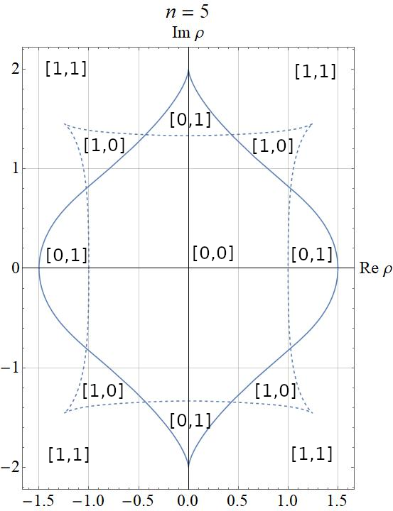
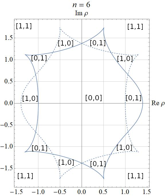
Figure 1. Closed curves $B_{n}^{(1)}$ (solid lines) and $B_{n}^{(2)}$ (dashed lines) for $n=5$ (left) and $n=6$ (right). The pairs of integers ($[1,0]$, $[0,0]$, etc.) denote the numbers of type-1 and type-2 extraordinary eigenvalues within the regions formed by $B_{n}^{(1)}$ and $B_{n}^{(2)}$.

5. Double eigenvalues and borderline-curve singularities

5.1. Locations of curve singularities

In Fig. 1, it is evident that $\rho=i2$ is a singular point of $B^{(1)}_{5}$, that $B^{(2)}_{6}$ presents a singularity in each of the four quadrants (the actual values of $\rho$ are $1.31\pm i1.12$ and $0.51\pm i1.74$), etc. For any $n$, Theorem 5.2 will enable a priori determination of all singularities in $\mathbb{C}\setminus\mathbb{R}$. Our theorem uses the usual definition [5] pertaining to parametrized curves, namely that singularities occur whenever $df_{n}^{(k)}(u)/du=0$. In this manner, Theorem 5.2 will demonstrate a one-to-one correspondence between the aforementioned singularities and the borderline/double eigenvalues of Definition 1.2. To begin with, Lemma 4.2(vi) and $v(n,u)\in\mathbb{R}$ imply an auxiliary result.

Lemma 5.1.

Let $u\in(-\pi,0)\cup(0,\pi)$, let $\mu(n,u)$ be determined via (4.2)–(4.4), and let $k=1$ or $k=2$. Then $df^{(k)}_{n}(u)/du=0$ iff $u$ is such that

(5.1) $$\frac{\sin[n\mu(n,u)]}{\sin\mu(n,u)}=\pm n,\quad\quad k=\left\{{1\atop 2}\right\}.$$

Our theorem follows by translating the conditions on $u$ into conditions on $\rho$ and invoking the definition of a curve singularity.

Theorem 5.2.

Let $k=1$ or $k=2$. The point $\rho_{0}\in\mathbb{C}\setminus\mathbb{R}$ is a singularity of $B^{(k)}_{n}$ iff $K_{n}(\rho_{0})$ possesses a type-$k$ borderline/double eigenvalue.

Proof.

Suppose that $\rho_{0}\in\mathbb{C}\setminus\mathbb{R}$ is a singular point of $B^{(k)}_{n}$, so that $\rho_{0}=f^{(k)}_{n}(u_{0})$ where $df^{(k)}_{n}(u_{0})/du=0$. Proposition 4.4(i) gives $\rho_{0}\neq\pm\xi_{n}$, $u_{0}\neq 0$, and $u_{0}\neq\pm\pi$. Lemma 5.1 then implies (5.1). We have thus found a $\mu$ for which equations (2.1) and (2.2) are satisfied, with the type-$k$ eigenvalue $\lambda$ equal to $-n$. By Corollary 3.3(iii), this means that $K_{n}(\rho_{0})$ possesses a type-$k$ borderline/double eigenvalue.

Conversely, suppose that $K_{n}(\rho_{0})$ possesses a type-$k$ borderline/double eigenvalue. Then $\rho_{0}\notin\mathbb{R}$ and $\lambda=-n$ by Corollary 3.3, so that (2.1) and (2.2) are satisfied for some $\mu$. As the magnitude of the eigenvalue $\lambda$ is $n$, we must have $\mu=\mu(n,u_{0})$ for some nonzero $u_{0}\in(-\pi,\pi)$, where $\mu(n,u_{0})$ is found via (4.2)-(4.4). Accordingly, (2.1) is the same as (5.1). Lemma 5.1 then gives $df^{(k)}_{n}(u_{0})/du=0$, completing our proof. ∎

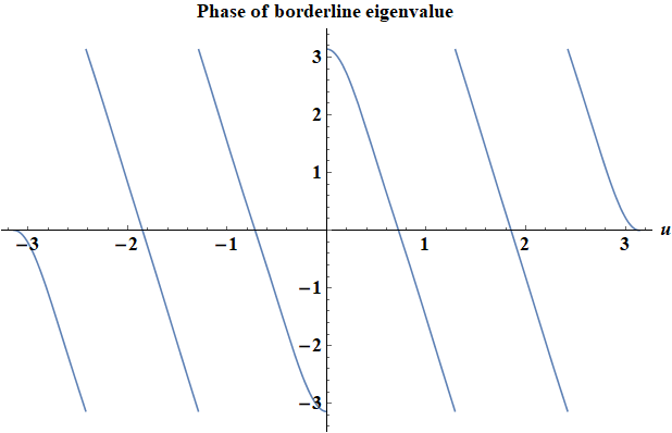
Figure 2. Phase (principal value) of type-1 borderline eigenvalue $\lambda=b_{6}^{(1)}(u)$ as function of $u$ for $n=6$. For $u\neq 0$, the four jumps signal the appearance of a borderline/double eigenvalue equal to $-6$. The jump at $u=0$ corresponds to a non-repeated eigenvalue equal to $-6$.

For $n=6$, Fig. 2 shows the (principal value of the) phase of the type-1 eigenvalue $\lambda=b_{n}^{(1)}(u)$ [see (4.1)] as a function of $u$. This is the phase of the borderline eigenvalue as we move along the borderline curve $B_{n}^{(1)}$. Discontinuities occur whenever $u=u_{0}$ is such that the phase jumps by $2\pi$, so that $b_{n}^{(1)}(u_{0})=-n=-6$. By Corollary 3.3(iii), this means that the borderline eigenvalue becomes a borderline/double eigenvalue, with the single exception of the case $u_{0}=0$, corresponding to $\rho_{0}=\xi_{n}=\xi_{6}=7/5$ [see (4.12), Remark 3.2, and the solid line in Fig. 1, right]. When $u_{0}=0$ the borderline eigenvalue equals $-n$, but this eigenvalue is not a borderline/double one. In all other cases, Theorem 5.2 tells us that $\rho_{0}=f_{n}^{(1)}(u_{0})$ is a singularity of $B_{n}^{(1)}$. These cases correspond to the four singularities, one in each quadrant, in the solid line in the right Fig. 1.

5.2. Cusp-like nature of curve singularities; local bisector

Let $\rho_{0}$ be any of the type-1 or type-2 singularities discussed in Theorem 5.2. Near $\rho=\rho_{0}$, the two coalescing eigenvalues $\lambda$ can be expanded into a Puiseux series [6]. The first two terms are

$$\lambda\cong-n+\eta_{0}(\rho-\rho_{0})^{1/2},$$

where the square root is double-valued. Let $\rho-\rho_{0}=r\,e^{i\theta}$ ($r\ll 1$) and $\eta_{0}=|\eta_{0}|\,e^{i\psi}$ so that

$$|\lambda|^{2}\cong n^{2}+|\eta_{0}|^{2}r-2n|\eta_{0}|\sqrt{r}\cos\left(\frac{\theta}{2}+\psi\right).$$

When $\rho$ is on the level curve $B_{n}^{(k)}$ we have $|\lambda|^{2}=n^{2}$ so that

(5.2) $$r=r(\theta)\cong\frac{2n^{2}}{|\eta_{0}|^{2}}\left[1+\cos(\theta+2\psi)\right],\quad r\ll 1.$$

Eq. (5.2) is a polar equation for a cardioid [7] that has a cusp at the origin $r=0$, or at $\rho=\rho_{0}$. This cardioid is bisected by the ray $\theta=\pi-2\psi$ which is tangent, at $\rho_{0}$, to the two arcs of the cardioid. Near $\rho=\rho_{0}$, the cardioid describes the local behavior of $B_{n}^{(k)}$. We thus use the terms cusp-like singularity for any of the $\rho_{0}$ of Theorem 5.2, and local bisector for the tangent ray passing through $\rho_{0}$.

Since cardioids are Jordan curves, the above result verifies Conjecture 4.5 locally near any cusp-like singularity, i.e., for all $u$ and $u^{\prime}$ such that $f_{n}^{(k)}(u)$ and $f_{n}^{(k)}(u^{\prime})$ are sufficiently close to the singularity.

It is possible to determine the $k$-dependent parameters $|\eta_{0}|$ and $\psi$. Without dwelling on this, we mention that: (i) $B_{n}^{(1)}$ and $B_{n}^{(2)}$ each have two cusps on the imaginary axis when $n=5,9,13,\ldots$ and $n=3,7,11,\ldots$, respectively, see the example in the left Fig. 1; (ii) the corresponding local bisectors also lie on the imaginary axis.

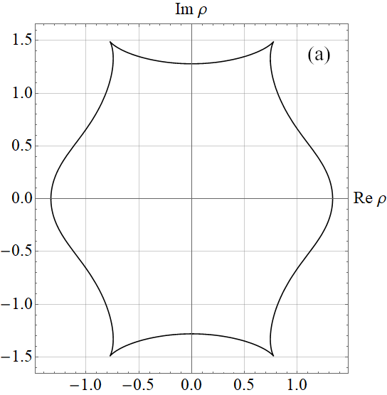
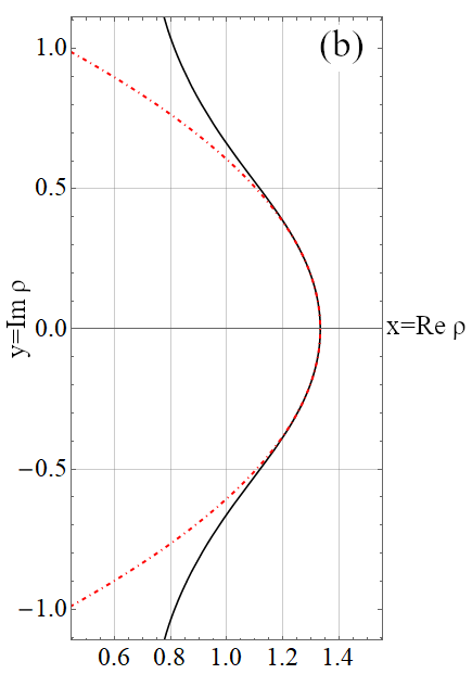
Figure 3. (a) Closed curve $B_{n}^{(1)}$ in the $\rho$-plane for $n=7$. (b) Focus on the region around $\xi_{7}=4/3$ of the curve $B_{n}^{(1)}$ (solid line). The dot-dashed curve is the parabola of (5.8) for $n=7$.

5.3. Parabolic behaviors near real axis

Recall that there are no borderline/double eigenvalues when $\rho\in\mathbb{R}$, and that Sections 5.1 and 5.2 left out the curve-intersections with the real axis. We thus proceed to Taylor-expand $f^{(k)}_{n}(u)$ about $u=0$ (formulas for $u=\pi$ then follow from the symmetries listed in Proposition 4.4). To carry this out, we assume a small-$u$ expansion of $v(n,u)$ of the form

$$v(n,u)=\alpha u\left[1+\beta u^{2}+\gamma u^{4}\right],\quad u\rightarrow 0+0,\quad\alpha>0,$$

substitute into the left-hand side of (4.3), Taylor-expand the right-hand side $g_{n}(u)$ using (4.4), equate the coefficients of the resulting powers of $u$ (namely of $u^{4}$, $u^{6}$, and $u^{8}$), and solve for $\alpha$, $\beta$, and $\gamma$. The result of this procedure is

(5.3) $$v(n,u)=u\left[1-\frac{n^{2}+1}{15}u^{2}+\frac{(n^{2}+1)^{2}}{150}u^{4}+O(u^{6})\right],\quad u\rightarrow 0+0.$$

In this manner, we have determined an approximation to $v(n,u)$ that satisfies (4.3) to $O(u^{10})$. The number of terms in (5.3) is sufficient to obtain (nonzero) small-$u$ approximations to the real and imaginary parts of $f^{(1)}_{n}(u)-\xi_{n}$ and $f^{(2)}_{n}(u)-1$: Substitution of (5.3) into (4.1) and (4.5) gives

(5.4) $$f_{n}^{(1)}(u)=\xi_{n}\left\{1-\frac{in}{3}u^{2}-n\left[\frac{n^{2}+5n+1}{90}-i\frac{n^{2}+1}{45}\right]u^{4}+O(u^{6})\right\},\quad u\rightarrow 0+0$$

and

(5.5) $$f_{n}^{(2)}(u)=1-inu^{2}+n\left[\frac{n^{2}-5n+1}{10}+i\frac{n^{2}+1}{15}\right]u^{4}+O(u^{6}),\quad u\rightarrow 0+0.$$

Let $x={\rm Re}\rho$ and $y={\rm Im}\rho$. Consistent with Lemma 4.2(v), the approximations to $y$ in (5.4) and (5.5) are negative, corresponding to the lower-half plane. By Proposition 4.4(ii), we can obtain an upper-half plane approximation to $y$ by using the opposite sign. Consequently, our final parametrized (small-$u$) results for the behaviors of $B_{n}^{(k)}$ near the positive real semi-axis are

(5.6) $$B_{n}^{(1)}:\quad x-\xi_{n}\simeq-\xi_{n}\frac{n(n^{2}+5n+1)}{90}u^{4},\quad y\simeq\pm\xi_{n}\frac{n}{3}u^{2},\qquad\rho\rightarrow\xi_{n},$$

(5.7) $$B_{n}^{(2)}:\quad x-1\simeq\frac{n(n^{2}-5n+1)}{10}u^{4},\quad y\simeq\pm nu^{2},\qquad\rho\rightarrow 1,$$

where, as already mentioned, the upper signs correspond to $u<0$. In Cartesian coordinates, it follows that our curves locally behave like parabolas according to

(5.8) $$B_{n}^{(1)}:\quad y^{2}\simeq\frac{10n\xi_{n}}{n^{2}+5n+1}(\xi_{n}-x)\qquad x\rightarrow\xi_{n}-0,$$

(5.9) $$B_{n}^{(2)}:\quad y^{2}\simeq\begin{cases}\displaystyle\frac{10n}{|n^{2}-5n+1|}(1-x),\quad n=2,3,4;\quad x\rightarrow 1-0\\ \displaystyle\frac{10n}{n^{2}-5n+1}(x-1),\quad n=5,6,7,\ldots\quad x\rightarrow 1+0.\end{cases}$$

Fig. 3 depicts representative numerical results.

6. Extraordinary eigenvalues

This section deals with extraordinary type-1 (or type-2) eigenvalues. Some of our results assume that that Conjecture 4.5 is true, while others do not.

6.1. On the number of extraordinary eigenvalues

If the closed curves $B_{n}^{(1)}$ and $B_{n}^{(2)}$ are indeed Jordan (Conjecture 4.5), then each curve separates the complex-$\rho$ plane into two open and pathwise-connected components, namely an interior and an exterior.

Conditional Proposition 6.1.

Assume that Conjecture 4.5 is true, so that $B_{n}^{(k)}$ possesses an interior $I_{n}^{(k)}$ and an exterior $E_{n}^{(k)}$ ($k=1,2$). Let $\rho\in\mathbb{C}$, and let $j_{n}^{(k)}(\rho)$ denote the number, counting multiplicities, of type-$k$ extraordinary eigenvalues of $K_{n}(\rho)$. Then all extraordinary eigenvalues are non-repeated, and

(6.1) $$j_{n}^{(k)}(\rho)=\begin{cases}0,{\rm\,if\,\,}\rho\in I_{n}^{(k)}\\ 0,{\rm\,if\,\,}\rho\in B_{n}^{(k)}\\ 1,{\rm\,if\,\,}\rho\in E_{n}^{(k)}\end{cases}.$$

Proof.

Imagine moving along any (continuous) path in the complex $\rho$-plane. Along the path, the eigenvalues of $K_{n}(\rho)$ vary continuously. Consequently, the integer-valued function $j_{n}^{(k)}(\rho)$ can be discontinuous at $\rho=\rho_{0}$ only if some eigenvalue of $K_{n}(\rho_{0})$ is borderline, i.e., some eigenvalue’s magnitude assumes the value $n$ when $\rho=\rho_{0}$. According to Corollary 4.3, this can happen only if $\rho_{0}\in B_{n}^{(k)}$. Therefore, $j_{n}^{(k)}(\rho)$ remains unaltered along any path lying entirely within $I_{n}^{(k)}$. Since any two points in $I_{n}^{(k)}$ can be joined by such a path (lying entirely within $I_{n}^{(k)}$), $j_{n}^{(k)}(\rho)$ is constant within $I_{n}^{(k)}$. Similarly, $j_{n}^{(k)}(\rho)$ is constant within $E_{n}^{(k)}$. We thus proceed to find $j_{n}^{(k)}(\rho)$ for one point $\rho$ within $I_{n}^{(k)}$ and for one point $\rho$ within $E_{n}^{(k)}$.

By Proposition 4.4(i), the positive real semi-axis intersects $B_{n}^{(1)}$ at $\rho=\xi_{n}$ and at no other point; and it intersects $B_{n}^{(2)}$ at $\rho=1$ and at no other point. We have thus found a point $\rho$ in each region,

(6.2) $$0\in I_{n}^{(1)},\qquad 0\in I_{n}^{(2)},\qquad\xi_{n}+1\in E_{n}^{(1)},\qquad 2\in E_{n}^{(2)},$$

and Table 1 of Proposition 1.3 gives the corresponding $j_{n}^{(k)}(\rho)$ as

(6.3) $$j_{n}^{(1)}(0)=0,\qquad j_{n}^{(2)}(0)=0,\qquad j_{n}^{(1)}(\xi_{n}+1)=1,\qquad j_{n}^{(2)}(2)=1.$$

Both for $k=1$ and $k=2$, we have now shown that $j_{n}^{(k)}(\rho)=0$ and $j_{n}^{(k)}(\rho)=1$ whenever $\rho\in I_{n}^{(k)}$ and $\rho\in E_{n}^{(k)}$, respectively.

Now consider a path that lies entirely within $I_{n}^{(k)}$, with the single exception of an endpoint that lies on $B_{n}^{(k)}$. Such a path will also leave $j_{n}^{(k)}(\rho)$ unaltered, because borderline eigenvalues are ordinary eigenvalues by definition. Thus $j_{n}^{(k)}(\rho)=0$ for all $\rho\in B_{n}^{(k)}$.

The integer $j_{n}^{(k)}(\rho)$, which equals the number of type-$k$ extraordinary eigenvalues of $K_{n}(\rho)$, counts double type-$k$ eigenvalues twice by definition. As $j_{n}^{(k)}(\rho)$ is at most 1, all extraordinary eigenvalues are non-repeated. ∎

Remark 6.2.

Suppose that Conjecture 4.5 is not true, and that there exist $B_{n}^{(k)}$ that separate the plane into more than two components, with all components open, disjoint, and pathwise connected. For any such $B_{n}^{(k)}$, let $E_{n}^{(k)}$ denote the component that extends to infinity and let $O_{n}^{(k)}$ denote the component that includes the origin. Then it is still true that

(6.4) $$j_{n}^{(k)}(\rho)=\begin{cases}0,{\rm\,if\,\,}\rho\in O_{n}^{(k)}\\ 1,{\rm\,if\,\,}\rho\in E_{n}^{(k)},\end{cases}$$

where, as before, $j_{n}^{(k)}(\rho)$ denotes the number of extraordinary eigenvalues of $K_{n}(\rho)$. To prove (6.4), it is only necessary to replace $I_{n}^{(k)}$ by $O_{n}^{(k)}$, $\xi_{n}+1$ by $\rho^{(1)}$, and $2$ by $\rho^{(2)}$ in the relevant part of the proof of Conditional Proposition 6.1, where $\rho^{(1)}$ and $\rho^{(2)}$ are sufficiently large positive numbers. Note that (6.4) makes no statement about $B_{n}^{(k)}$.

The numerically-generated curves in Fig. 1 intersect, thus forming a number of regions. We have labeled each region by the pair $\left[j_{n}^{(1)}(\rho),j_{n}^{(2)}(\rho)\right]$, where $j_{n}^{(k)}(\rho)$ corresponds to all interior points of the region. For example, the triangularly shaped region in the southeastern part of the left figure is labeled $[1,0]$ because all points $\rho$ interior to this region belong to $E_{5}^{(1)}$ and $I_{5}^{(2)}$. For any such $\rho$, $K_{5}(\rho)$ has one and only one extraordinary eigenvalue; and this eigenvalue is of type-1. The labels in Fig. 1 can be compared to the numbers (0 or 1) in Table 1 of Proposition 1.3.

6.2. Crossing the borderline

Let us still assume that Conjecture 4.5 is true. Besides those used in the proof of Conditional Proposition 6.1, it is instructive to consider paths that start in $I^{(k)}_{n}$, end in $E^{(k)}_{n}$, and cross $B^{(k)}_{n}$ once, say at a point $\rho=C$. Let us for definiteness take $k=1$. Although $j_{n}^{(1)}(\rho)$ always increases by $1$ as we move past $C$, this can occur in several ways:

(i) $C$ is not a cusp-like singularity and $C$ does not belong to $B^{(2)}_{n}$ (i.e., $C$ does not concurrently belong to the other borderline curve): In this case, upon moving past $C$, the magnitude of a type-1 simple eigenvalue exceeds the threshold $n$. By Conditional Proposition 4.6, there is a unique such eigenvalue. Furthermore, no other eigenvalue, of either type, reaches the threshold.

(ii) $C\in B^{(1)}_{n}\cap B^{(2)}_{n}$ (for definiteness, let the path start in $I_{n}^{(1)}\cap I_{n}^{(2)}$ and end in $E_{n}^{(1)}\cap E_{n}^{(2)}$): Now, the magnitudes of two simple eigenvalues—one of each type—simultaneously exceed the threshold when we move past $C$, so that $[j_{n}^{(1)},j_{n}^{(2)}]$ changes from $[0,0]$ to $[1,1]$. This case can be visualized via the examples in Fig. 1.

(iii) $C$ is a cusp-like singularity, corresponding to a borderline/double type-1 eigenvalue. (The crossing path can, for example, be the local bisector discussed in Section 5.2.) The fact that $j_{n}^{(1)}(\rho)$ increases by one [rather than two, see (6.1)] implies that only one eigenvalue crosses the threshold. This must mean that a second eigenvalue reaches the threshold, but then turns back without crossing. This situation, which is reminiscent of bifurcations in a number of physical problems—see, for example, the exceptional points of [8], [9], [10]—is illustrated for two cases in Fig. 4.

In the top figure [Fig. 4(a)], a fine zoom (not shown here for brevity) revealed that the line to the left of the cusp-like singularity (i.e., the seemingly single line corresponding to $d<0$) is actually two lines, corresponding to two different eigenvalues of nearly equal magnitudes.

Fig. 4(b) is like Fig. 4(a) except that $n$ is much larger (95 instead of 7), $C$ is purely imaginary, and $C$ belongs to $B_{n}^{(2)}$ rather than $B_{n}^{(1)}$. This time, movement along the local bisector means that we are on the imaginary axis which, by Proposition 4.4(iv), bisects the entire curve $B_{n}^{(2)}$. When $\rho$ is purely imaginary and $n=3,5,\ldots$, it is a corollary of Lemma 2.2 that the type-2 eigenvalues of $K_{n}(\rho)$ either are real, or come in complex-conjugate pairs (similarly to the roots of a polynomial with real coefficients). In Fig. 4(b) it is evident that both these situations occur: For $d<0$ there are two conjugate eigenvalues while, for $d>0$, there are two real and unequal eigenvalues. In other words, the single line to the left of $d=0$ represents the exactly-coinciding magnitudes of two complex-conjugate eigenvalues, while the two lines to the right correspond to two real eigenvalues of diverging magnitudes and of phases initially ($d=0$) equal to $\pi$. In fact, both eigenvalues remain negative for all $d\geq 0$. If we proceed along the positive imaginary semi-axis [beyond the movement depicted in Fig. 4(b)] we will find that the extraordinary eigenvalue will asymptotically approach $\rho^{n-1}=-|\rho|^{94}$ and that the ordinary one will tend to the limit $-1$. Eqn. (6.6) below theoretically verifies these two numerical results.

Apart from Fig. 4, we checked all predictions of Sections 6.1 and 6.2 numerically. Many such tests can serve as indirect corroborations of Conjecture 4.5.

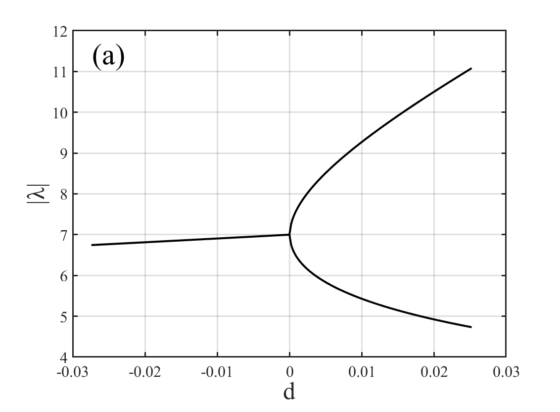
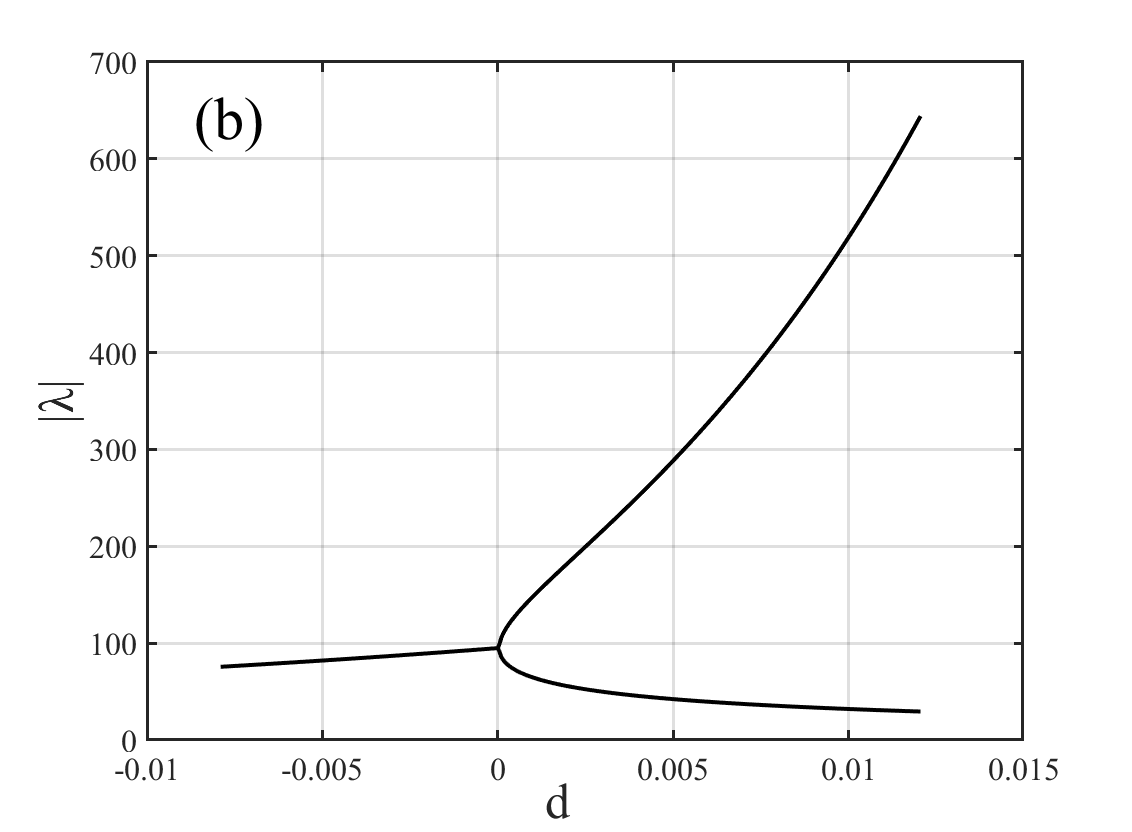
Figure 4. (a) Modulus of the two type-1 eigenvalues whose magnitudes are close to $n$, for $n=7$, as a function of the distance $d$ to the cusp-like singularity at $C=0.77570-i1.49222$. Movement is along the local bisector. The region inside (outside) the curve corresponds to $d<0$ ($d>0$), with $d=0$ at the singularity. (b) As in (a), but with $n=95$, type-2 eigenvalues, and $C=i1.06795$; here, movement is along the imaginary axis, which underlies the local bisector.

6.3. The limit $|\rho|\rightarrow\infty$

For the case where $|\rho|$ is sufficiently large, we now—without assuming Conjecture 4.5—obtain large-$|\rho|$ approximations [eqns. (6.6) below] to all eigenvalues, valid for any phase of $\rho$.

Denote the solutions to the two equations in (2.2) by $\pm\mu_{m}$, where an odd (even) index $m$ corresponds to the first (second) equation, corresponding to the type-1 (type-2) case. The $\pm$ sign is irrelevant to the eigenvalues we wish to determine. Via (2.2), we can easily justify the following large-$|\rho|$ approximations:

(6.5) $$\mu_{m}\sim\begin{cases}\displaystyle i\ln\rho,{\rm\,if\,\,}m=0\\ \displaystyle i\ln\rho,{\rm\,if\,\,}m=1\\ \displaystyle\frac{(k-1)\pi}{n-1},{\rm\,if\,\,}m=2,3,\ldots,n-1\end{cases}\quad|\rho|\rightarrow\infty.$$

In (6.5), the large-$|\rho|$ solutions $\mu_{2},\mu_{3},\ldots,\mu_{n-1}$ correspond to zeros of the denominator of (2.2). By contrast, $\mu_{0}$ and $\mu_{1}$ result from seeking large-$|\rho|$ solutions such that numerator and denominator have the same order of magnitude. The polynomial formulation of Sections 3 and 4 of [1] readily ensures that we have found as many solutions to (2.2) as are necessary to correspond to all eigenvalues.

Denote the corresponding to $\mu_{m}$ eigenvalue by $\lambda_{m}$, so that an odd (even) index $m$ corresponds to a type-1 (type-2) eigenvalue. Via (6.5) and (2.1) we obtain

(6.6) $$\lambda_{m}\sim\begin{cases}\rho^{n-1},{\rm\,if\,\,}m=0\\ -\rho^{n-1},{\rm\,if\,\,}m=1\\ -1,{\rm\,if\,\,}m=2,3,\ldots,n-1\end{cases}\quad|\rho|\rightarrow\infty,$$

where, for the cases $m=0$ and $m=1$, we have retained the leading term only. Note that (6.6) predicts $\lambda_{0}\lambda_{1}\ldots\lambda_{n-1}\sim(-1)^{n-1}\rho^{2n-2}$, consistent with the fact [1] that the determinant of $K_{n}(\rho)$ equals $(1-\rho^{2})^{n-1}$. Note also that the large-$n$ formulas for $\lambda_{0}$ and $\lambda_{1}$ in Section 5 of [1] reduce, as $|\rho|\rightarrow\infty$, to the corresponding formulas in (6.6); this explains why we obtain good numerical agreement even in cases where $\rho$ and $n$ are both large.

Remark 6.2 showed that for all sufficiently large $|\rho|$, there are exactly two extraordinary eigenvalues, one of each type. Eqn. (6.6) further shows that, asymptotically, these eigenvalues ($\lambda_{0}$ and $\lambda_{1}$) are equal to plus/minus the largest element of $K_{n}(\rho)$. Numerically, (6.6) can give very good results. When, for example, $\rho=15+i12$ and $n=6$, (6.6) gives three-digit accuracy for the real parts of $\lambda_{0}$ and $\lambda_{1}$, and two-digit accuracy for the (smaller) imaginary parts. As for the remaining (ordinary) eigenvalues, the one furthest from $-1$ is approximately $-1.07+i0.05$. Since the matrix elements vary greatly in magnitude when $|\rho|$ is large (this is especially true when $n$ is also large), eqn. (6.6) can also be useful for numerical computations.

References

- [1] G. Fikioris, Spectral properties of Kac–Murdock–Szegő matrices with a complex parameter, Linear Algebra Appl. 553 (2018), 182–210.
- [2] W. F. Trench, Asymptotic distribution of the spectra of a class of generalized Kac–Murdock–Szegő matrices, Linear Algebra Appl. 294 (1999), 181–192; see also Erratum: W. F. Trench, Linear Algebra Appl. 320 (2000) 213.
- [3] W. F. Trench, Spectral distribution of generalized Kac–Murdock–Szegő matrices, Linear Algebra Appl. 347 (2002), 251-273.
- [4] J. M. Bogoya, A. Böttcher, S. M. Grudsky, Eigenvalues of Toeplitz matrices with polynomial increasing entries, J. Spectr. Theory 2 (2012) 267-292.
- [5] E. Kreyszig, Differential geometry, Dover Publications, New York, 1991.
- [6] P. Lancaster and M. Tismenetsky, The theory of matrices; 2nd Ed., with applications. Academic Press, Inc., San Diego, CA, 1985.
- [7] J. D. Lawrence, A catalog of special plane curves, Dover, New York, 1972, pp. 118-119.
- [8] M.-A. Miri, A. Alù, Exceptional points in optics and photonics, Science 363 (2019) DOI: 10.1126/science.aar7709.
- [9] M. A. K. Othman, V. Galdi, G. Capolino, Exceptional points of degeneracy and symmetry in photonic coupled chains of scatterers, Phys. Rev. B, 95 (2017), 104305.
- [10] M. A. K. Othman and F. Capolino, Theory of exceptional points of degeneracy in uniform coupled waveguides and balance of gains and loss, IEEE Trans. Antennas Propagat., 65 (2017), pp. 5289–5302.