The Onsager-Machlup Function as Lagrangian for the Most Probable Path of a Jump-Diffusion Process

Abstract

This work is devoted to deriving the Onsager-Machlup function for a class of stochastic dynamical systems under (non-Gaussian) Lévy noise as well as (Gaussian) Brownian noise, and examining the corresponding most probable paths. This Onsager-Machlup function is the Lagrangian giving the most probable path connecting metastable states for jump-diffusion processes. This is done by applying the Girsanov transformation for measures induced by jump-diffusion processes. Moreover, we have found this Lagrangian function is consistent with the result in the special case of diffusion processes. Finally, we apply this new Onsager-Machlup function to investigate dynamical behaviors analytically and numerically in several examples. These include the transitions from one metastable state to another metastable state in a double-well system, with numerical experiments illustrating most probable transition paths for various noise parameters.

Keywords: Onsager-Machlup action functional; noise-induced transition paths; jump-diffusion processes; stable Lévy noise; Lagrangian; most probable paths.

1 Introduction

A diffusion process is usually a solution process of a differential equation driven by Brownian motion. The Onsager-Machlup (OM) function of a diffusion process was first introduced in [21] and also considered in [26, 10], among many more recent efforts. It appears in the asymptotic probability estimation of sample paths of a diffusion process lying within a tube along a smooth path. In fact, this asymptotic likelihood contains an exponential term whose exponent is a negative integral over a time interval, and the integrand in this integral is the so-called OM function. For convenience, we also call the integral of OM function over a time interval the OM action functional. In other words, the OM function helps to evaluate the asymptotic probability measure of a small neighborhood of a smooth path. Taking the idea of Dürr and Bach [10], another more physical meaning can be given to the OM function, which interprets the OM function as a Lagrangian for determining the most probable tube of a diffusion process by means of a variation principle. Thus, the OM function serves as a tool to study some dynamical behaviors of stochastic dynamical systems, such as most probable transition paths connecting metastable states.

The method concerning the derivation of the OM function for a diffusion process has been developed in the preceding years. Onsager and Machlup [21] were the first to derive the OM function for diffusion processes with linear drift and constant diffusion coefficients. Subsequently, Tisza and Manning [28] began to generalize the results of [21] to nonlinear equations. Takahashi-Watanabe [29] and Fujita-Kotani [12] further derived OM function for Brownian motion on a complete Riemannian manifold. Another purely probabilistic proof of Onsager-Machlup formula for diffusion processes on a Riemannian manifold was given by Hara and Takahashi [14]. There are other works devoted to deriving the OM functions for diffusion processes using various approaches [26, 3, 10]. For example, Dürr and Bach [10] derived the OM function based on the Girsanov transformation for measures induced by diffusion processes (see also [18]). In addition, an application concerned with the fluctuation phenomena is described by Singh [25] and Deza et al [7]. More recently, OM function has been used to analyze issues related to the trajectory entropy of the overdamped Langevin equation [13] as well as to data assimilation [27, 6]. Note that most existing works mentioned above are for diffusion processes, i.e. solution processes of stochastic differential equations with (Gaussian) Brownian motion.

However, random fluctuations in complex biological and physical systems are often non-Gaussian rather than Gaussian [34, 32, 31]. Lévy motions are appropriate models for a class of important non-Gaussian processes with jumps or bursts [5]. In the sense of Lévy-Itô decomposition, a general Lévy motion could be understood as a sum of a Brownian motion and a pure jump Lévy motion, in addition to a drift term which may be absorbed in the vector field in stochastic differential equation (SDE) models for these complex systems. Note that Ditlevsen [8] found that a climate change system may be modelled by an SDE with Brownian motion and Lévy motion, and an objective is to understand climate transitions between climate metastable states. An SDE with Brownian motion and Lévy motion also appeared for modeling certain gene transcriptions in biology [34], with a goal to quantify the transitions between low and high protein concentrations. Motivated by these modelling efforts, we plan to investigate transition phenomena for these non-Gaussian complex systems. Especially, it is desirable to consider the OM functions for jump-diffusion processes, defined as solution processes of stochastic differential equations with Brownian motion $B_{t}$ and Lévy motion $L_{t}$, and examine the corresponding most probable paths between metastable paths. As far as we know, this is not yet done.

We remark that Moret and Nualart [19] recently derived the OM function for the fractional (but still Gaussian) Brownian motion. Bardina et al [4] dealt with the asymptotic evaluation of the Poisson measure for a tube around a jump path but that work is not for a general Lévy motion.

In this present paper, we consider a class of one-dimensional nonlinear stochastic dynamical systems with Brownian noise and Lévy noise. The solution process is a jump-diffusion process. Using the Girsanov transformation for a measure induced by this jump-diffusion process, we derive the Onsager-Machlup function, which may still be regarded as the Lagrangian giving the most probable tube around a smooth path as in the case of diffusion processes [10]. Different from the case of diffusion processes, an extra term depicting the impact of Lévy noise will appear in the OM function. It is worthwhile to mention that our result is consistent with the result of the diffusion processes [21, 10, 3] in the absence of Lévy noise. Thus, our work extracts the non-trivial effect of pure jump Lévy noise in stochastic dynamics and we will see that this will affect the most probable paths. With the help of OM function and a variation principle, the most probable path from one state to another, especially the most probable path from one metastable state to another metastable state over a finite time interval, for some stochastic dynamical systems can be found by numerical simulation. We will illustrate this for a stochastic system with linear potential and a prototypical double-well system under Lévy noise and Brownian noise.

An inspiration for this paper goes back to the work [10] by Dürr and Bach. We generalize and improve their results to a class of dynamical systems under random fluctuations consisting of Brownian noise and Lévy noise. This will give rise to several difficulties both in analytic and probabilistic aspects as the non-Gaussian pure jump Lévy noise is present. In addition, we use the same notations as in [10] to compare our results with the diffusion case.

This paper is organized as follows. In Section 2, we recall some basic concepts about Lévy motions, and present the framework for deriving the OM function of a stochastic dynamical system. After setting up the theory of induced measures in Section 3, we derive the OM function in Section 4. Subsequently in Section 5, we present the equation of motion for the most probable path of a class of jump-diffusion processes and discuss its solutions. Some concrete examples are tested to illustrate our results in Section 6. Finally, we summarize our work in Section 7.

2 Preliminaries

We now recall some basic facts about Lévy motions [1, 23, 9], introduce a class of stochastic differential equations to be studied, and define the OM function and OM functional.

2.1 Lévy motions

Let $(\Omega,\mathcal{F},(\mathcal{F}_{t})_{t\geq 0},\mathds{P})$ be a filtered probability space, where $\mathcal{F}_{t}$ is a nondecreasing family of sub-$\sigma$-fields of $\mathcal{F}$ satisfying the usual conditions. An $\mathcal{F}_{t}$-adapted stochastic process $L_{t}=L(t)$ taking values in $\mathbb{R}^{n}$ with $L(0)=0$ $a.s.$ is called a Lévy motion if it is stochastically continuous, with independent increments and stationary increments.

An $n$-dimensional Lévy motion can be characterized by a drift vector $b\in\mathbb{R}^{n}$, an $n\times n$ non-negative-definite, symmetric matrix Q, and a Borel measure $\nu$ defined on ${\mathbb{R}^{n}}\backslash\{0\}$. We call $(b,Q,\nu)$ the generating triplet of the Lévy motion $L_{t}$. Moreover, we have the following Lévy-Itô decomposition for $L_{t}$:

$${L_{t}}=bt+B_{Q}(t)+\int_{|x|<1}x\tilde{N}(t,dx)+\int_{|x|\geq 1}xN(t,dx),$$

where $N(dt,dx)$ is the Poisson random measure on $\mathbb{R}^{+}\times({\mathbb{R}^{n}}\backslash\{0\})$, $\tilde{N}(dt,dx)=N(dt,dx)-\nu(dx)dt$ is the compensated Poisson random measure, $\nu(A)=EN(1,A)$ with $A\in\mathcal{B}({\mathbb{R}^{n}}\backslash\{0\})$ is the jump measure, and $B_{Q}(t)$ is an independent $n$-dimensional Brownian motion with covariance matrix $Q$. Here $|\cdot|$ denotes the Euclidean norm.

A scalar $\alpha$-stable Lévy motion $L_{t}^{\alpha,\beta}$ is a special Lévy motion, with non-Gaussianity index (or stability index) $\alpha\in(0,2)$ and skewness parameter $\beta\in[-1,1]$. It has the generating triplet $(b,0,\nu_{\alpha,\beta})$. Its jump measure $\nu_{\alpha,\beta}$ is in the form of

$$\nu_{\alpha,\beta}(d\xi)=c_{1}|\xi|^{-1-\alpha}\chi_{(0,\infty)}(\xi)d\xi+c_{2}|\xi|^{-1-\alpha}\chi_{(-\infty,0)}(\xi)d\xi$$

with $\beta=\frac{c_{1}-c_{2}}{c_{1}+c_{2}}$, $c_{1}=k_{\alpha}\frac{1+\beta}{2}$, and $c_{2}=k_{\alpha}\frac{1-\beta}{2}$, where

$$k_{\alpha}=\left\{\begin{array}[]{ll}\frac{\alpha(1-\alpha)}{\Gamma(2-\alpha)\cos(\frac{\pi\alpha}{2})},&\hbox{if $\alpha<1$,}\\ \frac{2}{\pi},&\hbox{if $\alpha=1$.}\end{array}\right.$$

Here, $\chi(\xi)$ denotes indicator function and $\Gamma$ is the Gamma function. If drift vector $b=0$, and $\nu_{\alpha,\beta}$ is symmetric, i.e. $\beta=0$, then this stable process is called a symmetric $\alpha$-stable process. Note that $\int_{|\xi|<1}|\xi|\nu_{\alpha,\beta}(d\xi)$ is finite if and only if $\alpha<1$ and the integral $\int_{|\xi|\geq 1}|\xi|\nu_{\alpha,\beta}(d\xi)$ is finite if and only if $\alpha>1$.

2.2 Framework

Consider the following scalar stochastic differential equation (SDE) defined on $\tau=[s,u]$ with respect to $(\Omega,\mathcal{F},(\mathcal{F}_{t})_{t\geq 0},\mathds{P})$

$$\begin{split}&dX_{t}=f(X_{t-})dt+g(X_{t-})dB_{t}+dL_{t},\\ &X_{s}=x_{0}\in\mathbb{R}.\end{split}$$ (2.1)

Where ${L_{t}}$ is a Lévy process with characteristics $(0,0,\nu)$ satisfying $\int_{|\xi|<1}\xi\nu(d\xi)<\infty$, $B_{t}$ is a standard Brownian motion and $X_{t-}$ is the left limit at the point $t$, i.e. $X_{t-}=\lim_{s\uparrow t}X_{s}$.

More precisely, the above equation can be written in the following form by employing the Lévy-Itô decomposition :

$$\begin{split}&dX_{t}=f(X_{t-})dt+g(X_{t-})dB_{t}+\int_{|x|<1}x\tilde{N}(dt,dx)+\int_{|x|\geq 1}xN(dt,dx),\\ &X_{s}=x_{0}\in\mathbb{R}.\end{split}$$

The last term in the preceding equation involves large jumps that are controlled by $x$. This term can be handled by using interlacing [1, Page 365], and it makes sense to begin by omitting this term and concentrate on the study of the equation driven by continuous noise interspersed with small jumps. To this end, we consider the following SDE:

$$\begin{split}&dX_{t}=f(X_{t-})dt+g(X_{t-})dB_{t}+\int_{|x|<1}x\tilde{N}(dt,dx),\\ &X_{s}=x_{0}\in\mathbb{R}.\end{split}$$ (2.2)

If we further assume that $f(x)$ and $g(x)$ are locally Lipschitz continuous functions and satisfy “one sided linear growth” condition in the following sense:

C1 (Locally Lipschitz condition) For any $R>0$, there exists $K_{1}>0$ such that, for all $|y_{1}|,|y_{2}|\leq R$,

$$|f(y_{1})-f(y_{2})|^{2}+|g(y_{1})-g(y_{2})|^{2}\leq K_{1}|y_{1}-y_{2}|^{2},$$

C2 (One sided linear growth condition) There exists $K_{2}>0$ such that, for all $y\in\mathbb{R}$,

$$|g(y)|^{2}+2y\cdot f(y)\leq K_{2}(1+|y|^{2}),$$

then there exists a unique global solution to (2.2) and the solution process is adapted and càdlàg, refer to Theorem 3.1 of [2], or [33]. We call a solution of (2.2) a jump-diffusion process. As we see, it happens to be a diffusion process only in the absence of Lévy noise. And note that there is by no means universal agreement about the use of the phrase jump-diffusion process. Thus, it makes sense to use this terminology to denote the solution of (2.2) throughout the paper [1, Page 383].

Now we will introduce some notations and terminologies to be used throughout the paper. Denote by $C^{1}(\mathbb{R})$ the set of all real-valued continuous differentiable functions, $C^{2}(\mathbb{R})$ the set of all real-valued twice continuous differentiable functions and $H^{1}([s,u];\mathbb{R})$ the set of all real-valued square integrable functions with square integrable weak derivative defined on $\tau=[s,u]$. Denote the space of paths of a solution process of (2.2) by $D_{\tau}^{x_{0}}$, which is the space of càdlàg functions, i.e.,

$$D_{\tau}^{x_{0}}=\{x(t)\mid x:\tau\rightarrow\mathbb{R},x(t)\hbox{ continuous from the right and have limits on the left},x(s)=x_{0}\}.$$

For each finite subset $S$ of $[s,u]$ write $\pi_{S}$ for the projection map from $D_{\tau}^{x_{0}}$ into $\mathbb{R}^{S}$ that takes an $x$ onto its vector of values $\{x(t):t\in S\}$. These projections generate the projection $\sigma$-field $\mathcal{P}$. The measurability in this paper will always refer to this $\sigma$-field.

As every càdlàg function on $\tau$ is bounded, equipping $D_{\tau}^{x_{0}}$ with the uniform norm $\|\cdot\|$

$$\|x\|=\sup_{t\in[s,u]}|x(t)|,x(t)\in D_{\tau}^{x_{0}},$$

$D_{\tau}^{x_{0}}$ is a Banach space. No other norm will be used for $D_{\tau}^{x_{0}}$ in this paper. We could show that the $\sigma$-field $\mathcal{B}_{0}$ generated by closed balls for uniform norm is the projection $\sigma$-field $\mathcal{P}$, but not the larger Borel $\sigma$-field $\mathcal{B}_{\tau}^{x_{0}}$. For more details, see [22, Page 87-90].

Lemma 2.1.

$\mathcal{B}_{0}=\mathcal{P}$ and $\mathcal{P}\subsetneqq\mathcal{B}_{\tau}^{x_{0}}.$

Proof.

Consider a closed ball $B_{\rho}=\{y\in D_{\tau}^{x_{0}}:\sup_{t\in[s,u]}|y_{t}-z_{t}|\leq\rho\}$, where $z$ is an element of $D_{\tau}^{x_{0}}$. Since the functions in $D_{\tau}^{x_{0}}$ are right-continuous,

$$B_{\rho}={\cap}_{t_{k}}\{y\in D_{\tau}^{x_{0}}:|y_{t_{k}}-z_{t_{k}}|\leq\rho\}\in\mathcal{P},$$

where $t_{k}$ are the rational points of $[s,u]$. Therefore $\mathcal{B}_{0}\subset\mathcal{P}$. Conversely, we can express $B=\{x:x_{t}>a\}$ as a countable union of closed balls. Thus $\mathcal{B}_{0}$=$\mathcal{P}$.

Consider a cylinder set $B=\{x:x_{t_{1}}<b\}$. For every $x\in B$, we have $x_{t_{1}}\leq b-\epsilon$ where $\epsilon$ can be chosen sufficiently small. We find that there exists a neighborhood of $x$, denoted by $K(x,\epsilon)=\{y\in D_{\tau}^{x_{0}}\mid\|x-y\|<\epsilon,\epsilon>0\}$. For every $y\in K(x,\epsilon)$, $|y_{t_{1}}-x_{t_{1}}|\leq\parallel y-x\parallel<\epsilon$, i.e. $y_{t_{1}}<x_{t_{1}}+\epsilon\leq b$, thus $K(x,\epsilon)\subset B$ and $B$ is an open set. Hence it follows that $\{x:x_{t_{1}}<b_{1},...,x_{t_{n}}<b_{n}\}\in\mathcal{B}_{\tau}^{x_{0}}$, and thus $\mathcal{P}\subset\mathcal{B}_{\tau}^{x_{0}}$. Since $D_{\tau}^{x_{0}}$ equipped with the uniform norm is not separable, open subset of a metric space $D_{\tau}^{x_{0}}$ can not be written as a countable union of closed balls. Thus, $\mathcal{B}_{\tau}^{x_{0}}\nsubseteq\mathcal{B}_{0}$.

The proof is complete. ∎

Since this paper is interested in the problem of finding the most probable tube of $X_{t}$, it only makes sense to ask for the probability that paths lie within the closed tube $K(z,\epsilon)$:

$$K(z,\epsilon)=\{x\in D_{\tau}^{x_{0}}\mid z\in D_{\tau}^{x_{0}},\|x-z\|\leq\epsilon,\epsilon>0\}.$$ (2.3)

In fact, this probability can be calculated or estimated by using the induced measure in function space.

Define the measure $\mu_{X}$ on $\mathcal{P}$ induced by the process (2.2) via

$$\mu_{X}(B)=\mathds{P}(\{\omega\in\Omega\mid X_{t}(\omega)\in B\}),\;\;\mbox{ for }B\in\mathcal{P}.$$

Thus, by means of the induced measure, once an $\epsilon>0$ is given we can compare the probabilities of tubes of the same “thickness” for all $z\in D_{\tau}^{x_{0}}$ using

$$\mu_{X}(K(z,\epsilon))=\mathds{P}(\{\omega\in\Omega\mid X_{t}(\omega)\in K(z,\epsilon)\}),$$ (2.4)

as $K(z,\epsilon)\in\mathcal{P}$. Note that the computation of probability $\mu_{X}(K(z,\epsilon))$ is an object for investigation in the next section.

Remark 2.1.

We choose the uniform norm since we are able to prove that the closed balls for uniform norm generate the same $\sigma$-field $\mathcal{P}$. In fact, to ensure the measurability of a closed tube, we only need to prove $\mathcal{B}_{0}\subset\mathcal{P}$. Note that $D_{\tau}^{x_{0}}$ equipped with Skorohod norm is separable and thus the projection $\sigma$-field $\mathcal{P}$ is the larger Borel $\sigma$-field $\mathcal{B}_{\tau}^{x_{0}}$. But, it is of little help in our case, since Skorohod norm can not be handled easily in the following derivation.

2.3 Definition of the Onsager-Machulup Function

As mentioned above, we are concerned with the problem of finding the most probable tube $K(z,\epsilon)$ given by (2.3). As this tube depends on the choice of a function $z(t)$, we have to look for that function $z(t)$ which maximizes (2.4). If we restrict ourselves on differentiable functions $z(t)$, then the following definition makes sense [21, 28].

Definition 2.1.

Let $\epsilon>0$ be given. Consider a tube surrounding a reference path $z(t)$. If for $\epsilon$ sufficiently small we estimate the probability of the solution process $X_{t}$ lying in this tube in the form :

$$\mathds{P}(\{\|X-z\|\leq\epsilon\})\propto C(\epsilon)\exp\{-\frac{1}{2}\int_{s}^{u}OM(\dot{z},z)dt\},$$

then integrand $OM(\dot{z},z)$ is called Onsager-Machulup function. Where $\propto$ denotes the equivalence relation for $\epsilon$ small enough. We also call $\int_{s}^{u}OM(\dot{z},z)dt$ the Onsager-Machulup functional. In analogy to classical mechanics, we also call the OM function the Lagrangian function, and the OM functional the action functional.

Remark 2.2.

Bröcker [6] has recently demonstrated that minimising paths of the OM functional are more typical for the dynamics and in fact carry a rigorous interpretation as most probable path of diffusion processes. Thus, inspirited by this work [6], it is reasonable to find most probable paths for jump-diffusion processes by minimising the Onsager-Machulup functional rather than any other functional. In particular, for an SDE with pure jump Lévy noise, Definition 2.1 would be still applicable, and the minimizer of the Onsager-Machulup functional $\int_{s}^{u}OM(\dot{z},z)dt$ gives a notion of most probable path for this system. In addition, the minimizer $z(t)$ may be chosen from a more general function space.

If we restrict ourselves on twice differentiable functions $z(t)$, another more physical meaning can be given to the OM function, which interprets the OM function as a Lagrangian for determining the most probable tube of a jump-diffusion process. In other words, let $z_{m}(t)$ be a path that maximizes $\mu_{X}(K(z,\epsilon))$. For $\epsilon$ sufficiently small, the path $z_{m}(t)$ can be found by variation of the OM action functional $\int_{s}^{u}OM(\dot{z},z)dt$. This idea comes from [10] for diffusion processes and it is applicable to our setting.

3 Reformulation of the Radon-Nikodym derivative of induced measures

In this section, we establish some facts about the absolute continuity between induced measure and the quasi-translation invariant measure.

3.1 The absolute continuity between induced measures

Recall that $\mu_{X}$ is absolutely continuous with respect to $\mu_{Y}$ and write $\mu_{X}\ll\mu_{Y}$ if $\mu_{Y}(A)=0$, then $\mu_{X}(A)=0$ for all $A\in\mathcal{P}$. And we will call measures $\mu_{X},\mu_{Y}$ equivalent ($\mu_{X}\sim\mu_{Y}$) if $\mu_{X}$ is absolutely continuous with respect to $\mu_{Y}$ ($\mu_{X}\ll\mu_{Y}$) and if $\mu_{Y}\ll\mu_{X}$, refer to ([20, Page 161], [23]).

Lemma 3.1.

Let $X_{t}$ and $Y_{t}$ be two jump-diffusion processes defined by the SDEs with respect to $(\Omega,\mathcal{F},(\mathcal{F}_{t})_{t\geq 0},\mathds{P})$

$$dX_{t}=f(X_{t-})dt+g(X_{t-})dB_{t}+\int_{|x|<1}x\tilde{N}(dt,dx),$$ (3.1)

$$dY_{t}=k(Y_{t-})dt+g(Y_{t-})dB_{t}+\int_{|x|<1}x\tilde{N}(dt,dx),$$ (3.2)

where the driven Lévy process with characteristic triplet $(0,0,\nu)$ satisfies $\int_{|\xi|<1}\xi\nu(d\xi)<\infty$. Here, $X_{s}=Y_{s}=x_{0}\in\mathbb{R}$, $t\in\tau$; $f,k,g\in C^{1}(\mathbb{R})$ satisfy condition ${\bf C2}$. Then we have $\mu_{X}\sim\mu_{Y}$ and the Radon-Nikodym derivative of $\mu_{X}$ with respect to $\mu_{Y}$ is given by

$$\frac{d\mu_{X}}{d\mu_{Y}}[Y_{t}(\omega)]=\exp\{\int_{s}^{u}a(Y_{t-})dB_{t}-\frac{1}{2}\int_{s}^{u}(a(Y_{t-}))^{2}dt\},$$ (3.3)

where

$$a(x)=\frac{f(x)-k(x)}{g(x)}.$$ (3.4)

Proof.

Introduce

$$M_{t}=\exp\{\int_{s}^{t}a(Y_{r^{-}})dB_{r}-\frac{1}{2}\int_{s}^{t}a^{2}(Y_{r^{-}})dr\};\;\;\;t\leq u$$

and

$$dQ(\omega)=M_{u}(\omega)d\mathds{P}(\omega).$$

According to Girsanov transformation [17, Page 23 Theorem 1.4], $Q$ is a probability measure, the process $\hat{B_{t}}:=-\int_{s}^{t}a(Y_{r^{-}})dr+B_{t}$ is a Brownian motion with respect to $Q$, $\tilde{N}(dt,dx)$ is still the compensated Poisson random measure with jump measure $\nu$ with respect to $Q$, and in terms of $\hat{B_{t}}$ the process $Y_{t}$ has the stochastic integral representation

$$dY_{t}=f(Y_{t-})dt+g(Y_{t-})d\hat{B_{t}}+\int_{|x|<1}x\tilde{N}(dt,dx).$$ (3.5)

Thus equation (3.5) is the SDE of $Y_{t}$ with respect to $Q$. According to the uniqueness in distribution [1, Page 410], we have the equality of $\mu_{X}$ and $\mu_{Y}^{Q}$ induced by $(Y_{t},Q)$ on $\mathcal{P}$, i.e., $\mu_{X}=\mu_{Y}^{Q}$.

For every $B\in\mathcal{P}$, we have:

$$\mathds{P}(\{\omega\mid X_{t}(\omega)\in B\}) =\mu_{X}(B)=\mu_{Y}^{Q}(B)=Q(\{\omega\mid Y_{t}(\omega)\in B\})$$

$$=\int_{\{\omega:Y_{t}(\omega)\in B\}}\frac{dQ}{d\mathds{P}}(\omega)d\mathds{P}(\omega)=\int_{B}\frac{dQ}{d\mathds{P}}(\omega)d\mu_{Y}(Y_{t}(\omega)){\color[rgb]{1,0,0},}$$ (3.6)

because $Q$ is by definition absolutely continuous with respect to $P$. So

$$\frac{d\mu_{X}}{d\mu_{Y}}[Y_{t}(\omega)]=\frac{dQ}{d\mathds{P}}(\omega)=M_{u}=\exp\{\int_{s}^{u}a(Y_{t-}(\omega))dB_{t}(\omega)-\frac{1}{2}\int_{s}^{u}(a(Y_{t-}(\omega)))^{2}dt\}.$$

The proof is complete. ∎

Now we express the Radon-Nikodym derivative given by (3.3) in terms of a path integral. A key point is to transform the stochastic integral in (3.3) using the Itô formula [1, Page 251-255]. For simplicity, consider $g(x)=c$.

Setting potential function

$$V(x)=\frac{1}{c}\int^{x}a(y)dy.$$ (3.7)

Notice that jump measure $\nu$ satisfies $\int_{|\xi|<1}\xi\nu(d\xi)<\infty$ under our assumptions.

By using Itô formula for stochastic integrals, we get an expression $F[y(t)]$ for (3.3) (see Appendix), which illuminates the functional property of the Radon-Nikodym derivative on $D_{\tau}^{x_{0}}$ ($y(t)\in D_{\tau}^{x_{0}}$)

$$F[y(t)]= \frac{d\mu_{X}}{d\mu_{Y}}[y(t)]$$

$$= \exp\{V(y(u))-V(x_{0})-\frac{1}{2}\int_{s}^{u}b(y(t-))dt+\int_{s}^{u}\int_{|\xi|<1}\frac{\xi}{c}a(y(t-))\nu(d\xi)dt,$$

$$-\Sigma_{s\leq t\leq u}[V(y(t))-V(y(t-))]\chi_{|\xi|<1}(\Delta y(t))\}$$ (3.8)

where

$$b(y(t-))=\{a(y(t-))\}^{2}+\frac{2}{c}a(y(t-))k(y(t-))+c\frac{da(x)}{dx}(y(t-)).$$ (3.9)

Remark 3.1.

In the proof of Lemma 3.1, one trick has been used: By the Girsanov transformation, the $B_{t}$ term will be a new Brownian term while the $\tilde{N}(dt,dx)$ term remains in the sense of new measure due to the independence of $B_{t}$ and $N(t,\cdot)$. However, the mutual absolute continuity for measures induced by SDEs driven by a pure jump Lévy motion could not be established, since the uniqueness in distribution cannot be obtained via Girsanov transform; see also [4]. We should also note that in order to express stochastic integral terms with respect to $N(dt,dx)$ into a path integral based on the definition of Poisson random measure, we make an important hypothesis: the jump measure $\nu$ satisfies $\int_{|\xi|<1}\xi\nu(d\xi)<\infty$ (see Appendix).

3.2 Quasi-translation invariant measure

Recall that a measure $L$ is translation invariant on $\mathbb{R}^{n}$ if for each $E\in\mathcal{B}^{n}$, then $\mathcal{T}E\in\mathcal{B}^{n}$ and $L(\mathcal{T}E)=L(E)$ where $\mathcal{T}$ is a translation on $\mathbb{R}^{n}$ and $\mathcal{B}^{n}$ denotes the borel-$\sigma$-field on $\mathbb{R}^{n}$. As suggested in [16, 10], such a translation invariant measure $\mu_{X}$ does not exist in function space $D_{\tau}^{x_{0}}$. In fact, a weaker concept, i.e. quasi-translation invariant measure is adequate for our setting which is defined as follows [10] :

Definition 3.1.

Let $\mathcal{T}$ be a transformation $\mathcal{T}:D_{\tau}^{x_{0}}\rightarrow D_{\tau}^{x_{0}}$ such that

$$\mathcal{T}x\rightarrow x+z_{0},$$ (3.10)

where $z_{0}\in D_{\tau}^{0}$, $z_{0}$ is differentiable. $\mathcal{T}$ is measurable on $\mathcal{M}=\{A\in\mathcal{P}:\mathcal{T}^{-1}A\in\mathcal{P}\}$. Consider the jump-diffusion process $X_{t}$ and

$$\mathcal{T}X_{t}=X_{t}+z_{0}(t).$$ (3.11)

If the induced measure $\mu_{X}\sim\mu_{\mathcal{T}X}$ on $\mathcal{M}$, $\mu_{X}$ and $\mu_{\mathcal{T}X}$ will be called quasi-translation invariant.

Remark 3.2.

The translation $\mathcal{T}$ on $D_{\tau}^{x_{0}}$ may not be measurable due to the fact that the projection $\sigma$-field $\mathcal{P}$ is not the larger Borel $\sigma$-field. To guarantee the measurability, we consider a translation restricted to a subset of $\mathcal{P}$, i.e. $\mathcal{M}$. Therefore, the quasi-translation invariant measure is well-defined. In fact, $\mathcal{M}$ is not empty. For example, if the translation $\mathcal{T}$ given by (3.10) is defined by $z_{0}(t)$, then we have $\mathcal{T}^{-1}(K(z,\epsilon))=K(x_{0},\epsilon)$ which belongs to $\mathcal{P}$.

Lemma 3.2.

The stochastic differential equation:

$$dX_{t}=f(X_{t-})dt+c\;dB_{t}+\int_{|x|<1}x\tilde{N}(dt,dx)$$ (3.12)

induces a quasi-translation invariant measure $\mu_{X}$ and

$$\frac{d\mu_{\mathcal{T}X}}{d\mu_{X}}[X_{t}(\omega)]=\exp\{\int_{s}^{u}a_{X}(X_{t-},z_{0}(t))dB_{t}-\frac{1}{2}\int_{s}^{u}(a_{X}(X_{t-},z_{0}(t)))^{2}dt\}$$ (3.13)

where

$$a_{X}(x,z_{0})=\frac{f(x-z_{0})+\dot{z_{0}}-f(x)}{c}.$$ (3.14)

Proof.

Take a translation (3.10). By combining equation (3.12) and translation (3.11), we get:

$$d\mathcal{T}X_{t} = \{f(X_{t-})+\dot{z}_{0}(t)\}dt+c\;dB_{t}+\int_{|x|<1}x\tilde{N}(dt,dx)$$ (3.15)

$$= \{f(\mathcal{T}X_{t-}-z_{0}(t))+\dot{z}_{0}(t)\}dt+c\;dB_{t}+\int_{|x|<1}x\tilde{N}(dt,dx).$$

As the diffusion and jump have not changed under $T$, we have by Lemma 3.1 $\mu_{\mathcal{T}X}\sim\mu_{X}$ on $\mathcal{M}$ and the Radon-Nikodym derivative of $\mu_{\mathcal{T}X}$ with respect to $\mu_{X}$ is given by (3.13). The proof is complete. ∎

Remark 3.3.

The index X indicates that the term belongs to the Radon-Nikodym derivative of a measure $\mu_{\mathcal{T}X}$ with respect to $\mu_{X}$; if we replace $z_{0}$ by $-z_{0}$ in these functionals, they refer to the Radon-Nikodym derivative of $\mu_{\mathcal{T}^{-1}X}$ with respect to $\mu_{X}$. If $g(x)$ in (2.2) is not constant, then Lemma 3.2 is not valid. In other words, the induced measure of (2.2) with $g(x)\neq c$ is not a quasi-translation invariant measure. Thus, in Section 4, we only compute the OM function for (2.2) with $g(x)=c$.

Taking the same procedure as above, to eliminate the stochastic integral appeared in (3.13), we have to take into account that $V_{X}$, given by (3.16), is a function explicitly depending on time,

$$V_{X}(x,z_{0})=\frac{1}{c}\int^{x}a_{X}(y,z_{0}(t))dy.$$ (3.16)

By using Itô formula, we get the following expression for $J_{X}[x(t),z_{0}(t)]$ (see Appendix)

$$J_{X}[x(t),z_{0}(t)]= \frac{d\mu_{\mathcal{T}X}}{d\mu_{X}}[x(t)]$$

$$= \exp\{V_{X}(x(u),z_{0}(u))-V_{X}(x_{0},z_{0}(s))-\frac{1}{2}\int_{s}^{u}d_{X}(x(t-),z_{0}(t))dt$$

$$+\int_{s}^{u}\int_{|\xi|<1}\frac{\xi}{c}a_{X}(x(t-),z_{0}(t))\nu(d\xi)dt$$

$$-\Sigma_{s\leq t\leq u}[V_{X}(x(t),z_{0}(t))-V_{X}(x(t-),z_{0}(t))]\chi_{|\xi|<1}(\Delta x(t))\},$$ (3.17)

where

$$d_{X}(x(t-),z_{0}(t))= 2\frac{\partial V_{X}(x,z_{0}(t))}{\partial t}\mid_{x=x(t-)}+\frac{2}{c}a_{X}(x(t-),z_{0}(t))f(x(t-))$$

$$+c\frac{\partial a_{X}(x,z_{0}(t))}{\partial t}\mid_{x=x(t-)}+(a_{X}(x(t-),z_{0}(t)))^{2}.$$ (3.18)

The following Lemma will show the importance of the quasi-translation invariant measures introduced above.

Lemma 3.3.

If we take the translation (3.10) and write $\mathcal{M}$ for $\{A\in\mathcal{P}:\mathcal{T}^{-1}A\in\mathcal{P}\}$, then $\mathcal{T}$ is measurable on $\mathcal{M}$. If $\Phi(x)$ is a measurable functional on $D_{\tau}^{x_{0}}$ and $\mu_{X}$ is a quasi-translation invariant measure, the following equation holds on $\mathcal{M}$

$$\int_{A}\Phi(y)d\mu_{X}(y)=\int_{\mathcal{T}^{-1}A}\Phi(x+z_{0})J_{X}[x,-z_{0}]d\mu_{X}(x).$$ (3.19)

Proof.

Similar to the proof by [10]. Based on the definition of $J_{X}[x,-z_{0}]$ as Radon-Nikodym derivative of $\mu_{\mathcal{T}^{-1}X}$ with respect to $\mu_{X}$, we have

$$J_{X}[x,-z_{0}]d\mu_{X}(x)=d\mu_{\mathcal{T}^{-1}X}(x).$$ (3.20)

Now for every $A\in\mathcal{M}$,

$$\mu_{\mathcal{T}^{-1}X}(\mathcal{T}^{-1}A)=P(\{\omega:\mathcal{T}^{-1}X_{t}(\omega)\in\mathcal{T}^{-1}A\})=P(\{\omega:X_{t}(\omega)\in A\}=\mu_{X}(A)$$ (3.21)

holds, which yields (3.19). ∎

4 The Onsager-Machlup function for a jump-diffusion process

In the preceding section, we have set up the fundamental tools needed in this section. Now let us calculate the OM function for the following stochastic differential equation

$$dX_{t}=f(X_{t-})dt+c\;dB_{t}+\int_{|x|<1}x\tilde{N}(dt,dx),X_{s}=x_{0}\in\mathbb{R},$$ (4.1)

which is a particular case of system (2.2) for $g(x)=c$. We assume that $f\in C^{1}(\mathbb{R})$ and satisfies condition C2.

Our main result about the expression of the OM function for a jump-diffusion process is present in the following theorem.

Theorem 4.1.

For a class of stochastic systems in the form of (4.1) with the jump measure satisfying $\int_{|\xi|<1}\xi\nu(d\xi)<\infty$, the Onsager-Machlup function is given, up to an additive constant, by:

$$OM(\dot{z},z)=(\frac{\dot{z}-f(z)}{c})^{2}+f^{\prime}(z)+2\frac{\dot{z}-f(z)}{c^{2}}\int_{|\xi|<1}\xi\nu(d\xi),$$ (4.2)

where $z(t)\in D_{\tau}^{x_{0}}$ is a differentiable function. The contribution of pure jump Lévy noise to the OM function is the third term. When the jump measure is absent, we cover the OM function for the case of diffusions.
In terms of OM function, the measure of tube $K(z,\epsilon)$ defined as $\{x\in D_{\tau}^{x_{0}}\mid z\in D_{\tau}^{x_{0}},\|x-z\|\leq\epsilon,\epsilon>0\}$ can be approximated as follows:

$$\mu_{X}(K(z,\epsilon))\propto\mu_{W^{c}}(K(x_{0},\epsilon))\exp\{-\frac{1}{2}\int_{s}^{u}OM(\dot{z},z)dt\},$$ (4.3)

where symbol $\propto$ denotes the equivalence relation for $\epsilon$ small enough. Here, the $W_{t}^{c}$ is defined by

$$dW_{t}^{c}=cdB_{t}+\int_{|x|<1}x\tilde{N}(dt,dx).$$ (4.4)

Proof.

Following Definition 2.1, we have to consider

$$\mu_{X}(K(z,\epsilon))=\int_{K(z,\epsilon)}d\mu_{X}(x).$$ (4.5)

For every differentiable function $z(t)\in D_{\tau}^{x_{0}}$, we can find a function $z_{0}(t)\in D_{\tau}^{0}$ as in (3.10) such that

$$z(t)=x_{0}+z_{0}(t),\dot{z}(t)=\dot{z_{0}}(t).$$ (4.6)

Thus, the translation $\mathcal{T}$ given by (3.10) is defined by this $z_{0}(t)$, and we have

$$\mathcal{T}^{-1}(K(z,\epsilon))=K(x_{0},\epsilon).$$ (4.7)

Note that each jump-diffusion process $Y_{t}$ with diffusion $c$ and initial value $Y_{s}=x_{0}$ induces a quasi-translation invariant measure $\mu_{Y}$ with $\mu_{X}\sim\mu_{Y}$, according to Lemma 3.1 and Lemma 3.2. Hence combining (3.1) and (3.19), we get

$$\mu_{X}(K(z,\epsilon))=\int_{K(z,\epsilon)}F[y]d\mu_{Y}(y)=\int_{K(x_{0},\epsilon)}F[x+z_{0}]J_{Y}[x,-z_{0}]d\mu_{Y}(x)$$ (4.8)

as $K(z,\epsilon)\in\mathcal{M}\subset\mathcal{P}.$ In particular, as $\mu_{X}$ is already quasi-translation invariant by Lemma 3.2, we may take $\mu_{X}$ instead of $\mu_{Y}$ in (4.8). Then $F=1$ and instead of (4.8), we obtain

$$\mu_{X}(K(z,\epsilon))=\int_{K(x_{0},\epsilon)}J_{X}[x,-z_{0}]d\mu_{X}(x).$$ (4.9)

To shift the integration domain to $K(0,\epsilon)$, we further define

$$Y_{t}^{0}=Y_{t}-x_{0}$$ (4.10)

and denote by $\mu_{Y^{0}}$ the measure induced on $D_{\tau}^{0}$.

Applying relation (3.19) again with translation parameter $x_{0}$ yields

$$\mu_{X}(K(z,\epsilon))=\int_{K(0,\epsilon)}F[y+z]J_{Y}[y+x_{0},-z_{0}]d\mu_{Y^{0}}(y).$$ (4.11)

By combining (3.1) and (3.2) we can write for the integrand of (4.11)

$$F[y+z]J_{Y}[y+x_{0},-z_{0}]$$

$$= \exp\{V(y(u)+z(u))-V(x_{0})-\frac{1}{2}\int_{s}^{u}b(y(t-)+z(t-))dt$$

$$-\Sigma_{s\leq t\leq u}[V(y(t)+z(t))-V(y(t-)+z(t-))]\chi_{|\xi|<1}(\Delta\{y(t)+z(t)\})$$

$$+\int_{s}^{u}\int_{|\xi|<1}\frac{\xi}{c}a(y(t-)+z(t-))\nu(d\xi)dt\}$$

$$\cdot\exp\{V_{Y}(y(u)+x_{0},-z_{0}(u))-V_{Y}(x_{0},-z_{0}(s))-\frac{1}{2}\int_{s}^{u}d_{Y}(y(t-)+x_{0},-z_{0}(t))dt$$

$$-\Sigma_{s\leq t\leq u}[V_{Y}(y(t)+x_{0},-z_{0}(t))-V_{Y}(y(t-)+x_{0},-z_{0}(t))]\chi_{|\xi|<1}(\Delta y(t))$$

$$+\int_{s}^{u}\int_{|\xi|<1}\frac{\xi}{c}a_{Y}(y(t-)+x_{0},-z_{0}(t))\nu(d\xi)dt\}.$$ (4.12)

It is worthwhile to mention that the integrals with respect to time variable $t$ in (4) are Riemann integrals. Using Taylor expansions, these integrals can be estimated. Now we expand the exponent of (4) into a Taylor series around $y(t)=0$ and $y(t-)=0$ respectively, and split off the terms of zero order. If we choose $\epsilon$ small enough, the remaining terms can be made arbitrarily small, as for $y(t)\in K(0,\epsilon),y(t-)\in K(0,\epsilon)$

$$\|y(t)\|\leq\epsilon,\;\;\|y(t-)\|\leq\epsilon$$

holds.

Note that $z(t)$ is continuously differentiable. Denoting the remaining terms by $\Delta[y,z]$, we have

$$F[y+z]J_{Y}[y+x_{0},-z_{0}]$$

$$= \exp(\Delta[y,z])\cdot\exp\{V(z(u))-V(x_{0})-\frac{1}{2}\int_{s}^{u}b(z(t))dt$$

$$+\int_{s}^{u}\int_{|\xi|<1}\frac{\xi}{c}a(z(t))\nu(d\xi)dt\}$$

$$\exp\{V_{Y}(x_{0},-z_{0}(u))-V_{Y}(x_{0},-z_{0}(s))-\frac{1}{2}\int_{s}^{u}d_{Y}(x_{0},-z_{0}(t))dt$$

$$+\int_{s}^{u}\int_{|\xi|<1}\frac{\xi}{c}a_{Y}(x_{0},-z_{0}(t))\nu(d\xi)dt\}.$$ (4.13)

By replacing this (4) into (4.11), we obtain

$$\mu_{X}(K(z,\epsilon))=F[z]J_{Y}[x_{0},-z_{0}]\int_{K(0,\epsilon)}\exp(\Delta[y,z])d\mu_{Y^{0}}(y).$$ (4.14)

Now we deal with the remaining terms by $\Delta[y,z]$ appeared in (4.14). Recall the fact that if for a functional $\Psi[y]$ on $D_{\tau}^{x_{0}}$ with $\|\Psi[y]\|\leq\gamma$, then the following relation holds

$$\int_{B}\Psi[y]d\mu(y)\leq\gamma\mu(B),\;\;B\in\mathcal{P}.$$

So we can choose an $\epsilon>0$ such that $\Delta[y,z]<\gamma$ for $\gamma\rightarrow 0$. Then, by expanding the exponential in (4.14) and neglecting terms smaller than $\gamma(\gamma\ll 1)$, we can approximate (4.14)

$$\mu_{X}(K(z,\epsilon))\propto F[z]J_{Y}[x_{0},-z_{0}]\mu_{Y^{0}}(K(0,\epsilon)).$$ (4.15)

Using $\mu_{Y^{0}}(K(0,\epsilon))=\mu_{Y}(K(x_{0},\epsilon))$, we finally get

$$\mu_{X}(K(z,\epsilon))\propto F[z]J_{Y}[x_{0},-z_{0}]\mu_{Y}(K(x_{0},\epsilon)).$$ (4.16)

Here, the symbol $\propto$ can be understood as being equal in the sense of $\epsilon$ small enough. Based on the expression (4.16), in order to find a $z(t)$ which maximizes (4.16), we have to maximize the functional

$$M[z] = F[z]J_{Y}[x_{0},-z_{0}]$$ (4.17)

$$= \exp\{V(z(u))-V(x_{0})-\frac{1}{2}\int_{s}^{u}b(z(t))dt$$

$$+\int_{s}^{u}\int_{|\xi|<1}\frac{\xi}{c}a(z(t))\nu(d\xi)dt\}$$

$$\exp\{V_{Y}(x_{0},-z_{0}(u))-V_{Y}(x_{0},-z_{0}(s))-\frac{1}{2}\int_{s}^{u}d_{Y}(x_{0},-z_{0}(t))dt$$

$$+\int_{s}^{u}\int_{|\xi|<1}\frac{\xi}{c}a_{Y}(x_{0},-z_{0}(t))\nu(d\xi)dt\}.$$

Now let us simplify the function (4.17) in the same spirit of diffusion process situation by [10]. $X_{t}$ is given by (4.1) and let $Y_{t}$ be given by (3.2) with $g(x)=c,h(y,x)=x$. To get (4.17) in terms of $f(x)$ and $k(x)$, we need the following equations for which we used (3.4), (3.7), (3.9), (3.14), (3.2),(4.6) and the differentiability of $z(t)$

$$V(z(u))-V(x_{0})=\frac{1}{c^{2}}\int_{s}^{u}[\dot{z}(t)\{f(z(t))-k(z(t))\}]dt,$$ (4.18)

$$b(z(t)) = \{\frac{f(z(t))-k(z(t))}{c}\}^{2}+\frac{df(x)}{dx}\mid_{x=z(t)}$$ (4.19)

$$-\frac{dk(x)}{dx}\mid_{x=z(t)}+\frac{2}{c^{2}}\{f(z(t))-k(z(t))\}k(z(t)),$$

$$V_{Y}(x_{0},-z_{0}(u))-V_{Y}(x_{0},-z_{0}(s))=\frac{1}{c^{2}}\int_{s}^{u}[\dot{z}(t)k(z(t))-\ddot{z}(t)x_{0}\}]dt,$$ (4.20)

$$d_{Y}(x_{0},-z_{0}(t)) = -\frac{k^{2}(x_{0})}{c^{2}}-\frac{dk(x)}{dx}\mid_{x=x_{0}}+\frac{{\dot{z}(t)}^{2}}{c^{2}}$$ (4.21)

$$+\frac{k^{2}(z(t))}{c^{2}}-\frac{2\ddot{z}(t)x_{0}}{c^{2}}+\frac{dk(x)}{dx}\mid_{x=z(t)}.$$

We get for $M[z]$ by combining the last four formulas

$$\ln(M[z])= -\frac{1}{2}\int_{s}^{u}\{(\frac{f(z)-\dot{z}}{c})^{2}+f^{\prime}(z)-(\frac{k^{2}(x_{0})}{c^{2}}+k^{\prime}(x_{0}))\}dt$$

$$+\int_{s}^{u}\int_{|\xi|<1}\frac{\xi}{c^{2}}f(z)\nu(d\xi)dt-\int_{s}^{u}\int_{|\xi|<1}\frac{\xi}{c^{2}}(k(x_{0})+\dot{z})\nu(d\xi)dt.$$ (4.22)

In accordance with Definition 2.1, we define the following OM function:

$$OM(\dot{z},z)=(\frac{\dot{z}-f(z)+\int_{|\xi|<1}\xi\nu(d\xi)}{c})^{2}+f^{\prime}(z)-\{(\frac{-k(x_{0})+\int_{|\xi|<1}\xi\nu(d\xi)}{c})^{2}+k^{\prime}(x_{0})\}.$$ (4.23)

Notice that the function $z_{m}(t)$ that maximizes (4.16) must be independent of the choice of the quasi-translation invariant measure $\mu_{Y}$ i.e. independent of $k(z)$. This is fulfilled for our setting. And the term

$$(\frac{\int_{|\xi|<1}\xi\nu(d\xi)}{c})^{2}-(\frac{-k(x_{0})+\int_{|\xi|<1}\xi\nu(d\xi)}{c})^{2}+k^{\prime}(x_{0})$$

is a constant and depends only on the measure chosen. So up to an additive constant, we can take as OM function the expression

$$OM(\dot{z},z)=(\frac{\dot{z}-f(z)}{c})^{2}+f^{\prime}(z)+2\frac{\dot{z}-f(z)}{c^{2}}\int_{|\xi|<1}\xi\nu(d\xi).$$ (4.24)

We can also rewrite the OM function given in (4.24) as follows:

$$OM(\dot{z},z)=\frac{1}{c^{2}}[\dot{z}-f(z)+\int_{|\xi|<1}\xi\nu(d\xi)]^{2}+f^{\prime}(z)-(\frac{\int_{|\xi|<1}\xi\nu(d\xi)}{c})^{2}.$$ (4.25)

Now with the help of (4.24), we can give some versions of (4.16):

$$\mu_{X}(K(z,\epsilon))\propto \exp\{\frac{1}{2}(\frac{k^{2}(x_{0})}{c^{2}}+k^{\prime}(x_{0})-\frac{2k(x_{0})}{c^{2}}\int_{|\xi|<1}\xi\nu(d\xi))(u-s)\}$$

$$\cdot\mu_{Y}(K(x_{0},\epsilon))\exp\{-\frac{1}{2}\int_{s}^{u}OM(\dot{z},z)dt\},$$ (4.26)

$$\mu_{X}(K(z,\epsilon))\propto \exp\{\frac{1}{2}(\frac{f^{2}(x_{0})}{c^{2}}+f^{\prime}(x_{0})-\frac{2f(x_{0})}{c^{2}}\int_{|\xi|<1}\xi\nu(d\xi))(u-s)\}$$

$$\cdot\mu_{X}(K(x_{0},\epsilon))\exp\{-\frac{1}{2}\int_{s}^{u}OM(\dot{z},z)dt\},$$ (4.27)

$$\mu_{X}(K(z,\epsilon))\propto\mu_{W^{c}}(K(x_{0},\epsilon))\exp\{-\frac{1}{2}\int_{s}^{u}OM(\dot{z},z)dt\}.$$ (4.28)

In the last expression the $W_{t}^{c}$ is defined by

$$dW_{t}^{c}=c\;dB_{t}+\int_{|x|<1}x\tilde{N}(dt,dx).$$ (4.29)

The proof is complete. ∎

Remark 4.1.

Compared to Brownian noise situation, additional term $2\frac{\dot{z}-f(z)}{c^{2}}\int_{|\xi|<1}\xi\nu(d\xi)$ appears in OM function (4.2). If the system (4.1) is only driven by Brownian noise, i.e., $\nu=0$, OM function (4.2) is consistent with the result of diffusion process by [10, 18].

In addition, we can find: (i) if the Lévy measure $\nu$ is asymmetric, the nontrivial effects of the additional term on system (4.1) can be shown. Further it makes the most probable tube of system (4.1) different from the case of Brownian case; (ii) if the Lévy measure $\nu$ is symmetric, then the integral $\int_{|\xi|<1}\xi\nu(d\xi)=0$ in the sense of Cauchy principal values, i.e., the additional term $2\frac{\dot{z}-f(z)}{c^{2}}\int_{|\xi|<1}\xi\nu(d\xi)$ vanishes. It shows that the most probable path is the same as the case of Brownian noise.

Remark 4.2.

Theorem 4.1 presents the OM function for a scalar stochastic differential equation with a general Lévy process with jump measure $\nu$ satisfying integral $\int_{|\xi|<1}\xi\nu(d\xi)<\infty$. In particular, the result of Theorem 4.1 is valid for $\alpha$-stable Lévy motion with $0<\alpha<1$ as $\int_{|\xi|<1}|\xi|\nu_{\alpha,\beta}(d\xi)<\infty$. Thus, $\int_{|\xi|<1}\xi\nu_{\alpha,\beta}(d\xi)<\infty$.

Remark 4.3.

The conclusion of the Theorem 4.1 can be generalized into higher dimensional cases as long as $\int_{|\xi|<1}\xi\nu(d\xi)<\infty$. The Onsager-Machlup function in n-dimensional case is given, up to an additive constant, by $OM(\dot{z},z)=|\frac{f(z)-\dot{z}}{c}|^{2}+{\rm div}(f)(z)+2\frac{\dot{z}-f(z)}{c^{2}}\cdot\int_{|\xi|<1}\xi\nu(d\xi)$, where $|\cdot|$ denotes the Euclidean norm, “$\cdot$” represents the scalar product of vectors and ${\rm div}(f)(z)=\Sigma_{i=1}^{n}\frac{\partial}{\partial z_{i}}f^{i}(z)$.

5 The most probable path

In this section, we restrict ourselves on paths with fixed initial and fixed final point, so that we can gain more information of the jump-diffusion process (4.1). We directly minimize the OM functional $\int_{s}^{u}OM(\dot{z},z)dt$ to find the approximate most probable path when it exists. We can ensure that the OM functional does indeed have a minimizer, at least within an appropriate Sobolev space if we impose some conditions on the drift term $f(x)$ and Lévy jump measure $\nu$ in (4.1). Denote OM functional by $I[z]:=\int_{s}^{u}OM(\dot{z},z)dt$ for convenience.

Theorem 5.1.

Denote $\mathcal{A}=\{z\in H^{1}([s,u];\mathbb{R}):z(s)=x_{0},z(u)=x_{1}\}$ the admissible set consisting of transition paths. Assume that (i) the drift term $f(x)$ in (4.1) belongs to $C^{1}(\mathbb{R})$ and is global Lipschitz and its derivative is bounded below, i.e. there exists a constant $M$ such that $f^{\prime}(x)\geq M$; (ii) jump measure $\nu$ satisfies $(\int_{|\xi|<1}\xi\nu(d\xi))^{2}\geq Mc^{2}$. Then there exists at least one function $z^{\ast}\in\mathcal{A}$ such that

$$I[z^{\ast}]=\min_{z\in\mathcal{A}}I[z].$$

The $z^{\ast}$ defines the most probable path connecting $x_{0}$ and $x_{1}$.

Proof.

The OM function given in (4.2) can be rewritten as follows:

$$OM(\dot{z},z)=\frac{1}{c^{2}}[\dot{z}-f(z)+\int_{|\xi|<1}\xi\nu(d\xi)]^{2}+f^{\prime}(z)-(\frac{\int_{|\xi|<1}\xi\nu(d\xi)}{c})^{2}.$$ (5.1)

By the proof of Lemma 4.2 of [30], we obtain:

$$\int_{s}^{u}\frac{1}{c^{2}}[\dot{z}-f(z)+\int_{|\xi|<1}\xi\nu(d\xi)]^{2}dt\geq\frac{C_{2}^{-1}}{c^{2}}\int_{s}^{u}\dot{z}^{2}dt-\frac{C_{1}C_{2}^{-1}}{c^{2}}(f(0)-\int_{|\xi|<1}\xi\nu(d\xi))^{2},$$

where $C_{1}$ and $C_{2}$ are two positive constants depending on Lipschitz constants of $f(x)$ and $\tau=[s,u]$.

Thus, we have:

$$I[z]\geq\frac{C_{2}^{-1}}{c^{2}}\int_{s}^{u}\dot{z}^{2}dt-\frac{C_{1}C_{2}^{-1}}{c^{2}}(f(0)-\int_{|\xi|<1}\xi\nu(d\xi))^{2}-(\frac{(\int_{|\xi|<1}\xi\nu(d\xi))^{2}}{c^{2}}-M)(u-s)$$

Hence, the coerciveness on $I[\cdot]$ follows. On the other hand, $OM(\dot{z},z)$ is convex in the variable $\dot{z}$. By Theorem 2 of [11, Page 470], we reach the conclusion. The proof is complete. ∎

In addition, if we restrict ourselves to twice differentiable functions $z(t)$, the most probable path $z_{m}(t)$ can be found by variation of a functional $\int_{s}^{u}OM(\dot{z},z)dt$, which is given as follows:

$$\delta\int_{s}^{u}OM(\dot{z},z)dt=0,$$ (5.2)

where

$$z_{m}(s)=x_{0},z_{m}(u)=x_{1},\;\;\;x_{1}\in\mathbb{R}.$$ (5.3)

We further get the Euler-Lagrange equation

$$\frac{d}{dt}\frac{\partial OM(\dot{z},z)}{\partial\dot{z}}=\frac{\partial OM(\dot{z},z)}{\partial z}$$ (5.4)

as an ordinary differential equation for $z_{m}(t)$. With the OM function given in (4.2), we have:

$$\ddot{z}_{m}=\frac{c^{2}}{2}f^{\prime\prime}(z_{m})+f^{\prime}(z_{m})f(z_{m})-f^{\prime}(z_{m})\int_{|\xi|<1}\xi\nu(d\xi)$$ (5.5)

with boundary conditions

$$z_{m}(s)=x_{0},\;\;\;z_{m}(u)=x_{1}.$$ (5.6)

As we have shown, we could determine a most probable tube $K(z_{m},\epsilon)$ by means of a variation principle (5.2) where $\epsilon$ must be smaller than a given $\gamma$. Then equations (5.5)-(5.6) hold for each $\epsilon<\gamma$. It is worth noting that the function $z_{m}(t)$ we have found is not a real orbit of system (4.1). It is a reference path and the probability that the jump-diffusion process stay in a tube around $z_{m}(t)$ is maximal or local maximal in the sense of Theorem 5.2.

Theorem 5.2.

If the solution of Euler-Lagrange equation (5.5)-(5.6) is smooth and function $OM(\dot{z},z)$ is convex in the variable $\dot{z}$, then this solution is indeed a local minimizer of OM functional $I[z]$. Furthermore, this solution is in fact a global minimizer if the joint mapping $(\dot{z},z)\longmapsto OM(\dot{z},z)$ is convex.

Proof.

Note that our OM function given in (5.1) is convex in the variable $\dot{z}$. Thus, by Theorem 10 in Section 8.2.5 of [11, Page 481], the first conclusion holds. And by the Remark in Section 8.2.3 of [11, Page 474], we reach the second conclusion. The proof is complete. ∎

Remark 5.1.

Our method to derive the OM functional is restricted on differentiable functions $z(t)$. And once the expression of OM functional is available, it is reasonable to define OM functional $I[\cdot]$ not only for differentiable functions, but also for functions in the Sobolev space. Thus, Theorem 5.1 offers a sufficient condition to establish a minimizer among the functions in $\mathcal{A}$ and the minimizer of $I[\cdot]$ could give the most probable path for system (4.1). Although the existence theory of minimizers for the OM functional in the space of smooth functions through direct minimization is incomplete, Theorem 5.2 offers a sufficient condition to obtain the existence of minimizer in $C^{2}(\mathbb{R})$ through Euler-Lagrange equation.

The problem of solving (5.5)-(5.6) is referred to as the two-point boundary value problem. As we know, this problem does not always have a solution. There is the same issue for the case of diffusion processes. The literature on the existences and uniqueness of solutions for (5.5)-(5.6) can be referred to [15, 24].

6 Numerical experiments

In this section, we choose asymmetric $\alpha$-stable Lévy motion with $0<\alpha<1$ as the driven Lévy noise. We illustrate our results analytically and numerically in some concrete examples whose most probable paths can be found by means of Euler-Lagrange equations. In the following, we denote $\int_{|\xi|<1}\xi\nu_{\alpha,\beta}(d\xi)=\frac{\alpha}{\Gamma(2-\alpha)\cos(\frac{\pi\alpha}{2})}\beta$ by $d_{\nu_{\alpha,\beta}}$ and take $s=0$, $u=T$ for convenience. Notations $d,d_{j},j=0,1,2,3,4$ appeared in figures indicate the different values of $d_{\nu_{\alpha,\beta}}$, which may change from one place to another.

Example 1. (A stochastic system with linear potential)

Consider the following scalar SDE with linear potential:

$$\begin{split}&dX_{t}=-X_{t-}dt+dB_{t}+\int_{|x|<1}x\tilde{N}(dt,dx),\\ &f(x)=-x,\;g(x)=1,\;X_{0}=x_{0}\in\mathbb{R}.\end{split}$$ (6.7)

By using (4.2), we obtain the OM function of this system :

$$OM(\dot{z},z)=(z+\dot{z})^{2}-1+2(\dot{z}+z)\int_{|\xi|<1}\xi\nu_{\alpha,\beta}(d\xi).$$ (6.8)

As $f(x)=-x$ satisfies the conditions in the Theorem 5.1, the OM functional $\int_{0}^{T}OM(\dot{z},z)dt$ does indeed have a minimizer in $\mathcal{A}=\{z\in H^{1}([0,T];\mathbb{R}):z(0)=x_{0},z(T)=x_{1}\}$, where the OM function is given in (6.8). And this minimizer gives the most probable path for system (6.7).

On the other hand, via (5.5)-(5.6), the most probable path $z_{m}(t)$ satisfies the following two-point boundary value problem:

$$\begin{split}&\ddot{z}_{m}=z_{m}+\int_{|\xi|<1}\xi\nu_{\alpha,\beta}(d\xi),\\ &z_{m}(0)=x_{0},z_{m}(T)=x_{1},\;\;\;x_{1}\in\mathbb{R}.\end{split}$$ (6.9)

Note that the joint mapping $(\dot{z},z)\longmapsto OM(\dot{z},z)$ given in (6.8) is convex, thus the solution of (6.9) is indeed a minimizer of functional $\int_{0}^{T}OM(\dot{z},z)dt$ by the Theorem 5.2. According to the variation of constants [15], we obtain the explicit solution for this problem (6.9):

$$z_{m}(t)=(c_{1}+\frac{1}{2}d_{\nu_{\alpha,\beta}})e^{t}+(c_{2}+\frac{1}{2}d_{\nu_{\alpha,\beta}})e^{-t}-d_{\nu_{\alpha,\beta}}$$ (6.10)

where $c_{1},c_{2}$ are given by

$$c_{1}=\frac{\left|\begin{array}[]{cc}x_{0}+d_{\nu_{\alpha,\beta}}-\frac{1}{2}d_{\nu_{\alpha,\beta}}-\frac{1}{2}d_{\nu_{\alpha,\beta}}&1\\ x_{1}+d_{\nu_{\alpha,\beta}}-\frac{1}{2}e^{T}d_{\nu_{\alpha,\beta}}-\frac{1}{2}e^{-T}d_{\nu_{\alpha,\beta}}&e^{-T}\end{array}\right|}{\left|\begin{array}[]{cc}1&1\\ e^{T}&e^{-T}\end{array}\right|},$$ (6.11)

$$c_{2}=\frac{\left|\begin{array}[]{cc}1&x_{0}+d_{\nu_{\alpha,\beta}}-\frac{1}{2}d_{\nu_{\alpha,\beta}}-\frac{1}{2}d_{\nu_{\alpha,\beta}}\\ e^{T}&x_{1}+d_{\nu_{\alpha,\beta}}-\frac{1}{2}e^{T}d_{\nu_{\alpha,\beta}}-\frac{1}{2}e^{-T}d_{\nu_{\alpha,\beta}}\end{array}\right|}{\left|\begin{array}[]{cc}1&1\\ e^{T}&e^{-T}\end{array}\right|}$$ (6.12)

respectively. Notice that $\left|\begin{array}[]{cc}1&1\\ e^{T}&e^{-T}\end{array}\right|$ is not euqal to zero unless $T=0$. Thus, for every given initial point and finial point, we can always find the most probable tube of the system (6.7).

In Fig 1(a), we show a most probable path of the system (6.7) obtained by the shooting method for the two-point boundary value problem, refer to [24]. The initial value is chosen as $z(0)=3$ and the finial point is chosen as $z(1)=4$. It is seen that the numerical results agree with the theoretical results very well. In Fig 1(b), the green line that corresponds to $d_{\nu_{\alpha,\beta}}=0$ denotes the most probable path of (6.7) only driven by Gaussian noise. And it’s clearly different from those paths with nonzero $d_{\nu_{\alpha,\beta}}$. This displays the effect of non-Gaussian noise on the dynamics.

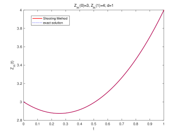
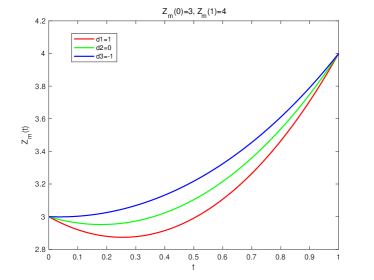
Figure 1: (Color online) (a) The exact solution (dotted line) versus the numerical solution (red line) for (6.9): Initial value z(0) = 3, finial value z(1) = 4, and $d_{\nu_{\alpha,\beta}}=1$, (b) Most probable path for system (6.7) with respect to time interval parameter and $d_{\nu_{\alpha,\beta}}$: Initial value z(0) = 3, finial value z(1) = 4.

Example 2. (A stochastic double-well system)

Consider the following scalar SDE

$$\begin{split}&dX_{t}=(X_{t-}-X_{t-}^{3})dt+dB_{t}+\int_{|x|<1}x\tilde{N}(dt,dx),\\ &f(x)=x-x^{3},\;g(x)=1,\;X_{0}=x_{0}\in\mathbb{R}.\end{split}$$ (6.13)

The deterministic counterpart $\dot{x}=x-x^{3}$ has two stable equilibrium states, -1 and 1, and a unstable equilibrium state, 0. When noise is present, the system (6.13) may show a transition from state -1 to state 1 and then these two states are called metastable states. By means of the theory we have developed in the previous section, we can find the most probable path of the stochastic double-well system (6.13) among all possible smooth curves connecting these two given points.

By Theorem 4.1, the OM function of this system is given by

$$OM(\dot{z},z)=(z-z^{3}-\dot{z})^{2}+1-3z^{2}+2(\dot{z}-z+z^{3})\int_{|\xi|<1}\xi\nu_{\alpha,\beta}(d\xi).$$ (6.14)

And via (5.5)-(5.6), the most probable path $z_{m}(t)$ could be described as the deterministic differential equation:

$$\begin{split}&\ddot{z}_{m}=3z_{m}^{5}-4z_{m}^{3}+3d_{\nu_{\alpha,\beta}}z_{m}^{2}-2z_{m}-d_{\nu_{\alpha,\beta}},\\ &z_{m}(0)=-1,\;\;\;z_{m}(T)=1,\end{split}$$ (6.15)

which can be calculated numerically by the shooting method for the two-point boundary value problem [24]. Note that the OM function given in (6.14) is convex on the variable $\dot{z}$ but the joint mapping $(\dot{z},z)\longmapsto OM(\dot{z},z,)$ is not convex, thus the solution of (6.15) is a local minimizer of functional $\int_{0}^{T}OM(\dot{z},z)dt$ by the Theorem 5.2. We remark that the most probable tube of system (4.1) or, in particular (6.13) depends on the choice of time interval, initial state, final state and the driven $\alpha$-stable noise, more precisely, i.e. constant $d_{\nu_{\alpha,\beta}}$. For $\alpha\in(0,1)$ used for our setting, the value of $d_{\nu_{\alpha,\beta}}=\frac{\alpha}{\Gamma(2-\alpha)\cos(\frac{\pi\alpha}{2})}\beta$ can be positive or negative as $\beta\in[-1,1]$.

Fig 2 shows the most probable paths with initial state -1 and final state 1 of the system (6.13). We choose different values of $T$ to observe the impact of noise on the dynamics. For $T=1$, it is seen that the equation (6.15) describing the most probable path can only be solved when $d_{\nu_{\alpha,\beta}}$ is evaluated in the interval $[-1.9407,1.6305]$. For $T=2$, we obtain an interval $[-1.5150,0.8487]$ for $d_{\nu_{\alpha,\beta}}$. For $T=2.3$, the most probable path of system (6.13) is not available if $d_{\nu_{\alpha,\beta}}$ exceeds the interval $[-1.5057,1.1396]$. Similarly, for $T=6$, $d_{\nu_{\alpha,\beta}}$ is restricted on interval $[-0.8899,0.3836]$. Although $T$ could be any finite value from zero to positive infinity, the corresponding value range of $d_{\nu_{\alpha,\beta}}$ does not always exist as equation (6.15) is not always solvable. It is seen that for different final time $T$, the most probable paths connecting state -1 and state 1 may take different shapes. For every fixed $T$, the most probable paths are also different from each other depending on parameter value $d_{\nu_{\alpha,\beta}}$. In particular, both in Fig 2(a), Fig 2(b), Fig 2(c) and Fig 2(d), the green line that corresponds to $d_{\nu_{\alpha,\beta}}=0$ denotes the most probable path of (6.13) with absence of Lévy noise, (i.e. only driven by Gaussian noise), which is clearly different from those paths with nonzero $d_{\nu_{\alpha,\beta}}$. This finding geometrically displays the effect of non-Gaussian noise on the dynamics.

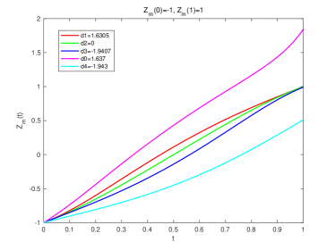
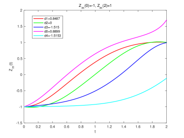
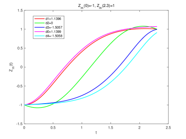
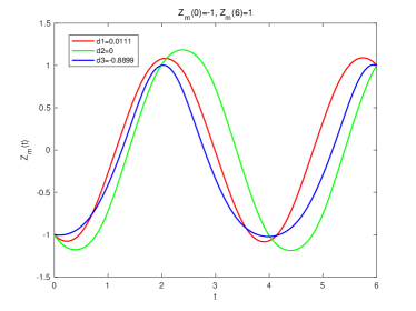
Figure 2: (Color online) Most probable path for system (6.13) with respect to time interval parameter and $d_{\nu_{\alpha,\beta}}$: (a) $T=1$, (b) $T=2$, (c) $T=2.3$, (d) $T=6$.

Note that choices of $\alpha$ and $\beta$ uniquely determine the value of $d_{\nu_{\alpha,\beta}}$. Thus, Fig 3 shows which values of $\alpha$ and $\beta$ correspond to existence (‘green’) or non-existence (‘red’) of the most probable paths from state -1 to state 1 of system (6.13).

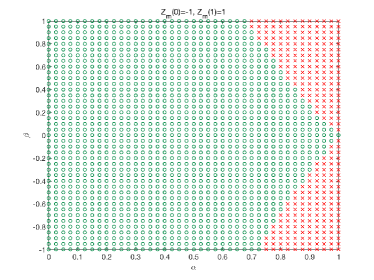
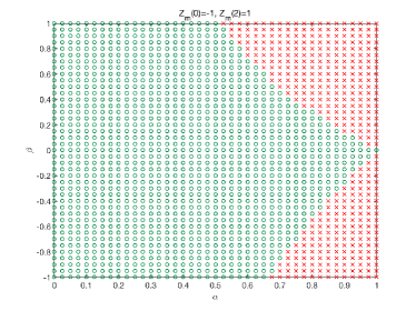
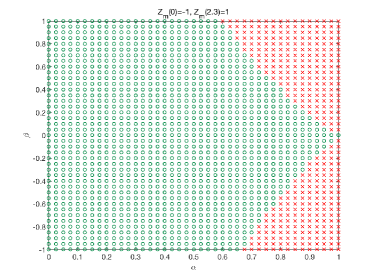
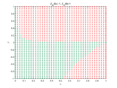
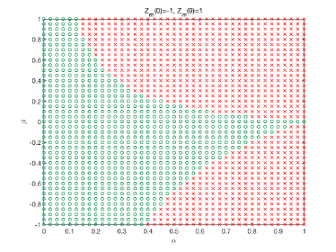
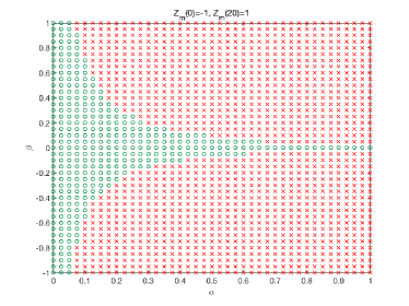
Figure 3: (Color online) The parameter regions of $\alpha$ and $\beta$ with green (red) indicating existence (non-existence) of the most probable paths: (a) $T=1$, (b) $T=2$, (c) $T=2.3$, (d) $T=6$, (e) $T=9$, (f) $T=20$.

7 Conclusion and discussion

In this work, we have derived the Onsager-Machlup function for scalar stochastic differential equations with Lévy motion as well as Brownian motion. With this function as a Lagrangian, we have characterized the most probable path as the solution of the corresponding Euler-Lagrange equation, under two-point boundary conditions. This Onsager-Machlup function is consistent with that for stochastic differential equations with Brownian motion alone, and it thus captures the effect of non-Gaussian fluctuations in understanding the most probable paths.

The most probable paths are often sought, in order to reveal the most likely pathways in transition phenomena [10, 9]. Our work provides a tool to investigate this issue for stochastic dynamical systems with non-Gaussian as well as Gaussian noise, as illustrated in Section 6. Note that this OM theory for the most probable paths does not require noise intensity to be small. Thus it is different from the most probable paths based on large deviation principles, which hold for small noise.

The results of this work (Theorem 4.1) are valid for a scalar stochastic differential equation with a general Lévy process with jump measure $\nu$, as long as the integral $\int_{|\xi|<1}\xi\nu(d\xi)$ is finite. In particular, they are valid for the stochastic differential equations with $\alpha$-stable Lévy motion with $0<\alpha<1$.

Moreover, this work can also be extended to higher dimensional systems (Remark 4.3).

However, this approach to derive Onsager-Machlup action functionals requires non-vanishing and constant diffusion component in the random fluctuations, and appears not to work for stochastic differential equations with pure jump Lévy noise. The Girsanov transformation, which plays a crucial role in this approach, is of little help in pure jump case, since it can not help to obtain the uniqueness in distribution. As also realized earlier in [4] that the Girsanov transformation appears not to work for their case, since it transforms the Poisson process to a general semi-martingale that cannot be handled easily.

Appendix: Proof of (3.1) and (3.2)

We now give the proof of the technical formulas (3.1) and (3.2) which are based on the Itô formula for stochastic integrals.

Proof of (3.1).

By using Itô formula for stochastic integrals, we get

$$dV(Y_{t})= \{\frac{1}{c}a(Y_{t-})k(Y_{t-})+\frac{c}{2}\frac{da(x)}{dx}(Y_{t-})\}dt+a(Y_{t-})dB_{t}$$

$$+\int_{|\xi|<1}[V(Y_{t-}+\xi)-V(Y_{t-})]\tilde{N}(dt,d\xi)+\int_{|\xi|<1}[V(Y_{t-}+\xi)-V(Y_{t-})-\frac{\xi}{c}a(Y_{t-})]\nu(d\xi)dt$$

$$= \{\frac{1}{c}a(Y_{t-})k(Y_{t-})+\frac{c}{2}\frac{da(x)}{dx}(Y_{t-})\}dt+a(Y_{t-})dB_{t}+\int_{|\xi|<1}\frac{\xi}{c}a(Y_{t-})\tilde{N}(dt,d\xi)$$

$$+\int_{|\xi|<1}[V(Y_{t-}+\xi)-V(Y_{t-})-\frac{\xi}{c}a(Y_{t-})]N(dt,d\xi)$$

$$= \{\frac{1}{c}a(Y_{t-})k(Y_{t-})+\frac{c}{2}\frac{da(x)}{dx}(Y_{t-})\}dt+a(Y_{t-})dB_{t}-\int_{|\xi|<1}\frac{\xi}{c}a(Y_{t-})\nu(d\xi)$$

$$+\int_{|\xi|<1}[V(Y_{t-}+\xi)-V(Y_{t-})]N(dt,d\xi).$$

By Integrating from $s$ to $u$ and using the initial condition, we obtain

$$\int_{s}^{u}a(Y_{t-})dB_{t}= V(Y_{u})-V(x_{0})-\frac{1}{2}\int_{s}^{u}\{\frac{2}{c}a(Y_{t-})k(Y_{t-})+c\frac{da(x)}{dx}(Y_{t-})\}dt$$

$$-\int_{s}^{u}\int_{|\xi|<1}[V(Y_{t-}+\xi)-V(Y_{t-})]N(dt,d\xi)+\int_{s}^{u}\int_{|\xi|<1}\frac{\xi}{c}a(Y_{t-})\nu(d\xi)dt$$

$$= V(Y_{u})-V(x_{0})-\frac{1}{2}\int_{s}^{u}\{\frac{2}{c}a(Y_{t-})k(Y_{t-})+c\frac{da(x)}{dx}(Y_{t-})\}dt$$

$$-\Sigma_{s\leq t\leq u}[V(Y_{t})-V(Y_{t-})]\chi_{|\xi|<1}(\Delta Y_{t})+\int_{s}^{u}\int_{|\xi|<1}\frac{\xi}{c}a(Y_{t-})\nu(d\xi)dt,$$

where the last step is based on the definition of Poisson random measure $N(dt,d\xi)$.

Replacing the Ito integral in (3.3) by the relation above, we get the expression $F[y(t)]$ for (3.3) given by (3.1). ∎

Proof of (3.2).

By using Itô formula, we get

$$dV_{X}(X_{t},z_{0}(t))$$

$$= \{\frac{\partial V_{X}(x,z_{0}(t))}{\partial t}\mid_{x=X_{t-}}+\frac{1}{c}a_{X}(X_{t-},z_{0}(t))f(X_{t-})+\frac{c}{2}\frac{\partial a_{X}(x,z_{0}(t))}{\partial t}\mid_{x=X_{t-}}\}dt$$

$$+a_{X}(X_{t-},z_{0})dB_{t}+\int_{|\xi|<1}[V_{X}(X_{t-}+\xi,z_{0}(t))-V_{X}(X_{t-},z_{0}(t))]\tilde{N}(dt,d\xi)$$

$$+\int_{|\xi|<1}[V_{X}(X_{t-}+\xi,z_{0}(t))-V_{X}(X_{t-},z_{0}(t))-\frac{\xi}{c}a_{X}(X_{t-},z_{0}(t))]\nu(d\xi)dt$$

$$= \{\frac{\partial V_{X}(x,z_{0}(t))}{\partial t}\mid_{x=X_{t-}}+\frac{1}{c}a_{X}(X_{t-},z_{0}(t))f(X_{t-})+\frac{c}{2}\frac{\partial a_{X}(x,z_{0}(t))}{\partial t}\mid_{x=X_{t-}}\}dt$$

$$+a_{X}(X_{t-},z_{0})dB_{t}+\int_{|\xi|<1}\frac{\xi}{c}a_{X}(X_{t-},z_{0}(t))\tilde{N}(dt,d\xi)$$

$$+\int_{|\xi|<1}[V_{X}(X_{t-}+\xi,z_{0}(t))-V_{X}(X_{t-},z_{0}(t))-\frac{\xi}{c}a_{X}(X_{t-},z_{0}(t))]N(dt,d\xi)$$

$$= \{\frac{\partial V_{X}(x,z_{0}(t))}{\partial t}\mid_{x=X_{t-}}+\frac{1}{c}a_{X}(X_{t-},z_{0}(t))f(X_{t-})+\frac{c}{2}\frac{\partial a_{X}(x,z_{0}(t))}{\partial t}\mid_{x=X_{t-}}\}dt$$

$$+a_{X}(X_{t-},z_{0})dB_{t}-\int_{|\xi|<1}\frac{\xi}{c}a_{X}(X_{t-},z_{0}(t))\nu(d\xi)dt$$

$$+\int_{|\xi|<1}[V_{X}(X_{t-}+\xi,z_{0}(t))-V_{X}(X_{t-},z_{0}(t))]N(dt,d\xi).$$

By integrating above formula from $s$ to $u$, we obtain:

$$\int_{s}^{u}a_{X}(X_{t-},z_{0})dB_{t}$$

$$= V_{X}(X_{u},z_{0}(u))-V_{X}(x_{0},z_{0}(s))+\int_{s}^{u}\int_{|\xi|<1}\frac{\xi}{c}a_{X}(X_{t-},z_{0})\nu(d\xi)dt$$

$$-\frac{1}{2}\int_{s}^{u}\{2\frac{\partial V_{X}(x,z_{0}(t))}{\partial t}\mid_{x=X_{t-}}+\frac{2}{c}a_{X}(X_{t-},z_{0}(t))f(X_{t-})+c\frac{\partial a_{X}(x,z_{0}(t))}{\partial t}\mid_{x=X_{t-}}\}dt$$

$$-\int_{s}^{u}\int_{|\xi|<1}[V_{X}(X_{t-}+\xi,z_{0}(t))-V_{X}(X_{t-},z_{0}(t))]N(dt,d\xi)$$

$$= V_{X}(X_{u},z_{0}(u))-V_{X}(x_{0},z_{0}(s))+\int_{s}^{u}\int_{|\xi|<1}\frac{\xi}{c}a_{X}(X_{t-},z_{0})\nu(d\xi)dt$$

$$-\frac{1}{2}\int_{s}^{u}\{2\frac{\partial V_{X}(x,z_{0}(t))}{\partial t}\mid_{x=X_{t-}}+\frac{2}{c}a_{X}(X_{t-},z_{0}(t))f(X_{t-})+c\frac{\partial a_{X}(x,z_{0}(t))}{\partial t}\mid_{x=X_{t-}}\}dt$$

$$-\Sigma_{s\leq t\leq u}[V_{X}(X_{t},z_{0}(t))-V_{X}(X_{t-},z_{0}(t))]\chi_{|\xi|<1}(\Delta X_{t}).$$

Replacing the Ito integral in (3.13) by the relation above, we get the expression $J_{X}[X_{t},z_{0}(t)]$ for (3.13) given by (3.2). ∎

References

References

- [1] Applebaum D 2009 Lévy Processes and Stochastic Calculus 2nd ed (New York: Cambridge University Press)
- [2] Albeverio S, Brzezniak Z and WU J 2010 Existence of global solutions and invariant measures for stochastic differential equations driven by poisson type noise with non-lipschitz coefficients Journal of Mathematical Analysis and Applications 371(1) 309-322
- [3] Bach A, Dürr D and Stawicki B 1977 Functionals of Paths of a Diffusion Process and Onsager-Machlup Function Z. Physik B 26 191-193
- [4] Bardina X, Rovira C and Tindel S 2002 Asymptotic evaluation of the poisson measures for tubes around jump curves Applications Mathematicae 29(2) 145-156
- [5] Böttcher B, Schilling R L and Wang J 2014 Lévy Matters III: Lévy-Type Processes: Construction, Approximation and Sample Path Properties (New York: Springer)
- [6] Bröcker J 2018 What is the correct cost functional for variational data assimilation? Climate Dynamics 11 1-11
- [7] Deza R, Izús G G and Wio H S 2009 Fluctuation theorems from non-equilibrium onsager-machlup theory for a brownian particle in a time-dependent harmonic potential Central European Journal of Physics 7(3) 472-478
- [8] Ditlevsen P D 1999 Observation of -stable noise induced millennial climate changes from an ice-core record Geophysical Research Letters 26(10) 1441-1444
- [9] Duan J 2015 An Introduction to Stochastic Dynamics (New York: Cambridge University Press)
- [10] Dürr D and Bach A 1978 The Onsager-Machlup Function as Lagrangian for the Most Probable Path of a Diffusion Process Commun. math. Phys. 60 153-170
- [11] Evans L C 2010 Partial Differential Equations 2nd ed (Providence RI: American Mathematical Society)
- [12] Fujita T and Kotani S 1982 The Onsager-Machlup Function for Diffusion Processes J. Math. Kyoto Univ. 22(1) 115-130
- [13] Haas K R, Yang H and Chu J W 2014 Analysis of trajectory entropy for continuous stochastic processes at equilibrium Journal of Physical Chemistry B 118(28) 8099-107
- [14] Hara K and Takahashi Y 2016 Stochastic analysis in a tubular neighborhood or onsager-machlup functions revisited arXiv:1610.06670v1
- [15] Hartman P 2002 Ordinary Differential Equations 2nd ed (Philadephia: Society for industrial and applied mathematics)
- [16] Kuo H H 1975 Gaussian measures in Banach spaces in: Lecture notes in mathematics 463 (Berlin-Heidelberg-New York: Springer)
- [17] Ishikawa Y 2013 Stochastic Calculus of Variations for Jump Processes (Berlin: Walter de Gruyter)
- [18] Ikeda N and Watanabe S 1989 Stochastic Differential Equations and Diffusion Processes 2nd ed (Amsterdam: North-Holland Mathcmnticnl Library)
- [19] Moret S and Nualart D 2002 Onsager-Machlup functional for the fractional Brownian motion Probab. Theory. Rel. 124(2) 227-260
- [20] Oksendal B 2003 Stochastic Differential Equations 6th ed (Berlin: Springer)
- [21] Onsager L and Machlup S 1953 Fluctuations and irreversible processes, I, II Phys. Rev. 91 1505-1512 1512-1515
- [22] Pollard D 1984 Convergence of Stochastic Processes (New York: Springer)
- [23] Sato K-I 1999 Lévy Processes and Infinitely Divisible Distributions (Cambridge: Cambridge University Press)
- [24] Sebestyen G 2011 Numerical Solution of Two point Boundary Value Problems B.S.C Theses Department of Applied Analysis Lorand University Budapest
- [25] Singh N 2008 Onsager-machlup theory and work fluctuation theorem for a harmonically driven brownian particle Journal of Statistical Physics 131(3) 405-414
- [26] Stratonovich R L 1971 On the Probability Functional of Diffusion Processes Selected Trans. in Math. Stat. Prob 10 273-286
- [27] Sugiura N 2017 The onsager–machlup functional for data assimilation Nonlinear Processes in Geophysics 24(4) 1-15
- [28] Tisza L and Manning I 1957 Fluctuations and Irreversible Thermodynamics Phys. Rev. 105(6) 1695-1705
- [29] Takahashi Y and Watanabe S 1980 The Probability Functionals (Onsager- Machlup Functions) of Diffusion Processes Springer Lecture Notes in Math. 851 432-463
- [30] Wan X, Yu H and Zhai J 2018 Convergence analysis of a finite element approximation of minimum action methods Siam J. Numer. Anal. 56(3) 1597-1620
- [31] Woyczyński W 2001 Lévy processes in the physical sciences Lévy processes: Theory and Applications (Boston: Birkhäuser)
- [32] Wang H, Cheng X, Daun J, Kurths and Li X 2018 Likelihood for transcriptions in a genetic regulatory system under asymmetric stable Lévy noise Chaos 28 013121
- [33] Xi F and Zhu C 2017 Jump type stochastic differential equations with non-Lipschitz coefficients: Non-confluence, Feller and strong Feller properties, and exponential ergodicity J. Differential Equations revised
- [34] Zheng Y, Serdukova L, Duan J and Kurths J 2016 Transitions in a genetic transcriptional regula- tory system under Lévy motion Sci. Rep. 6 29274