Topological classification of the single-wall carbon nanotube

Abstract

The single-wall carbon nanotube (SWNT) can be a one-dimensional topological insulator, which is characterized by a $\mathbb{Z}$-topological invariant, winding number. Using the analytical expression for the winding number, we classify the topology for all possible chiralities of SWNTs in the absence and presence of a magnetic field, which belongs to the topological categories of BDI and AIII, respectively. We find that the majority of SWNTs are nontrivial topological insulators in the absence of a magnetic field. In addition, the topological phase transition takes place when the band gap is closed by applying a magnetic field along the tube axis, in all the SWNTs except armchair nanotubes. The winding number determines the number of edge states localized at the tube ends by the bulk-edge correspondence, the proof of which is given for SWNTs in general. This enables the identification of the topology in experiments.

I Introduction

The single-wall carbon nanotube (SWNT) is a quasi-one-dimensional (1D) material made by rolling up a graphene sheet, which possesses two Dirac cones at $K$ and $K^{\prime}$ points. The circumference of nanotube is represented by the chiral vector, $\bm{C}_{\rm h}=n\bm{a}_{1}+m\bm{a}_{2}$, on the graphene, where $\bm{a}_{1}$ and $\bm{a}_{2}$ are the primitive lattice vectors and a set of two integers, $(n,m)$, is called chirality Saito1998 . The SWNT is metallic (semiconducting) for ${\rm mod}(2n+m,3)=0$ $(\neq 0)$, because some wavevectors discretized in the circumference direction pass (do not pass) through $K$ or $K^{\prime}$ points when they are expressed in the two-dimensional (2D) Brillouin zone (BZ) of graphene. Even for metallic SWNTs, a narrow band gap opens due to the finite curvature in the tube surface Hamada1992 ; Saito1992 ; Kane1997 . The curvature enhances the spin-orbit (SO) interaction through the mixing between $\pi$ and $\sigma$ orbitals, which also contributes to the band gap Ando2000 .

Recently, SWNTs have attracted attention from a viewpoint of topology Klinovaja2012 ; Egger2012 ; Sau2013 ; Hsu2015 ; Izumida2016 ; Lin2016 ; Okuyama2017 ; Izumida2017 ; Marganska2018 ; Zang2018 . The neutral SWNT can be regarded as a 1D insulator in the presence of band gap and rotational symmetry (see below). Due to the sublattice (or chiral) symmetry between $A$ and $B$ lattice sites, the topology of a SWNT is characterized by a $\mathbb{Z}$ topological invariant, winding number Wen1989 . SWNTs can be 1D topological insulators in both the absence and presence of a magnetic field, which belong to classes BDI and AIII in the periodic table in Ref. Schnyder2009 , respectively. Izumida et al. introduced the winding number for semiconducting SWNTs for the first time Izumida2016 . They also examined the edge states localized around the tube ends with energy $E=E_{\rm F}=0$, the number of which is related to the winding number by the bulk-edge correspondence. This enables us to know the winding number via the observation of local density of states at the tube ends by the scanning tunneling microscopy as already done for the graphene Kobayashi2005 . The present authors generalized the theory for metallic SWNTs Okuyama2017 . The narrow band gap in metallic SWNTs can be closed by applying a magnetic field of a few Tesla along the tube axis. This results in the topological phase transition, where the winding number changes discontinuously as a function of the magnetic field. Independently, Lin et al. examined the topological nature in a zigzag SWNT ($n>0$ and $m=0$) by using the Su-Schrieffer-Heeger model and topological invariant called Zak phase Lin2016 . They theoretically proposed a possible manipulation of the edge states via the topological phase transition, although it requires an unrealistically huge magnetic field in the case of a semiconducting SWNT. There also exist theoretical studies on topological phases in a SWNT proximity coupled to a superconductor Klinovaja2012 ; Egger2012 ; Sau2013 ; Hsu2015 ; Izumida2017 ; Marganska2018 .

In the present study, we topologically classify all possible SWNTs. The winding number is analytically derived for all possible chiralities. We also generalize the bulk-edge correspondence to the cases of both semiconducting and metallic SWNTs in a magnetic field along the tube axis, which determines the number of edge states by the winding number. Our main results are depicted in Fig. 3: (a) In the absence of a magnetic field, the majority of SWNTs are topological insulators with nonzero winding number. The exceptions are metallic SWNTs of armchair type ($n=m$) and semiconducting SWNTs with $n=m+1$. (b) In the presence of a magnetic field, the topological phase transition takes place when the band gap is closed by applying a magnetic field, for all SWNTs other than the armchairs. In other words, the SWNT can be topologically nontrivial even for $n=m+1$ when the magnetic field is tuned appropriately. Only armchair nanotubes are topologically trivial regardless of the magnetic field, which is due to the mirror symmetry with respect to a plane including the tube axis Izumida2016 . Previously, some groups theoretically predicted a change in the number of edge states in a SWNT as a function of magnetic field Sasaki2005 ; Sasaki2008 ; Marganska2011 . Our theory clearly explains their physical origin in terms of topology.

We noticed a theoretical study by Zang et al. Zang2018 during the preparation of this paper. They utilized a similar technique to ours to analyze the winding number in SWNTs. They showed that some SWNTs can have the edge states and that the topological phase transition takes place by applying a magnetic field. Their study, however, was only applicable to semiconducting SWNTs, and they did not derive analytic expression for the winding number.

This paper is organized as follows. In Sec. II, we introduce a 1D lattice model for semiconducting SWNTs in the absence of a magnetic field, utilizing the rotational symmetry. We include a magnetic field along the tube axis in Sec. III. In Sec. IV, we analytically evaluate the winding numbers in the case of semiconducting SWNTs in both the absence and presence of a magnetic field. The winding number determines the number of edge states via the bulk-edge correspondence, whose proof is given in Appendix B. In Sec. V, we examine the topology in metallic SWNTs with small band gap induced by the curvature effects. After the discussion on our theoretical study in Sec. VI, our conclusions are given in Sec. VII.

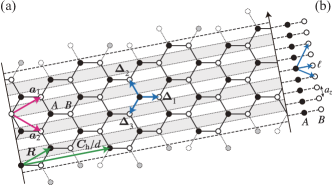
Figure 1: (Color online) (a) The mapping of the $(n,m)$-SWNT to a graphene sheet. The chiral vector, $\bm{C}_{\rm h}=n\bm{a}_{1}+m\bm{a}_{2}$, indicates the circumference of the tube with $\bm{a}_{1}$ and $\bm{a}_{2}$ being the primitive lattice vectors of graphene. The three vectors $\bm{\Delta}_{j}$ $(j=1,2,3)$ connect the nearest-neighbor atoms. The $d$-fold symmetry around the tube axis (helical symmetry) corresponds to the translational symmetry of $\bm{C}_{\rm h}/d$ $(\bm{R}=p\bm{a}_{1}+q\bm{a}_{2})$, where $d=\gcd(n,m)$ and integers $p$ and $q$ are given by Eq. (3). This figure shows the case of $(n,m)=(6,3)$ with $d=3$, $p=1$, and $q=0$. (b) A 1D lattice model in which $A$ and $B$ lattice sites are aligned in the axial direction.

II 1D lattice model for semiconducting nanotube

In this section, we derive a 1D lattice model for semiconducting SWNTs in the absence of a magnetic field. Neither the Aharonov-Bohm (AB) effect in a magnetic field nor curvature-induced narrow gap in metallic SWNTs are considered.

Throughout the paper, we consider the $(n,m)$-SWNT, whose circumference is specified by chiral vector $\bm{C}_{\rm h}=n\bm{a}_{1}+m\bm{a}_{2}$ on a graphene sheet, where $\bm{a}_{1/2}=(\sqrt{3}/2,\pm 1/2)a$ with the lattice constant $a=0.246~{}{\rm nm}$ [see Fig. 1(a)]. Its diameter is given by $d_{\rm t}=|\bm{C}_{\rm h}|/\pi=a\sqrt{n^{2}+nm+m^{2}}/\pi$. The chiral angle $\theta$ is defined as the angle between $\bm{C}_{\rm h}$ and $\bm{a}_{1}$: $\theta=\tan^{-1}[\sqrt{3}m/(2n+m)]$. We restrict ourselves to the case of $0\leq m\leq n$ without loss of generality, which corresponds to $0\leq\theta\leq\pi/6$ with $\theta=0$ and $\pi/6$ for zigzag ($m=0$) and armchair ($m=n$) nanotubes, respectively.

II.1 Derivation

We start from the tight-binding model for graphene Saito1998 , which consists of $A$ and $B$ sublattices, as depicted by filled and empty circles, respectively, in Fig. 1(a). This model involves an isotropic hopping integral $\gamma$ between the nearest-neighbor atoms. An $A$ atom is connected to three $B$ atoms by vectors $\bm{\Delta}_{j}$ $(j=1,2,3)$ in Fig. 1(a). The Hamiltonian reads

$$H=\sum_{\bm{r}_{A}}\sum_{j=1}^{3}\left(\gamma c^{\dagger}_{\bm{r}_{A}}c_{\bm{r}_{A}+\bm{\Delta}_{j}}+{\rm H.c.}\right),$$ (1)

where $\bm{r}_{\sigma}$ is the position of $\sigma=A$ or $B$ atom on the graphene sheet, and $c_{\bm{r}}$ is the field operator for a $\pi$ electron of atom at position $\bm{r}$. $\gamma=-2\hbar v_{\rm F}/(\sqrt{3}a)$ with $v_{\rm F}=8.32\times 10^{5}~{}{\rm m/s}$ being the Fermi velocity in the graphene. The spin index $s$ is omitted, which is irrelevant in Secs. II and III.

We derive a 1D lattice model of the SWNT along the lines of Ref. Izumida2016 , where the helical-angular construction White1993 ; Jishi1993 is utilized. $(n,m)$-SWNT has the $d$-fold rotational symmetry around the tube axis, where

$$d=\gcd(n,m)$$ (2)

is the greatest common divisor of $n$ and $m$. The rotation by $2\pi/d$ corresponds to the translation by $\bm{C}_{\rm h}/d$ on the graphene sheet. The SWNT also has the helical symmetry represented by the translation by $\bm{R}=p\bm{a}_{1}+q\bm{a}_{2}$ on the graphene sheet, with integers $p$ and $q$ satisfying

$$mp-nq=d.$$ (3)

This means that the SWNT is invariant under the translation by $a_{z}=\sqrt{3}da^{2}/(2\pi d_{\rm t})$ along the tube axis together with the rotation by $\theta_{z}=2\pi[(2n+m)p+(n+2m)q]/[2(n^{2}+nm+m^{2})]$ around it [see Fig. 1(a)]. Here, $\bm{R}$ and $\bm{C}_{\rm h}/d$ are a new set of primitive lattice vectors of graphene; the position of $A$ and $B$ atoms can be expressed as

$$\bm{r}_{A} =\ell\bm{R}+\nu(\bm{C}_{\rm h}/d),$$ (4)

$$\bm{r}_{B} =\ell\bm{R}+\nu(\bm{C}_{\rm h}/d)+\bm{\Delta}_{1},$$ (5)

on the graphene sheet with site indices $\ell$ and $\nu=0,1,2,\ldots,d-1$. By performing the Fourier transformation for the $\nu$ coordinate, we obtain the Hamiltonian block diagonalized in the subspace of orbital angular momentum $\mu=0,1,2,\ldots,d-1$ as $H=\sum_{\mu=0}^{d-1}H_{\mu}$,

$$H_{\mu}=\sum_{\ell}\sum_{j=1}^{3}\left(\gamma{\rm e}^{{\rm i}2\pi\mu\Delta^{\prime\prime}_{j}/d}c^{\,\mu\,\dagger}_{A,\ell}c^{\,\mu}_{B,\ell+\Delta^{\prime}_{j}}+{\rm H.c.}\right).$$ (6)

This is a 1D lattice model in which $A$ and $B$ lattice sites are aligned in the axial direction with the lattice constant $a_{z}$, as shown in Fig. 1(b). Here, $c^{\,\mu}_{\sigma,\ell}$ is the field operator of an electron with angular momentum $\mu$ and at sublattice $\sigma$ of site index $\ell$. The hopping to the $j$th nearest-neighbor atom [vector in $\bm{\Delta}_{j}$ in Fig. 1(a)] gives rise to the hopping to the sites separated by $\Delta^{\prime}_{j}$ in Fig. 1(b) with phase factor $\Delta^{\prime\prime}_{j}$, where

$$\bm{\Delta}_{j}-\bm{\Delta}_{1}=\Delta^{\prime}_{j}\bm{R}+\Delta^{\prime\prime}_{j}(\bm{C}_{\rm h}/d),$$ (7)

or $\Delta^{\prime}_{1}=\Delta^{\prime\prime}_{1}=0$, $\Delta^{\prime}_{2}=n/d$, $\Delta^{\prime\prime}_{2}=-p$, $\Delta^{\prime}_{3}=-m/d$, and $\Delta^{\prime\prime}_{3}=q$.

II.2 Bulk properties

For the bulk system, the Fourier transformation of $H_{\mu}$ along $\ell$ direction yields the two-by-two Hamiltonian,

$$H_{\mu}(k) =\gamma\begin{bmatrix}0&f_{\mu}(k)\\ f^{*}_{\mu}(k)&0\end{bmatrix},$$ (8)

in the sublattice space for given wave number $k$. $k$ runs through the 1D BZ, $-\pi\leq ka_{z}<\pi$, and

$$f_{\mu}(k) =\sum_{j=1}^{3}{\rm e}^{{\rm i}2\pi\mu\Delta^{\prime\prime}_{j}/d}{\rm e}^{{\rm i}ka_{z}\Delta^{\prime}_{j}}.$$ (9)

The dispersion relation for subband $\mu$ is readily obtained as

$$E_{\mu}(k) =\pm|\gamma f_{\mu}(k)|.$$ (10)

The system is an insulator for semiconducting SWNTs with ${\rm mod}(2n+m,3)\neq 0$, that is, $f_{\mu}(k)\neq 0$ in the whole BZ. Then, the positive and negative $E_{\mu}(k)$’s form the conduction and valence bands, respectively. On the other hand, for metallic SWNTs with ${\rm mod}(2n+m,3)=0$, $f_{\mu}(k)$ becomes zero at $\mu_{+}$ and $k_{+}$ ($\mu_{-}$ and $k_{-}$) that correspond to the $K$ ($K^{\prime}$) point on the graphene sheet, as discussed in Sec. V.

II.3 Winding number and bulk-edge correspondence

The bulk Hamiltonian in Eq. (8) anticommutes with $\sigma_{z}$ in the sublattice space, which is called sublattice or chiral symmetry. Thanks to this symmetry as well as the finite band gap, we can define the winding number Wen1989 ,

$$w_{\mu}=\int_{-\pi/a_{z}}^{\pi/a_{z}}\frac{{\rm d}k}{2\pi}\frac{\partial}{\partial k}\arg f_{\mu}(k)\equiv\frac{1}{2\pi}\oint_{\rm BZ}{\rm d}\arg f_{\mu}(k),$$ (11)

for subband with angular momentum $\mu$ in semiconducting SWNTs Izumida2016 . The winding number is the number of times that $f_{\mu}(k)$ in Eq. (9) winds around the origin on the complex plane when $k$ runs through the 1D BZ. Note that $w_{\mu}$ in Eq. (11) is ill-defined for metallic SWNTs where $f_{\mu}(k)$ is zero and therefore $\arg f_{\mu}(k)$ cannot be defined at $\mu_{\tau}$ and $k_{\tau}$ ($\tau=\pm 1$). We will overcome this problem in Sec. V.

The bulk-edge correspondence holds between the winding number and number of edge states, $N_{\rm edge}$,

$$N_{\rm edge}=4\sum_{\mu=0}^{d-1}|w_{\mu}|$$ (12)

in a long but finite SWNT. The prefactor of 4 is ascribable to the spin degeneracy and two edges at tube ends. This relation was analytically shown for semiconducting SWNTs in the absence of a magnetic field in Ref. Izumida2016 . We generalize Eq. (12) [and Eq. (29)] for both semiconducting and metallic SWNTs in a magnetic field in Appendix B. Here, we assume that the tube is cut by a broken line in Fig. 1(a), which results in so-called minimal boundary edges Akhmerov2008 . The case of the other boundaries is discussed in Sec. VI.

III 1D lattice model with finite magnetic field

We extend our theory to include a magnetic field $B$ in the axial direction of the SWNT. We neglect the spin-Zeeman effect throughout the paper, which is justified unless the band gap is closed in a huge magnetic field. Only the AB effect is taken into account as the Peierls phase in the hopping integral. We replace

$$\gamma{\rm e}^{{\rm i}2\pi\mu\Delta^{\prime\prime}_{j}}\rightarrow\gamma{\rm e}^{{\rm i}2\pi\mu\Delta^{\prime\prime}_{j}}\exp\left({\rm i}2\pi\phi\frac{a_{\rm CC}\cos\Theta_{j}}{\pi d_{\rm t}}\right)$$ (13)

in $H_{\mu}$ in Eq. (6) and $H_{\mu}(k)$ in Eq. (8). Here,

$$\phi=\frac{B\,\pi(d_{\rm t}/2)^{2}}{h/e}$$ (14)

is the AB phase, or number of flux quanta penetrating the tube, $a_{\rm CC}=a/\sqrt{3}$ is the bond length $|\bm{\Delta}_{j}|$, and $\Theta_{j}$ is the angle between $\bm{\Delta}_{j}$ and $\bm{C}_{\rm h}$ on the graphene sheet: $\Theta_{j}=\theta-(5\pi/6)+(2\pi/3)j$.

As a result, $f_{\mu}(k)$ in Eq. (9) changes to

$$f_{\mu}(k;\phi) =\sum_{j=1}^{3}{\rm e}^{{\rm i}2\pi\mu\Delta^{\prime\prime}_{j}/d}\exp\left({\rm i}2\pi\phi\frac{a_{\rm CC}\cos\Theta_{j}}{\pi d_{\rm t}}\right){\rm e}^{{\rm i}ka_{z}\Delta^{\prime}_{j}}$$ (15)

in a magnetic field. $f_{\mu}(k;\phi)$ can be zero even for semiconducting SWNTs, that is, the band gap is closed at $|\phi|=\phi^{*}=1/3$ Ajiki1993 . When $|\phi|\neq\phi^{*}$, $w_{\mu}$ in Eq. (11) can be defined in terms of $f_{\mu}(k;\phi)$. As we will show later, a sudden change in $w_{\mu}$ takes place at $|\phi|=\phi^{*}=1/3$, which corresponds to the topological phase transition.

Note that only the decimal part of $\phi$ is physically significant. $\phi\rightarrow\phi+1$ compensates with $\mu\rightarrow\mu-1$ in the definition of angular momentum. Therefore, we can restrict ourselves to $0\leq\phi<1$ or $-1/2\leq\phi<1/2$, depending on the situations.

IV Topological classification of semiconducting nanotube

Now we topologically classify semiconducting SWNTs. The winding number $w_{\mu}$ is analytically evaluated as a function of chirality $(n,m)$ and magnetic field $B$ in the axial direction. The winding number $w_{\mu}$ in Eq. (11) can be interpreted as the number of times that $f_{\mu}(k)$ or $f_{\mu}(k;\phi)$ circulates around the origin on the complex plane when $k$ runs through the 1D BZ, $-\pi\leq ka_{z}<\pi$.

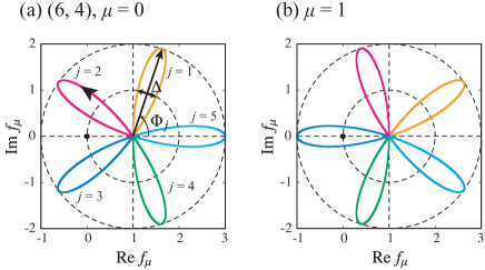
Figure 2: (Color online) $f_{\mu}(k)$ on the complex plane for the (6, 4)-SWNT with (a) $\mu=0$ and (b) $\mu=1$. $d=2$ and we choose $p=q=-1$. It draws a flower-shaped trajectory centered at $z=1$, with petal $j=1$ to $5$. The distance from $z=1$ takes its maximum, $2$, when the argument measured from $z=1$ is $\Phi_{j}$ in Eq. (17), whereas it is 1 for $\Phi_{j}\pm\Delta/2$.

IV.1 Analysis without magnetic field

We begin with the case in the absence of a magnetic field (AB phase $\phi=0$). From Eq. (9), we obtain

$$f_{\mu}(k)=1+2 \cos\left[\frac{n+m}{2d}ka_{z}-\frac{\pi\mu}{d}(p+q)\right]$$

$$\times \exp\left\{{\rm i}\left[\frac{n-m}{2d}ka_{z}+\frac{\pi\mu}{d}(-p+q)\right]\right\}.$$ (16)

For armchair SWNTs of $n=m$ [$d=n$ in Eq. (2) and $p=1$ and $q=0$ in Eq. (3)], Eq. (16) indicates a line segment on the complex plane. For SWNTs other than armchair type, $f_{\mu}(k)$ draws a “flower-shaped” closed loop, as depicted for the $(6,4)$-SWNT with $\mu=0$ and $1$ in Figs. 2(a) and 2(b), respectively. We can see that the former does not circulate the origin, whereas the latter does. This results in $w_{\mu=0}=0$ and $w_{\mu=1}=1$, respectively. In general, the trajectory is centered at $z=1$, and $|f_{\mu}(k)-1|$ takes the maximum value, $2$, when

$$\arg\left[f_{\mu}(k)-1\right]=\frac{2\pi d}{n+m}\left(j-\frac{\mu}{d}\right)\equiv\Phi_{j},$$ (17)

with $j=1,2,\dots,\frac{n+m}{d}$. Note that $0<\Phi_{j}\leq 2\pi$ for $0\leq\mu<d$. $|f_{\mu}(k)-1|=1$ when $\arg[f_{\mu}(k)-1]=\Phi_{j}\pm\Delta/2$ with $\Delta=\frac{2\pi}{3}(n-m)/(n+m)$. Therefore, the $j$th “petal” surrounds the origin when $\Phi_{j}-\Delta/2<\pi<\Phi_{j}+\Delta/2$, that is,

$$\frac{n+2m}{3d}+\frac{\mu}{d}<j<\frac{2n+m}{3d}+\frac{\mu}{d}.$$ (18)

$w_{\mu}$ is equal to the number of integers $j$ that satisfy Eq. (18) for given $(n,m)$ and $\mu$. We evaluate $w_{\mu}$ for semiconducting SWNTs [${\rm mod}(2n+m,3)\neq 0$] in Table 1, which are categorized according to ${\rm mod}(\frac{2n+m}{d},3)=1$ or $2$. The table also includes $w_{\mu}$ for metallic SWNTs with ${\rm mod}(2n+m,3)=0$ when the number of times that $f_{\mu}(k)$ passes the origin is neglected.

Table 1: The winding number $w_{\mu}$ determined by the number of times that $f_{\mu}(k)$ winds around the origin on the complex plane when $k$ runs through the 1D BZ. We assume $0\leq m\leq n$, and $d=\gcd(n,m)$. $\mu$ is an integer (angular momentum) in the absence of a magnetic field while it is a real number in the presence of an axial magnetic field (see text in Sec. IV B). For metallic SWNTs, we disregard the number of times that $f_{\mu}(k)$ passes the origin.

Type	$w_{\mu}$
${\rm mod}\left(\frac{2n+m}{d},3\right)=1$ (semiconductor or metal-1)
	$\begin{cases}\frac{(n-m)/d-2}{3}&\left(\frac{d}{3}\leq\mu\leq\frac{2d}{3}\right)\\ \frac{(n-m)/d+1}{3}&\left(0\leq\mu<\frac{d}{3}~{}{\rm or}~{}\frac{2d}{3}<\mu<d\right)\end{cases}$
${\rm mod}\left(\frac{2n+m}{d},3\right)=2$ (semiconductor or metal-1)
	$\begin{cases}\frac{(n-m)/d+2}{3}&\left(\frac{d}{3}<\mu<\frac{2d}{3}\right)\\ \frac{(n-m)/d-1}{3}&\left(0\leq\mu\leq\frac{d}{3}~{}{\rm or}~{}\frac{2d}{3}\leq\mu<d\right)\end{cases}$
${\rm mod}\left(\frac{2n+m}{d},3\right)=0$ and $n\neq m$ (metal-2 other than armchair)
	$\begin{cases}\frac{n-m}{3d}-1&(\mu=0)\\ \frac{n-m}{3d}&(0<\mu<d)\end{cases}$
$n=m$ (metal-2 of armchair type)
	$0\qquad(0\leq\mu<d)$

IV.2 Analysis with finite magnetic field

When the axial magnetic field is present, the trajectory of $f_{\mu}(k;\phi)$ is examined to evaluate $w_{\mu}$. We obtain $\Phi_{j}$ in Eq. (17) with $\mu$ replaced by $\mu+\phi$, which means that the trajectory for each $\mu$ is rotated around $z=1$ on the complex plane Zang2018 . As we mentioned earlier in Sec. III, only the decimal part of $\phi$ is physically meaningful because $\phi\rightarrow\phi^{\prime}=\phi-\lfloor\phi\rfloor$ is equivalent to $\mu\rightarrow\mu^{\prime}=\mu+\lfloor\phi\rfloor$ with $\lfloor x\rfloor$ being the maximum integer not exceeding $x$. Thus we can make the same analysis as in the previous subsection with $\mu^{\prime}=0,1,2,\ldots,d-1$, $0\leq\phi^{\prime}<1$, and $0<\Phi_{j}\leq 2\pi$. Then the replacement of $\mu$ by $\mu^{\prime}+\phi^{\prime}$ yields the same result as in Table 1.

IV.3 Edge states and topological order

By summing up $w_{\mu}$ in Eq. (12) carefully, we obtain the number of edge states $N_{\rm edge}$, as shown in Table 2. Here, we assume $-1/2\leq\phi<1/2$ ($\mu$ should be shifted accordingly). The semiconducting SWNTs are categorized into type-1 and type-2 for ${\rm mod}(2n+m,3)=1$ or $2$. The results for $N_{\rm edge}$ indicate that (i) the semiconducting SWNTs other than $n=m+1$ are topological nontrivial in the absence of a magnetic field (AB phase $\phi=0$) and (ii) all the semiconducting SWNTs show the topological phase transition at $|\phi|=\phi^{*}=1/3$ when the energy gap is closed Ajiki1993 . Note that $|\phi|=1/3$ corresponds to the magnetic field of more than $100~{}{\rm T}$ when the tube diameter $d_{\rm t}\sim 1~{}{\rm nm}$. Table 2 also includes the results for metallic SWNTs, that are topological insulators except for the armchair nanotubes, irrespectively of the magnetic field, as discussed in the next section.

Figure 3(a) illustrates the number of edge states at $B=0$, where a hexagon from the leftmost one indicates the chiral vector $\bm{C}_{\rm h}=n\bm{a}_{1}+m\bm{a}_{2}$. Almost all the SWNTs have edge states except for the semiconducting SWNTs with $n=m+1$ and metallic ones of armchair type. Figure 3(b) shows the critical magnetic field for the topological phase transition, where the number of edge states changes discontinuously. The critical magnetic field should be experimentally accessible for metallic SWNTs with $d_{\rm t}\gtrsim 1~{}{\rm nm}$ (see Sec. V).

Table 2: Number of edge states $N_{\rm edge}$ in the $(n,m)$-SWNT. We assume $0\leq m\leq n$. The number of flux quanta $\phi$ is restricted to $-1/2\leq\phi<1/2$. $\Theta(x)=1$ ($0$) for $x>0$ ($x<0$).

Type	Number of edge states $N_{\rm edge}$
Semiconductor type-1 [${\rm mod}(2n+m,3)=1$]
	$\begin{cases}4\frac{n-m+1}{3}&(0\leq|\phi|<\frac{1}{3})\\ 4\frac{n-m-2}{3}&(\frac{1}{3}<|\phi|\leq\frac{1}{2})\\ \end{cases}$
Semiconductor type-2 [${\rm mod}(2n+m,3)=2$]
	$\begin{cases}4\frac{n-m-1}{3}&(0\leq|\phi|<\frac{1}{3})\\ 4\frac{n-m+2}{3}&(\frac{1}{3}<|\phi|\leq\frac{1}{2})\\ \end{cases}$
Metal other than armchair [${\rm mod}(2n+m,3)=0$ and $n\neq m$]
	$4\left(\frac{n-m}{3}-1\right)+2\sum_{\tau,s}\Theta(\Delta k_{c}+\tau s\Delta k_{\rm so}+\tau\Delta k_{\phi})$
Metal of armchair type ($n=m$)
	0

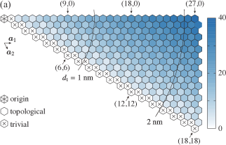
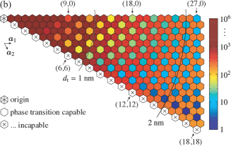
Figure 3: (Color online) (a) Number of edge states in the absence of a magnetic field ($B=0$) and (b) critical magnetic field $B^{*}$ of topological phase transition at which the number of edge states changes discontinuously. A hexagon from the leftmost one indicates the chiral vector $\bm{C}_{\rm h}=n\bm{a}_{1}+m\bm{a}_{2}$, where $\bm{a}_{1}$ and $\bm{a}_{2}$ are the primitive lattice vectors of graphene, shown in Fig. 1.

The number of edge states per diameter approaches $N_{\rm edge}/d_{\rm t}\rightarrow 4(n-m)/(3d_{\rm t})$ as $d_{\rm t}$ increases. This agrees with the result in Ref. Akhmerov2008 for the edge states of graphene. We thus obtain an asymptotic form of $N_{\rm edge}$ for large $d_{\rm t}$,

$$N_{\rm edge}\simeq\frac{8\pi d_{\rm t}}{3a}\cos\left(\theta+\frac{\pi}{3}\right).$$ (19)

This should be useful when a nanotube of large diameter is examined in a continuum approximation.

V Analysis for metallic nanotube

In this section, we discuss the topology of metallic SWNTs with ${\rm mod}(2n+m,3)=0.$ Without the curvature-induced effects, a band of angular momentum $\mu_{+}$ ($\mu_{-}$) passes the Dirac point $K$ ($K^{\prime}$) with wave number $k_{+}$ ($k_{-}$) on the graphene sheet:

$$\mu_{\pm} =\pm\frac{2n+m}{3}=\pm\frac{d}{3}{\rm mod}\left(\frac{2n+m}{d},3\right)\quad({\rm mod}~{}d),$$ (20)

$$k_{\pm} =\pm\frac{2\pi}{3a_{z}}(2p+q),$$ (21)

Izumida2016 . Metallic SWNTs are classified into metal-1 for ${\rm mod}(\frac{2n+m}{d},3)\neq 0$ and metal-2 for ${\rm mod}(\frac{2n+m}{d},3)=0$. $\mu_{+}\neq\mu_{-}~{}({\rm mod}~{}d)$ in the former, whereas $\mu_{+}=\mu_{-}=0$ in the latter.

In order to describe the narrow energy gap in metallic SWNTs, we further extend our 1D lattice model to include the curvature-induced effects besides the AB effect in a magnetic field. As seen in Appendix A, our model is constructed so as to reproduce the effective Hamiltonian for $\bm{k}\cdot\bm{p}$ theory, which describes the curvature-induced effects and SO interaction Izumida2009 , in the vicinity of $k_{\pm}$ with angular momentum $\mu_{\pm}$.

V.1 1D lattice model with curvature effects

The effective Hamiltonian for $\bm{k}\cdot\bm{p}$ theory is given by

$$H= \sum_{\bm{r}_{A},s}\sum_{j=1}^{3}\left(\gamma^{(1)}_{s,j}\,c^{\,s\,\dagger}_{\bm{r}_{A}}c^{\,s}_{\bm{r}_{A}+\bm{\Delta}_{j}}+{\rm H.c.}\right)$$

$$+ \sum_{\sigma=A,B}\sum_{\bm{r}_{\sigma},s}\sum_{j=1}^{6}\gamma^{(2)}_{s,j}\,c^{\,s\,\dagger}_{\bm{r}_{\sigma}}c^{\,s}_{\bm{r}_{\sigma}+\bm{\Delta}^{\!\!(2)}_{j}}$$ (22)

with $c^{\,s}_{\bm{r}}$ being the field operator for a $\pi$ electron with spin $s$ at atom of position $\bm{r}$ Okuyama2017 . The quantization axis for spin $s=\pm 1$ is chosen in the tube direction Izumida2009 . This model consists of anisotropic and spin-dependent hopping integrals to the nearest-neighbor atoms and those to the second nearest neighbors. As mentioned in Sec. II B, the former connects $A$ and $B$ atoms that are depicted by three vectors $\bm{\Delta}_{j}$ $(j=1,2,3)$, whereas the latter connects atoms of the same species indicated by six vectors $\bm{\Delta}^{\!\!(2)}_{j}$ $(j=1,2,\ldots,6)$ in Fig. 4(a). The explicit forms of hopping integrals, $\gamma^{(i)}_{s,j}$ $(i=1,2)$, are provided in Appendix A.

As described in Sec. II A, we use a set of primitive lattice vectors, $\bm{R}$ and $\bm{C}_{\rm h}/d$. By performing the Fourier transformation for the $\nu$ coordinate in Eqs. (4) and (5), we obtain $H=\sum_{\mu=0}^{d-1}\sum_{s=\pm}H_{\mu,s}$ with

$$H_{\mu,s}= \sum_{\ell}\sum_{j=1}^{3}\left(\gamma^{(1)}_{s,j}{\rm e}^{{\rm i}2\pi\mu\Delta^{\prime\prime}_{j}/d}c^{\,\mu,s\,\dagger}_{A,\ell}c^{\,\mu,s}_{B,\ell+\Delta^{\prime}_{j}}+{\rm H.c.}\right)$$

$$+ \sum_{\sigma=A,B}\sum_{\ell}\sum_{j=1}^{6}\gamma^{(2)}_{s,j}{\rm e}^{{\rm i}2\pi\mu\Delta^{\!(2)\prime\prime}_{j}/d}c^{\,\mu,s\,\dagger}_{\sigma,\ell}c^{\,\mu,s}_{\sigma,\ell+\Delta^{\!(2)\prime}_{j}},$$ (23)

where $c^{\,\mu,s}_{\sigma,\ell}$ is the field operator of an electron with angular momentum $\mu$, spin $s$, and at sublattice $\sigma$ of site index $\ell$ in Fig. 4(b). This is an extended 1D lattice model (see Appendix A for $\Delta^{\!(2)\prime}_{j}$ and $\Delta^{\!(2)\prime\prime}_{j}$).

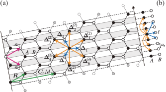
Figure 4: (Color online) (a) An extension of Fig. 1(a) to include the hopping to the second-nearest-neighbor atoms. The three vectors $\bm{\Delta}_{j}$ $(j=1,2,3)$ connect the nearest-neighbor atoms, whereas the six vectors $\bm{\Delta}^{\!\!(2)}_{j}$ $(j=1,2,\ldots,6)$ connect the second-nearest-neighbor ones. (b) An extended 1D lattice model to describe the metallic SWNTs.

V.2 Bulk properties

For the bulk system, the Fourier transformation of $H_{\mu,s}$ along the $\ell$ direction yields the two-by-two Hamiltonian,

$$H_{\mu,s}(k) =\epsilon_{\mu,s}(k;\phi)+\gamma\begin{bmatrix}0&f_{\mu,s}(k;\phi)\\ f_{\mu,s}^{*}(k;\phi)&0\end{bmatrix},$$ (24)

in the sublattice space for the 1D BZ, $-\pi\leq ka_{z}<\pi$, where

$$f_{\mu,s}(k;\phi) =\frac{1}{\gamma}\sum_{j=1}^{3}\gamma^{(1)}_{s,j}{\rm e}^{{\rm i}2\pi\mu\Delta^{\prime\prime}_{j}/d}{\rm e}^{{\rm i}ka_{z}\Delta^{\prime}_{j}},$$ (25)

$$\epsilon_{\mu,s}(k;\phi) =\sum_{j=1}^{6}\gamma^{(2)}_{s,j}{\rm e}^{{\rm i}2\pi\mu\Delta^{\!(2)\prime\prime}_{j}/d}{\rm e}^{{\rm i}ka_{z}\Delta^{\!(2)\prime}_{j}}.$$ (26)

The dispersion relation for subband $(\mu,s)$ is given by

$$E_{\mu,s}(k;\phi) =\epsilon_{\mu,s}(k;\phi)\pm|\gamma f_{\mu,s}(k;\phi)|.$$ (27)

The system is an insulator when $|\epsilon_{\mu,s}(k;\phi)|<|\gamma f_{\mu,s}(k;\phi)|$ in the whole BZ. Thanks to the curvature-induced fine structure, this condition is satisfied even for metallic SWNTs except in the vicinity of $|\phi|=\phi^{*}$, where the band gap is closed by a magnetic field. Then positive and negative $E_{\mu,s}(k)$’s form the conduction and valence bands, respectively. It should be mentioned that $\phi^{*}\ll 1/3$ in metallic SWNTs, which corresponds to the magnetic field of a few Tesla Okuyama2017 .

V.3 Winding number and bulk-edge correspondence

For any SWNT with finite band gap, we can define the winding number as

$$w_{\mu,s}=\frac{1}{2\pi}\oint_{\rm BZ}{\rm d}\arg f_{\mu,s}(k;\phi),$$ (28)

for subband $(\mu,s)$. Strictly speaking, it is a topological invariant only if the sublattice symmetry holds Wen1989 ; Asboth2015 : $\epsilon_{\mu,s}(k;\phi)=0$. However, as far as the system is an insulator, i.e., $|\epsilon_{\mu,s}(k;\phi)|<|\gamma f_{\mu,s}(k;\phi)|$ in the whole BZ, it is well defined. We discuss the topology of metallic SWNTs using $w_{\mu,s}$ in Eq. (28) except for the vicinity of $|\phi|=\phi^{*}$.

The bulk-edge correspondence in Eq. (12) is generalized to

$$N_{\rm edge}=2\sum_{\mu=0}^{d-1}\sum_{s=\pm}|w_{\mu,s}|$$ (29)

in terms of $w_{\mu,s}$. The proof of this relation is given in Appendix B. Although the energy levels of edge states are slightly deviated from $E_{\rm F}=0$ in the presence of $\epsilon_{\mu,s}(k;\phi)$, they are within the band gap as long as the gap remains finite.

V.4 Classification with curvature effects

Now we come to classify the metallic SWNTs. $f_{\mu}(k;\phi)$ defined in Secs. II and III passes the origin on the complex plane for $\mu=\mu_{\pm}$ (at $k=k_{\pm}$) corresponding to the Dirac points in the absence of curvature-induced effects. We evaluate $w_{\mu,s}$ using Eq. (28) around the origin while we can use the results in Table 1 otherwise since the topological nature does not change by a small perturbation. As an example, we show $f_{\mu}(k;\phi)$ on the complex plane for $\mu=0$ in the (7,1)-SWNT (metal-2 with $\mu_{+}=\mu_{-}=0$) in Fig. 5(a). Petals $j=3$ and $5$ go through the origin in the absence of curvature effects, whereas petal $j=4$ winds the origin. The latter yields $w_{\mu}=1$ in Table 1. The contribution from the former is discussed in the following.

In the vicinity of origin on the complex plane,

$$f_{\mu_{\pm},s}(k;\phi)\simeq\frac{\sqrt{3}}{2}a\,{\rm e}^{\pm{\rm i}(\theta-\frac{2\pi}{3})}\bigl{[}(\Delta k_{c}\pm\Delta k_{\rm so}\pm\Delta k_{\phi})$$

$$\quad+{\rm i}(k-k_{\tau}\mp\Delta k_{z})\bigr{]}.$$ (30)

from Eq. (40) in Appendix A. Here, $\Delta k_{\phi}$ represents the AB effect in a magnetic field, $\Delta k_{c}$ and $\Delta k_{z}$ stem from the mixing between $\pi$ and $\sigma$ orbitals, and $\Delta k_{\rm so}$ is due to the SO interaction (see Appendix A). Equation (30) indicates a straight line made by the rotation of angle $\pm(\theta-\frac{2\pi}{3})$ around the origin, from a straight line which intersects orthogonally the real axis at $r=(\Delta k_{c}\pm s\Delta k_{\rm so}\pm\Delta k_{\phi})(\sqrt{3}a/2)$. It gives rise to the winding number when the line intercepts the real axis in the negative part. For armchair SWNTs of $\theta=\pi/6$, this condition is never satisfied since the line is parallel to the real axis. For the other metallic SWNTs, the condition holds if $r>0$, as shown in Fig. 5(b).

In consequence, we obtain the complete expression for $w_{\mu,s}$ for metallic SWNTs. For $\mu\neq\mu_{\pm}$,

$$w_{\mu,s}=w_{\mu}$$ (31)

in Table 1. For $\mu=\mu_{\pm}$,

$$w_{\mu_{\pm},s}=w_{\mu_{\pm}}+\Theta(\Delta k_{c}\pm s\Delta k_{\rm so}\pm\Delta k_{\phi}),$$ (32)

where $w_{\mu_{\pm}}$ is given by Table 1 and $\Theta(x)=1$ ($0$) for $x>0$ ($x<0$). This explains the topological phase transition at $|\phi|\ll 1/3$, which was demonstrated in Ref. Okuyama2017 , for the following reason. $\Delta k_{\phi}$ is proportional to $B$ along the tube axis, $\Delta k_{\phi}=-eBd_{\rm t}/(4\hbar)$, in Eq. (36) in Appendix A. For metallic SWNTs other than the armchair, $\Delta k_{c}\pm s\Delta k_{\rm so}\simeq\Delta k_{c}>0$ and thus Eq. (32) yields $w_{\mu_{\pm},s}=w_{\mu_{\pm}}+1$ at $B=0$. When $B$ is increased beyond $B^{*}$, which satisfies $\Delta k_{c}+s\Delta k_{\rm so}+\Delta k_{\phi}=0$, $w_{\mu_{+},s}$ becomes $w_{\mu_{+}}$.

We obtain the number of edge states $N_{\rm edge}$ through Eq. (29) by the summation of $w_{\mu_{\pm},s}$ in Eqs. (31) and (32). The expression for $N_{\rm edge}$ is common for metal-1 and -2, as shown in Table 2. All the metallic SWNTs but the armchair are a topological insulator in the absence of a magnetic field [Fig. 3(a)] and show the topological phase transition at $B=B^{*}$ [Fig. 3(b)]. The armchair SWNTs are always topologically trivial: They are forbidden to have finite winding numbers regardless of the strength of the magnetic field, which is attributable to the mirror symmetry with respect to a plane including the tube axis Izumida2016 .

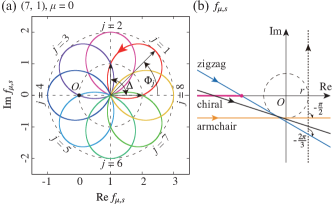
Figure 5: (Color online) (a) $f_{\mu,s}(k)$ on the complex plane for $\mu=0$ in a metallic SWNT with chirality $(7,1)$. $d=1$, $p=1$, and $q=0$. Petals $j=3$ and $5$ pass the origin in the absence of curvature effects, whereas petal $j=4$ rounds the origin. (b) $f_{\mu,s}(k)$ around the origin on the complex plane for $\mu=\mu_{+}$ which passes the $K$ point, in metallic SWNTs with chiral angle $\theta$. $r=(\Delta k_{c}+s\Delta k_{\rm so}+\Delta k_{\phi})(\sqrt{3}a/2)>0$. The dotted line intersects the real axis orthogonally at $r$. The trajectory for a zigzag SWNT ($\theta=0$) is obtained by rotating it by $-2\pi/3$ around the origin (blue line), whereas that for an armchair SWNT ($\theta=\pi/6$) is obtained by rotating it by $-\pi/2$ (orange line). Therefore the intercept of the real axis is always negative (pink segment) for SWNTs of $0\leq\theta<\pi/6$.

VI Discussion

We comment on the previous studies which predicted an increase in the number of edge states in metallic SWNTs as the magnetic field increases Sasaki2005 ; Sasaki2008 ; Marganska2011 . At the first sight, this seems contradictory against our results. However, this is because they use parameters corresponding to $\Delta k_{c}<0$ in our model. We obtain positive $\Delta k_{c}$ by fitting the dispersion relation with that from the ab initio calculation known as the extended tight-binding model Izumida2009 . However, its sign is quite sensitive to the details in the model, and therefore it should be experimentally confirmed which sign is favorable. Also, others theoretically predicted no topological phase transition for metallic SWNTs Lin2016 . This is due to the oversimplification with $\Delta k_{c}=\Delta k_{\rm so}=0$.

A comment should be made on the boundary condition, which is important for the edge states in 1D topological insulators. Our calculations have been performed for finite systems in which a SWNT is cut by a broken line in Fig. 1(a). The angular momentum $\mu$ is a good quantum number in this case. This is a minimal boundary edge, where every atom at the ends has just one dangling bond Akhmerov2008 . The bulk-edge correspondence in Eqs. (12) and (29) holds only for such edges. Some other boundary conditions result in different numbers of edge states, as discussed in Ref. Izumida2016 . Then the winding number $w_{\mu}$ is shifted from that in the case of minimal boundary. Since the shift of $w_{\mu}$ is independent of magnetic field Izumida2016 , the topological phase transition and the critical magnetic field should not be influenced by the boundary conditions. The number of edge states is changed at the transition. For armchair SWNTs, the topological phase transition does not take place with any boundary condition, whereas the number of edge states may be finite. Although the examined boundaries are limited, we speculate that the topological phase transition is determined by the topological nature of the bulk irrespectively of the boundaries in general.

VII Conclusions

We have classified the topology for all possible chiralities $(n,m)$ of SWNTs in the absence and presence of a magnetic field along the tube axis. First, we have studied semiconducting SWNTs using a 1D lattice model in Eq. (6) and depicted in Fig. 1(b). We have found that (i) the semiconducting SWNTs other than $n=m+1$ are topological nontrivial in the absence of a magnetic field and (ii) all the semiconducting SWNTs show the topological phase transition at AB phase $|\phi|=\phi^{*}=1/3$. The phase transition, however, should be hard to observe since a magnetic field of more than $100~{}{\rm T}$ is required when the tube diameter $d_{\rm t}\sim 1~{}{\rm nm}$.

Next, we have examined metallic SWNTs with a small band gap using an extended 1D lattice model in Eq. (23) and depicted in Fig. 4(b). Although the winding number $w_{\mu,s}$ is not a topological invariant in the presence of $\gamma^{(2)}_{s,j}$ in Eq. (23), it is well defined except for the vicinity of topological phase transition. Indeed we have proved the bulk-edge correspondence for $w_{\mu,s}$ in Eq. (29). We have observed that (i) all the metallic SWNTs but the armchair type ($n=m$) are a topological insulator in the absence of a magnetic field and show the topological phase transition at a critical magnetic field $B^{*}$. Since $B^{*}$ can be a few Tesla Okuyama2017 , the topological phase transition could be observed for metallic SWNTs. (ii) The armchair SWNTs are always topologically trivial.

In conclusion, the majority of SWNTs are a topological insulator in the absence of a magnetic field and show a topological phase transition by applying a magnetic field along the tube. Only metallic SWNTs of armchair type are topologically trivial regardless of the magnetic field.

Appendix A Effective lattice model for metallic SWNTs

We construct an effective 1D lattice model for a metallic SWNT, starting from the Hamiltonian of $\bm{k}\cdot\bm{p}$ theory Izumida2009 , as discussed in Ref. Okuyama2017 . In a magnetic field $B$ in the axial direction, the Hamiltonian in the vicinity of $K$ and $K^{\prime}$ points reads

$$\mathcal{H}_{\tau,s}(\bm{k}) =\hbar v_{\rm F}\Bigl{[}\bigl{(}k_{c}-\tau\Delta k_{c}-s\Delta k_{\rm so}-\Delta k_{\phi}\bigr{)}\sigma_{x}$$

$$\quad+\tau\bigl{(}k_{z}-\tau\Delta k_{z}\bigr{)}\sigma_{y}\Bigr{]}+\tau s\epsilon_{\rm so},$$ (33)

with $\sigma_{x}$ and $\sigma_{y}$ being the Pauli matrices in the sublattice space of $A$ and $B$ species. $s=\pm 1$ is the spin in the axial direction, whereas $\tau=\pm 1$ represents $K$ or $K^{\prime}$ valleys. $k_{c}$ and $k_{z}$ are the circumference and axial components of wave number measured from $K$ or $K^{\prime}$ points, respectively. $k_{c}$ is discretized in units of $2\pi/|\bm{C}_{\rm h}|$ while $k_{z}$ is continuous.

In $\mathcal{H}_{\tau,s}(\bm{k})$, the hybridization between $\pi$ and $\sigma$ orbitals appears as the shift of Dirac points from $K$ or $K^{\prime}$ points,

$$\Delta k_{c}=\beta^{\prime}\frac{\cos 3\theta}{d_{\rm t}^{2}},\quad\Delta k_{z}=\zeta\frac{\sin 3\theta}{d_{\rm t}^{2}},$$ (34)

with $\beta^{\prime}=0.0436~{}{\rm nm}$ and $\zeta=-0.185~{}{\rm nm}$. $\Delta k_{c}$ opens a small gap $E_{\rm g}$ except in armchair tubes ($\theta=\pi/6$). The curvature-enhanced SO interaction yields

$$\Delta k_{\rm so}=\alpha^{\prime}_{1}V_{\rm so}\frac{1}{d_{\rm t}},\quad\epsilon_{\rm so}=\alpha_{2}V_{\rm so}\frac{\cos 3\theta}{d_{\rm t}},$$ (35)

with $\alpha^{\prime}_{1}=8.8\times 10^{-5}~{}{\rm meV^{-1}}$, $\alpha_{2}=-0.045~{}{\rm nm}$, and $V_{\rm so}=6~{}{\rm meV}$ being the SO interaction for 2p orbitals in carbon atoms. $\Delta k_{\rm so}$ opens the gap in armchair tubes and gives a correction to $E_{\rm g}$ in the others. The AB phase by the magnetic field $B$ appears as

$$\Delta k_{\phi}=-\frac{eB}{4\hbar}d_{\rm t}.$$ (36)

The band gap is closed at $B^{*}$ when $\tau\Delta k_{c}+s\Delta k_{\rm so}+\Delta k_{\phi}=0$. The last term in $\mathcal{H}_{\tau,s}(\bm{k})$ yields the energy shift from $E_{\rm F}=0$, which is assumed to be small compared with the band gap except in the vicinity of $B=B^{*}$.

The 2D lattice model in Eq. (22) is constructed to reproduce $\mathcal{H}_{\tau,s}(\bm{k})$ around the Dirac points Okuyama2017 . The hopping integral $\gamma^{(1)}_{s,j}$ is given by

$$\gamma^{(1)}_{s,j} =\gamma\exp\left(-{\rm i}\Delta k_{\phi}a_{\text{\tiny CC}}\cos\Theta_{j}\right)\biggl{[}1+\Delta k_{c}a_{\text{\tiny CC}}\sin\Theta_{j}$$

$$\quad-(\Delta k_{z}+{\rm i}s\Delta k_{\rm so})a_{\text{\tiny CC}}\cos\Theta_{j}\biggr{]},$$ (37)

whereas $\gamma^{(2)}_{s,j}$ stems from the SO interaction as

$$\gamma^{(2)}_{s,j}={\rm i}\frac{(-1)^{j+1}}{3\sqrt{3}}s\epsilon_{\rm so}.$$ (38)

In a similar way to Sec. II A, we derive the 1D lattice model in Eq. (23) from Eq. (22). The hopping distance $\Delta^{\prime}_{j}$ and phase factor $\Delta^{\prime\prime}_{j}$ for the nearest-neighbor atoms are given by Eq. (7). For the second-nearest-neighbor atoms, $\Delta^{\!(2)\prime}_{j}$ and $\Delta^{\!(2)\prime\prime}_{j}$ are determined from

$$\bm{\Delta}^{\!\!(2)}_{j}=\Delta^{\!(2)\prime}_{j}\bm{R}+\Delta^{\!(2)\prime\prime}_{j}(\bm{C}_{\rm h}/d).$$ (39)

These quantities are provided in Table 3.

Table 3: Hopping distance and phase factor in the 1D lattice model. Integers $d$, $p$, and $q$ are given by Eqs. (2) and (3).

$j$		1	2	3		$j$		1	2	3	4	5	6
$\Delta^{\prime}_{j}$		0	$\frac{n}{d}$	$-\frac{m}{d}$		$\Delta^{\!(2)\prime}_{j}$		$\frac{m}{d}$	$\frac{n+m}{d}$	$\frac{n}{d}$	$-\frac{m}{d}$	$-\frac{n+m}{d}$	$-\frac{n}{d}$
$\Delta^{\prime\prime}_{j}$		0	$-p$	$q$		$\Delta^{\!(2)\prime\prime}_{j}$		$-q$	$-(p+q)$	$-p$	$q$	$p+q$	$p$

We examine low-lying states near to the $K$ and $K^{\prime}$ points. By expanding the bulk Hamiltonian in Eqs. (24)–(26) around $\mu=\mu_{\tau}$ and $k=k_{\tau}$ in Eqs. (20) and (21), we obtain

$$\gamma f_{\mu,s}(k) =\chi_{\tau}\hbar v_{\rm F}\bigl{[}(k_{c}-\tau\Delta k_{c}-s\Delta k_{\rm so}-\Delta k_{\phi})-{\rm i}\tau(k_{z}-\tau\Delta k_{z})\bigr{]},$$ (40)

$$\epsilon_{\mu,s}(k) =\tau s\epsilon_{\rm so},$$ (41)

with $\chi_{\tau}=\tau{\rm e}^{{\rm i}\tau(\theta-2\pi/3)}$, $k_{c}=(\mu-\mu_{\tau})(2\pi/|\bm{C}_{\rm h}|)$, and $k_{z}=k-k_{\tau}$.

The local band gap around $K$ and $K^{\prime}$ points is evaluated by using Eq. (40). For metallic SWNTs, $k_{c}$ can be zero, and therefore band gap is determined by the curvature effects as

$$E_{\rm g}=\hbar v_{F}\left|\Delta k_{c}+\tau s\Delta k_{\rm so}+\tau\Delta k_{\phi}\right|.$$ (42)

Appendix B Proof of bulk-edge correspondence

In this Appendix, we evaluate the number of edge states from the Schrödinger equation, in a similar manner to Ref. Izumida2016 . For semiconducting SWNTs, edge states have energy $E=E_{\rm F}=0$. For metallic SWNTs, they still have $E=0$ if we set $\epsilon_{\mu,s}(k)=0$ in Eq. (26): The topological nature is determined by $\gamma^{(1)}_{s,j}$, whereas the energy of the edge states is shifted by $\gamma^{(2)}_{s,j}$ in Hamiltonian (22). Here, we examine the edge states at $E=0$, neglecting $\gamma^{(2)}_{s,j}$.

We consider a long but finite SWNT using the 1D lattice model with $\ell=0,1,2,\ldots,L$ in Fig. 4(b). Using the Hamiltonian in Eq. (23), the time-independent Schrödinger equation is written as

$$H_{\mu,s}|\phi\rangle=E|\phi\rangle,\quad|\phi\rangle=\sum_{\sigma=A,B}\sum_{\ell=0}^{L}\phi_{\sigma,\ell}|\sigma,\ell;\mu,s\rangle,$$ (43)

where $|\sigma,\ell;\mu,s\rangle$ is the electronic states at sublattice $\sigma$ of site index $\ell$ with angular momentum $\mu$ and spin $s$. For $E=0$, equations for $\{\phi_{A,\ell}\}$ and $\{\phi_{B,\ell}\}$ are decoupled from each other. We find that the edge states consist of $B$ sublattice ($A$ sublattice) only around $\ell=0$ ($\ell=L$). Here, we examine the former with the boundary conditions of $\phi_{B,-1}=\phi_{B,-2}=\ldots=\phi_{B,-m/d}=0$ because of the hopping integrals from $\ell$ to $\ell+\Delta^{\prime}_{3}=\ell-m/d$ ($\ell\geq 0$). The number of edge states is given by the number of roots in the equation that decay into the tube body, subtracted by the number of boundary conditions, $m/d$.

If we assume a wave function in a form of $\phi_{\sigma,\ell}=\lambda^{\ell}\phi_{\sigma,0}$ with a complex number $\lambda$, the equation for $B$ sublattice reads,

$$\sum_{j=1}^{3}\gamma^{(1)}_{s,j}{\rm e}^{{\rm i}2\pi\mu\Delta^{\prime\prime}_{j}/d}\lambda^{\Delta^{\prime}_{j}}=0.$$ (44)

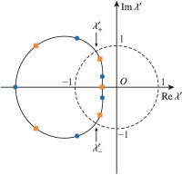
Figure 6: (Color online) Zero-energy modes at $B$ sublattice in the $(6,4)$-SWNT on the complex plane of $\lambda^{\prime}$ in Eq. (47). Circles and squares correspond to modes of $\mu=0$ and $1$, respectively. The solid line shows Eq. (48), whereas the broken line shows a unit circle centered at the origin. They are crossed at $\lambda^{\prime}_{\pm}={\rm e}^{{\rm i}2\pi/3}$.

First, we neglect the curvature-induced effects and only the AB phase is taken into account, i.e., $\gamma^{(1)}_{s,j}=\gamma\exp\left({\rm i}2\pi\phi\frac{a_{\rm CC}\cos\Theta_{j}}{\pi d_{\rm t}}\right)=\gamma\exp\left(-{\rm i}\Delta k_{\phi}a_{\rm CC}\cos\Theta_{j}\right)$. From Eq. (44), we obtain

$$1 +{\rm e}^{-{\rm i}2\pi p\mu/d}{\rm e}^{-{\rm i}(n+2m)\phi a^{2}/(4S)}\lambda^{n/d}$$

$$+{\rm e}^{{\rm i}2\pi q\mu/d}{\rm e}^{-{\rm i}(2n+m)\phi a^{2}/(4S)}\lambda^{-m/d}=0,$$ (45)

with $S=\pi(d_{\rm t}/2)^{2}$ being the cross section of a SWNT. Then a straightforward calculation yields

$${\rm e}^{{\rm i}2\pi(\mu+\phi)/d}\left(\lambda^{\prime}\right)^{m/d}=\left(-1-\lambda^{\prime}\right)^{\frac{n+m}{d}},$$ (46)

where

$$\lambda^{\prime}={\rm e}^{-{\rm i}2\pi(p+q)\mu/d}{\rm e}^{{\rm i}(n-m)\phi a^{2}/(4S)}\lambda^{\frac{n+m}{d}}.$$ (47)

Equation (46) yields two equations for absolute and phase values as

$$\left|\lambda^{\prime}\right|^{m/d}=\left|-1-\lambda^{\prime}\right|^{\frac{n+m}{d}},$$ (48)

$$\frac{n+m}{d}\arg\left(-1-\lambda^{\prime}\right)-\frac{m}{d}\arg\lambda^{\prime}-\frac{2\pi(\mu+\phi)}{d}=2\pi j,$$ (49)

with $j$ being an arbitrary integer. The condition Eq. (48) gives a closed loop on the complex plane of $\lambda^{\prime}$, which crosses the unit circle of $\left|\lambda^{\prime}\right|=1$ at $\lambda^{\prime}_{\pm}={\rm e}^{\pm{\rm i}2\pi/3},$ as shown in Fig. 6. On the loop, Eq. (49) indicates $\frac{n+m}{d}$ points, which are the solution of Eq. (46). Among them, decaying modes from $\ell=0$ correspond to the points of $|\lambda|=\left|\lambda^{\prime}\right|<1$. We obtain the number of such modes by counting integers between $j_{+}$ and $j_{-}$, where

$$j_{+}=\frac{2n+m}{3d}-\frac{\mu+\phi}{d},\quad j_{-}=\frac{n-m}{3d}-\frac{\mu+\phi}{d}$$ (50)

satisfy Eq. (49) with $\lambda^{\prime}_{\pm}$.

For metallic SWNTs, $j_{\pm}$ in Eq. (50) can be integers for $\phi=0$, which correspond to $K$ and $K^{\prime}$ points. We neglect their contribution for now, and examine later.

The above-mentioned analysis yields the number of roots of Eq. (44). The subtraction of $m/d$ determines the number of edge states around $\ell=0$ with angular momentum $\mu$, $N_{{\rm edge},\mu}$, for each spin. $N_{{\rm edge},\mu}$ coincides with $|w_{\mu}|$ in Table 1. The same calculation can be applied for the edge states around $\ell=L$, which consist of $A$ sublattice. In consequence, $4N_{{\rm edge},\,\mu}$ gives the total number of edge states, which yields the bulk-edge correspondence in Eq. (12).

As an example, Fig. 6 depicts the edge modes around $\ell=0$ in the $(6,4)$-SWNT $(d=2)$ on the $\lambda^{\prime}$ plane. Circles and squares are modes of $\mu=0$ and $1$, respectively. Solid and broken lines show Eq. (48) and the unit circle $|\lambda^{\prime}|=1$, respectively. For $\mu=0$, the number of the modes inside the broken line is two. Since the number of boundary conditions is $m/d=2$, we have $2-2=0$ edge states, which corresponds to $w_{\mu=0}=0$. For $\mu=1$, on the other hand, we have three decaying modes and hence one edge state, which is consistent with $w_{\mu=1}=1$.

Finally, we examine the contribution from $K$ and $K^{\prime}$ points in metallic SWNTs. Note that if we write $\lambda={\rm e}^{({\rm i}k-\kappa)a_{z}}$, Eq. (44) results in the condition of $\left.f_{\mu,s}(k)\right|_{k\rightarrow k+{\rm i}\kappa}=0$. Without the curvature-induced effects, a plane wave gives its solution. Thus we examine how the wave function is modified when the curvature-induced effects are included. From Eq. (40), we find a solution near $K$ and $K^{\prime}$ points with $\lambda={\rm e}^{({\rm i}k-\kappa)a_{z}}$,

$$k=k_{\tau}+\tau\Delta k_{z},\quad\kappa=\Delta k_{c}+\tau s\Delta k_{\rm so}+\tau\Delta k_{\phi}.$$ (51)

Then we find that there is one additional edge state at $B$ sublattice around $\ell=0$ if $\kappa>0$. This ends up the conclusion that $N_{\rm edge}$ in Table 2 is valid also for metallic SWNTs. Thus the bulk-edge correspondence is established for both semiconducting and metallic SWNTs in an arbitrary magnetic field.

References

- (1) R. Saito, G. Dresselhaus, and M. S. Dresselhaus, Physical properties of carbon nanotubes (Imperial College Press, London, 1998).
- (2) N. Hamada, S. Sawada, and A. Oshiyama, “New one-dimensional conductors: Graphitic microtubules”, Phys. Rev. Lett. 68, 1579 (1992).
- (3) R. Saito, M. Fujita, G. Dresselhaus, and M. S. Dresselhaus, “Electronic structure of graphene tubules based on C60”, Phys. Rev. B 46, 1804 (1992).
- (4) C. L. Kane and E. J. Mele, “Size, Shape, and Low Energy Electronic Structure of Carbon Nanotubes”, Phys. Rev. Lett. 78, 1932 (1997).
- (5) T. Ando, “Spin-orbit interaction in carbon nanotubes”, J. Phys. Soc. Jpn 69, 1757 (2000).
- (6) J. Klinovaja, S. Gangadharaiah, and D. Loss, “Electric-Field-Induced Majorana Fermions in Armchair Carbon Nanotubes”, Phys. Rev. Lett. 108, 196804 (2012).
- (7) R. Egger and K. Flensberg, “Emerging Dirac and Majorana fermions for carbon nanotubes with proximity-induced pairing and spiral magnetic field”, Phys. Rev. B 85, 235462 (2012).
- (8) J. D. Sau and S. Tewari, “Topological superconducting state and Majorana fermions in carbon nanotubes”, Phys. Rev. B 88, 054503 (2013).
- (9) C.-H. Hsu, P. Stano, J. Klinovaja, and D. Loss, “Antiferromagnetic nuclear spin helix and topological superconductivity in 13C nanotubes”, Phys. Rev. B 92, 235435 (2015).
- (10) W. Izumida, R. Okuyama, A. Yamakage, and R. Saito, “Angular momentum and topology in semiconducting single-wall carbon nanotubes”, Phys. Rev. B 93, 195442 (2016).
- (11) S. Lin, G. Zhang, C. Li, and Z. Song, “Magnetic-flux-driven topological quantum phase transition and manipulation of perfect edge states in graphene tube”, Sci. Rep. 6, 31953 (2016).
- (12) R. Okuyama, W. Izumida, and M. Eto, “Topological Phase Transition in Metallic Single-Wall Carbon Nanotube”, J. Phys. Soc. Jpn 86, 013702 (2017).
- (13) W. Izumida, L. Milz, M. Marganska, and M. Grifoni, “Topology and zero energy edge states in carbon nanotubes with superconducting pairing”, Phys. Rev. B 96, 125414 (2017).
- (14) M. Marganska, L. Milz, W. Izumida, C. Strunk, and M. Grifoni, “Majorana quasiparticles in semiconducting carbon nanotubes”, Phys. Rev. B 97, 075141 (2018).
- (15) X. Zang, N. Singh, and U. Schwingenschl, “Topological characterization of carbon nanotubes”, J. Phys.: Cond. Matt. 30, 335301 (2018).
- (16) X. G. Wen and A. Zee, “Winding number, family index theorem, and electron hopping in a magnetic field”, Nucl. Phys. B 316, 641 (1989).
- (17) A. P. Schnyder, S. Ryu, A. Furusaki, and A. W. W. Ludwig, “Classification of topological insulators and superconductors”, Phys. Rev. B 78, 195125 (2008).
- (18) Y. Kobayashi, K. Fukui, T. Enoki, K. Kusakabe, and Y. Kaburagi, “Observation of zigzag and armchair edges of graphite using scanning tunneling microscopy and spectroscopy”, Phys. Rev. B 71, 193406 (2005).
- (19) K. Sasaki, S. Murakami, R. Saito, and Y. Kawazoe, “Controlling edge states of zigzag carbon nanotubes by the Aharonov-Bohm flux”, Phys. Rev. B 71, 195401 (2005).
- (20) K. Sasaki, M. Suzuki, and R. Saito, “Aharanov-Bohm effect for the edge states of zigzag carbon nanotubes”, Phys. Rev. B 77, 045138 (2008).
- (21) M. Margańska, M. del Valle, S. H. Jhang, C. Strunk, and M. Grifoni, “Localization induced by magnetic fields in carbon nanotubes”, Phys. Rev. B 83, 193407 (2011).
- (22) C. T. White, D. H. Robertson, and J. W. Mintmire, “Helical and rotational symmetries of nanoscale graphitic tubules”, Phys. Rev. B 47, 5485 (1993).
- (23) R. A. Jishi, M. S. Dresselhaus, and G. Dresselhaus, “Symmetry properties of chiral carbon nanotube”, Phys. Rev. B 47, 16671 (1993).
- (24) A. R. Akhmerov and C. W. J. Beenakker, “Boundary conditions for Dirac fermions on a terminated honeycomb lattice”, Phys. Rev. B 77, 085423 (2008).
- (25) H. Ajiki and T. Ando, “Electronic states of carbon nanotubes”, J. Phys. Soc. Jpn 62, 1255 (1993).
- (26) W. Izumida, K. Sato, and R. Saito, “Spin-orbit interaction in single wall carbon nanotubes: Symmetry adapted tight-binding calculation and effective model analysis”, J. Phys. Soc. Jpn 78, 074707 (2009).
- (27) J. K. Asbóth, L. Oroszlány, and A. Pályi, A short course on topological insulators: Band-structure topology and edge states in one and two dimensions (Springer, Berlin, 2015).