Intrinsic and extrinsic geometries of correlated many-body states

Abstract

We explore two approaches to characterise the quantum geometry of the ground state of correlated fermions in terms of the distance matrix in the spectral parameter space. (a) An intrinsic geometry approach, in which we study the intrinsic curvature defined in terms of the distance matrix. (b) An extrinsic geometry approach, in which we investigate how the distance matrix can be approximately embedded in finite dimensional Euclidean spaces. We implement these approaches for the ground state of a system of one-dimensional fermions on a 18-site lattice with nearest neighbour repulsion. The intrinsic curvature sharply changes around the Fermi points in the metallic regime but is more or less uniform in the insulating regime. In the metallic regime, the embedded points clump into two well seperated sets, one corresponding to modes in the Fermi sea and the other to the modes outside it. In the insulating regime, the two sets tend to merge.

I Introduction

In the past few decades, there has been a body of work attempting to characterise many-body states using the concepts of quantum geometry Resta and Sorella (1999); Resta (2002); Haldane (2004). The symmetries of the ground states of many-body systems, characterised by the expectation values of local order parameters have proven to be a very useful way to characterise the phases of the systems Landau (1937). However, in several cases this is inadequate. There can be two phases of the system with very different physical properties but with the same symmetry. The metallic and insulating phases of a solid are the prime example of such a situation. These two phases can be distinguished by the nature of the excited states of the system. The metallic state has gapless charged excitations whereas the charged excitations in the insulating phase have a gap.

In a seminal paper, Walter Kohn Kohn (1964) suggested that it is possible to distinguish these two phases by examining the structure of the ground state alone. Namely, given only the ground state, it is possible to predict if the system is metallic or insulating. Kohn also gave a qualitative description of what distinguishes the ground state of a metal and an insulator. This idea has been followed up by others Aligia and Ortiz (1999); Resta and Sorella (1999); Resta (2002, 2011), and it has been been argued that this difference can be quantified using the concepts of quantum geometry.

In particular, it has been shown that the so called localisation tensor, the second moment of the pair correlation function in the ground state is a quantity that distinguishes between the two phases and characterises the insulating phase. It is divergent in the metallic phase and finite in the insulating phase. Further its value in the insulating phase is a measure of the localisation of the electrons Resta and Sorella (1999); Souza et al. (2000); Resta (2011). It has also been shown that for mean field states corresponding to filled bands, the localisation tensor is the integral of the quantum metric corresponding to the filled bands over the Brilliuon zone Resta (2002); Sgiarovello et al. (2001). This result establishes the relation of the metallic/insulating property of the system to the quantum geometry for band insulators which are well described by mean field states.

In previous work Hassan et al. (2018), we had given a definition of quantum distances in the space of spectral parameters for general many particle states. For fermions in a periodic potential, the spectral parameters are the quasi-momenta in the Brillioun zone. We had shown that our definition satisfies the triangle inequalities and reduces to the standard definition, in terms of the single particle wave functions for mean-field states.

An important feature of our definition is that it gives sensible and nontrivial results for the distance matrix in the space of spectral parameters for systems with partially filled bands. Thus, unlike the previous studies, our formalism enables us to probe the quantum geometry of many-body states both in the metallic phase and in the insulating phase.

In this paper, we attempt to find ways to characterise the quantum geometry of many-fermion states in terms of its distance matrix. We explore two approaches. First, we study the intrinsic curvature implied by the distance matrix. Next, we study an approximate embedding of the distance matrix in low dimensional Euclidean spaces which gives a visualization of the ground state.

How are these geometric quantities related to the physics of the system? We do not have general results on this issue just now, but discuss it in the context of the known physics of a specific, well studied, model of interacting fermions, the one-dimensional $t$-$V$ model at half filling, a model of spinless fermions on a lattice with nearest neighbour repulsion Yang and Yang (1966); Baxter (1982); Cazalilla et al. (2011). At $V/t=2$, this model has a metal-insulator transition Shankar (1990). At $V=0$ it is a trivial Fermi liquid, at $0<V/t<2$ it is a metallic Luttinger liquid and at $V/t>2$, it is an insulator. We solve this model numerically for 18 sites. Since it is a finite size system, there is no phase transition but only a crossover. We compute the different geometric quantities that characterise the ground state and analyse how they differ in the two regimes.

The rest of the paper is organised as follows. In Section II, we review our definition of quantum distances in the spectral parameter space. In the model we study, these parameters are the quasi-momenta taking values in the Brillioun zone ($BZ$). As mentioned above, we are studying finite size model. Thus the quasi-momenta are discrete and finite. We therefore need the techniques of discrete geometry to study the system. The model and the mathematical notations to study its geometry are also described in this section. The definition that we use for the intrinsic curvature of a discrete set is discussed in Section III. This section also presents the results of the computation of the curvature in our model and its relation to the physics of the system. In Section IV we motivate our attempts to approximately embed the distance matrix in a Euclidean space. In Section IV.1, we review the fact that, for mean field states, our definition of quantum distances reduces to the standard Hilbert-Schmidt distances in terms of the single particle wave functions. We then show that, in general, Hilbert-Schmidt distances in a finite dimensional Hilbert space can be isometrically embedded in a finite dimensional Euclidean space. In Section IV.2, we review the techniques of embedding a general distance matrix in a Euclidean space. Section IV.3 implements the procedure analytically for the two extreme limits of the coupling constant, $V=0,\infty$. The numerical results for finite, non-zero $V$ are presented in Section IV.4. Section V discusses the concept of approximate embedding in finite dimensional Euclidean spaces. Section VI discusses the Euclidean embedding for the so called Wasserstein distance matrix, a quantity we use to define the intrinsic curvature. We summarise our results and discuss the conclusions we draw from them in Section VII.

II Definitions, conventions and notation

In this section we first review our definition of the distance matrix between pair of points in the spectral parameter space for correlated states Hassan et al. (2018). We define the notion of a graph associated with a state of a finite dimensional system. We then describe the details of the model that we study by numerical exact diagonalization.

II.1 The distance matrix

In previous work Hassan et al. (2018), we had defined the quantum distance $d(\mathbf{k}_{i},\mathbf{k}_{j})$ between two points $\mathbf{k}_{i}$ and $\mathbf{k}_{j}$ in the spectral parameter space in terms of the expectation values of what we called the exchange operators. We review that definition below.

We consider a tight binding model on a Bravais lattice with $N_{B}$ sub-lattices labelled by $\alpha$. We label the points on the $BZ$ by $l$ (an integer) and denote the occupation number of the $(\mathbf{k}_{l},\alpha)$ mode by $n_{\mathbf{k}_{l}\alpha}$. The collection of all the occupation numbers is denoted by $\left\{n\right\}$. The empty state ($n_{\mathbf{k}_{l}\alpha}=0,~{}\forall\mathbf{k}_{l},\alpha$) is denoted by $|0\rangle$. The Fock basis is,

$$|\left\{n\right\}\rangle=\prod_{l,\alpha}\left(C^{\dagger}_{\mathbf{k}_{l}\alpha}\right)^{n_{\mathbf{k}_{l}}}|0\rangle,~{}~{}C^{\dagger}_{\mathbf{k}_{l}\alpha}C_{\mathbf{k}_{l}\alpha}|\left\{n\right\}\rangle=n_{\mathbf{k}_{l}\alpha}|\left\{n\right\}\rangle$$ (1)

where $(C^{\dagger}_{\mathbf{k}_{l}\alpha},C_{\mathbf{k}_{l}\alpha}),~{}\alpha=1,\dots,N_{B}$ are the fermion creation and annihilation operators.

Any many-body state, $|\psi\rangle$ can be expanded as,

$$|\psi\rangle=\sum_{\{n\}}\psi(\{n\})|\{n\}\rangle.$$ (2)

We define the exchange operators, $E(\mathbf{k}_{i},\mathbf{k}_{j})$, by their action on the Fock basis. These operators exchange the occupation numbers of the modes at $\mathbf{k}_{i}$ and $\mathbf{k}_{j}$. We define,

$$E(\mathbf{k}_{i},\mathbf{k}_{j})|\dots,n_{\mathbf{k}_{i}},\dots,n_{\mathbf{k}_{j}},\dots\rangle\equiv|..,n_{\mathbf{k}_{j}},..,n_{\mathbf{k}_{i}},..\rangle.$$ (3)

The quantum distance between $\mathbf{k}_{i}$ and $\mathbf{k}_{j}$ is then defined as,

$$d(\mathbf{k}_{i},\mathbf{k}_{j})\equiv\sqrt{1-|\langle\psi|E(\mathbf{k}_{i},\mathbf{k}_{j})|\psi\rangle|^{\alpha}}.$$ (4)

The above definition satisfies all the properties of distances including triangle inequalities Hassan et al. (2018). For a $d$-dimensional lattice with $L^{d}$ number of total sites, with every $d$ dimensional vector $\mathbf{k}_{i}=(k_{i}^{1},k_{i}^{2},\dots k_{i}^{d})$ representing a point in the spectral parameter space $\mathbf{k}_{i}\in\mathbf{k}$, we associate a unique integer $i$, which runs from $1$ to $L^{d}$. So the above distances defined in Eq. (4), gives us a $L^{d}\times L^{d}$ distance matrix $D$ whose elements are given by

$$D(i,j)\equiv\sqrt{1-|\langle\psi|E(\mathbf{k}_{i},\mathbf{k}_{j})|\psi\rangle|^{\alpha}}.$$ (5)

II.2 The graph of a state

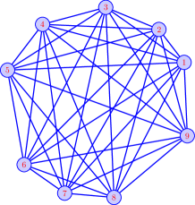
Figure 1: The schematic representation of the graph of a 9-site system.

In this paper, all our explicit computations are for a finite site system detailed below. Thus we consider the problem of extracting geometric information from a $L^{d}\times L^{d}$ distance matrix $D$, of a many-body state, defined between any two points on the set of quasi-momenta, denoted by $BZ$. We refer to the combination, $G\equiv(BZ,D)$ as the graph of the state. The quasi-momenta are the vertices of the graph. Any pair of quasi-momenta define an edge and $D$ defines the length, of each edge. Fig. (1) shows the schematic figure for a graph of a 9-site system.

II.3 The 1-dimensional $t$-$V$ model

As mentioned above, we study a single band model on a one dimensional lattice consisting of $L$ sites with nearest neighbour repulsive interactions, the so called $t$-$V$ model. The Hamiltonian is

$$H = H_{0}+H_{int}$$ (6)

$$H_{0} = -t\sum_{i=1}^{L}\left(C_{i}^{\dagger}C_{i+i}+H.c.\right)$$ (7)

$$H_{int} = V\sum_{i=1}^{L}~{}n_{i}n_{i+1}$$ (8)

where $n_{i}\equiv C^{\dagger}_{i}C_{i}$ and we impose the periodic boundary conditions, $C_{i+L}=C_{i}$. The (dimensionless) quasi-momenta can then be chosen to be $q_{k}=\frac{2\pi}{L}k,~{}k=1,\dots,L$. The operators that create and annihilate fermions with quasi-momentum $q_{k}$ are

$$C^{\dagger}_{k} \equiv \frac{1}{\sqrt{L}}\sum_{i=1}^{L}~{}e^{-iq_{k}i}C^{\dagger}_{i}$$ (9)

$$C_{k} \equiv \frac{1}{\sqrt{L}}\sum_{i=1}^{L}~{}e^{iq_{k}i}C_{i}.$$ (10)

In this one band model, for translationally invariant states, the expression for the expectation values of the exchange operators in terms of the fermion operators has been shown to be Hassan et al. (2018),

$$\langle\psi|E(k_{1},k_{2})|\psi\rangle=1-\langle\psi|\left(n_{k_{1}}-n_{k_{2}}\right)^{2}|\psi\rangle$$ (11)

where $n_{k}\equiv C^{\dagger}_{k}C_{k}$.

As described in our previous paper Hassan et al. (2018), we have solved for the ground state of this model numerically for $L\leq 18$ and $V\leq 12$.

III The intrinsic curvature

In the thermodynamic limit, the $BZ$ is a continuous manifold (topologically, a torus). If the distance matrix $D(\mathbf{k}_{1},\mathbf{k}_{2})$ is a smooth function of its arguments, then local geometric objects like the metric and curvature can be defined by standard methods.

For finite-site correlated systems, the $BZ$ is a discrete and finite set. We do not have a continuous manifold but only a graph as defined above. Various definitions have been proposed for the notion of curvature for a graph Saucan and Appleboim (2009); Forman (2003); Ollivier (2009, 2010). In this work, we use the defintion of the curvature proposed by Ollivier, for a graph Ollivier (2010); Lin et al. (2011), called the Ollivier-Ricci Curvature.

III.1 The Ollivier-Ricci curvature of a graph

The definition of the Ollivier-Ricci curvature for a graph is motivated by the following definition of the Ricci curvature of a continuous manifold Ollivier (2013).

Consider a smooth, $N$-dimensional Riemannian manifold $\mathcal{M}$. Denote the local coordinates by $x^{\mu},~{}\mu=1,\dots,N$ and the metric by $g_{\mu\nu}(\mathbf{x})$. Consider a nearby point with local coordinates $\mathbf{y}=\mathbf{x}+\delta\mathbf{v}$, where $\mathbf{v}$ is a unit tangent vector at $\mathbf{x}$. Define two $\epsilon$-balls, $m_{x}^{\epsilon}$ and $m_{y}^{\epsilon}$ around $\mathbf{x}$ and $\mathbf{y}$ to consist of the points in $\mathcal{M}$ that are at a distance $\leq\epsilon$ from $\mathbf{x}$ and $\mathbf{y}$ respectively.

Figure 2: Two nearby balls, $m_{x}^{\epsilon}$ and $m_{y}^{\epsilon}$ of radius $\epsilon$ whose centres are a small distance, $\delta$, apart, along the unit vector $\mathbf{v}$. Parallel transport of a unit vector $\mathbf{w}$ gives $\mathbf{w}^{\prime}$ such that for a point $p\in m_{x}^{\epsilon}$ parallel transport along the geodesic of length $\delta$ yields a point $p^{\prime}\in m_{y}^{\epsilon}$. The average distance between the points $p$ and $p^{\prime}$ in flat space is equal to $\delta$, while in the presence of curvature the lowest-order deviation from $\delta$ is given by Equation (12).

It has been been shown Ollivier (2013) that if $m_{x}^{\epsilon}$ is mapped to $m_{y}^{\epsilon}$ using the Levi-Civita connection, then the average distance between the points $p\in m_{x}^{\epsilon}$ and their images $p^{\prime}\in m_{y}^{\epsilon}$, in the limit $\delta,\epsilon\rightarrow 0$, is

$$W(m_{x}^{\epsilon},m_{y}^{\epsilon})=\delta(1-\frac{1}{2(N+2)}\kappa(\mathbf{v},\mathbf{v})+O(\epsilon^{3}+\delta\epsilon^{2})),$$ (12)

where $\kappa(\mathbf{v},\mathbf{v})$ is the Ricci curvature associated with the unit vector $\mathbf{v}$. This is schematically illustrated in Figure (2).

The above discussion motivates the definition of the curvature of graphs as follows Ollivier (2013); Lin et al. (2011). Replace the $\epsilon$-ball, $m_{x}^{\epsilon}$ around $\mathbf{x}$ by the normalised distribution of distances of all the vertices in the graph from the vertex $i$,

$$m_{i}(j)=\frac{D(i,j)}{\sum_{k}D(i,k)}.$$ (13)

Replace the average distance $W$ by the so called Wasserstein distance, $W(m_{i},m_{j})$, defined as the distance between two distributions, $m_{i}$ and $m_{j}$ as follows Villani (2008):

$$W(m_{i},m_{j})\equiv\inf_{\Pi}\sum_{kl}D(k,l)\Pi_{ij}(k,l)$$ (14)

where $\Pi_{ij}(k,l)$ is a joint probability distribution defined by,

$$\sum_{l}\Pi_{ij}(k,l)=m_{i}(k),~{}~{}\sum_{k}\Pi_{ij}(k,l)=m_{j}(l).$$ (15)

The curvature, $\kappa(i,j)$, corresponding an edge $(i,j)$ of the graph is then defined by,

$$W(m_{i},m_{j})=D(i,j)(1-\kappa(i,j)).$$ (16)

The corresponding generalization of the scalar curvature at a point $\mathbf{x}$ in Riemannian manifold for a graph is Jost and Liu (2014)

$$\kappa(i)=\frac{1}{\sum_{k}D(i,k)}\sum_{j}\kappa(i,j).$$ (17)

III.2 Numerical results for the intrinsic curvature

We have numerically computed the ground state of the Hamiltonian of the 1-dimensional $t$-$V$ model defined in Section II.3 for $L=18$. We have then computed the $18\times 18$ distance matrix, $D(i,j)$, as defined by Equations (3) and (4). We have choosen $\alpha=2$ in Eq. (5) to obtain the distance matrix.

The problem of computing the Wasserstein distance, $W(m_{i},m_{j})$, is a problem in linear programming Loisel and Romon (2014). We have to minimize the linear function of $\pi_{ij}$ given in Equation (14), subject to linear constraints given in Equation (15). We do this numerically, using the standard techniques of linear programming.

The curvature along each edge of the graph defined in Equation (16) and the scalar curvature defined in Equation (17) are then computed.

To characterise the values of curvatures along the edges in the metallic state, we find it convenient to classify the edges into two types, as follows. The non-interacting system defines a Fermi sea of occupied single particle states. We denote the quasi-momenta of the occupied states by $k_{in}$ and the quasi-momenta of the unoccupied states by $k_{out}$.

In the metallic regime, $V\ll 2$, we find that the curvatures classify the edges into two classes, $e_{1}\equiv(k_{in},k_{in})$ or ($k_{out},k_{out}$) and $e_{2}\equiv(k_{in},k_{out})$ or ($k_{out},k_{in}$). The edges $e_{1}$ have large curvatures whereas the edges $e_{2}$ have small curvatures. On the other hand the curvatures of $e_{1}$ and $e_{2}$ are both quite large and uniform in the insulating regime, $V\gg 2$. This is illustrated in Figure (3). Fig. (4) shows the Ricci curvature of both type of edges as a function of $V$. The curvature of $e_{1}$ is more or less constant at all the values of the interaction. However, in the metallic and the cross over regime, the curvature of $e_{2}$ is continously changing. After the cross over it saturates to a constant value, approximately the same as $e_{1}$.

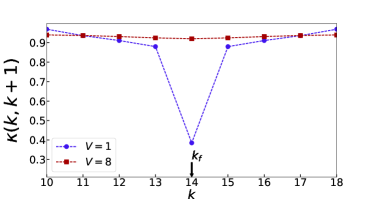
Figure 3: Curvatures for the nearest neighbour edges ($k,k+1$) over half the $BZ$, where $k$ are the quasi-momenta modes corresponding to the vertices of the graph, for different interaction strengths. The metallic regime is characterised by a discontinuity at the Fermi point $k_{f}$.

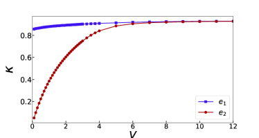
Figure 4: Curvatures for both type of edges $e_{1}$ and $e_{2}$ as function of interaction strength $V$.

Fig. (3) shows the plot of curvature for nearest neighbour edges $\kappa(k,k+1)$ in the two regimes. It can be seen for $V=1$, in the metallic regime there is a discontinuity in the curvature, at the Fermi point which is labelled by $k_{f}$. This discontinuity decreases as function of interaction strength and vanishes at large $V$. The insulating regime is characterised by a uniform scalar curvature, whereas the scalar curvature varies considerably for different vertices in the metallic phase. This is illustrated in Fig. (5) which shows the plot of the scalar curvature as a function of the quasi-momenta modes.

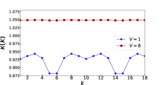
Figure 5: Scalar Curvature as a function of the quasi-momenta modes representing vertices of the graph. In insulating regime the scalar curvature is uniform over all the vertices.

Thus the “clustering” of the distances in metallic phase that we find in our previous study Hassan et al. (2018) manifests in the Ricci curvature by distinct differences in the curvature along the two different types of edges, $e_{1}$ and $e_{2}$. We also find a variable scalar curvature in this phase. The “declustered” uniform distances in the insulating regime found in our previous work Hassan et al. (2018) manifests as homogenous curvatures.

IV Isometric embedding of the distance matrix in a Euclidean space

In this section we explore the extrinsic geometry of the distance matrix by isometrically embedding it in a Euclidean space. Namely, we attempt to find a set of points, $\mathbf{x}_{i}$, in some Euclidean space such that,

$$D(i,j)=|\mathbf{x}_{i}-\mathbf{x}_{j}|.$$ (18)

First, we show that the distance matrices of mean field states can always be embedded in a finite dimensional Euclidean space. Then, we examine the general method of isometrically embedding a distance matrix in a Euclidean space. We follow this by exact analytical results for the extreme values of the coupling, namely $V=0,\infty$. Finally, we apply the method to the numerically computed distance matrix of the 18-site $t$-$V$ model.

IV.1 Embedding of mean field states

In previous work Hassan et al. (2018) we had shown that for a tight binding model with one band completely filled and the others completely empty, our definition of the quantum distance matrix, in terms of the expectation values of the exchange operators reduces to the standard definition in terms of one particle wavefunctions. In Appendix A, we generalise this result to the case of a general mean field state with several filled and partially filled bands. In particular, we show that for the case of the mean field states of an $N_{B}$ band tight binding model, with $N_{F}(\mathbf{k})$ of the bands occupied at $\mathbf{k}\in BZ$, the distance matrix is,

$$D_{\alpha}(\mathbf{k}_{1},\mathbf{k}_{2}) = \sqrt{1-|\langle\Psi(\mathbf{k}_{1})|\Psi(\mathbf{k}_{2})\rangle|^{2\alpha}\delta_{N_{F}(\mathbf{k}_{1}),N_{F}(\mathbf{k}_{2})}}$$

where $|\Psi(\mathbf{k})\rangle$ is the Slater determinant of the occupied single particle wave functions at $\mathbf{k}$.

In this section, we show that, at $\alpha=1$, namely the Hilbert-Schmidt distance matrix, in a finite dimensional Hilbert space can always be isometrically embedded in a finite dimensional Euclidean space. We further show that for arbitrary $\alpha$, while the embedding in a finite dimensional Euclidean space is not isometric, the metric, which gives the distance between two infinitesimally nearby points, is the same for all $\alpha$ up to a scaling factor.

We consider a $N$-dimensional Hilbert space, ${\cal H}_{N}$. The matrix of Hilbert-Schmidt distances between $|\Psi_{n}\rangle,~{}|\Psi_{m}\rangle\in{\cal H}_{N}$, is

$$(D(n,m))^{2}=1-{\rm tr}\left(\rho_{n}\rho_{m}\right)$$ (19)

where $\rho_{n}\equiv|\Psi_{n}\rangle\langle\Psi_{n}|$.

Any linear Hermitian operator in ${\cal H}_{N}$ can be expressed as a linear combination of the $N^{2}$ generators of $U(N)$ in the fundamental representation. We can always take these to be the identity operator, $I$, and the generators of $SU(N)$, $T^{\alpha},~{}\alpha=1,\dots,N^{2}-1$. These can be chosen to satisfy the conditions

$$\left(T^{\alpha}\right)^{\dagger}=T^{\alpha},~{}~{}~{}{\rm tr}\left(T^{\alpha}\right)=0,~{}~{}~{}\frac{1}{2}{\rm tr}\left(T^{\alpha}T^{\beta}\right)=\delta^{\alpha\beta}.$$ (20)

We can express $\rho_{n}$ as,

$$\rho_{n}=\frac{1}{N}+\vec{a}_{n}\cdot\vec{T},~{}~{}~{}~{}~{}a_{n}^{\alpha}=\frac{1}{2}{\rm tr}\left(T^{\alpha}\rho_{n}\right).$$ (21)

Since $T^{\alpha}$ and $\rho_{n}$ are Hermitian matrices, $\vec{a}$ is a real $N^{2}-1$ dimensional vector, i.e $\vec{a}_{n}\in\mathbb{R}^{(N^{2}-1)}$.

The fact that $\rho^{2}_{n}=\rho_{n}$ and ${\rm tr}\rho_{n}=1$ implies that

$$\vec{a}_{n}\cdot\vec{a}_{n}=\frac{1}{2}\left(1-\frac{1}{N}\right).$$ (22)

Note that $\rho_{n}^{2}=\rho_{n}$ implies other constraints on $\vec{a}_{n}$ as well but these are not relevant for the current proof.

The square of the above matrix is computed to be,

$$(D(n,m))^{2} = 1-\frac{1}{N}-2\vec{a}_{n}\cdot\vec{a}_{m}$$ (23)

$$= |\vec{a}_{n}-\vec{a}_{m}|^{2}.$$ (24)

Thus we have shown that the Hilbert-Schmidt distance matrix of mean field states can be isometrically embedded in a finite dimensional Euclidean space. Note that this result is true for a system with arbitrary number of sites and hence holds in the thermodynamic limit.

Let us now consider the limit of $N\rightarrow\infty$, $2\pi{\mathbf{n}}/N\rightarrow\mathbf{k}$, where we have taken the index $n$ to represent a set of integers, $\mathbf{n}$. For arbitrary $\alpha$ the distances between neighbouring points $\mathbf{k}$ and $\mathbf{k}+d\mathbf{k}$, in the limit $d\mathbf{k}\rightarrow 0$ is,

$$\left(D_{\alpha}(\mathbf{k},\mathbf{k}+d\mathbf{k})\right)^{2} = 1-\left({\rm tr}\rho(\mathbf{k})\rho(\mathbf{k}+d\mathbf{k})\right)^{\alpha}$$

$$= 1-\left(1-|\vec{a}(\mathbf{k}+d\mathbf{k})-\vec{a}(\mathbf{k})|^{2}\right)^{\alpha}.$$

If the wave functions, $|\Psi(\mathbf{k})\rangle$, are smooth functions of $\mathbf{k}$, so will be $\vec{a}(\mathbf{k})$. We then have,

$$\left(D_{\alpha}(\mathbf{k},\mathbf{k}+d\mathbf{k})\right)^{2} = \alpha\frac{\partial\vec{a}(\mathbf{k})}{\partial k_{\mu}}\cdot\frac{\partial\vec{a}(\mathbf{k})}{\partial k_{\nu}}dk_{\mu}dk_{\nu}$$ (25)

$$\equiv g_{\alpha}^{\mu\nu}(\mathbf{k})dk_{\mu}dk_{\nu}.$$ (26)

This implies that

$$g_{\alpha}^{\mu\nu}(\mathbf{k})=\alpha g_{1}^{\mu\nu}(\mathbf{k}).$$ (27)

To conclude, we have shown: (a) for $\alpha=1$, mean field states corresponding to a finite number of bands can be isometrically embedded in a finite dimensional Euclidean space, (b) for $\alpha\neq 1$, this embedding does not preserve the distances, however, in the thermodynamic limit, the distances between neigbouring points in the spectral parameters are just scaled by the factor $\alpha$. Thus the shape of the embedded surface is independent of $\alpha$ up to a scaling factor.

IV.2 Isometric Euclidean embedding of a general distance matrix

The problem of isometrically embedding a distance matrix in a Euclidean space is a well studied one Schoenberg (1937); Liberti and Lavor (2015); Dokmanic et al. (2015). In this section we review the general method of doing so.

Consider a general $L^{d}\times L^{d}$ distance matrix, $D(i,j),~{}i,j=1,\dots,L^{d}$. Construct the so called Gram matrix,

$$G=-\frac{1}{2}(I-\frac{1}{L^{d}}ee^{T})D^{2}(I-\frac{1}{L^{d}}ee^{T})$$ (28)

where, $D^{2}$ is the matrix of squared distances, $D^{2}(i,j)\equiv(D(i,j))^{2}$. $I$ is the $L^{d}\times L^{d}$ identity matrix. $e$ is a $L^{d}$-dimensional column vector with all entries equal to 1.

It has been proved Schoenberg (1937) that $D$ is the distance matrix in a $N_{d}$ dimensional Euclidean space if and only if the matrix $G$ is a positive semi-definite matrix of rank $N_{d}$. Further, if this is so, then $G$ can always be written as,

$$G(i,j)=\sum_{n=1}^{N_{d}}x^{n}_{i}x^{n}_{j}$$ (29)

where ${\mathbf{x}}_{i}$ are $N_{d}$ component column vectors, with components $x^{n}_{i},~{}n=1,\dots,N_{d}$ and

$$D^{2}(i,j)=\sum_{n=1}^{N_{d}}(x_{i}^{n}-x_{j}^{n})^{2}.$$ (30)

IV.3 Isometric embedding at the extreme limits

In this section, we study the problem of isometrically embedding the distance matrix of the ground state of the half filled, 1-dimensional $t$-$V$ model at $V=0$ and $V=\infty$. These limits are simple and we have analytically computed the distance matrices for this model in our previous paper Hassan et al. (2018). These results can easily be generalised to a $d$-dimensional model. However, we postpone that for a future work, since in this paper our numerical results at finite, non-zero $V$ are only for the 1-dimensional model.

IV.3.1 $V=0$

$V=0$ is the non-interacting model. The ground state is a mean field state (the Fermi sea) with all the single particle states with energies less than zero occupied and those with energies greater than zero unoccupied. We denote the spectral parameters of the occupied single particle states by $k_{in}$ and the spectral parameters of the unoccupied single particle states by $k_{out}$. We have shown in previous work Hassan et al. (2018), the distance matrix, denoted by $D_{FS}$ is,

$$D_{FS}(k_{in},k_{in}) =0= D_{FS}(k_{out},k_{out})$$ (31)

$$D_{FS}(k_{in},k_{out}) =1= D_{FS}(k_{out},k_{in}).$$ (32)

It trivially follows that this distance matrix can be embedded in a one dimensional Euclidean space,

$$x(k_{in})=-0.5,~{}~{}~{}~{}~{}x(k_{out})=0.5.$$ (33)

IV.3.2 $V=\infty$

In this limit the ground state is doubly degenerate. It is a charge density state (CDW) with either the odd sites occupied and the even sites empty or the odd sites empty and the even sites occupied. We consider the translationally invariant case which is the symmetric sum of these two states. In previous work Hassan et al. (2018) we had analytically derived the distance matrix in this limit to be,

$$D^{CDW}_{ij}=\begin{cases}0&i=j\\ \frac{\sqrt{3}}{2}&i\neq j,\,i\neq j+\frac{L}{2}\\ 1&i=j+\frac{L}{2}\end{cases}$$ (34)

where $i,j=1,\dots,L$ label the points in the $BZ$, $k_{i}=2\pi i/L$.

It is useful to define the following two $(L/2)\times(L/2)$ matrices. $I$ is defined as the identity matrix and ${\cal I}$ is defined as the matrix with all entries equal to one. With these definitions, we can write

$$D^{CDW}=\frac{\sqrt{3}}{2}\left(\begin{array}[]{cc}{\cal I}-I&{\cal I}-I\\ {\cal I}-I&{\cal I}-I\end{array}\right)+\left(\begin{array}[]{cc}0&I\\ I&0\end{array}\right).$$ (35)

In Appendix B we have applied the procedure described in section IV.2 to the above distance matrix. The simple structure of the distance matrix makes the problem exactly solvable. We have shown that rank of the Gram matrix is equal to $L-1$. Thus, the dimension of the embedding Euclidean space is $L-1$, which grows as the volume of the system in the thermodynamic limit. We have also presented the explicit solution for the embedded vectors.

IV.4 Embedding at finite coupling

We have numerically implemented the procedure described in section IV.2 for the distance matrices computed for the ground state of the 18-site 1-dimensional $t$-$V$ model. We find that for any non-zero $V$, it is always possible to isometrically embed the distance matrix in a Euclidean space of dimension $17$. Namely, unlike mean field states (Section IV.1), as soon as the interaction is turned on, the rank of the Gram matrix becomes thermodynamically large, i.e $L-1$ and remains so till $V=12$. In the previous section we have shown that this is also true at $V=\infty$.

Based on the above results, we conclude that it is probably always possible to isometrically embed the distance matrix in a Euclidean space. However, for correlated states, the dimension of the embedding Euclidean space diverges as the system size.

When the correlations are non-zero but small, i.e at small values of $V$, we may expect the state to be not very different from the mean field state. In the 1-dimensional system that we are analysing we know that as soon as interactions are turned on, the system goes from a Fermi liquid to a Luttinger liquid. Thus the ground state is qualitatively different as soon as the interaction is turned on. Nevertheless, it remains metallic till $V/t=2$. This motivates us to investigate if the distance matrix can, in some precise sense, still be approximately embedded in a finite dimensional Euclidean space in the metallic regime. There are several methods for approximate embedding of a distance matrix in a Euclidean space Skillicorn (2008); Indyk and Matousek (2004); Rabinovich (2003). We investigate two such methods in the next section.

V Approximate Euclidean embedding of the distance matrix

In this section we continue the discussion in the end of previous section and ask: can we characterise the metallic state by the fact that its distance matrix can be approximately embedded in a finite dimensional Euclidean space with small (suitably defined) error?

We consider two well studied methods of approximate embedding: (a) approximate embedding by truncation of the Gram matrix spectrum Skillicorn (2008) and (b) approximate embedding by method of average distortion Rabinovich (2003); Abraham et al. (2011).

We show that in the metallic regime ($V\ll 2$), the distance matrix can be embedded in finite dimensional Euclidean spaces with small ($\ll 12\%$) error or average distortion in above methods, whereas in the insulating regime the error or average distortion is much larger.

V.1 Dimensionality reduction by truncation of Gram matrix spectrum with error estimate

The rank of the Gram matrix corresponds to the dimension of the Euclidean space in which the distance matrix can be embedded (Sec. IV.2). From the eigenspectrum of a given matrix to extract a subspace which is much smaller but retains most of the information is a well studied problem Skillicorn (2008). One of the methods to project to lower dimensional spaces is to put all but the highest $q$ eigenvalues of the Gram matrix equal to zero. The approximate Gram matrix thus obtained has rank $q$ and it yields an approximate embedding of the distance matrix in a $q$-dimensional Euclidean space. The procedure is detailed below.

The Gram matrix is a real symmetric $L\times L$ matrix. It can hence be diagonalised by an orthogonal transformation,

$$G=U\Lambda U^{T}$$ (36)

where $U$ is an orthogonal matrix and $\Lambda$ a diagonal matrix. We choose a basis where, $\Lambda_{11}\geq\Lambda_{22}\geq\cdots\geq\Lambda_{LL}$. We then define an approximate Gram matrix in the diagonal basis, $\tilde{\Lambda}$ by putting all but the highest $q$ diagonal entries to zero, $\tilde{\Lambda}_{ii}=\Lambda_{ii},~{}i\leq q$, $\tilde{\Lambda}_{ii}=0,i>q$. The approximate Gram matrix with rank $q$ is then defined as,

$$\tilde{G}\equiv U\tilde{\Lambda}U^{T}$$ (37)

The truncation error associated with keeping $q$ largest eigenvalues is defined as,

$$E(q)=1-\sqrt{\frac{\sum_{i=1}^{q}\Lambda_{ii}}{\sum_{k=1}^{L}\Lambda_{kk}}}.$$ (38)

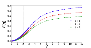
Figure 6: Truncation error for keeping first few (1-3) eigenvalues for embedding $D$. The truncation error for approximate embedding is less than $12\%$ in case of embedding in one dimension $E(q=1)$ up to $V\approx 1.5$ and for embedding in three dimension $E(q=3)$ up to $V\approx 2$.

Fig. (6) shows how the truncation error for retaining first few largest eigen values ($q=1-3$) behaves as a function of the interaction strength. As can be seen in the figure, the truncation error is less than $12\%$, for $q=1$ up to $V\approx 1.5$ and for $q=3$ up to $V\approx 2$.

V.2 Embedding with distortion

Another way of approximate embedding is the concept of embedding with distortion Indyk and Matousek (2004); Rabinovich (2003); Abraham et al. (2011). In general the method involves embedding the points in a low dimensional Euclidean space but with an error in the distance matrix. A measure of the distortion of the distance matrix, the average distortion, is defined as Rabinovich (2003); Abraham et al. (2011),

$$\epsilon_{avg}\equiv\frac{\sum_{i,j}D_{ij}}{\sum_{i,j}\tilde{D}_{ij}}$$ (39)

where $\tilde{D}_{ij}$ are the distances in the low dimensional Euclidean space. The low dimensional space is chosen such that the average distortion is minimized.

We implement this method as follows. We have a set of $L$ vectors in $L-1$ dimensions, $\{\mathbf{x_{i}}\}$ ($i=1,\dots,L$), $\mathbf{x_{i}}\in\mathbb{R}^{(L-1)}$, obtained from isometric Euclidean embedding as discussed in Section IV.4. We explore the $(L-1)C_{q}$, $q$ dimensional subspaces obtained by picking $q$ of the basis vectors, compute the average distortion for each case and pick the one that minimizes it. We label the above minimum value of average distortion as $\epsilon_{min}$. Note that our procedure is not optimal since we would probably get lower values of the average distortion by rotating each set of basis. So what we obtain are upper bounds on the average distortion.

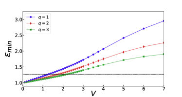
Figure 7: Average distortion for approximate embedding of $D$ in lower dimensions as a function of interaction strength.

Fig. (7) shows the average distortion as a function of interaction strength for $q=1,2,3$. Note that $\epsilon_{avg}=1$ corresponds to the case where there is no distortion. We find embedding with values of average distortion very close to the value one is possible for small values of interaction, $V\ll 2$. Corresponding to the upper bound of error $0.12$ in region $V\precsim 2$ we find the maximum average distortion allowed to be 1.27. For $V>2$, the average distortion is large and the truncation error for keeping three eigenvalues is high as well, so approximate Euclidean embedding of $D$ into lower dimensional subspaces is not possible.

VI Approximate embedding of the Wasserstein distance

In Section III.1, we had defined another distance function, $W(m_{i},m_{j})$, namely the Wasserstein distance or the transportation distance associated with two vertices of the graph. $W(m_{i},m_{j})$ is computed in terms of $D(i,j)$ and hence, in principle, contains no information about the state. However, as we detail in this section, the approximate embedding properties of the Wasserstein distance matrix seem to be more physically revealing than those of $D(i,j)$.

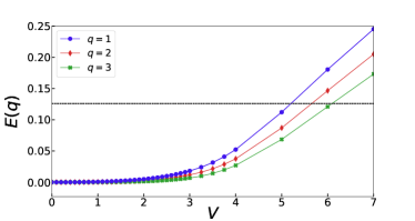
Figure 8: Truncation error for keeping first few $(1-3)$ eigenvalues of $G$ as a function of the interaction strength, for approximate embedding of $W$.

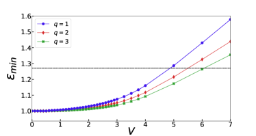
Figure 9: Average distortion for approximate embedding of $W$ as a function of the interaction strength.

In particular, we show that: (a) the embedding of $W(m_{i},m_{j})$ distinguishes between the metallic and insulating regimes more sharply than the embedding of $D(i,j)$. (b) $W(m_{i},m_{j})$ can be embedded in a finite dimensional Euclidean space with smaller error and average distortion than $D(i,j)$, for values of $V/t\gg 2$, namely well in the insulating regime.

Thus, $W(m_{i},m_{j})$ can be used to visualise the embedding in the metallic as well as insulating regimes. We illustrate this by presenting the “shapes” given by the vector configurations obtained by low average distortion in both these regimes.

VI.1 Approximate embedding of $W$ by truncation

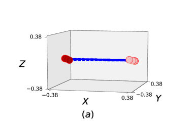
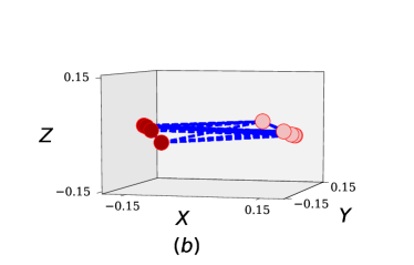
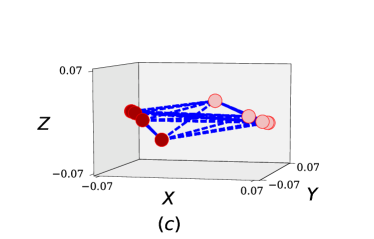
Figure 10: The embedded vectors of the Wasserstein distance in three dimensions. (a) $V=1$ with average distortion $<1\%$. (b) $V=3$ with $3\%$ average distortion and (c) $V=6$ with $27\%$ average distortion. Note that the scales of the axes are different in the three plots.

At $V=0$, both the distance matrices $D$ and $W$ are identical, thus the embedding gives two mirror points $k_{in}$ and $k_{out}$ in one-dimension (Section IV.3). Following the procedure of Section (V.1) we compute the truncation error for keeping first three eigenvalues of $G$. The results are plotted in Fig. (8). In the metallic regime, the error is extremely small even if only one eigenvalue is retained. The errors grow rapidly in the crossover regime and continue to grow in the insulating regime.

VI.2 Approximate embedding of $W$ by distortion

The average distortion for the embedding in one, two and three dimensions is plotted in Fig. (9). Again we see that the average distortion is almost negligible in the metallic regime and grows rapidly after $V\approx 3$. However, well into the insulating regime, up to around $V=6$, the distortion remains reasonably small, less than about $27\%$.

The above discussion shows that the Wasserstein distance matrix can be embedded in one dimension with negligible distortion in the metallic regime and in low dimensional Euclidean spaces well into the insulating regime with low distortion. Thus, it seems to capture the physics of the state in a clearer way than the distance matrix. It also seems to provide a way to visualise the many-body correlated state, both in the metallic and in the insulating regime.

In Fig. (10), we have plotted the embedded vectors for $V=1,3~{}{\rm and}~{}6$, for the three dimensional embedding. The filled circles represent $k_{in}$ and the unshaded circles represent $k_{out}$. Some points almost coincide and hence all the $18$ points cannot be seen distincly in the figure.

Fig. (10-a) plots the embedded points at $V=1$ (metallic regime) with very small ($<1\%$) average distortion. The two sets of points are clustered around $(x,y,z)=(\pm 0.35,0,0)$. The range of the spread in the $y$ and $z$ coordinates are $0.02$ and $0.03$ respectively. They are spread over a region less that $5\%$ of the range of the $x$ coordinate ($0.7$). Thus, set of embedded points, to a very good approximation, lie in a one dimensional subspace.

Fig. (10-b) plots the embedded points at $V=3$ (crossover regime) with $3\%$ average distortion. The points are all much closer to each other but the relative spread in the $y$ and $z$ directions have increased. The ranges of the spread in the $x,y~{}{\rm and~{}z}$ coordinates are now $0.36$, $0.05$ and  $0.06$ respectively. Thus the spreads in the $y$ and $z$ directions are now about $10\%$ of the spread in the $x$ direction.

The embedded points at $V=6$ with $27\%$ average distortion are plotted in Fig. (10-c). The ranges of the spread in the $x,y$ and $z$ coordinates are $0.13,0.04~{}{\rm and~{}}0.05$ respectively. The spreads in the $y$ and $z$ directions have now increased to $30\%$-$40\%$ of the spread in the $x$ direction.

The approximate embedding of the Wasserstein distances thus yields the following visualisation of the many-body state as a function of the interaction strength. In the metallic regime the embedding basically consist of two points. One representing all the points in the Fermi sea and the other all the points outside it. In the crossover regime, the distances between the points reduce and hence all the points come closer to each other. The one-dimensional nature is lost and the points spread out in the other two directions. This trend continues in the insulating regime.

VII Discussion and conclusion

To summarize our results, we have studied aspects of the intrinsic and extrinsic geometry of the ground state of a correlated system, by analysing its distance matrix on the Brillioun zone, defined in the previous work Hassan et al. (2018).

We have studied a system of interacting fermions on a finite size system. Hence we have used the mathematical methods of discrete geometry to analyse our results.

First we have studied the intrinsic curvature, as defined by Ollivier Ollivier (2009, 2010) and have shown that this quantity is distinctly different in the metallic and insulating regimes. The metallic regime is characterised by non-uniform curvatures while insulating regime is homogenous, characterised by uniform curvatures.

We have then studied the extrinsic geometry of the state by analysing the exact and approximate embedding of the distance matrix in Euclidean spaces. The exact embedding at extreme limits of interaction reveals for the metal at $V=0$, the distance matrix can be isometrically embedded in one dimension whereas for the CDW insulator at $V=\infty$, the isometric embedding of the distance matrix corresponds to an embedding dimension which scales as the system size and hence is not finite in the thermodynamic limit.

We showed that the distance matrix can be embedded in a finite dimensional Euclidean space with small error or average distortion in the metallic regime. This is not possible however in the insulating regime.

We find that the Wasserstein distance matrix constructed from the distance matrix, can be embedded in a one dimensional space in the metallic regime. Further, well within the insulating regime, it can be embedded in a finite dimensional Euclidean space with relatively small error and average distortion.

It is very appealing to be able to characterise a correlated many-body by a surface in a finite dimensional Euclidean space since we have a good feeling for Euclidean spaces. Our results indicate that while this is always possible for mean field states, the dimension of the embedding space for the correlated states may diverge as the system size, $L^{d}$. Since there are only $L^{d}$ embedded points, these will not form any smooth surface. Methods of approximate embedding seem to provide a method to obtain a smooth (though approximate) surface in a finite dimensional Euclidean space for correlated states. In particular, the Wasserstein distance matrix, defined in terms of the distance matrix seems to be more suited for this purpose rather than the distance matrix itself. We will be reporting on a more detailed analysis of this issue in a forthcoming paper.

VIII Acknowledgements

We are grateful to R. Simon, S. Ghosh, R. Anishetty, G. Date and Emil Saucan for useful discussions.

Appendix A Quantum distances of mean field states

In this section we generalise our previous results Hassan et al. (2018) of the distance matrix for mean field states (MFS).

We consider a general $d$-dimensional lattice with $L$ unit cells in each direction. We label the sites of the unit cells by $i$ and the sublattices by $a=1,\dots N_{B}$. The sites of the lattice are denoted by $\mathbf{R}_{ia}=\mathbf{R}_{i}+\mathbf{r}_{a}$. Thus $\mathbf{R}_{i}$ specifies a point in the unit cell and $\mathbf{r}_{a}$ the locations of the sub-lattice sites with respect to that point. The fermion creation and annihilation operators are denoted by $(C^{\dagger}_{ia},C_{ia})$. They satisfy the canonical anti-commutation relations. The Fourier transforms of these operators are defined as,

$$C_{a}(\mathbf{k})\equiv\frac{1}{L^{\frac{d}{2}}}\sum_{i}~{}e^{i\mathbf{k}\cdot\mathbf{R}_{ia}}C_{ia}$$ (40)

where $\mathbf{k}\in BZ$.

We denote the single-particle hamiltonian in the quasi-momentum space by $h_{ab}(\mathbf{k})$ and its spectrum by,

$$h_{ab}(\mathbf{k})u^{n}_{b}(\mathbf{k})=\epsilon^{n}(\mathbf{k})u^{n}_{a}(\mathbf{k}).$$ (41)

We denote the Fermi level by $\epsilon_{F}$ and the number of occupied bands at $\mathbf{k}$ by $N_{F}(\mathbf{k})$, namely,

$$N_{F}(\mathbf{k})\equiv\sum_{n=1}^{N_{B}}\Theta\left(\epsilon_{F}-\epsilon^{n}(\mathbf{k})\right).$$ (42)

The general mean field state is defined as

$$|u,\epsilon_{F}\rangle\equiv\prod_{\mathbf{k}}\prod_{n=1}^{N_{F}(\mathbf{k})}\left(u^{n}_{a}(\mathbf{k})C^{\dagger}_{a}(\mathbf{k})\right)|0\rangle$$ (43)

where $u$ denotes the full set of eigenstates, $u^{n}(\mathbf{k})$. We define $\Psi_{a_{1},\dots a_{N(\mathbf{k})}}(\mathbf{k})$ to be the antisymmetrised product of the $N_{F}(\mathbf{k})$ single particle wave functions, $u^{n}(\mathbf{k})$,

$$\Psi_{a_{1}\dots a_{N_{F}(\mathbf{k})}}(\mathbf{k})=\sum_{P}(-1)^{P}\prod_{l=1}^{N_{F}(\mathbf{k})}u^{n}(\mathbf{k})_{a_{P}(l)}$$ (44)

The general mean field state can be written in the factorised form,

$$|\Psi(\mathbf{k})\rangle \equiv \left(\sum_{a}\Psi_{a_{1}\dots a_{N_{F}(\mathbf{k})}}(\mathbf{k})\prod_{l=1}^{N_{F}(\mathbf{k})}C^{\dagger}_{a_{l}}(\mathbf{k})\right)|0\rangle_{\mathbf{k}}$$

$$|u,\epsilon_{F}\rangle = \prod_{\mathbf{k}}|\Psi(\mathbf{k})\rangle$$ (45)

where $\sum_{a}$ denotes the sum over all the ${}^{N_{B}}C_{N_{F}(\mathbf{k})}$ combinations of the the index $a$ and $\prod_{\mathbf{k}}$ denotes the direct product of the states defined at each point in the $BZ$.

Our definition of the quantum distance matrix is,

$$D^{2}(\mathbf{k}_{1},\mathbf{k}_{2})\equiv 1-|\langle u,\epsilon_{F}|E(\mathbf{k}_{1},\mathbf{k}_{2})|u,\epsilon_{F}\rangle|^{\alpha}$$ (46)

where $E(\mathbf{k}_{1},\mathbf{k}_{2})$ are the exchange operators. They are unitary operators and their action of the fermion creation operators is given by,

$$E(\mathbf{k}_{1},\mathbf{k}_{2})C^{\dagger}_{a}(\mathbf{k}_{1})E^{\dagger}(\mathbf{k}_{1},\mathbf{k}_{2}) = \pm C^{\dagger}_{a}(\mathbf{k}_{2})$$ (47)

$$E(\mathbf{k}_{1},\mathbf{k}_{2})C^{\dagger}_{a}(\mathbf{k}_{2})E^{\dagger}(\mathbf{k}_{1},\mathbf{k}_{2}) = \pm C^{\dagger}_{a}(\mathbf{k}_{1}).$$ (48)

The $\pm$ signs above depend on the ordering convention of the creation operators in the definition of the many-body states. While it is important to keep track of them for correlated states, as we will see below, due to the factorized form of MFS, the distances are independent of the signs.

The action of the exchange operator on the states is

$$E(\mathbf{k}_{1},\mathbf{k}_{2})|\psi(\mathbf{k}_{1})\rangle\otimes|\psi(\mathbf{k}_{2})\rangle = \pm\left(\sum_{aa^{\prime}}\Psi_{a_{1}\dots a_{N_{F}(\mathbf{k}_{1})}}(\mathbf{k}_{1})\right.$$

$$\left.\Psi_{a^{\prime}_{1}\dots a^{\prime}_{N_{F}(\mathbf{k}_{2})}}(\mathbf{k}_{2})\right)$$

$$\prod_{l^{\prime}=1}^{N_{F}(\mathbf{k}_{2})}C^{\dagger}_{a_{l}^{\prime}}(\mathbf{k}_{2})|0\rangle_{\mathbf{k}_{2}}$$

$$\otimes\prod_{l=1}^{N_{F}(\mathbf{k}_{1})}C^{\dagger}_{a_{l}}(\mathbf{k}_{1})|0\rangle_{\mathbf{k}_{1}}.$$

Equations (46), (47), (48) and (LABEL:eonstates) imply

$$D^{2}(\mathbf{k}_{1},\mathbf{k}_{2})=1-\left|\langle\Psi(\mathbf{k}_{1}))|\Psi(\mathbf{k}_{2}))\rangle\right|^{2\alpha}\delta_{N_{F}(\mathbf{k}_{1}),N_{F}(\mathbf{k}_{2})}.$$ (50)

Note that when $\alpha=1$, the RHS of the above equation is the Hilbert- Schmidt distance between $\Psi(\mathbf{k}_{1})$ and $\Psi(\mathbf{k}_{2})$. Thus we have shown that the quantum distances of the mean field states reduce to the standard definition in terms of the overlap of wavefunctions. For $\alpha=1$, it is exactly the Hilbert-Schmidt distance between the $N_{F(\mathbf{k})}$ states at $\mathbf{k}$. Our definition also implies that the distance between two quasi-momenta with different occupation numbers is equal to 1.

Appendix B Euclidean embedding of CDW states

In this section we implement the procedure described in section IV.2 and give an explicit solution to the problem of isometrically embedding the distance matrix of the CDW state in a Euclidean space.

Using the definitions, the matrix of the squared distances, $D_{CDW}^{2}$ can be written as Hassan et al. (2018):

$$D_{CDW}^{2}=\frac{3}{4}\left(\begin{array}[]{cc}{\cal I}-I&{\cal I}-I\\ {\cal I}-I&{\cal I}-I\end{array}\right)+\left(\begin{array}[]{cc}0&I\\ I&0\end{array}\right).$$ (51)

Note that $ee^{T}={\cal I}$, where $e$ is defined below equation(28). The Gram matrix defined in equation(28) is,

$$G_{CDW} = -\frac{1}{2}AD_{CDW}^{2}A$$ (52)

$$A \equiv \left(\begin{array}[]{cc}I&0\\ 0&I\end{array}\right)-\frac{1}{L}\left(\begin{array}[]{cc}{\cal I}&{\cal I}\\ {\cal I}&{\cal I}\end{array}\right).$$ (57)

It is easy to check that,

$$\left[A,D_{CDW}^{2}\right]=0~{}\Rightarrow~{}\left[A,G_{CDW}\right]=0$$ (58)

Thus, $A$ and $G_{CDW}$ have the same eigenvectors. It is quite easy to construct them. We give the answer below.

Define a complete, orthonormal set of $\frac{L}{2}$ dimensional column vectors $a^{\mu}$, $\mu=1...\frac{L}{2}$, where $a^{1}=\sqrt{\frac{2}{L}}(1,1,\dots,1)^{T}$. Further define a complete set of $L$ dimensional orthonormal vectors,

$$b^{i} \equiv \frac{1}{\sqrt{2}}\left(\begin{array}[]{c}a^{i}\\ a^{i}\end{array}\right),~{}~{}~{}~{}~{}~{}~{}i=1,\dots,\frac{L}{2}$$ (61)

$$\equiv \frac{1}{\sqrt{2}}\left(\begin{array}[]{c}a^{i-L/2}\\ -a^{i-L/2}\end{array}\right),~{}i=\frac{L}{2}+1,\dots,L.$$ (64)

It can be verified that,

$$G_{CDW}b^{1} = 0$$ (65)

$$G_{CDW}b^{i} = \frac{1}{4}b^{i},~{}i=2,\dots,\frac{L}{2}$$ (66)

$$= \frac{1}{2}b^{i},~{}i=\frac{L}{2}+1,\dots,L.$$ (67)

Thus,

$$\left(G_{CDW}\right)_{ij}=\sum_{k=2}^{L/2}\frac{1}{4}b^{k}_{i}b^{k}_{j}+\sum_{k=L/2+1}^{L}\frac{1}{2}b^{k}_{i}b^{k}_{j}.$$ (68)

The above equations and the procedure described in Section IV.2 gives the explicit solution for the embedding to be the $L$, $(L-1)$-dimensional vectors, $x_{i},~{}i=1,\dots,L$, with components, $\left(x_{i}\right)^{n},~{}n=1,\dots,L-1$, given by

$$\left(x_{i}\right)^{n} = \frac{1}{2}b^{n+1}_{i},~{}~{}~{}~{}n=1,\dots,\frac{L}{2}-1$$ (69)

$$= \frac{1}{\sqrt{2}}b^{n+1}_{i},~{}~{}n=\frac{L}{2},\dots,(L-1).$$ (70)

Thus, the distance matrix at $V=\infty$, can be isometrically embedded in a Eulcidean space with dimension equal to $L-1$.

References

- Resta and Sorella (1999) R. Resta and S. Sorella, Phys. Rev. Lett. 82, 370 (1999).
- Resta (2002) R. Resta, Journal of Physics: Condensed Matter 14, R625 (2002).
- Haldane (2004) F. D. M. Haldane, Phys. Rev. Lett. 93, 206602 (2004).
- Landau (1937) L. D. Landau, Zh. Eksp. Teor. Fiz. 7, 19 (1937), [Ukr. J. Phys.53,25(2008)].
- Kohn (1964) W. Kohn, Phys. Rev. 133, A171 (1964).
- Aligia and Ortiz (1999) A. A. Aligia and G. Ortiz, Phys. Rev. Lett. 82, 2560 (1999).
- Resta (2011) R. Resta, The European Physical Journal B 79, 121 (2011).
- Souza et al. (2000) I. Souza, T. Wilkens, and R. M. Martin, Phys. Rev. B 62, 1666 (2000).
- Sgiarovello et al. (2001) C. Sgiarovello, M. Peressi, and R. Resta, Phys. Rev. B 64, 115202 (2001).
- Hassan et al. (2018) S. R. Hassan, R. Shankar, and A. Chakrabarti, Manuscript accepted and to be published in Phys. Rev. B. (2018).
- Yang and Yang (1966) C. N. Yang and C. P. Yang, Phys. Rev. 150, 321 (1966).
- Baxter (1982) R. J. Baxter, Exactly Solved Models in Statistical Mechanics (Academic Press, 1982).
- Cazalilla et al. (2011) M. A. Cazalilla, R. Citro, T. Giamarchi, E. Orignac, and M. Rigol, Rev. Mod. Phys. 83, 1405 (2011).
- Shankar (1990) R. Shankar, International Journal of Modern Physics B 04, 2371 (1990).
- Saucan and Appleboim (2009) E. Saucan and E. Appleboim, Mathematics of Surfaces XIII, edited by E. R. Hancock, R. R. Martin, and M. A. Sabin (Springer Berlin Heidelberg, Berlin, Heidelberg, 2009) pp. 335–355.
- Forman (2003) R. Forman, Discrete and Computational Geometry 29, 323 (2003).
- Ollivier (2009) Y. Ollivier, Journal of Functional Analysis 256, 810 (2009).
- Ollivier (2010) Y. Ollivier, Probabilistic Approach to Geometry, Vol. 57 (Mathematical Society of Japan, 2010).
- Lin et al. (2011) Y. Lin, L. Lu, and S.-T. Yau, Tohoku Math. J. (2) 63, 605 (2011).
- Ollivier (2013) Y. Ollivier, Analysis and Geometry of Metric Measure Spaces: Lecture Notes of the 50th Séminaire de Mathématiques Supérieures (SMS), Montréal, 2011, edited by A. S. Galia Dafni, Robert McCann (AMS, 2013) pp. 197–219.
- Villani (2008) C. Villani, Optimal Transport: Old and New, 2009th ed., Grundlehren der mathematischen Wissenschaften (Springer, 2008).
- Jost and Liu (2014) J. Jost and S. Liu, Discrete Comput. Geom. 51, 300 (2014).
- Loisel and Romon (2014) B. Loisel and P. Romon, Axioms 3, 119 (2014).
- Schoenberg (1937) I. J. Schoenberg, Annals of Mathematics 38, 787 (1937).
- Liberti and Lavor (2015) L. Liberti and C. Lavor, International Transactions in Operational Research 23 (2015), 10.1111/itor.12170.
- Dokmanic et al. (2015) I. Dokmanic, R. Parhizkar, J. Ranieri, and M. Vetterli, CoRR abs/1502.07541 (2015), arXiv:1502.07541 .
- Skillicorn (2008) D. B. Skillicorn, Understanding Complex Datasets: Data Mining with Matrix Decompositions (CRC press, 2008) pp. 49–87.
- Indyk and Matousek (2004) P. Indyk and J. Matousek, in Handbook of Discrete and Computational Geometry (CRC Press, 2004) pp. 177–196.
- Rabinovich (2003) Y. Rabinovich, Proceedings of the Thirty-fifth Annual ACM Symposium on Theory of Computing, STOC ’03, 456 (2003).
- Abraham et al. (2011) I. Abraham, Y. Bartal, and O. Neiman, Advances in Mathematics 228, 3026 (2011).