New Near-Infrared $JHK_{s}$ light-curve templates for RR Lyrae variables

We provide homogeneous optical ($UBVRI$) and near-infrared ($JHK$) time series photometry for 254 cluster ($\omega$ Cen, M4) and field RR Lyrae (RRL) variables. We ended up with more than 551,000 measurements and only a minor fraction (9%) were collected in the literature. For 94 fundamental (RRab) and 51 first overtones (RRc) we provide a complete optical/NIR characterization (mean magnitudes, luminosity amplitudes, epoch of the anchor point). The NIR light curves of these variables were adopted to provide new and accurate light-curve templates for both RRc (single period bin) and RRab (three period bins) variables. The templates for the $J$ and the $H$ band are newly introduced, together with the use of the pulsation period to discriminate among the different RRab templates. To overcome subtle uncertainties in the fit of secondary features of the light curves (dips, bumps) we provide two independent sets of analytical functions (Fourier series, Periodic Gaussian functions). The new templates were validated by using 26 $\omega$ Cen and Bulge RRLs covering the four period bins. We found that the difference between the measured mean magnitude along the light curve and the mean magnitude estimated by using the template on a single randomly extracted phase point is better than 0.01 mag ($\sigma$=0.04 mag). We also validated the template on variables for which at least three phase points were available, but without information on the phase of the anchor point. We found that the accuracy of the mean magnitudes is also $\sim$0.01 mag ($\sigma$=0.04 mag). The new templates were applied to the Large Magellanic Cloud (LMC) globular Reticulum and by using literature data and predicted PLZ relations we found true distance moduli of 18.47$\pm$0.10$\pm$0.03 mag ($J$) and 18.49$\pm$0.09$\pm$0.05 mag ($K$). We also used literature optical and mid-infrared data and we found a mean true distance modulus of 18.47$\pm$0.02$\pm$0.06 mag, suggesting that Reticulum is $\sim$1 kpc closer than the LMC.

1 Introduction

RR Lyrae (RRLs), are very accurate distance indicators and solid tracers of old (age ¿ 10 Gyr) stellar populations. The near-infrared (NIR) Period-Luminosity (PL) relations of RRLs will be the first calibrator of the extragalactic distance scale based on population II stars (Beaton et al. 2016), which will provide an independent estimate of $H_{0}$. The NIR bands, when compared with the optical bands, present several advantages. These become even more compelling for variable stars, like RRLs. It is therefore mandatory to fully exploit the advantages that the NIR bands bring up. They are the following.

i) The NIR bands are less prone to uncertainties in reddening corrections and are less affected by the occurrence of differential reddening. Indeed, the $K$ band is one order of magnitude less affected than the visual band. For this reason, the highly reddened regions of the Galactic center and of the inner bulge can only be investigated effectively in NIR bands. At these Galactic latitudes, the absorption in the $K$ band becomes of the order of 2.5-3.0 mag (Gonzalez et al. 2012), meaning $\sim$25-30 mag in the $V$ band. This is well beyond the capabilities of current and near-future optical observing facilities.

ii) The luminosity variation in the optical bands is dominated by variations in effective temperature, while in the NIR bands it is dominated by variations in stellar radius (Madore et al. 2013). This means that the NIR light curves are minimally affected by nonlinear phenomena like shock formation and propagation, which cause the appearance of either bumps and/or dips along the light curves. Moreover, the luminosity amplitudes steadily decrease when moving from the optical to the NIR bands and approach an almost constant value for wavelengths equal or longer than 2.2 $\mu$m (Madore et al. 2013). Indeed, the ratio in luminosity amplitudes $A_{Ks}/A_{V}$ and $A_{[3.6]}/A_{V}$ attain values ranging from 0.22 to 0.41 (RRc and RRab, respectively, Braga et al. 2018) and from 0.18 to 0.22 (RRc and RRab, respectively, Neeley et al. 2015).

iii) The typical sawtooth shape of the light curves of RRab in the optical is less sharp in the NIR, where light curves become more symmetrical. This means that, even with a modest number of phase points, the light curve can be well fitted.

The NIR bands, together with these “intrinsic advantages” also bring up several “extrinsic advantages” concerning the RRL distance scale.

i) Solid theoretical (Bono et al. 2001; Marconi et al. 2015) and empirical (Longmore et al. 1986; Bono et al. 2003) evidence indicates that RRLs obey well-defined Period-Luminosity-Metallicity (PLZ) relations in the NIR bands. The slope of the relation becomes steeper and its standard deviation decreases when moving toward longer wavelengths. The RRLs in the optical bands also obey mean Magnitude-Metallicity (MZ, Sandage 1981a, b) relations, but these are affected by non-linearity and evolutionary effects, and are less precise than the PLZ relations in the NIR bands (Caputo et al. 2000).

ii) In the case that both optical and NIR bands are available, one can adopt the newly developed algorithm REDIME (Bono et al. 2018). REDIME is capable of providing homogeneous and simultaneous estimates of metal content, distance and reddening.

However, the NIR bands also bring up some cons.

i) The identification and the characterization of RRLs is more difficult in the NIR bands, due to the decrease in luminosity amplitude and the less characteristic shape of the light curve, when moving from shorter- to longer-period variables.

ii) Accurate and deep NIR photometry is never trivial, in particular in crowded stellar fields. NIR observations are quite demanding of telescope time, since specific observing strategies must be devised to properly subtract the sky background. This means that NIR observations typically have shallower limiting magnitudes and longer observing runs when compared with optical bands. A practical example of this disadvantage is the comparison between the OGLE and VVV surveys in the Bulge. While the first covers a larger sky area and provides time series with thousands of phase points, the second achieved $\sim$100 phase point per time series in a smaller area, although being much more capable of piercing the dust in the Galactic plane. A very interesting and promising approach to overcome several of the limitations affecting the NIR bands is to use observing facilities that are assisted by an adaptive optics system. However, these complex detectors have a quite limited field of view, typically of the order of one arcminute or even smaller. This means that they can hardly be adopted for a photometric survey and/or for an efficient detection and characterization of variable stars.

iii) To overcome possible nonlinear effects in cameras and/or the saturation of bright stars, and to improve sky subtraction, the NIR images are collected as series of short-exposure images, arranged in specific dithering pattern. Several approaches have been suggested in the literature to perform PSF photometry of NIR images and all of them present pros and cons.

These limitations of NIR photometry are at the base of the development of NIR light curve template. More than twenty years ago, Jones et al. (1996, henceforth, J96) provided, in a seminal investigation, the first NIR light-curve templates for RRLs. What really matters in this context is that—once the period of an RRL is already known, preferentially from optical data, together with its optical amplitude and its epoch of maximum light—a template provides the opportunity to estimate its mean $K$-band magnitude on the basis of a single NIR measurement. However, the J96 templates were provided only for the $K$-band. Furthermore, owing to the limited number of NIR measurements available at that time it was only based on 17 RRab and 4 RRc. J96 divided RRab variables into four subgroups and kept the RRc variables within a single group, therefore obtaining four and one light-curves template, respectively. However, the bins in luminosity amplitude adopted to split the fundamental pulsators into different sub-groups did not overlap one another (see Fig. 1). It is also worth mentioning that the use of the luminosity amplitude to discriminate RRLs with different shapes of the light curve might also be affected by degeneracy. Indeed, the Bailey diagram (luminosity amplitude versus period) shows that the trend of both RRc and RRab luminosity amplitudes is not linear over their typical period range (Cacciari et al. 2005; Kunder et al. 2013). This means that two variables that have the same amplitude might have different periods.

To overcome some of these intrinsic limitations of the J96 NIR light-curve templates, new approaches have been recently proposed in the literature. It has been suggested by Freedman & Madore (2010) that accurate optical bands for Classical Cepheids can be transformed into the NIR bands using only a few measurements. The same approach was also applied to RRLs by Beaton et al. (2016), the experiment was limited to a single RRL as a preliminary result of their ongoing investigation based on $HST$ data. The key advantage of this method is that it does not require knowledge of the epoch of maximum light to phase the NIR measurements. More recently, (Hajdu et al. 2018) suggested an interesting new method to use a well-sampled $K_{s}$-band light curve to estimate the $J$- and the $H$-band mean magnitude of an RRL from single-epoch measurements. They used data from the VISTA Variables in the Vía Láctea (VVV) survey and decomposed the $K_{s}$-band light curves of 101 RRab variables into orthogonal Principal Components. Their method also provides estimates of photometric metallicities.

Light-curve templates of RRLs have also been developed in the visual bands. Layden (1998) obtained six $V$-band light-curve templates, but they were limited to RRab variables. The adopted sample of 103 field RRLs was divided according to the shape of the light curve (Bailey types $a$ and $b$, plus the phase range of the rising branch). They were used to estimate simultaneously mean magnitude and luminosity amplitude. More recently, optical ($ugriz$) light-curve templates of RRLs were derived by Sesar et al. (2010) from SDSS photometry of 379 RRab and 104 RRc. They provided 22 RRab templates and two RRc templates for the five $ugriz$ SDSS bands. They found evidence that the shape of the RRab light curves steadily changes when moving from the blue to the red edge of the instability strip, while RRc light curves are dichotomous. They claim that this evidence might suggest the possible occurrence of second-overtone RRLs. However, theoretical models and spectroscopic measurements indicate that shorter period RRc variables are, on average, more metal-rich than the bulk of field RRc variables (Bono et al. 1997; Sneden et al. 2017), providing an alternative explanation to the hypothesis of second overtone RRLs. In passing, it is worth mentioning that the light-curve templates by Sesar et al. (2010) were mainly developed for RRL identification—especially within the upcoming LSST survey—rather than to determine their mean magnitudes.

The main aim of this investigation is to provide new NIR light-curve templates for RRLs based on a detailed optical and NIR data set that our group collected for RRLs in the Galactic Globular Clusters (GGC) $\omega$ Cen and M4, supplemented by literature photoelectric photometry of Milky Way RRLs.

The structure of the paper is as follows. In Section 2, we describe the optical and the NIR photometric data sets adopted for the current analysis. In §˜3 we deal with the NIR light-curve templates and, in particular, with the criteria adopted to select the period bins and the normalization of the light curves. The analytical form of the light-curve templates are discussed in Section 3.2 together with a detailed discussion of the adopted anchor point to phase NIR measurements. Section 5 is dedicated to the validation of the templates. The validation is based on $\omega$ Cen data and OGLE+VVV (Udalski et al. 1992; Minniti et al. 2010) data and it was performed for single and triple phase points. In Section 6 we apply the new NIR templates to the $J$ and $K_{s}$ light curves of RRLs in the extragalactic GC Reticulum and provide a new true distance modulus determination. We summarize our results in Section 7 and briefly outline future developments of the current project.

2 Optical and near-infrared data sets

We use proprietary—still unpublished until this work—optical and NIR PSF-reduced photometry of RRLs in M4 (Stetson et al. 2014) and in $\omega$ Cen (Braga et al. 2016, 2018). Optical data are in the (Landolt 1983, 1992) system, and NIR data are in the 2MASS photometric system (Skrutskie et al. 2006). Note that the NIR data were binned by epoch, therefore each phase point is actually an average of three to five phase points belonging to the same dithering sequence. The binning process is described in detail in Braga et al. (2018). More insights on the data (telescopes, cameras, and reduction) can be found in Stetson et al. (2014), Braga et al. (2016) and Braga et al. (2018).

These data were supplemented with i) relatively old optical and NIR photoelectric photometry of 26 Milky Way (MW) field RRLs, mostly collected to perform Baade-Wesselink (BW) analysis (Carney & Latham 1984; Cacciari et al. 1987; Jones et al. 1987; Barnes et al. 1988; Jones et al. 1988a, b; Liu & Janes 1989; Skillen et al. 1989; Clementini et al. 1990; Fernley et al. 1990; Barnes et al. 1992; Cacciari et al. 1992; Jones et al. 1992; Skillen et al. 1993a, b), which we call the “BW” sample, and ii) optical data from long-term photometric surveys (ASAS: Pojmanski 1997; NSVS: Woźniak et al. 2004). Note that the photoelectric data were not available in machine-readable format, therefore we have digitized the tables available in the original papers. Moreover, to deal with a homogeneous data set, we transformed all the photoelectric NIR data to the 2MASS system. We have used the transformations by Carpenter (2001) to convert the magnitudes from the CIT system (Jones et al. 1987; Liu & Janes 1989; Jones et al. 1988a, b; Barnes et al. 1992; Jones et al. 1992), UKIRT system (Skillen et al. 1989), SAAO system (Fernley et al. 1990; Skillen et al. 1993a) and ESO system (Cacciari et al. 1992) to the 2MASS system. Note that more recent transformations between the SAAO and 2MASS system are available (Koen et al. 2007). However, these would require measurements in the $H$-band which are not available for the Fernley et al. (1990) data. On the other hand, the optical photoelectric data are all in the Johnson system. However, we only use these optical data to derive the epoch of the mean magnitude on the rising branch ($t_{ris}$), independently for each variable. Therefore, they were not homogenized with the CCD data in the Landolt system.

The key advantage of $\omega$ Cen RRLs is that this stellar system contains almost 200 RRLs and they cover a range in metal content of at least one dex (Rey et al. 2000; Sollima et al. 2006). Moreover, it is the only cluster—with the exception of the peculiar metal-rich clusters NGC 6388 (Pritzl et al. 2002) and NGC 6441 (Pritzl et al. 2001)—hosting a sizable sample of long-period (P$>$0.7 days) RRLs.

To make a homogeneous Optical and NIR data set available to the entire astronomical community, Table 2 and Table 3 give, respectively, the $UBVRI$ and $JHK_{s}$ light curves of 233 RRLs in $\omega$ Cen and M4; Table 3, also provides $JHK_{s}$ light curves for 21 RRLs in the BW sample. Table 2 is based on the optical data collected during $\sim$20-year-long campaigns (Stetson et al. 2014; Braga et al. 2016) and are calibrated to the Landolt ($UBV$) and Kron-Cousins ($RI$) photometric system. Note that Table 2 contains also literature data (Sturch 1978; Kaluzny et al. 1997, 2004 plus the CATALINA Drake et al. 2009 and ASAS-SN surveys Shappee et al. 2014; Kochanek et al. 2017) which we used to supplement our photometry (more details in Section 3.1 of Braga et al. 2016). Table 3 includes objects for which either we collected NIR time series data during 10-year-long observation campaigns (Stetson et al. 2014; Braga et al. 2018) or NIR photometry was available in the literature. NIR measurmenets listed in Table 3 are in the 2MASS photometric system. Note that the fraction of objects adopted for the NIR light-curve templates is 57% of the total number of objects listed in Table 3.

Table 1: $UBVRI$ light curves of $\omega$ Cen and M4 RRLs.

Name	band	HJD–2,400,000	mag	err	dataset		days	mag	mag
$\omega$Cen-V3	1	54705.4699	14.950	0.005	B19
$\omega$Cen-V3	1	50601.5756	14.767	0.022	B19
$\omega$Cen-V3	1	50601.5802	14.775	0.022	B19
$\omega$Cen-V3	1	50920.7741	15.335	0.017	B19
$\omega$Cen-V3	1	53795.8733	14.428	0.039	B19
$\omega$Cen-V3	1	53795.8858	14.487	0.065	B19
$\omega$Cen-V3	1	51368.4851	15.320	0.003	B19
$\omega$Cen-V3	1	51369.4884	15.339	0.003	B19
$\omega$Cen-V3	1	52443.4731	15.245	0.011	B19
$\omega$Cen-V3	1	52443.4773	15.223	0.011	B19

Table 2: $JHK_{s}$ light curves of $\omega$ Cen, M4 and BW RRLs.

Name	Flag	band	HJD–2,400,000	mag	err
			days	mag	mag
$\omega$Cen-V3		1	55341.5764	13.137	0.006
$\omega$Cen-V3		1	55341.5878	13.147	0.007
$\omega$Cen-V3		1	55341.6006	13.175	0.004
$\omega$Cen-V3		1	55341.6074	13.179	0.013
$\omega$Cen-V3		1	51946.8638	13.053	0.013
$\omega$Cen-V3		1	51948.7440	13.154	0.012
$\omega$Cen-V3		1	51948.8136	13.170	0.008
$\omega$Cen-V3		1	52308.7494	13.075	0.013
$\omega$Cen-V3		1	52308.8255	13.117	0.016
$\omega$Cen-V3		1	52308.8674	13.145	0.011

2.1 Sample selection

To derive accurate and precise NIR light-curve templates we selected from the initial RRL sample the variables satisfying the following criteria.

1) — At least 10 phase points in $J$, $H$ or $K_{s}$.

2) — An accurate estimate of $t_{ris}$ (see Appendix 7 for the calculation of $t_{ris}$), i.e., the epoch to which the template is anchored.

3) — A small dispersion ($\sigma\lesssim$0.1) of the phase points along the normalized light curve. To derive the light-curve templates, all the light curves were divided by their amplitude (see Section 4). The variables with limited photometric accuracy are more likely to increase the dispersion of the normalized light curve, and in turn of the light curve template. Our approach was conservative: we only included variables with a “clean” trend in the normalized light-curve fit.

4) — Special care was taken to include variables that trace the shape of the light curve of both RRab and RRc when moving from shorter to longer period RRLs. This means the occurrence of either dips just before the phase of maximum light and/or bumps just before the phase of minimum light.

Once we apply these selection criteria we are left with a subsample of 94 RRab and 51 RRc variables. The excluded variables are marked with an asterisk in Table 3. In the following, the selected objects, belonging to $\omega$ Cen, to M4, or to the BW sample are called “Template Data Sample” (TDS);their pulsation properties are listed in Table LABEL:tab:sample. The reader interested in a more detailed discussion of the approach adopted to derive periods, mean magnitudes, amplitudes and their uncertainties is referred to Stetson et al. (2014), Braga et al. (2016) and Braga et al. (2018). The photometric properties of field RRLs were derived using the PLOESS polynomial fit (Braga et al. 2018). Note that the number of variables with accurate light curves in all three filters is limited. More specifically, the light-curve templates rely on a number of variables ranging from 142 for the $J$ band to 101 for the $H$ band and 112 for the $K_{s}$ band. The difference among the three bands is mainly caused by the paucity of $H$-band data for field and M4 RRLs. Moreover, the $H$- and $K_{s}$-band light curves have luminosity amplitudes that are half the $J$-band amplitudes. This means that the photometric scatter in the normalized light curves appears larger.

3 Near-Infrared light curve templates

3.1 Selection of the period bins

We defined the template bins according to the pulsation period of the variable. The reasons are manifold. i) – The period is a solid observable, since it can be firmly estimated also for variables showing multi-periodicity (Blazhko, mixed-mode). The same statement does not apply to the luminosity amplitude adopted by J96. ii) – The period range covered by TDS variables (0.28-0.47 days for RRcs and 0.39-0.87 days for RRabs) is much larger than the RRL sample adopted by J96 (0.25-0.34 days for RRc and 0.39-0.66 days for RRabs). iii) – The optical luminosity amplitude is not a linear function of the period (Cacciari et al. 2005; Kunder et al. 2013). Data plotted in the Bailey diagram (logarithmic period versus luminosity amplitudes, Fig. 1) clearly show that RRab and RRc variables with similar amplitudes can have significantly different pulsation periods. iv) – The period is tightly correlated with the intrinsic parameters (stellar mass, luminosity, effective temperature) of the variable (Bono & Stellingwerf 1994).

We have checked that, for RRc variables, one template bin is enough because the shape of the light curve in the NIR bands is almost sinusoidal over the whole period range. On the other hand, the RRab variables were divided into three period bins for following reasons. i) – To improve the sampling along the light curve template we required at least ten variables per bin for each band, limiting the number of possible period bins. ii) – The RRab variables display in the optical Bailey diagram a parabolic trend (Cacciari et al. 2005) when moving from shorter to longer periods. Data plotted in Fig. 1 show that the maximum is located at approximately 0.55 days. iii) – We also decided to cut the sample at 0.7 days, because empirical evidence indicates that a transition—both in Blazhko properties and in the optical-to-NIR amplitude ratios—takes place across this boundary (Prudil & Skarka 2017; Braga et al. 2018).

This means that the RRab variables were split into short (RRab1, P$\leq$0.55 days), medium (RRab2, 0.55$<$P$<$0.70 days) and long (RRab3, P$\geq 0.70$ days) period bins, while the RRc constitute a single period bin (0.28$<$P$<$0.47 days).

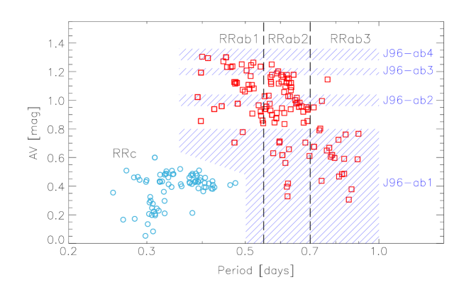
Figure 1: Bailey diagram, $V$-band amplitude versus logarithmic period, for $\omega$ Cen RRLs. Blue circles mark RRc variables, while red squares mark RRab variables. The ranges in period for the RRab light-curve templates are indicated by vertical black dashed lines. The blue striped areas show the ranges in amplitude adopted for the light curve templates by J96. Note that they provided thresholds in the $B$ band, but here they have been rescaled by 1.25, i.e., the typical amplitude ratio ($AB/AV$) for RRab variables (Braga et al. 2016).

It is worth mentioning that we could have extended the period range of the RRab3 template up to 0.9 days, by including $\omega$Cen-V91 and $\omega$Cen-V150. However, both variables have light curves with a significantly different shape when compared to the other RRLs in RRab3 sub-sample. More statistics are required to establish whether RRLs with periods longer than $\sim$0.87 days require a separated template bin.

Finally we mention that the number of phase points per template bin is 1,226 ($J$), 698 ($H$), 959 ($K_{s}$) for the RRc template; 931 ($J$), 478 ($H$), 1,125 ($K_{s}$) for the RRab1 template; 1,662 ($J$), 995 ($H$), 1,709 ($K_{s}$) for the RRab2 template; 440 ($J$), 284 ($H$), 512 ($K_{s}$) for the RRab3 template. The current data set is more than six times larger than the data set adopted by J96, and more than 2.5 times larger, if considering only the $K-s$-band data.

3.2 Normalization of the light curves

The NIR light-curve templates we are developing provide the mean magnitude $\langle X\rangle$ of an RRL with an accuracy of the order of a few hundredths of a magnitude provided that the following data are available:

i) the epoch ($t$) and the magnitude ($X_{t}$) of a phase point;

ii) the period of the variable ($P$);

iii) the luminosity amplitude in either the $V$ or $B$ band ($AV$ or $AB$);

iv) the epoch of the anchor point along the light curve. In this investigation, we adopt the epoch of the mean magnitude on the rising branch ($t_{ris}$). It was already demonstrated by (Inno et al. 2015) that for Classical Cepheids (CCs), $t_{ris}$ is a more precise anchor point than the more commonly-used epoch of the maximum light ($t_{max}$).

We performed a number of simulations using optical and NIR light curves for which both $t_{ris}$ and $t_{max}$ were available and we found that the former is better defined when moving from the blue to the red edge of the RRL instability strip. The reasons why $t_{ris}$ is better defined than $t_{max}$ are twofold. i) Large-amplitude RRab variables characterized by a “sawtooth” light curve show a cuspy maximum. This means that the phases across maximum light occur during a short time range, so an accurate estimate of the epoch of maximum light requires high time resolution. ii) Some RRc variables display a well-defined dip just before maximum light (U Com, Bono et al. 2000). To properly identify and separate the two maxima, high time resolution is also required for these short-period variables.

The mean NIR magnitude, $\langle X\rangle$, of a variable for which the aforementioned parameters are available can be estimated by using the following relation:

$$\langle X\rangle=X_{t}-AX\cdot T({\phi}_{t})$$ (1)

where ${\phi}_{t}=\dfrac{t-t_{ris}}{P}$ is the difference in phase between the NIR phase point that was observed and the epoch, $t_{ris}$, of the anchor point, while $AX$ is the luminosity amplitude in the $X$ band. Note that the latter is typically unknown, but it can be estimated from the optical amplitude and empirical NIR-over-optical amplitude ratios (Braga et al. 2018). Note also that the light-curve templates must be normalized.

To generate the normalized light-curve templates, we adopted the magnitudes $m_{ijk}$ of the TDS variables, marked with an asterisk in Table 3 and listed in Table LABEL:tab:sample, where $i$ indicates the $i$-th phase point of the empirical light curve, $j$ indicates the band (1 for $J$, 2 for $H$ and 3 for $K_{s}$), and $k$ indicates the $k$-th RRL in the TDS sample. We have transformed all the empirical $m_{ijk}$ measurements into normalized magnitudes $M_{ijk}$ by subtracting from each $k$-th RRL its mean magnitude in the $j$-th band (see Table LABEL:tab:sample $\langle m_{jk}\rangle$) and by dividing for the $j$-th band amplitude (see Table LABEL:tab:sample $A_{jk}$) according to the following relation: $M_{ijk}=\dfrac{m_{ijk}-\langle m_{jk}\rangle}{A_{jk}}$. Fig. 2 and 3 show the final normalized light curves as a function of the pulsation phase for the TDS sample.

4 Analytical fits to the light curve templates

Once the normalized light curves for the three NIR bands and for the different period bins have been fixed we performed an analytical fit of the light curve templates. We adopted two different fitting functions: Fourier series (Section 4.1) and periodic Gaussians (PEGASUS, Section 4.2).

4.1 Fourier fit

We have fit the normalized light curves with Fourier series of the $i$-th order

$$F(\phi)=A_{0}+\Sigma_{i}A_{i}\cos{(2\pi i\phi-\phi_{i})}$$ (2)

with $i$ ranging from two to seven. The red lines plotted in the left panels of Fig. 2 show the individual fits for the three different bands and for the four light-curve templates.

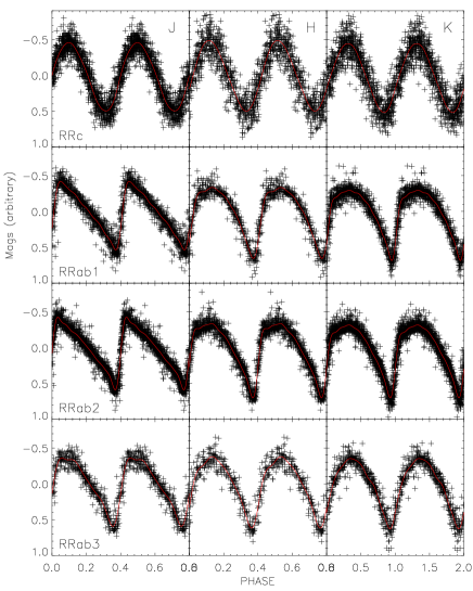
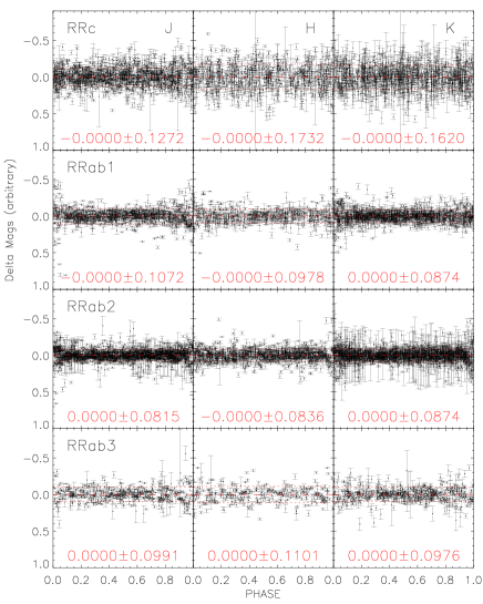
Figure 2: Left panels: from left to right the different panels display the Fourier fits of the normalized $JHK_{s}$ light curves. From top to bottom the panels show the four (RRc, RRab1, RRab2, RRab3) different ranges in period. Right panels: Same as the left, but for the residuals of the normalized light curves with the Fourier fits. The median and standard deviation of the median are labelled in red.

It is noteworthy that the agreement between the analytical fits and observations is, within the errors, quite good over the entire pulsation cycle. In particular, the fits properly represent the data across the phases of minimum light in which the variation of the luminosity is more cuspy. Interestingly enough, we found that the residuals between the normalized light curves and the Fourier fits plotted in the right panels of the same figure are vanishing. They are typically smaller than the fourth decimal place. Moreover and even more importantly, the residuals do not show any phase dependence within the standard deviation (dashed red lines) of the analytical fits. In this context it is worth mentioning that the light-curve templates derived by J96 were obtained using 2^nd-order Fourier fits for the RRc variables and 6^th-order Fourier fits for the RRab variables. We used different orders for almost all the period bins, however, we adopted the 6^th order for the fit of the RRab3 $K_{s}$-band templates. This template includes roughly the same number of variables as the RRab1 template by J96 ($AB<$1.0 mag), however the coefficients of the fit are significantly different.

4.2 PEGASUS fit

We also performed an independent fit of the normalized light curves using a series of periodic Gaussians, presented in Inno et al. (2015) with $i$ ranging from two to six.

$$P(\phi)=A_{0}+\Sigma_{i}A_{i}\exp{\Big{(}-\sin{\Big{(}\dfrac{\pi(\phi-\phi_{i})}{\sigma_{i}}\Big{)}^{2}}\Big{)}}$$ (3)

Data plotted in the left panels of Fig. 3 show that PEGASUS fits follow the variation of the normalized light curves quite well over the entire pulsation cycle. This applies not only to the RRc, but also to the RRab light-curve templates. The main difference between the fits based either on PEGASUS or on Fourier series is that the former display a smoother variation over the entire pulsation cycle, while the latter show several small bumps/ripples. The NIR light curves with accurate photometry and very well sampled light curves do not display these bumps. This suggests that the bumps/ripples are spurious variations of the order of a few thousandths of a magnitude among the different variables included in a given period bin.

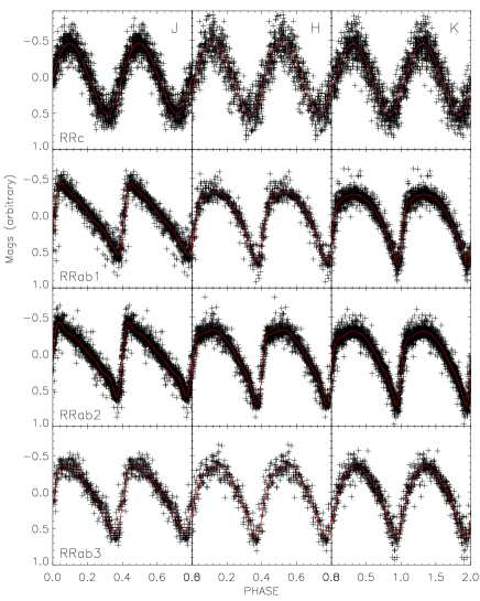
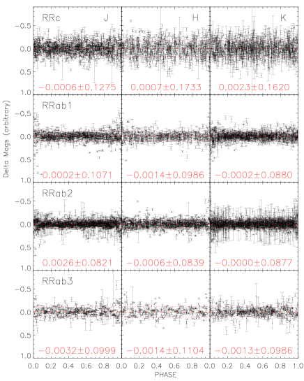
Figure 3: Left panels: from left to right the different panels display the PEGASUS fits of the normalized $JHK_{s}$ light curves. From top to bottom the panels show the four (RRc, RRab1, RRab2, RRab3) different ranges in period. Right panels: Same as the left, but for the residuals of the normalized light curves with the PEGASUS fits. The median and standard deviation of the median are labelled in red.

The residuals between the normalized light curves and the PEGASUS fits are plotted in the right panels of the same figure. They are of the order of a few thousandths, i.e., slightly larger than the residuals of the Fourier fits. The difference is mainly due to the smoothness of the PEGASUS fits compared with the Fourier fits.

4.2.1 Phases of minimum and maximum along the light curve template

Although there are solid reasons supporting the idea that $t_{ris}$ is easier to derive than the epoch of maximum light, $t_{max}$, and it provides a more precise epoch of reference, we are aware that all the recent surveys adopted $t_{max}$ as the reference epoch for RRLs and other variable stars. For this reason we also provide the phases of both minimum and maximum (${\phi}_{max}$ and ${\phi}_{min}$) of the current light-curve templates (see Table 4). These pulsation phases—which can be considered typical—provide the opportunity to use the current templates to estimate the mean magnitude of variables for which only $t_{max}$ and/or $t_{min}$ is available in the literature.

Table 3: Phases of minimum and maximum of the light curves templates.

Template	band	$\phi_{min(F)}$	$\phi_{max(F)}$	$\phi_{min(P)}$	$\phi_{max(P)}$
RRc	$J$	0.785	0.243	0.783	0.238
RRc	$H$	0.828	0.282	0.824	0.283
RRc	$K_{s}$	0.836	0.307	0.831	0.314
RRab1	$J$	0.929	0.123	0.945	0.119
RRab1	$H$	0.934	0.336	0.949	0.328
RRab1	$K_{s}$	0.949	0.332	0.950	0.328
RRab2	$J$	0.920	0.084	0.918	0.089
RRab2	$H$	0.927	0.330	0.932	0.310
RRab2	$K_{s}$	0.929	0.325	0.942	0.310
RRab3	$J$	0.889	0.139	0.890	0.125
RRab3	$H$	0.907	0.340	0.914	0.349
RRab3	$K_{s}$	0.928	0.343	0.916	0.344

5 Validation of the light curve templates

5.1 Validation based on $\omega$ Cen RR Lyrae

To validate the light-curve templates, we need optical and NIR light curves of RRLs from which we can derive accurate estimates of their photometric properties (mean magnitudes, amplitudes and $t_{ris}$). However, to perform an independent check we cannot use RRLs in the TDS (Table LABEL:tab:sample). Therefore we defined a Template Validation Sample (TVS) including four $\omega$CenRRLs: $\omega$Cen-V20 (RRc), $\omega$Cen-V57 (RRab1), $\omega$Cen-V107 (RRab2) and $\omega$Cen-V124 (RRab3). The selection of the four TVS RRLs was based on the following criteria: i) – the TVS RRLs have well-sampled $J$-, $H$- and $K_{s}$-band light curves and cover the four-light curve templates we are developing; ii) – the estimate of epoch of reference ($t_{ris}$, $t_{max}$) is very accurate.

Table 4: Optical-NIR photometric properties of the $\omega$TVS RRLs.

ID	Template	$P$	$t_{ris}$
		days	HJD
$\omega$Cen-V83	RRc	0.3566102	57049.8333
$\omega$Cen-V107	RRab1	0.5141038	49860.6035
$\omega$Cen-V125	RRab2	0.5928780	49116.6901
$\omega$Cen-V15	RRab3	0.8106543	54705.5137

We estimated the mean NIR ($\langle JHK_{s}\rangle_{best}$) magnitudes of the TVS RRLs by fitting the light curves in intensity and then converting the mean intensity to mean magnitude. To estimate the mean NIR magnitude ($\langle JHK_{s}\rangle_{templ}$) with the light curve template we followed two different paths based either on single phase point (Section 5.1.1) or on three independent phase points (Section 5.1.2). The key idea is to estimate the accuracy of the light-curve templates from the difference $\Delta\langle JHK_{s}\rangle$ between the measured ($\langle JHK_{s}\rangle_{best}$) and the estimated ($\langle JHK_{s}\rangle_{templ}$) mean magnitudes. The mean NIR magnitudes will be estimated from the Fourier and PEGASUS fits for both the single-phase point and the triple-phase points method. To discriminate among them we add suffixes to the subscript of the mean magnitudes $\langle JHK_{s}\rangle_{templ[P/F][1/3]}$, where [$P/F$] indicates that we used either the PEGASUS or the Fourier fit, and [1/3] indicates that we used either the single-phase point or the triple-phase point approach.

Finally, to provide a more quantitative comparison with the light-curve template available in the literature we also fit the TVS RRLs with the J96 templates.

5.1.1 Light curve templates applied to a single phase point

We extracted 100 phase points ($\phi_{i}$,$JHK_{s(i)}$, where $i$ runs from 1 to 100) starting from an evenly-spaced grid of phases $\phi_{i}$=[0.00, 0.01, … 0.99]. For each $\phi_{i}$, we generated a random magnitude $JHK_{s(i)}=JHK_{s}(fit(\phi_{i}))+r\sigma$. The two components of this extracted light curve are i) $JHK_{s}(fit(\phi_{i}))$, which is the value of the fit of the light curve at the phase $\phi_{i}$, and ii) $r\sigma$, which simulates random noise: $\sigma$ is the standard deviation of the phase points around the fit and $r$ is a random number extracted from a normal distribution.

Figure 4: a),b) panels: Black pluses show the randomly extracted $K_{s}$-band phase points over the light curve of the RRc variable $\omega$Cen-V83. Gray dashed lines display the fit of the light curve template (Fourier, a); PEGASUS, b)) to the extracted phase points. The ID of the RRL is labeled. d),e): Same as panels a) and b), but for the RRab variable $\omega$Cen-V107. The RRab1 light curve templates were adopted. f),g): Same as panels a) and b), but for the RRab variable $\omega$Cen-V125. The RRab2 light curve templates were adopted. h),i): Same as panels a) and b), but for the RRab variable $\omega$Cen-V15. The RRab3 light curve templates were adopted.

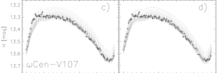
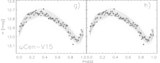
Figure 5: Same as Fig. 4, but for the $H$ band light curve templates.

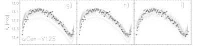
Figure 6: Left (a),d),g),j)) and middle (b),e),h),k)) panels are the same as Fig. 4, but for the $K_{s}$ band light curve templates. The right panels (c),f),i),l) display the fit based on the $K_{s}$ band the J96 light curve template.

We also derived, by applying the template with Equation 1, 100 estimates of $\langle JHK_{s}\rangle_{templ(i)}$, one for each extracted phase point. Subsequently, we estimated the median and the standard deviation of the median over the 100 $\langle JHK_{s}\rangle_{templ(i)}$ extractions. Figures 4, 5 and 6 display the extracted phase points and the fits based on the light-curve templates in the $J$, $H$ and $K_{s}$ bands.

The estimates of $\langle JHK_{s}\rangle_{templ}$—using the Fourier, PEGASUS and J96 templates—of the TVS RRLs are listed in Table 8. The same Table also gives the difference in magnitude ($\Delta\langle JHK_{s}\rangle$) among the different fits.

It is worth noting (see Table 6, columns 2, 3 and 4) that the mean of the residuals with respect to the measured magnitudes is at most 0.010 mag for all the templates. In all cases, the standard deviations are larger than the residuals, meaning that the latter can be considered null within the dispersion. The largest residuals are found in the $H$, band for the RRab1 template: the mean magnitudes estimated from the templates are $\sim$0.01 mag fainter than the measured mean magnitude. This happens because the fit of the $H$-band light curve has minor deviations from the light curve template, and the extracted single phase points follow these deviations. Note that in performing this test we are maximizing the uncertainty, since the error on the individual phase points is estimated as a Gaussian distribution with a $\sigma$ equal to the standard deviation of the analytical fit. Indeed, we found that when using the individual measurements the residuals are systematically smaller.

The comparison between the new and the old $K_{s}$-band templates indicates that the former are on average better than the latter. Indeed, the residuals in the longest period bin (RRab3) of the new templates are one order of magnitude smaller than for the J96 template (–0.001 [Fourier]/0.000 [PEGASUS] mag vs –0.011 mag). Note, however, that the standard deviations are of the same order of magnitude of the difference in offset between our templates and those of J96. Moreover, the standard deviation of the current RRab1 period bin is more than a factor of two smaller than for the J96 template (0.016 [Fourier]/0.016 [PEGASUS] mag vs 0.038 mag). A glance at the data plotted in the right column of Fig. 6, and in particular in the panels d, e) and f), clearly shows the difference.

5.1.2 Light curve templates applied to three phase points

The application of the NIR light-curve templates to individual NIR measurements does require the knowledge of three parameters: i) the period, ii) the luminosity amplitude, and iii) the epoch of the anchor point ($t_{ris}$). The third parameter poses a severe limitation for RRLs because their periods range from a quarter of a day to less than one day. This means that either the pulsation period and the epoch of the anchor point have been estimated with very high accuracy ($\sim$one part per million) or the separation between the time at which the optical and the NIR photometry were collected must be shorter than a few years.

To overcome this limitation we decided to perform a number of tests by assuming that three independent NIR measurements were available. The advantage of this approach is that the light curve template is used as a fitting function. The approach is quite simple and follows the following steps: i) an estimate of the NIR luminosity amplitude using the optical to NIR amplitude ratios available in the literature; ii) a least-squares fit of a light curve including at least three phase points, minimizing the $\chi^{2}$ of two parameters: a shift in phase ($\Delta\phi$) and a shift in magnitude ($\Delta mag$). The functions to be minimized are:

$$F(\phi;\Delta\phi,\Delta mag)=\Delta mag+A_{NIR}\cdot(A_{0}^{F}+\Sigma_{i}A_{i}^{F}\cos{(2\pi i\phi-\phi_{i}-\Delta\phi))}$$ (4)

and

$$P(\phi;\Delta\phi,\Delta mag)=\Delta mag+A_{NIR}\cdot\Big{(}A_{0}^{P}+\Sigma_{i}A_{i}^{P}\exp{\Big{(}-\sin{\Big{(}\dfrac{\pi(\phi-\phi_{i}-\Delta\phi)}{\sigma_{i}^{P}}\Big{)}^{2}}\Big{)}\Big{)}}$$ (5)

for the Fourier and PEGASUS templates, respectively. To further investigate the difference between new and old light-curve templates, the same minimization was also performed using the J96 templates:

$$J(\phi;\Delta\phi,\Delta mag)=\Delta mag+A_{NIR}\cdot(A_{0}^{J}+\Sigma_{i}A_{i}^{J}\cos{(2\pi i\phi-\phi_{i}-\Delta\phi))}$$ (6)

To validate the templates with this approach, we generated 100 triplets of phase points ($\phi_{ij}$,$JHK_{s(ij)}$, where $i$ runs from 1 to 100 and $j$ from 1 to 3). The phases are randomly extracted from a uniform distribution between 0 and 1. The extracted magnitudes, $JHK_{s(ij)}$, were treated following the approach discussed in Section 5.1.1.

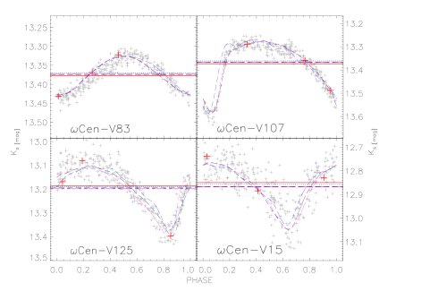
Figure 7: Top-left: Fourier, PEGASUS and J96 template fits applied to RRc variable $\omega$Cen-V83. Gray crosses show the randomly extracted phase points. The red crosses display the three phase points of a single random extraction. The horizontal red line shows the mean magnitude of the variable based on the intensity average fit of the empirical data. The black dashed curve and the horizontal black long-dashed line show the fit with the Fourier template and its mean magnitude. The magenta dashed curve and the horizontal magenta long-dashed line display the same, but for the PEGASUS fit. The blue dotted curve and the horizontal blue dotted line display the same, but for the J96 fit. Top-right: Same as the top-left, but for the RRab variable $\omega$Cen-V107 (RRab1). Bottom-left: Same as the top-left, but for the RRab variable $\omega$Cen-V125 (RRab2). Bottom-right: Same as the top-left, but for the RRab variable $\omega$Cen-V15 (RRab3). Note that, in these panels, the light curves are not phased using $t_{ris}$, but to an arbitrary epoch (HJD=2,350,000) to underline that the three phase points method is independent of the reference epoch.

Once the 100 three-phase point light curves were generated, we performed the fits using Eq.4, 5 and 6. The individual $K_{s}$-band fits are displayed in Fig. 7. We computed 100 estimates of the mean $\langle JHK_{s}\rangle_{templ(i)}$ magnitudes as the integral in intensity over the template fits. The final mean magnitude ($\langle JHK_{s}\rangle_{templ}$) and its uncertainty were determined as the median and the standard deviation of the median over the 100 random estimates of $\langle JHK_{s}\rangle_{templ(i)}$ (see Section 5.1.1). The Table 6 also shows the magnitude differences $\Delta\langle JHK_{s}\rangle$ between the template estimates of the mean magnitudes $\langle JHK_{s}\rangle_{templ(i)}$ and the best estimates of the mean magnitudes based on the fit of the light curve ($\langle JHK_{s}\rangle_{best}$).

Table 5: NIR photometric properties of the $\omega$TVS RRLs.

	$\langle mag\rangle_{best}$	$\langle mag\rangle_{templF1}$	$\langle mag\rangle_{templP1}$	$\langle mag\rangle_{templJ1}$	$\langle mag\rangle_{templF3}$	$\langle mag\rangle_{templP3}$	$\langle mag\rangle_{templJ3}$
	mag	mag	mag	mag	mag	mag	mag
—$\omega$Cen-V83 (RRc)—
$J:$	13.602$\pm$0.004	13.602$\pm$0.014	13.602$\pm$0.014	…	13.602$\pm$0.025	13.603$\pm$0.025	…
$\Delta J:$	…	0.000$\pm$0.014	0.000$\pm$0.014	…	0.000$\pm$0.025	0.001$\pm$0.025	…
$H:$	13.377$\pm$0.006	13.375$\pm$0.037	13.374$\pm$0.037	…	13.378$\pm$0.028	13.378$\pm$0.028	…
$\Delta H:$	…	–0.002$\pm$0.037	–0.003$\pm$0.037	…	0.001$\pm$0.028	0.001$\pm$0.028	…
$K_{s}:$	13.377$\pm$0.005	13.381$\pm$0.038	13.381$\pm$0.038	13.376$\pm$0.038	13.377$\pm$0.026	13.377$\pm$0.026	13.375$\pm$0.025
$\Delta K_{s}:$	…	0.004$\pm$0.038	0.004$\pm$0.038	–0.001$\pm$0.038	0.000$\pm$0.026	0.000$\pm$0.026	–0.002$\pm$0.025
—$\omega$Cen-V107 (RRab1)—
$J:$	13.658$\pm$0.008	13.662$\pm$0.016	13.663$\pm$0.015	…	13.656$\pm$0.083	13.656$\pm$0.083	…
$\Delta J:$	…	0.004$\pm$0.016	0.005$\pm$0.015	…	–0.002$\pm$0.083	–0.002$\pm$0.083	…
$H:$	13.407$\pm$0.006	13.417$\pm$0.025	13.417$\pm$0.026	…	13.397$\pm$0.044	13.396$\pm$0.044	…
$\Delta H:$	…	0.010$\pm$0.025	0.010$\pm$0.026	…	–0.010$\pm$0.044	–0.011$\pm$0.044	…
$K_{s}:$	13.373$\pm$0.006	13.377$\pm$0.016	13.376$\pm$0.016	13.365$\pm$0.038	13.372$\pm$0.026	13.372$\pm$0.027	13.370$\pm$0.046
$\Delta K_{s}:$	…	0.004$\pm$0.016	0.003$\pm$0.016	–0.008$\pm$0.038	–0.001$\pm$0.026	–0.001$\pm$0.027	–0.003$\pm$0.046
—$\omega$Cen-V125 (RRab2)—
$J:$	13.460$\pm$0.005	13.462$\pm$0.019	13.461$\pm$0.021	…	13.451$\pm$0.088	13.453$\pm$0.084	…
$\Delta J:$	…	0.002$\pm$0.019	0.001$\pm$0.021	…	–0.009$\pm$0.088	–0.007$\pm$0.084	…
$H:$	13.206$\pm$0.009	13.207$\pm$0.027	13.208$\pm$0.027	…	13.205$\pm$0.072	13.206$\pm$0.067	…
$\Delta H:$	…	0.001$\pm$0.027	0.002$\pm$0.027	…	–0.001$\pm$0.072	0.000$\pm$0.067	…
$K_{s}:$	13.186$\pm$0.007	13.181$\pm$0.024	13.181$\pm$0.026	13.180$\pm$0.023	13.182$\pm$0.064	13.181$\pm$0.061	13.178$\pm$0.060
$\Delta K_{s}:$	…	–0.005$\pm$0.024	–0.005$\pm$0.026	–0.006$\pm$0.023	–0.004$\pm$0.064	–0.005$\pm$0.061	–0.008$\pm$0.060
—$\omega$Cen-V15 (RRab3)—
$J:$	13.178$\pm$0.006	13.181$\pm$0.020	13.176$\pm$0.021	…	13.169$\pm$0.071	13.168$\pm$0.075	…
$\Delta J:$	…	0.003$\pm$0.020	–0.002$\pm$0.021	…	–0.009$\pm$0.071	–0.010$\pm$0.075	…
$H:$	12.843$\pm$0.008	12.849$\pm$0.026	12.847$\pm$0.027	…	12.835$\pm$0.064	12.837$\pm$0.066	…
$\Delta H:$	…	0.006$\pm$0.026	0.004$\pm$0.027	…	–0.008$\pm$0.064	–0.006$\pm$0.066	…
$K_{s}:$	12.850$\pm$0.007	12.849$\pm$0.026	12.850$\pm$0.027	12.839$\pm$0.029	12.844$\pm$0.066	12.843$\pm$0.069	12.839$\pm$0.058
$\Delta K_{s}:$	…	–0.001$\pm$0.026	0.000$\pm$0.027	–0.011$\pm$0.029	–0.006$\pm$0.066	–0.007$\pm$0.069	–0.011$\pm$0.058

Data Plotted in Fig. 7 show that the residuals are similar to the fits based on a single phase point. Indeed, the residuals are, within the standard deviations, zero. However, the standard deviations of the template fits based on three phase points are larger than those based on a single phase point. The difference is mainly caused by the fact that the three randomly-selected phase points span, in some of the extractions, a very small range ($\Delta\phi\leq 0.05$) in pulsation phase (see Fig. 8. This is also the reason why the residuals are correlated with the difference in phase between the two closest points in phase ($\Delta\phi$).

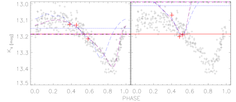
Figure 8: Left: Same as Fig. 7, but for random extraction on the light curve of the RRab variable $\omega$Cen-V125 (RRab2). In this specific case the three randomly extracted phase points are close in phase. The J96 fit does not provide an accurate estimate of the mean magnitude. Right: same as the left, but for an extraction where the three randomly extracted phase points have a smaller difference in phase. In this case the light curve templates do not provide an accurate estimate of the $K_{s}$ band mean magnitude.

The current findings indicate that the light-curve templates used as fitting curves provide accurate mean magnitudes when i) the distance between the phase points is at least 0.1 pulsation cycles. Otherwise, we suggest averaging the two close phase points. ii) the number of available phase points is modest, i.e., larger than two, but smaller than a dozen. Classical analytical fits (Fourier, Spline, PLOESS, PEGASUS…) become more accurate for a larger number of measurements.

5.2 Validation based on OGLE + VVV RR Lyrae

An independent path to validate the current light curve templates is offered by the two different long-term photometric surveys collecting time-series data in the optical (OGLE, (Udalski et al. 1992)) and the NIR (VVV, (Minniti et al. 2010)) of a significant fraction of the Galactic Bulge. The photometric catalogs provided by these surveys can be simultaneously used to validate the $K_{s}$-band templates. Note that we cannot validate the $J$- and $H$-band templates because the VVV survey only collected $K_{s}$-band time series.

The validation relies on the OGLE-IV catalog of 38,257 Bulge RRLs Soszyński et al. (2014). Using a searching radius of 2^′′, we found 2,517 matches in the VVV point source catalog. We used a very small searching radius because this provides a faster selection of the good matches. Obviously, the completeness is modest, but the validation only requires a few variables per period bin. Among them we selected 22 RRLs and the criteria we adopted for the selection are the following: i) – good coverage of the $K_{s}$-band light curve, and in fact they all have at least 38 phase points (80% of them have at least 49 phase points); ii) – good coverage of both the $V$- and the $I$-band light curve to provide accurate estimates of the luminosity amplitudes ($AV$, $AI$) and of the epochs of the mean magnitudes on the rising branch ($t_{ris(V)}$, $t_{ris(I)}$). The phasing of optical and NIR light curves was performed using the pulsation period provided by OGLE. The distribution of these variables among the different period bins is the following: RRc (six), RRab1 (five), RRab2 (five) and RRab3 (six). These variables were called the “Bulge Template Validation Sample” (BTVS) and their pulsation properties are listed in Table 7).

Table 6: Optical properties of the Bulge RRLs adopted to validate the light crve template.

ID (OGLE)	ID (VVV)	$P$	$\langle V\rangle$	$AV$	$t_{risV}$	$\langle I\rangle$	$AI$	$t_{risI}$
		days	mag	mag	HJD	mag	mag	HJD
—RRc—
15624	515514387864	0.30180268	15.576$\pm$0.004	0.433$\pm$0.026	7974.3143	14.844$\pm$0.004	0.249$\pm$0.005	57937.4921
34149	515618496995	0.33202391	16.075$\pm$0.005	0.468$\pm$0.050	7679.3197	15.345$\pm$0.005	0.254$\pm$0.008	57581.7032
35612	515576843509	0.35095553	15.565$\pm$0.005	0.388$\pm$0.026	7681.0746	14.880$\pm$0.004	0.219$\pm$0.006	57610.1786
11254	515548620097	0.38432825	16.514$\pm$0.005	0.447$\pm$0.018	7975.2994	15.249$\pm$0.004	0.253$\pm$0.005	57948.0109
04844	515642803328	0.41666920	16.427$\pm$0.006	0.401$\pm$0.031	7975.1612	15.493$\pm$0.005	0.249$\pm$0.006	57962.2387
34454	515597035098	0.46802773	15.579$\pm$0.004	0.442$\pm$0.022	7675.3195	14.845$\pm$0.004	0.252$\pm$0.005	57653.3189
—RRab1—
13498	515504500749	0.40860801	16.796$\pm$0.007	1.032$\pm$0.043	7974.5872	15.151$\pm$0.005	0.614$\pm$0.010	57948.4284
13432	515504357949	0.45645736	16.381$\pm$0.006	1.138$\pm$0.050	7974.0969	15.319$\pm$0.005	0.641$\pm$0.009	57952.1844
02515	515633495772	0.47702220	16.644$\pm$0.007	0.737$\pm$0.049	7971.7347	14.960$\pm$0.004	0.314$\pm$0.009	57893.0166
09543	515599952081	0.51556077	17.156$\pm$0.008	0.908$\pm$0.042	7974.2127	15.436$\pm$0.005	0.566$\pm$0.010	57974.2092
14578	515597002824	0.54341333	16.319$\pm$0.006	0.924$\pm$0.063	7674.7014	15.289$\pm$0.004	0.582$\pm$0.015	57652.9607
—RRab2—
14806	515567300731	0.56104602	16.127$\pm$0.012	1.203$\pm$0.093	7974.3310	15.281$\pm$0.004	0.771$\pm$0.018	57936.1768
34618	515597253109	0.58514134	15.440$\pm$0.009	1.203$\pm$0.091	7675.1019	14.648$\pm$0.004	0.806$\pm$0.026	57652.8608
11992	515526076762	0.61353035	16.418$\pm$0.007	0.838$\pm$0.032	7974.9419	15.178$\pm$0.004	0.544$\pm$0.005	57954.0771
33059	515657828314	0.63856513	16.244$\pm$0.005	0.843$\pm$0.070	7672.5702	15.215$\pm$0.005	0.531$\pm$0.012	57649.5760
08440	515539115406	0.67505760	16.897$\pm$0.006	0.508$\pm$0.022	7975.4227	15.033$\pm$0.004	0.222$\pm$0.004	57953.1386
—RRab3—
13220	515535451732	0.70481317	16.662$\pm$0.005	0.392$\pm$0.017	7974.4909	15.297$\pm$0.005	0.256$\pm$0.005	57944.1746
10755	515526242552	0.73419273	16.848$\pm$0.006	0.144$\pm$0.008	7975.4450	15.477$\pm$0.005	0.105$\pm$0.005	57954.1314
35604	515551783166	0.77483099	15.670$\pm$0.004	0.665$\pm$0.052	7681.1624	14.760$\pm$0.004	0.419$\pm$0.009	57609.8699
04325	515667731582	0.82203622	16.166$\pm$0.004	0.311$\pm$0.032	7665.9812	14.964$\pm$0.004	0.191$\pm$0.006	57568.9618
14958	515597272287	0.84151947	16.538$\pm$0.006	0.782$\pm$0.070	7674.6534	15.266$\pm$0.004	0.483$\pm$0.011	57652.7685
15775	515545653428	0.87622048	15.655$\pm$0.005	0.523$\pm$0.050	7680.5802	14.711$\pm$0.004	0.330$\pm$0.009	57609.5979

The validation with the BTVS RRLs follows the approach adopted for the $\omega$ Cen RRLs (see Section 5.1). The key idea is to compare the mean magnitude estimated by using the template ($\langle K_{s}\rangle_{templ}$) with the mean magnitude evaluated by using the $K_{s}$ band measurements ($\langle K_{s}\rangle_{best}$). Note that for these objects we will compare eight independent estimates of $\langle K_{s}\rangle_{templ}$, because we will apply Fourier and PEGASUS fits to the light curve parameters based on the $V$- and on the $I$-band data. Moreover, the validation will be applied to both single phase points and triple phase points. We will add suffixes to the subscript of $\langle K_{s}\rangle_{templ[P/F][V/I][1/3]}$. where [$P/F$] indicates that we used either the PEGASUS or the Fourier fit, [$V/I$] indicates that we used either the $V$- or the $I$-band data, and [1/3] indicates that we used either the single phase point or the triple phase points.

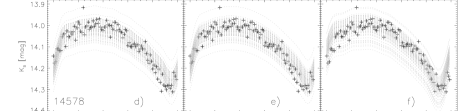
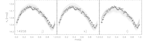
Figure 9: a),b),c) panels: Black pluses represent the randomly extracted $K_{s}$-band phase points over the light curve of the OGLE RRc variable 11254. Gray dashed lines display the template fits to the individual phase points. The Fourier (a), PEGASUS (b) and J96 (c) RRc light curve templates are also displayed. The ID of the RRL is labeled. d),e),f): Same as panels a),b),c), but for the OGLE RRab variable 14578. The RRab1 light curve templates are displayed. g),h),i): Same as panels a),b),c), but for the OGLE RRab variable 14806. The RRab2 light curve templates are displayed. j),k),l): Same as panels a),b),c), but for the OGLE RRab variable 14958. The RRab3 light curve templates are displayed.

The two methods are identical to those described in Section 5.1.1 and 5.1.2. The only difference is that in this case we have more than one RRL per template bin. Therefore, we also estimate the median difference $\langle\Delta\langle K_{s}\rangle\rangle$ for all the RRLs in the period bin. The results are listed in Table 8. Fig. 9 displays the fits to four BTVS RRLs, one for each template bin.

Table 7: NIR photometric properties of the BTVS RRLs.

ID (OGLE)	$\langle K_{s}\rangle_{best}$	$\langle K_{s}\rangle_{templFV1}$	$\langle K_{s}\rangle_{templFI1}$	$\langle K_{s}\rangle_{templPV1}$	$\langle K_{s}\rangle_{templPI1}$	$\langle K_{s}\rangle_{templJ1}$	$\langle K_{s}\rangle_{templFV3}$	$\langle K_{s}\rangle_{templFI3}$	$\langle K_{s}\rangle_{templPV3}$	$\langle K_{s}\rangle_{templPI3}$	$\langle K_{s}\rangle_{templJ3}$
	mag	mag	mag	mag	mag	mag	mag	mag	mag	mag	mag
—RRc—
15624	13.991$\pm$0.021	13.988$\pm$0.039	13.996$\pm$0.034	13.986$\pm$0.038	13.991$\pm$0.035	13.993$\pm$0.036	13.989$\pm$0.027	13.991$\pm$0.029	13.990$\pm$0.025	13.994$\pm$0.029	13.991$\pm$0.029
34149	14.450$\pm$0.018	14.447$\pm$0.018	14.450$\pm$0.016	14.446$\pm$0.017	14.449$\pm$0.015	14.445$\pm$0.022	14.452$\pm$0.014	14.450$\pm$0.011	14.450$\pm$0.013	14.450$\pm$0.011	14.450$\pm$0.011
35612	13.906$\pm$0.012	13.907$\pm$0.026	13.905$\pm$0.023	13.902$\pm$0.024	13.901$\pm$0.021	13.900$\pm$0.027	13.906$\pm$0.019	13.905$\pm$0.015	13.907$\pm$0.015	13.906$\pm$0.018	13.905$\pm$0.015
11254	13.797$\pm$0.027	13.794$\pm$0.028	13.798$\pm$0.025	13.802$\pm$0.029	13.795$\pm$0.025	13.796$\pm$0.030	13.797$\pm$0.021	13.796$\pm$0.019	13.796$\pm$0.020	13.797$\pm$0.019	13.796$\pm$0.019
04844	14.221$\pm$0.024	14.222$\pm$0.069	14.226$\pm$0.066	14.218$\pm$0.077	14.222$\pm$0.073	14.221$\pm$0.070	14.214$\pm$0.044	14.223$\pm$0.038	14.211$\pm$0.039	14.220$\pm$0.042	14.223$\pm$0.038
34454	13.841$\pm$0.011	13.841$\pm$0.022	13.840$\pm$0.020	13.840$\pm$0.023	13.835$\pm$0.024	13.836$\pm$0.025	13.836$\pm$0.016	13.837$\pm$0.014	13.836$\pm$0.017	13.840$\pm$0.016	13.837$\pm$0.014
	$\langle\Delta\langle K_{s}\rangle\rangle$:	–0.001$\pm$0.002	0.000$\pm$0.003	–0.004$\pm$0.004	–0.002$\pm$0.003	–0.003$\pm$0.003	–0.001$\pm$0.003	–0.001$\pm$0.002	–0.001$\pm$0.004	–0.001$\pm$0.002	–0.005$\pm$0.003
—RRab1—
13498	13.803$\pm$0.024	13.814$\pm$0.035	13.811$\pm$0.043	13.803$\pm$0.039	13.801$\pm$0.040	13.806$\pm$0.036	13.802$\pm$0.033	13.792$\pm$0.041	13.794$\pm$0.032	13.798$\pm$0.043	13.792$\pm$0.041
13432	13.488$\pm$0.018	13.488$\pm$0.084	13.486$\pm$0.072	13.489$\pm$0.078	13.492$\pm$0.076	13.491$\pm$0.075	13.501$\pm$0.056	13.501$\pm$0.056	13.527$\pm$0.058	13.485$\pm$0.052	13.501$\pm$0.056
02515	12.622$\pm$0.007	12.639$\pm$0.053	12.631$\pm$0.030	12.638$\pm$0.052	12.631$\pm$0.031	12.636$\pm$0.058	12.644$\pm$0.033	12.636$\pm$0.019	12.645$\pm$0.030	12.635$\pm$0.021	12.636$\pm$0.019
09543	13.297$\pm$0.013	13.299$\pm$0.078	13.307$\pm$0.074	13.302$\pm$0.074	13.286$\pm$0.069	13.298$\pm$0.075	13.279$\pm$0.068	13.301$\pm$0.053	13.284$\pm$0.055	13.283$\pm$0.052	13.301$\pm$0.053
14578	14.086$\pm$0.014	14.084$\pm$0.029	14.087$\pm$0.032	14.090$\pm$0.030	14.078$\pm$0.032	14.079$\pm$0.038	14.077$\pm$0.022	14.084$\pm$0.033	14.076$\pm$0.037	14.082$\pm$0.026	14.084$\pm$0.033
	$\langle\Delta\langle K_{s}\rangle\rangle$:	0.002$\pm$0.010	0.008$\pm$0.006	0.004$\pm$0.007	–0.002$\pm$0.008	0.003$\pm$0.008	0.000$\pm$0.016	0.003$\pm$0.010	–0.009$\pm$0.029	–0.005$\pm$0.010	–0.001$\pm$0.007
—RRab2—
14806	14.226$\pm$0.020	14.229$\pm$0.037	14.228$\pm$0.043	14.230$\pm$0.038	14.231$\pm$0.044	14.227$\pm$0.046	14.223$\pm$0.028	14.223$\pm$0.046	14.228$\pm$0.048	14.220$\pm$0.051	14.223$\pm$0.046
34618	13.635$\pm$0.009	13.637$\pm$0.026	13.636$\pm$0.025	13.636$\pm$0.028	13.640$\pm$0.029	13.629$\pm$0.034	13.634$\pm$0.025	13.635$\pm$0.025	13.633$\pm$0.026	13.638$\pm$0.022	13.635$\pm$0.025
11992	13.677$\pm$0.024	13.682$\pm$0.042	13.670$\pm$0.035	13.673$\pm$0.036	13.675$\pm$0.039	13.670$\pm$0.037	13.666$\pm$0.040	13.668$\pm$0.028	13.672$\pm$0.044	13.662$\pm$0.048	13.668$\pm$0.028
33059	13.945$\pm$0.014	13.940$\pm$0.038	13.945$\pm$0.037	13.937$\pm$0.039	13.948$\pm$0.036	13.935$\pm$0.032	13.940$\pm$0.028	13.940$\pm$0.030	13.946$\pm$0.042	13.936$\pm$0.032	13.940$\pm$0.030
08440	12.802$\pm$0.017	12.806$\pm$0.054	12.806$\pm$0.050	12.800$\pm$0.050	12.796$\pm$0.050	12.796$\pm$0.060	12.803$\pm$0.030	12.798$\pm$0.029	12.800$\pm$0.039	12.795$\pm$0.027	12.798$\pm$0.029
	$\langle\Delta\langle K_{s}\rangle\rangle$:	0.004$\pm$0.004	0.001$\pm$0.004	–0.003$\pm$0.005	0.004$\pm$0.006	–0.006$\pm$0.004	–0.003$\pm$0.005	–0.004$\pm$0.004	–0.002$\pm$0.003	–0.007$\pm$0.007	–0.005$\pm$0.007
—RRab3—
13220	13.762$\pm$0.018	13.764$\pm$0.027	13.755$\pm$0.027	13.765$\pm$0.030	13.761$\pm$0.027	13.746$\pm$0.039	13.756$\pm$0.024	13.755$\pm$0.028	13.754$\pm$0.032	13.759$\pm$0.028	13.755$\pm$0.028
10755	13.748$\pm$0.025	13.746$\pm$0.026	13.746$\pm$0.028	13.749$\pm$0.030	13.740$\pm$0.027	13.748$\pm$0.046	13.749$\pm$0.018	13.746$\pm$0.021	13.750$\pm$0.020	13.745$\pm$0.023	13.746$\pm$0.021
35604	13.680$\pm$0.010	13.679$\pm$0.019	13.683$\pm$0.021	13.679$\pm$0.020	13.679$\pm$0.019	13.674$\pm$0.031	13.678$\pm$0.028	13.682$\pm$0.026	13.679$\pm$0.018	13.677$\pm$0.024	13.682$\pm$0.026
04325	13.569$\pm$0.010	13.576$\pm$0.049	13.566$\pm$0.046	13.566$\pm$0.055	13.573$\pm$0.046	13.563$\pm$0.054	13.570$\pm$0.035	13.569$\pm$0.036	13.565$\pm$0.038	13.569$\pm$0.034	13.569$\pm$0.036
14958	13.750$\pm$0.011	13.749$\pm$0.017	13.748$\pm$0.016	13.746$\pm$0.017	13.749$\pm$0.017	13.743$\pm$0.020	13.751$\pm$0.021	13.747$\pm$0.015	13.753$\pm$0.013	13.754$\pm$0.016	13.747$\pm$0.015
15775	13.579$\pm$0.012	13.577$\pm$0.030	13.580$\pm$0.023	13.570$\pm$0.026	13.578$\pm$0.027	13.565$\pm$0.036	13.579$\pm$0.018	13.577$\pm$0.021	13.576$\pm$0.025	13.574$\pm$0.022	13.577$\pm$0.021
	$\langle\Delta\langle K_{s}\rangle\rangle$:	–0.001$\pm$0.004	–0.002$\pm$0.004	–0.002$\pm$0.004	–0.001$\pm$0.004	–0.007$\pm$0.006	0.000$\pm$0.003	–0.002$\pm$0.003	–0.002$\pm$0.004	–0.003$\pm$0.003	–0.009$\pm$0.006

In this context it is worth mentioning that two (OGLE ID: 34618, 11992) out of the 22 BTVS RRLs, both belonging to the RRab2 period bin, are Blazhko RRLs. The amplitude modulation is 0.2 mag in the $I$ band and 0.3 mag in the $V$ band. The Blazhko modulation does not significantly affect the mean magnitude ($\Delta\langle K_{s}\rangle$) for two main reasons. i) The OGLE data are well sampled and we could estimate the average amplitude over the Blazhko cycle. ii) Blazhko variables with extreme amplitude modulation, i.e., 0.5 mag in $V$, and sampled only across the phases of the maximum will be affected by an error of the order of 0.4 mag in $V$ amplitude. The impact of this amplitude uncertainty on the mean magnitude estimated by using the template is minimal, indeed it is of the order of 0.002 mag in the $J$ band and even smaller for the other bands. Note, however, that this limitation becomes severe for the J96 RRab templates, because the different light-curve templates are based on the luminosity amplitude. The use of a wrong template causes a systematic error in the mean magnitude of the order of a few hundredths of a magnitude.

6 Application of the new light curve templates to Reticulum RRLs

Reticulum is an extragalactic Globular Cluster associated with the halo of the Large Magellanic Cloud (LMC). It hosts a sizable sample of RRLs (32 in total Walker 1992) and it is an interesting workbench, because the J96 light curve templates were adopted by Dall’Ora et al. (2004) to derive the mean $K_{s}$-band magnitudes of 30 RRLs that were observed with SOFI at NTT. However, the mean $J$-band magnitudes were estimated as the mean of the measurements. The number of measurements was limited, typically 46 unbinned phase points, which means on average ten binned phase points (see below). This means that the classical analytical fits (spline, Fourier series) could be applied. Moreover, the $J$-band light curve templates were not available. These are the reasons why the authors focused their cluster distance determinations only on the $K_{s}$ band PL relation. The new light-curve templates will be used to provide new $J$- and $K_{s}$-band mean magnitudes, new NIR PL relations, and—in turn—new cluster distance determinations.

6.1 Phasing of the data and application of the light curve templates

We plan to use the photometric data collected by Dall’Ora et al. (2004), but we will derive new NIR ($JK_{s}$) curves. In particular, we plan to take advantage of the new pulsation periods and epoch of the anchor point recently provided by (Kuehn et al. 2013). Moreover, the SOFI $JK_{s}$-band data were binned using the same approach adopted in Braga et al. (2018). The data collected in one dither pattern were binned into a single phase point using a time interval of 108 sec. The binned $J$- and $K_{s}$-band light curves have a number of phase points ranging from ten to fourteen. The $J$- and $K_{s}$-band light curves of three variables, V10 (RRc), V19 (RRab1) and V5 (RRab2), are displayed in Fig. 10 together with the template fits (black dashed lines) and the mean magnitude (green solid line).

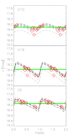
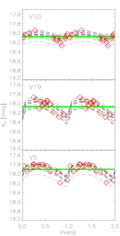
Figure 10: Top: $J$ (left panel) and $K_{s}$ (right panel) band light curve for the RRc variable V10. The red diamonds display the binned phase points. The black dashed curves show the light curve template applied to the individual binned phase points. The thick green line displays the mean magnitude listed in Table 9. Middle: Same as the top, but for the RRab variable V19. Bottom: Same as the top, but for the RRab variable V5.

We have folded the light curves with the periods published by Kuehn et al. (2013). However, the decimal places provided in their Table 1 and 2 are limited and for seven RRLs (V3, V4, V11, V15, V24, V28, V32, using the new notation introduced by Kuehn et al. 2013), the folded light curves show significant phase drifts. Therefore, for these RRLs we estimated our own periods, based on their $V$-band light curves (see Table 9).

Table 8: Optical and NIR photometric properties of Reticulum RRLs.

ID	Period	$\langle V\rangle$	$AV$	$t_{ris}$	$\langle J\rangle$	$\langle K\rangle$
	days	mag	mag	days	mag	mag
V01	0.50993000	19.030$\pm$0.018	1.15$\pm$0.05	55595.5036	…	…
V02	0.61869000	19.084$\pm$0.018	0.63$\pm$0.03	55595.6344	18.09$\pm$0.11	17.84$\pm$0.06
V03	0.35354552	19.053$\pm$0.018	0.42$\pm$0.02	55595.7200	18.24$\pm$0.04	18.03$\pm$0.08
V04	0.35322097	19.059$\pm$0.102	0.41$\pm$0.02	55595.6335	18.29$\pm$0.07	18.08$\pm$0.06
V05	0.57185000	19.042$\pm$0.018	0.90$\pm$0.04	55595.6783	18.15$\pm$0.05	17.90$\pm$0.07
V06	0.59526000	19.105$\pm$0.019	0.59$\pm$0.03	55595.9238	18.17$\pm$0.10	17.86$\pm$0.10
V07	0.51044000	19.011$\pm$0.019	1.14$\pm$0.04	55595.3900	18.21$\pm$0.06	18.00$\pm$0.11
V08	0.64496000	19.075$\pm$0.018	0.41$\pm$0.02	55595.6523	18.06$\pm$0.09	17.69$\pm$0.14
V09	0.54496000	19.007$\pm$0.018	0.80$\pm$0.04	55595.5549	18.22$\pm$0.05	17.94$\pm$0.07
V10	0.35256000	19.079$\pm$0.018	0.43$\pm$0.02	55595.2460	18.31$\pm$0.08	18.07$\pm$0.06
V11	0.35539753	19.072$\pm$0.020	0.44$\pm$0.03	55595.3895	18.34$\pm$0.07	18.11$\pm$0.07
V12	0.29627000	18.983$\pm$0.016	0.22$\pm$0.02	55595.5187	18.40$\pm$0.06	18.24$\pm$0.08
V13	0.60958000	19.093$\pm$0.019	0.72$\pm$0.04	55595.2470	18.13$\pm$0.08	17.81$\pm$0.07
V14	0.58661000	19.059$\pm$0.019	0.69$\pm$0.02	55595.6339	18.21$\pm$0.14	17.95$\pm$0.10
V15	0.35427716	19.092$\pm$0.019	0.42$\pm$0.03	55595.5856	18.31$\pm$0.07	18.11$\pm$0.10
V16	0.52290000	19.054$\pm$0.018	1.12$\pm$0.05	55595.7704	18.27$\pm$0.06	17.98$\pm$0.08
V17	0.51241000	19.041$\pm$0.019	1.14$\pm$0.10	55595.4844	18.25$\pm$0.22	18.09$\pm$0.11
V18	0.56005000	19.080$\pm$0.019	0.93$\pm$0.04	55595.4833	18.14$\pm$0.07	17.91$\pm$0.06
V19	0.48485000	19.056$\pm$0.019	1.22$\pm$0.04	55595.6953	18.38$\pm$0.09	18.07$\pm$0.08
V20	0.56075000	19.123$\pm$0.021	0.71$\pm$0.03	55595.6680	18.26$\pm$0.16	17.89$\pm$0.09
V21	0.60700000	19.094$\pm$0.019	0.70$\pm$0.03	55596.1339	18.19$\pm$0.17	17.76$\pm$0.12
V22	0.51359000	19.069$\pm$0.018	0.89$\pm$0.04	55595.6068	18.22$\pm$0.08	17.91$\pm$0.12
V23	0.46863000	19.162$\pm$0.021	0.95$\pm$0.04	55595.8827	18.33$\pm$0.18	18.10$\pm$0.09
V24	0.34752424	19.092$\pm$0.020	0.40$\pm$0.02	55595.8014	18.38$\pm$0.06	18.09$\pm$0.06
V25	0.32991000	19.048$\pm$0.018	0.50$\pm$0.02	55595.4580	18.39$\pm$0.06	18.21$\pm$0.14
V26	0.65696000	19.087$\pm$0.018	0.28$\pm$0.02	55595.3645	18.11$\pm$0.11	17.75$\pm$0.09
V27	0.51382000	19.062$\pm$0.020	1.22$\pm$0.07	55595.5439	18.16$\pm$0.16	17.95$\pm$0.09
V28	0.31994112	18.999$\pm$0.018	0.49$\pm$0.02	55595.3373	18.37$\pm$0.08	18.14$\pm$0.10
V29	0.50815000	19.063$\pm$0.018	1.14$\pm$0.04	55595.4709	18.36$\pm$0.11	18.06$\pm$0.07
V30	0.53501000	19.012$\pm$0.019	1.04$\pm$0.05	55595.7935	18.28$\pm$0.12	17.99$\pm$0.07
V31	0.50516000	19.087$\pm$0.018	1.07$\pm$0.05	55595.5749	18.31$\pm$0.08	18.03$\pm$0.07
V32	0.35225470	19.049$\pm$0.017	0.42$\pm$0.02	55595.7202	…	…

Subsequently, we estimated $t_{ris}$ from the $V$-band light curves provided by Kuehn et al. (2013). We fit the optical light curves using the PLOESS method described in Braga et al. (2018). We found that the difference between our $V$-band mean magnitudes and those provided by Kuehn et al. (2013) is negligible, with a mean of 0.003 mag, a standard deviation of 0.012 mag and a maximum difference of 0.035 mag. On the basis of the new periods and of the new epochs ($t_{ris}$), we folded the NIR light curves.

It is worth mentioning that Reticulum hosts six mixed-mode RRLs (RRd) and we have NIR data for five of them (except V32). We do not provide templates for this type of variable, but since the dominant mode is the first overtone, we decided to apply the RRc light curve template to these variables.

To apply the template, we need an estimate of the optical amplitudes of the RRLs and of the NIR-to-optical amplitude ratios (Braga et al. 2018) to rescale the template function. We decided to adopt our own $V$-band amplitudes—estimated from the PLOESS fits derived in Section 6.1—because they differ from those published by Kuehn et al. (2013). The mean difference $\Delta AV=AV_{our}-AV_{K13}$ is –0.08 mag, with a standard deviation of 0.07 mag and a maximum difference of –0.32 mag. We obtained smaller luminosity amplitudes because, for Blazhko and RRd variables, we did not fit the brighter/fainter envelopes of the data (Kuehn et al. (2013)) since we are interested in the application of the template to determine their NIR mean magnitudes.

We then applied to each phase point of the NIR binned light curve both the PEGASUS and the Fourier light curve templates. This means that we estimated two mean magnitudes ($\langle J\rangle_{i}$, $\langle K_{s}\rangle_{i}$) per phase point, where $i$ indicates the $i$-th phase point. Interestingly enough, the Fourier and the PEGASUS templates provide, within the photometric uncertainty of the individual phase points, similar estimates of both $\langle J\rangle_{i}$ and $\langle K_{s}\rangle_{i}$. The final values of $\langle J\rangle$ and $\langle K_{s}\rangle$ are the medians of all the $\langle J\rangle_{i}$ and $\langle K_{s}\rangle_{i}$. They are listed in Table 9, together with their standard deviations.

6.2 New empirical $J$ and $K_{s}$ PL relations and the distance to Reticulum

We derived the PL relations in the $J$ and $K_{s}$ band after correcting the NIR mean magnitudes for reddening. Following the same arguments of Muraveva et al. (2018b), we adopted the cluster reddening (E(B–V)=0.03$\pm$0.02 mag) originally derived by (Walker 1992). We also adopted $R_{V}$=3.1 and the optical-to-NIR extinction ratios by Cardelli et al. (1989). Note that in the current PL relations the periods of RRc and RRd variables were “fundamentalized”, i.e., we adopted $\log P_{F}=\log P_{FO}$+0.128 (Kuehn et al. 2013). We obtained the following PL relations, where $J_{0}$ and $K_{s0}$ indicate the un-reddened magnitudes:

$$J_{0}=(17.78\pm 0.05)-(1.58\pm 0.17)\cdot\log{P}$$ (7)

$$K_{s0}=(17.29\pm 0.04)-(2.40\pm 0.15)\cdot\log{P}$$ (8)

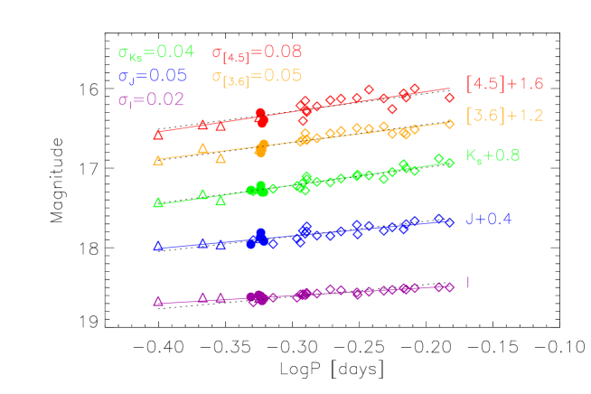
Figure 11: $I$-, $J$-, $K_{s}$- [3.6]- and [4.5]-band PL relations of Reticulum RRLs. Diamonds display RRab variables, triangles RRc variables and circles the RRd variables. Purple, blue, green, orange and red symbols display the un-reddened mean magnitudes in the $I$, $J$, $K_{s}$ [3.6] and [4.5] bands, respectively. The solid lines display the empirical PL relations (Equations 7, 8, 9, 10 and 11). The dashed black lines display the theoretical PLZ relations by Marconi et al. (2015); Neeley et al. (2017), at [Fe/H]=–1.70 (Suntzeff et al. 1992, transformed into the Carretta et al. 2009 metallicity scale) and artificially shifted in magnitude. The $I$ was only shifted for the current value of the true distance modulus. The standard deviation of the relations are labelled on the top-left corner.

The coefficients of the current empirical PL$K_{s}$ relation and their standard deviations are, within the errors, very similar to those obtained by Dall’Ora et al. (2004). The standard deviation of the PL$J$ relation is larger than in the PL$K_{s}$ relation (0.05 vs 0.04 mag), as suggested by theoretical predictions (0.06 mag Marconi et al. 2015). Finally, we have estimated the true distance modulus ($\mu$) of Reticulum using the new NIR mean magnitudes ($J$,$K_{s}$) and the theoretical Global PLZ relations provided by Marconi et al. (2015, , Marconi et al (2018, in prep.)). We have adopted the spectroscopic iron abundance obtained by Suntzeff et al. (1992) from Reticulum red giants, transformed into the (Carretta et al. 2009) metallicity scale ([Fe/H]=–1.70). We found $\mu_{J}$=18.47$\pm$0.10$\pm$0.03 mag and $\mu_{Ks}$=18.49$\pm$0.09$\pm$0.05 mag, where the first is the standard error of the mean and the second the standard deviation. The latter was computed as the squared sum of the average uncertainty on the mean magnitudes only, since the uncertainty in the extinction and the propagation of the uncertainties in the calibrating PLZ coefficients vanish when square-summed.

The true distance modulus obtained by Dall’Ora et al. (2004) from the same data, but using a different theoretical $K_{s}$-band PLZ (Bono et al. 2003) relation, was $\mu$=18.52$\pm$0.05 mag. The three distance determinations agree quite well, and indeed the difference is within 1$\sigma$.

The distance to Reticulum was estimated by Kuehn et al. (2013) using the visual mean magnitude-metallicity relation relation provided by Catelan & Cortés (2008), a cluster metallicity of [Fe/H]=–1.66 (Mackey & Gilmore 2004, in the Zinn & West 1984 scale) and a cluster reddening of E(B–V)=0.016 mag (Schlegel et al. 1998). They found a true distance modulus of 18.40$\pm$0.20 mag. They also adopted the $I$-band PL relation provided by Catelan et al. (2004), the same cluster reddening and the Cardelli et al. (1989) reddening law and they found a true distance modulus of 18.47$\pm$0.06 mag.

The Reticulum true distance modulus was more recently estimated by Muraveva et al. (2018b) using Mid-Infrared (MIR) mean magnitudes, collected with IRAC at Spitzer, for 24 ([3.6]) and 23 ([4.5]) RRLs. They found true distance moduli of $\mu$=18.32$\pm$0.06 mag ([3.6]) and 18.34$\pm$0.08 mag ([4.5]) mag, adopting two empirical zero-points based on Gaia DR1 (Gaia Collaboration et al. 2016b) and Gaia DR2 (Gaia Collaboration et al. 2018; Clementini et al. 2018) trigonometric parallaxes. They also adopted a third independent zero-point based on HST (Benedict et al. 2011) trigonometric parallaxes for five field RRLs, and found that this calibration provides distances that are 0.10 mag larger than those based on the Gaia calibrations. Note that Muraveva et al. (2018b) adopted a different metal content ([Fe/H]=–1.66, Mackey & Gilmore 2004, in the Zinn & West 1984 scale), but the difference in cluster metallicity affects the distance only at the level of 0.01 mag.

The cluster distance found by Muraveva et al. (2018b) is smaller than the geometric distance to the LMC found by Pietrzyński et al. (2013) ($\mu_{LMC}$=18.493$\pm$0.008$\pm$0.047 mag) from late-type eclipsing binaries and by (Inno et al. 2016) ($\mu_{LMC}=18.48\pm 0.10$ mag) from Classical Cepheids with optical/NIR ($VIJHK_{s}$; $\sim$4,000) and MIR ($w_{1}$, WISE photometric system; $\sim$2,600) measurements. Classical Cepheids are young (t$<$300 Myr), intermediate-mass stars and mainly trace the disk/bar of the galaxy. On the basis of their relative distances (Inno et al. 2016) found an LMC depth of the order of $\sim\pm$0.2 mag. This suggests that the intrinsic spread in distance along the line of sight is roughly the 10% of its distance ($\sim\pm$5 kpc).

To discuss in more detail the position of Reticulum compared with LMC barycenter we provide independent and homogeneous distance moduli based on both optical and MIR measurements available in the literature. This approach is further strengthened by the recent findings by Muraveva et al. (2018a) suggesting, based on a large sample of Gaia DR2 trigonometric parallaxes (Arenou et al. 2018), that the coefficients of the metallicity term predicted by pulsation models agree quite well with observations. We adopted the MIR mean magnitudes provided by Muraveva et al. (2018b) and the MIR theoretical PLZ relations provided by Marconi et al. (2015, see Fig. 11); Neeley et al. (2017, see Fig. 11). We found the following empirical PL relations

$$[3.6]_{0}=(17.24\pm 0.06)-(2.12\pm 0.21)\cdot\log{P}$$ (9)

$$[4.5]_{0}=(17.13\pm 0.08)-(2.52\pm 0.29)\cdot\log{P}$$ (10)

and true distance moduli of $\mu_{[3.6]}=$18.30$\pm$0.06$\pm$0.05 and of $\mu_{[4.5]}=$18.31$\pm$0.08$\pm$0.08 mag. The new true distance moduli are in remarkable agreement with distances provided by Muraveva et al. (2018b). The distances based on MIR mean magnitudes are systematically smaller then those based on NIR mean magnitudes, but the difference is of the order of 1$\sigma$. To further investigate the possible systematics affecting the current distance determinations we also estimated the true distance modulus from the $I$-band mean magnitudes provided by Kuehn et al. (2013). We found the following empirical PL relation

$$I_{0}=(18.30\pm 0.03)-(1.00\pm 0.10)\cdot\log{P}$$ (11)

and a true distance modulus of $\mu_{I}=$18.51$\pm$0.07$\pm$0.05 mag (see the purple line in Fig. 11). Finally, we also adopted the optical Period-Wesenheit (PW) relations for a threefold reason. i) These distance diagnostics are independent, by construction, of the reddening uncertainties. ii) Using some specific combinations of filters, they are minimally affected by metal content (Marconi et al. 2015). iii) They mimic a period-luminosity-color relation (Madore 1982; Marconi et al. 2015; Neeley et al. 2017). However, they rely on the assumption that the adopted reddening law is universal. We adopted the PW($V$,$B-I$) relation by Marconi et al. (2015) and the optical $VBI$ mean magnitudes provided by Kuehn et al. (2013) and we found $\mu=$18.52$\pm$0.03$\pm$0.03 mag. The mean of the homogeneous NIR (PLZ: $J$,$K_{s}$), MIR (PLZ: [3.6], [4.5]) and optical (PLZ: $I$; PW($V$,$B-I$)) distance determinations gives a mean cluster distance of $\mu=$18.47$\pm$0.02$\pm$0.06 mag.

The current estimates support the evidence that Reticulum belongs to the LMC halo. In particular, the use of optical, NIR and MIR data suggests that it is located $\sim$1 kpc closer than the LMC barycenter, although it must be kept in mind that the systematics are of the same order of magnitude of this shift. Distance determinations based on MIR data and on Gaia trigonometric parallaxes suggest that Reticulum might be even closer ($\sim$3 kpc, Muraveva et al. (2018b)). More accurate estimates require a novel approach as recently suggested by Bono et al. (2018) to simultaneously estimate the cluster mean metallicity, reddening and distance.

7 Summary and final remarks

In this work, we have provided the NIR ($JHK_{s}$) light curve templates of RRab and RRc variables. In the following, we summarize the most interesting results and discuss in more detail some relevant issues.

Homogeneous photometry — We publish $JHK_{s}$ time series, in the 2MASS photometric system, of 254 RRLs in the GGCs $\omega$ Cen, M4 and in the field of the Milky Way. The latter sample was obtained from heterogeneous literature data in four different photometric systems (CIT, SAAO, UKIRT and ESO) which were homogenized. The overall sample includes both photoelectric and CCD data, collected at telescopes in a wide range of diameter classes (1.3m to 8m). We provide NIR ($JHK_{s}$) characterization (mean magnitudes, light amplitudes, epochs of the mean magnitude on the rising branch) for 94 RRab and 51 RRc variables that were used to generate the light-curve templates.

Light-curve templates — We provide a total of 24 light-curve templates of RRLs: these are divided into Fourier and multi-Gaussian series (PEGASUS) fits of four period bins (one for the RRc and three for the RRab variables) and three photometric bands ($J$, $H$ and $K_{s}$). The Fourier and PEGASUS series range from the fourth to the seventh order and from the second to the sixth order, respectively. The Fourier templates show residuals with respect to the normalized cumulated light curves used to generate them that are smaller than those corresponding to the PEGASUS templates. However, the latter show fewer secondary, unphysical features (bumps and dips) and their residuals are still smaller than 0.005 normalized mag. We provide also the phases of minimum and maximum light for all the light-curve templates, in order to make it easier for future users to adopt the template even when lacking the epoch of the mean magnitude on the rising branch, which is less commonly reported than the epoch of maximum in large surveys.

Template validation — We have validated our templates and compared our $K_{s}$-band templates to those by J96. The tests were performed on both a subsample of four RRLs in $\omega$ Cen (one per template bin), that were not used to generate the templates, and on a set of 22 Galactic bulge RRLs for which we have $VI$ time series from OGLE and $K_{s}$-band time series from the VVV survey. We have checked that, within the dispersion, the mean magnitudes derived by applying the template and the best estimate of the mean magnitude (i.e., the integral over the fit of the light curve, converted into intensities) are the same. The largest offset is of 0.01 mag (with a standard deviation of 0.04 mag), for the $H$-band template of short-period RRab variables (RRab1 template bin), which are also the ones with the largest amplitudes, meaning that they are more prone to uncertainties. Compared to our $K_{s}$ templates, the J96 templates provide results which are similar, showing offsets either comparable or—sometimes—larger than ours.

Reticulum — We have collected literature $JK_{s}$ time series for 30 over 32 RRLs in the LMC globular cluster Reticulum (Dall’Ora et al. 2004). Using $BV$ time series for the same RRLs (Kuehn et al. 2013), we derived the periods and $t_{ris}$ to apply our templates and estimated NIR mean magnitudes. We derived new empirical PL$JK_{s}$ relations, and in turn, new accurate and precise estimates of the distance to Reticulum. We found true distance moduli that agree quite well with each other ($\mu_{J}=$18.47$\pm$0.10$\pm$0.03 mag, $\mu_{Ks}=$18.49$\pm$0.09$\pm$0.05 mag) and with literature values. We adopted homogeneous calibrations for MIR ([3.6], [4.5]) and optical ($I$) PLZ relations and for the optical PW($V$,$B-I$) relation together with mean magnitudes provided by Muraveva et al. (2018b) and by Kuehn et al. (2013). We found a mean cluster true distance modulus of $\mu=$18.47$\pm$0.02$\pm$0.06 mag. According to the most accurate and recent LMC distance determinations (Pietrzyński et al. 2013; Inno et al. 2016), the current $\mu$ estimate for Reticulum indicates that this cluster is $\sim$1 kpc closer to us than the LMC itself.

In the following we briefly outline some of the most relevant developments of the current project supporting the non-trivial effort for new NIR light-curve templates for RRLs.

Distance Scale — Future ground-based Extremely Large Telescopes (ELT, TMT, GMT) and space observing facilities (JWST, EUCLID, WFIRST) have been designed to reach their peak performance in the NIR regime. This means that a few NIR measurements of variables already identified and characterized in the NIR will allow us to fully exploit the RR Lyrae distance scale in Local Group and in Local Volume galaxies. Note that this opportunity fits within a context in which Gaia will provide exquisite calibration for both the zero point and the slope of the diagnostics we are currently using to estimate individual RR Lyrae distances (Gaia Collaboration et al. 2016b, a; Arenou et al. 2018). Moreover, LSST will provide an unprecedented wealth of optical time series, and in turn a complete census of evolved variables in the nearby Universe (Oluseyi et al. 2012). These are crucial prior conditions to reach a precision of the order of 1% on individual RRL distances and an accuracy better than 3% on the Hubble constant (Carnegie RR Lyrae Program Beaton et al. 2016).

Light curve characterization — Light-curve templates also provide the opportunity to improve the accuracy of the fit of the light curve when either a single or a few measurements are available. Note that this opportunity becomes even more relevant for NIR photometric surveys, like VVV+VVV-X (Minniti et al. 2010), that collect time-series data in the $K_{s}$-band and just a few measurements in the $J$ and $H$ bands. Accurate NIR mean magnitudes are, together with optical mean magnitudes, a fundamental ingredient for constraining the distance, the reddening and the metal content of field and cluster RR Lyrae using the recent algorithm (REDIME) suggested by Bono et al. (2018).

Envelope tomography — Our knowledge of linear and nonlinear phenomena taking place along the pulsation cycle of a variable star is still limited to a handful of objects. There is solid evidence that moving from the optical to the NIR regime luminosity changes are mainly dominated by variations of radius instead of temperature (Bono et al. 2001; Madore et al. 2013). However, we still lack accurate investigations of shock formation and propagation based on NIR spectroscopic diagnostics. The NIR light-curve templates provide the opportunity to trace the color ($V-K$) variation along the pulsation cycle, and in turn, the temperature variation. This information is crucial for estimating atmospheric parameters of spectra including a limited number of ionized/neutral heavy element lines (Sollima et al. 2006, ,Magurno et al. 2018, in preparation).

It goes without saying that it is a real pleasure to develop a new tool to be used by the astronomical community, but it is even more appealing to use it on a broad range of stellar systems.

Appendix A Estimate of the phase of the anchor point ($t_{ris}$)

To derive $t_{ris}$, we adopted the following approach. We selected, for each star, one filter for which either the optical ($B$, $V$) or the NIR ($J$) light curve is regular and well sampled. Then, we fit the light curve with either a PLOESS (all the MW RRLs and part of the $\omega$ Cen RRLs) or a spline fit (all the M4 RRLs and the remaining part of the $\omega$ Cen RRLs) and derived the mean magnitude from the intensity integral of the analytic fit.

We then interpolated the phase at which the rising branch of the fit intersects the mean magnitude (${\phi}_{0}$). Finally, $t_{ris}$ could be obtained as $t_{i}-(({\phi}_{i}-{\phi}_{0})\cdot P)-P$, where $t_{i}$ and ${\phi}_{i}$ are the epoch and the phase of the $i$-th phase point of the light curve, respectively. This specific phase point was called the “anchor point”. In principle, any of the phase points in the light curve could be an anchor point. However, we have used an interactive procedure 1) to avoid selecting an anchor point which deviates from the others due to either period changes or phase shifts with time; and 2) to sort the phase points from the most recent to the oldest, to obtain a final estimate of $t_{ris}$ that is as recent as possible. The latter might seem a non-necessary requirement, but it is crucial to have reference epochs which are as close as possible in time to the NIR measurements over which the templates will be applied.

References

- Arenou et al. (2018) Arenou, F., Luri, X., Babusiaux, C., et al. 2018, A&A, 616, A17
- Barnes et al. (1992) Barnes, III, T. G., Moffett, T. J., & Frueh, M. L. 1992, PASP, 104, 514
- Barnes et al. (1988) Barnes, III, T. G., Moffett, T. J., Hawley, S. L., Slovak, M. H., & Frueh, M. L. 1988, ApJS, 67, 403
- Beaton et al. (2016) Beaton, R. L., Freedman, W. L., Madore, B. F., et al. 2016, ApJ, 832, 210
- Benedict et al. (2011) Benedict, G. F., McArthur, B. E., Feast, M. W., et al. 2011, AJ, 142, 187
- Bono et al. (1997) Bono, G., Caputo, F., Cassisi, S., Incerpi, R., & Marconi, M. 1997, ApJ, 483, 811
- Bono et al. (2001) Bono, G., Caputo, F., Castellani, V., Marconi, M., & Storm, J. 2001, MNRAS, 326, 1183
- Bono et al. (2003) Bono, G., Caputo, F., Castellani, V., et al. 2003, MNRAS, 344, 1097
- Bono et al. (2000) Bono, G., Castellani, V., & Marconi, M. 2000, ApJ, 532, L129
- Bono et al. (2018) Bono, G., Iannicola, G., Braga, V. F., et al. 2018, ArXiv e-prints [arXiv:1811.07069]
- Bono & Stellingwerf (1994) Bono, G. & Stellingwerf, R. F. 1994, ApJS, 93, 233
- Braga et al. (2016) Braga, V. F., Stetson, P. B., Bono, G., et al. 2016, AJ, 152, 170
- Braga et al. (2018) Braga, V. F., Stetson, P. B., Bono, G., et al. 2018, AJ, 155, 137
- Cacciari et al. (1992) Cacciari, C., Clementini, G., & Fernley, J. A. 1992, ApJ, 396, 219
- Cacciari et al. (1987) Cacciari, C., Clementini, G., Prevot, L., et al. 1987, A&AS, 69, 135
- Cacciari et al. (2005) Cacciari, C., Corwin, T. M., & Carney, B. W. 2005, AJ, 129, 267
- Caputo et al. (2000) Caputo, F., Castellani, V., Marconi, M., & Ripepi, V. 2000, MNRAS, 316, 819
- Cardelli et al. (1989) Cardelli, J. A., Clayton, G. C., & Mathis, J. S. 1989, ApJ, 345, 245
- Carney & Latham (1984) Carney, B. W. & Latham, D. W. 1984, ApJ, 278, 241
- Carpenter (2001) Carpenter, J. M. 2001, AJ, 121, 2851
- Carretta et al. (2009) Carretta, E., Bragaglia, A., Gratton, R., D’Orazi, V., & Lucatello, S. 2009, A&A, 508, 695
- Catelan & Cortés (2008) Catelan, M. & Cortés, C. 2008, ApJ, 676, L135
- Catelan et al. (2004) Catelan, M., Pritzl, B. J., & Smith, H. A. 2004, ApJS, 154, 633
- Clementini et al. (1990) Clementini, G., Cacciari, C., & Lindgren, H. 1990, A&AS, 85, 865
- Clementini et al. (2018) Clementini, G., Ripepi, V., Molinaro, R., et al. 2018, ArXiv e-prints [arXiv:1805.02079]
- Dall’Ora et al. (2004) Dall’Ora, M., Storm, J., Bono, G., et al. 2004, ApJ, 610, 269
- Drake et al. (2009) Drake, A. J., Djorgovski, S. G., Mahabal, A., et al. 2009, ApJ, 696, 870
- Fernley et al. (1990) Fernley, J. A., Skillen, I., Jameson, R. F., et al. 1990, MNRAS, 247, 287
- Freedman & Madore (2010) Freedman, W. L. & Madore, B. F. 2010, ApJ, 719, 335
- Gaia Collaboration et al. (2016a) Gaia Collaboration, Brown, A. G. A., Vallenari, A., et al. 2016a, A&A, 595, A2
- Gaia Collaboration et al. (2018) Gaia Collaboration, Brown, A. G. A., Vallenari, A., et al. 2018, A&A
- Gaia Collaboration et al. (2016b) Gaia Collaboration, Prusti, T., de Bruijne, J. H. J., et al. 2016b, A&A, 595, A1
- Gonzalez et al. (2012) Gonzalez, O. A., Rejkuba, M., Zoccali, M., et al. 2012, A&A, 543, A13
- Hajdu et al. (2018) Hajdu, G., Dékány, I., Catelan, M., Grebel, E. K., & Jurcsik, J. 2018, ApJ, 857, 55
- Inno et al. (2016) Inno, L., Bono, G., Matsunaga, N., et al. 2016, ApJ, 832, 176
- Inno et al. (2015) Inno, L., Matsunaga, N., Romaniello, M., et al. 2015, A&A, 576, A30
- Jones et al. (1996) Jones, R. V., Carney, B. W., & Fulbright, J. P. 1996, PASP, 108, 877
- Jones et al. (1988a) Jones, R. V., Carney, B. W., & Latham, D. W. 1988a, ApJ, 326, 312
- Jones et al. (1988b) Jones, R. V., Carney, B. W., & Latham, D. W. 1988b, ApJ, 332, 206
- Jones et al. (1987) Jones, R. V., Carney, B. W., Latham, D. W., & Kurucz, R. L. 1987, ApJ, 312, 254
- Jones et al. (1992) Jones, R. V., Carney, B. W., Storm, J., & Latham, D. W. 1992, ApJ, 386, 646
- Kaluzny et al. (1997) Kaluzny, J., Kubiak, M., Szymanski, M., et al. 1997, A&AS, 125, 343
- Kaluzny et al. (2004) Kaluzny, J., Olech, A., Thompson, I. B., et al. 2004, A&A, 424, 1101
- Kochanek et al. (2017) Kochanek, C. S., Shappee, B. J., Stanek, K. Z., et al. 2017, PASP, 129, 104502
- Koen et al. (2007) Koen, C., Marang, F., Kilkenny, D., & Jacobs, C. 2007, MNRAS, 380, 1433
- Kuehn et al. (2013) Kuehn, C. A., Dame, K., Smith, H. A., et al. 2013, AJ, 145, 160
- Kunder et al. (2013) Kunder, A., Stetson, P. B., Cassisi, S., et al. 2013, AJ, 146, 119
- Landolt (1983) Landolt, A. U. 1983, AJ, 88, 439
- Landolt (1992) Landolt, A. U. 1992, AJ, 104, 340
- Layden (1998) Layden, A. C. 1998, AJ, 115, 193
- Liu & Janes (1989) Liu, T. & Janes, K. A. 1989, ApJS, 69, 593
- Longmore et al. (1986) Longmore, A. J., Fernley, J. A., & Jameson, R. F. 1986, MNRAS, 220, 279
- Mackey & Gilmore (2004) Mackey, A. D. & Gilmore, G. F. 2004, MNRAS, 352, 153
- Madore (1982) Madore, B. F. 1982, ApJ, 253, 575
- Madore et al. (2013) Madore, B. F., Hoffman, D., Freedman, W. L., et al. 2013, ApJ, 776, 135
- Marconi et al. (2015) Marconi, M., Coppola, G., Bono, G., et al. 2015, ApJ, 808, 50
- Minniti et al. (2010) Minniti, D., Lucas, P. W., Emerson, J. P., et al. 2010, New A, 15, 433
- Muraveva et al. (2018a) Muraveva, T., Delgado, H. E., Clementini, G., Sarro, L. M., & Garofalo, A. 2018a, MNRAS[arXiv:1805.08742]
- Muraveva et al. (2018b) Muraveva, T., Garofalo, A., Scowcroft, V., et al. 2018b, MNRAS, 480, 4138
- Neeley et al. (2017) Neeley, J. R., Marengo, M., Bono, G., et al. 2017, ApJ, 841, 84
- Neeley et al. (2015) Neeley, J. R., Marengo, M., Bono, G., et al. 2015, ApJ, 808, 11
- Oluseyi et al. (2012) Oluseyi, H. M., Becker, A. C., Culliton, C., et al. 2012, AJ, 144, 9
- Pietrzyński et al. (2013) Pietrzyński, G., Graczyk, D., Gieren, W., et al. 2013, Nature, 495, 76
- Pojmanski (1997) Pojmanski, G. 1997, Acta Astron., 47, 467
- Pritzl et al. (2001) Pritzl, B. J., Smith, H. A., Catelan, M., & Sweigart, A. V. 2001, AJ, 122, 2600
- Pritzl et al. (2002) Pritzl, B. J., Smith, H. A., Catelan, M., & Sweigart, A. V. 2002, AJ, 124, 949
- Prudil & Skarka (2017) Prudil, Z. & Skarka, M. 2017, MNRAS, 466, 2602
- Rey et al. (2000) Rey, S.-C., Lee, Y.-W., Joo, J.-M., Walker, A., & Baird, S. 2000, AJ, 119, 1824
- Sandage (1981a) Sandage, A. 1981a, ApJ, 244, L23
- Sandage (1981b) Sandage, A. 1981b, ApJ, 248, 161
- Schlegel et al. (1998) Schlegel, D. J., Finkbeiner, D. P., & Davis, M. 1998, ApJ, 500, 525
- Sesar et al. (2010) Sesar, B., Ivezić, Ž., Grammer, S. H., et al. 2010, ApJ, 708, 717
- Shappee et al. (2014) Shappee, B. J., Prieto, J. L., Grupe, D., et al. 2014, ApJ, 788, 48
- Skillen et al. (1989) Skillen, I., Fernley, J. A., Jameson, R. F., Lynas-Gray, A. E., & Longmore, A. J. 1989, MNRAS, 241, 281
- Skillen et al. (1993a) Skillen, I., Fernley, J. A., Stobie, R. S., & Jameson, R. F. 1993a, MNRAS, 265, 301
- Skillen et al. (1993b) Skillen, I., Fernley, J. A., Stobie, R. S., Marang, F., & Jameson, R. F. 1993b, South African Astronomical Observatory Circular, 15, 90
- Skrutskie et al. (2006) Skrutskie, M. F., Cutri, R. M., Stiening, R., et al. 2006, AJ, 131, 1163
- Sneden et al. (2017) Sneden, C., Preston, G. W., Chadid, M., & Adamów, M. 2017, ApJ, 848, 68
- Sollima et al. (2006) Sollima, A., Borissova, J., Catelan, M., et al. 2006, ApJ, 640, L43
- Soszyński et al. (2014) Soszyński, I., Udalski, A., Szymański, M. K., et al. 2014, Acta Astron., 64, 177
- Stetson et al. (2014) Stetson, P. B., Braga, V. F., Dall’Ora, M., et al. 2014, PASP, 126, 521
- Sturch (1978) Sturch, C. R. 1978, PASP, 90, 264
- Suntzeff et al. (1992) Suntzeff, N. B., Schommer, R. A., Olszewski, E. W., & Walker, A. R. 1992, AJ, 104, 1743
- Udalski et al. (1992) Udalski, A., Szymanski, M., Kaluzny, J., Kubiak, M., & Mateo, M. 1992, Acta Astron., 42, 253
- Walker (1992) Walker, A. R. 1992, AJ, 103, 1166
- Woźniak et al. (2004) Woźniak, P. R., Vestrand, W. T., Akerlof, C. W., et al. 2004, AJ, 127, 2436
- Zinn & West (1984) Zinn, R. & West, M. J. 1984, ApJS, 55, 45