Quantum geometry of correlated many-body states

Abstract

We provide a definition of the quantum distances of correlated many fermion wave functions in terms of the expectation values of certain operators that we call exchange operators. We prove that the distances satisfy the triangle inequalities. We apply our formalism to the one-dimensional $t-V$ model, which we solve numerically by exact diagonalisation. We compute the distance matrix and illustrate that it shows clear signatures of the metal-insulator transition.

I Introduction

There is a growing realization that quantum geometry is a useful way of characterizing many body ground states of interacting fermions in a periodic potential Haldane (2012); Resta (2011). Quantum geometry is a very general concept, valid for any quantum system. It is a characterization of the states and hence is a way to describe the kinematics of quantum systems Mukunda and Simon (1993). The inner product of the Hilbert space, which is the basis of the physical interpretation of states, naturally defines a distance between two states and a geometric phase associated with three states Mukunda and Simon (1993). The distances satisfy the triangle inequalities. The geometric phases satisfy an additive law (detailed later). If there is a subspace of the Hilbert space, parameterised by a set of variables, such that the distances and geometric phases are smooth functions of the parameters, then they define a quantum metric and the so called Berry curvature (BC) in the parameter space Sriluckshmy et al. (2014); Faye et al. (2014).

In condensed matter systems, the relevence of quantum geometry was first pointed out in the pioneering paper by Thouless et. al. Thouless et al. (1982), where it was shown that, for non interacting electrons in a magnetic field and a periodic potential, if the quasi-momenta were chosen as the parameters parameterising the single particle states, then the Hall conductivity could be identified with the Chern invariant which is the integral of the BC over the Brillouin zone (BZ). It was later pointed out Sundaram and Niu (1999); Haldane (2006); Xiao et al. (2010); Haldane (2004) that the BC can be identified with the so called anomalous velocity discovered by Karplus and Luttinger Karplus and Luttinger (1954). Quantum distances and metric of the single particle states were discussed by Marzari and Vanderbilt Marzari and Vanderbilt (1997) in the context of the spread functional of Wannier orbitals.

In a classic paper Kohn (1964), Walter Kohn had proposed that it is possible to characterize insulators in terms of the structure of the ground state alone. This idea was developed further by several others Resta (1998); Resta and Sorella (1999); Souza et al. (2000); Resta (2002, 2005, 2015), using quantum geometry to describe the structure of the ground state. In particular, the localisation tensor was identified with the integral of the quantum metric over the BZ Resta and Sorella (1999). This tensor is finite in the insulating phase and divergent in the metallic phase. Thus, this line of work has led to a geometric theory of the insulating state. Resta (2015)

In all the work discussed above, the quantum distances between two quasi-momenta, the geometric phase associated with three quasi-momenta and the corresponding quantum metric and BC on the BZ is defined in terms of single particle states and used to characterize the quantum geometry of mean-field states. Can these concepts be meaningfully generalised to describe the geometry of correlated states? Global quantities, the integral of the BC over the BZ (the Chern invariant) and the integral of the quantum metric over the BZ (the localization tensor) can be defined in terms of the response of the system to changes in the boundary conditions Xiao et al. (2010). However, this does not lead to a defintion of the local quantities, namely the quantum distance between two quasi-momenta and the geometric phase associated with three quasi-momenta. One approach has been to define these quantities in terms of the zero frequency limit of the Euclidean Green’s function Wang et al. (2010); Wang and Zhang (2012); Wang et al. (2011); Gurarie (2011); Chen and Lee (2011); Wang et al. (2012). However, this quantity is not a purely ground state property, but involves all the single particle excitations.

The “structure of the ground state”, or any many-body state is completely characterized by the static correlation functions. In this paper, we propose a definition of the quantum distances of any many-body state in terms of static correlation functions. The building blocks of many body states are single particle states. The complete set of single particle states can be labelled by some set of parameters that we refer to as the spectral parameters. These could be the quasi-momenta in periodic systems or any other set of quantum numbers. We show that quantum distances on the space of spectral parameters, can be defined in terms of the expectation value of certain operators that we call the exchange operators. Our definition reduces to the standard one in terms of single particle states for mean field states.

Our formalism yields non-trivial results even for partially filled single band systems. Thus, unlike the single particle formalism, it is capable of probing the quantum geometry of metallic phases as well as insulating ones. To illustrate this, we apply our definition to a simple but non-trivial model, the one-dimensional $t-V$ model. We solve the model (up to 18 sites) using exact diagonalisation, compute the distance matrix and illustrate that it shows clear signals of the metal-insulator transition.

The rest of this paper is organised as follows. In Section II, we briefly review the basic concepts of quantum geometry. Section III describes our definition of the quantum distances characterizing many-particle states in terms of the expectation value of products of exchange operators. The triangle inequalities for our definition of quantum distances are proved in Section III.3. Section IV derives explicit expressions for the exchange operators in terms of the fermion creation and annihilation operators. The formalism is applied to study the quantum distances of the one-dimensional $t-V$ model in Sections V, VI and VII. We discuss our results and conclude in Section VIII.

II A brief review of quantum distances and geometric phases

In this section we briefly review the basic concepts of quantum geometry and its application in condensed matter systems.

In quantum theory, physical states are represented by rays in a Hilbert space. All observable physical quantities are therefore functions on the space of rays, the projective Hilbert space. These can expressed in terms of the so called Bargmann invariants Mukunda and Simon (1993); Bargmann (1964), which are constructed using the inner product as follows. A state $\psi$ can be represented by the pure state density matrix, $\rho(\psi)\equiv|\psi\rangle\langle\psi|$, with ${\rm tr}\rho(\psi)=1$. The second order Bargmann invariant associated with two states, $(\psi_{1},\psi_{2})$ is defined as,

$${\cal B}^{2}(\psi_{1},\psi_{2})\equiv{\rm tr}\left(\rho(\psi_{1})\rho(\psi_{2})\right).$$ (1)

The $n^{\rm th}$ order Bargmann invariant associate with any ordered sequence of $n$ states, $\left\{\psi\right\}\equiv\left(\psi_{1},\psi_{2},\dots,\psi_{n}\right)$, is defined as,

$${\cal B}^{n}\equiv{\rm tr}\left(\rho(\psi_{1})\rho(\psi_{2})\dots\rho(\psi_{n})\right).$$ (2)

The Bargmann invariants have a geometric interpretation in terms of quantum distances and geometric phases Simon and Mukunda (1993).

${\cal B}^{2}(\psi_{1},\psi_{2})$ defines a distance, $d(\psi_{1},\psi_{2})$, between the two states, namely a segment in the projective Hilbert space.

$$d(\psi_{1},\psi_{2})\equiv\sqrt{1-\left({\cal B}^{2}(\psi_{1},\psi_{2})\right)^{\alpha}}.$$ (3)

This definition is consistent if, $d(\psi_{i},\psi_{j})$ satisfy the following properties,

$$d(\psi_{i},\psi_{i}) = 0$$ (4)

$$d(\psi_{i},\psi_{j}) = d(\psi_{j},\psi_{i})$$ (5)

$$d(\psi_{i},\psi_{j})+d(\psi_{j},\psi_{k}) \geq d(\psi_{i},\psi_{k}).$$ (6)

The first two properties are obvious from the definition Eq. (3). For $\alpha\geq 0.5$, the definition in Eq. (3) satisfies the triangle inequalities defined in Eq. (6).

The phase of the $n^{th}$ order invariant defines the the geometric phase associated with the loop in the projective Hilbert space defined by the ordered sequence of states, $\{\psi\}$. The “loop” being defined as the union of the segments, $(\psi_{i},\psi_{i+1})$ with $\psi_{n+1}\equiv\psi_{1}$. This identification is possible because the phases of the Bargmann invariants (by construction) satisfy an additive law: if a loop can be expressed as a union of several smaller loops, then the sum of the phases of the Bargmann invariants associated with the smaller loops must equal to the phase of the full loop. eg. consider four points in the projective Hilbert space $(\psi_{1},\psi_{2},\psi_{3},\psi_{4})$. Denote the phases of the loops consisting of $n$ points ($n\leq 4$), that can be constructed from these four points as $\Omega^{(n)}(\{\psi\}),~{}n=3,4$. Then, the additive law implies,

$$\Omega(\psi_{1},\psi_{2},\psi_{3},\psi_{4}) = \Omega(\psi_{1},\psi_{2},\psi_{3})+\Omega(\psi_{1},\psi_{3},\psi_{4})$$ (7)

$$= \Omega(\psi_{1},\psi_{2},\psi_{4})+\Omega(\psi_{2},\psi_{3},\psi_{4}).$$ (8)

As mentioned earlier, the properties in Eqs. (7),(8) follow trivially from the definition in Eq. (2).

The quantum geometry reviewed above has been applied to examine the structure of the many-fermion states in periodic systems Xiao et al. (2010). Consider an $N_{B}$ band tight-binding model. We denote the single-particle Hamiltonian in the quasi-momentum space by an $N_{B}\times N_{B}$ matrix, $h(\mathbf{k})$, where $\mathbf{k}$ takes values in the Brillouin zone. Its spectrum is denoted by, $h(\mathbf{k})u^{n}(\mathbf{k})=\epsilon_{n}(\mathbf{k})u^{n}(\mathbf{k})$. The single-particle states in the $n^{\rm th}$ band are denoted by $\rho^{n}(\mathbf{k})=u^{n}(\mathbf{k})\left(u^{n}(\mathbf{k})\right)^{\dagger}$.

For every band of states, we can associate a Bargmann invariant with every ordered sequence of $n$ points in the Brillouin zone, $\{\mathbf{k}\}=(\mathbf{k}_{1},\mathbf{k}_{2},\dots,\mathbf{k}_{n})$ using the definitions in Section II. This yields a definition of a distance between any two points in the Brillouin zone and a geometric phase associated with every loop in it.

Basically, the single-particle states, $u^{n}(\mathbf{k})$ define a mapping from the Brillouin zone to the projective Hilbert space ($CP_{N_{B}-1}$ in this case), $\mathbf{k}\rightarrow\rho^{n}(\mathbf{k})$. The quantum distances and geometric phases in the Brillouin zone come from this map. If the image of the Brillouin zone under this map is a smooth surface in the projective Hilbert space, then it is possible to define a quantum metric and curvature from the distances between infinitesimally seperated points and the geometric phases of infinitesimal loops.

III Quantum distances for many-particle states

In this section, we first consider mean field states and show that the expressions for the Bargmann invariants defined in Eq. (2) can be written as the expectation values of the products of certain operators that we call exchange operators. We then define quantum distances for correlated states and prove that the definition satisfies the triangle inequality. Finally, we discuss some difficulties in defining the geometric phases for the correlated states.

III.1 Mean field states

We consider a system of $N_{B}$ species of fermions on a $d$-dimensional, lattice with $L^{d}$ unit cells. We denote the basis vectors by $\mathbf{e}_{\mu},~{}\mu=1,\dots,d$ and the sites by $\mathbf{I}=\sum_{\mu=1}^{d}i_{\mu}\mathbf{e}_{\mu},~{}i_{\mu}=1,\dots,L$. The fermion creation and annihilation operators are $(C^{\dagger}_{\mathbf{I}\alpha},C_{\mathbf{I}\alpha}),~{}\alpha=1,\dots,N_{B}$.

Consider a complete orthonormal set of functions on the lattice, $\phi^{\mathbf{k}}_{I}$. We call $\mathbf{k}$, the spectral parameters. When $\phi^{\mathbf{k}}$ are plane waves, $\phi^{\mathbf{k}}_{I}=\frac{1}{L^{d/2}}e^{i\mathbf{k}\cdot\mathbf{I}}$, the spectral parameters are the quasi-momenta taking values in the Brillouin zone. We define,

$$C_{\mathbf{I}\alpha}\equiv\sum_{\mathbf{\mathbf{missing}}k}\phi^{\mathbf{k}}_{\mathbf{I}}C_{\mathbf{k}\alpha},~{}~{}~{}~{}~{}C_{\mathbf{k}\alpha}=\sum_{\mathbf{I}}\left(\phi^{\mathbf{k}}_{\mathbf{I}}\right)^{*}C_{\mathbf{I}\alpha}.$$ (9)

Now consider a mean field state constructed from the single-particle wavefunctions defined in Section II. We consider the case of the $n^{\rm th}$ band completely filled and all others completely empty

$$|n\rangle\equiv\prod_{\mathbf{k},\alpha}\left(u^{n}_{\alpha}(\mathbf{k})C^{\dagger}_{\mathbf{k}\alpha}\right)|0\rangle$$ (10)

where $C_{\mathbf{k}\alpha}|0\rangle=0$. The second order Bargmann invariant can be written as,

$${\cal B}^{2}(\mathbf{k}_{1},\mathbf{k}_{2}) = \left(u^{n\dagger}(\mathbf{k}_{1})u^{n}(\mathbf{k}_{2})\right)\left(u^{n\dagger}(\mathbf{k}_{2})u^{n}(\mathbf{k}_{1})\right)$$ (11)

$$= -\langle 0|\left(u^{n\dagger}(\mathbf{k}_{1})C_{\mathbf{k}_{1}}\right)\left(u^{n\dagger}(\mathbf{k}_{2})C_{\mathbf{k}_{2}}\right)$$

$$\left(C^{\dagger}_{\mathbf{k}_{1}}u^{n}(\mathbf{k}_{2})\right)\left(C^{\dagger}_{\mathbf{k}_{2}}u^{n}(\mathbf{k}_{1})\right)|0\rangle.$$

If we can construct a unitary operator, $E(\mathbf{k}_{1},\mathbf{k}_{2})$, which we call the exchange operator, such that,

$$E(\mathbf{k}_{1},\mathbf{k}_{2})|0\rangle = |0\rangle$$ (12)

$$E(\mathbf{k}_{1},\mathbf{k}_{2})C^{\dagger}_{\mathbf{k}_{1},\alpha}C^{\dagger}_{\mathbf{k}_{2}\beta}E^{\dagger}(\mathbf{k}_{1},\mathbf{k}_{2}) = -C^{\dagger}_{\mathbf{k}_{2},\alpha}C^{\dagger}_{\mathbf{k}_{1}\beta}.$$ (13)

Then, ${\cal B}^{2}(\mathbf{k}_{1},\mathbf{k}_{2})$ can be written as the expectation value of $E(\mathbf{k}_{1},\mathbf{k}_{2})$ in the two particle state, $\left(C^{\dagger}_{\mathbf{k}_{2}}u^{n}(\mathbf{k}_{2})\right)\left(C^{\dagger}_{\mathbf{k}_{1}}u^{n}(\mathbf{k}_{1})\right)|0\rangle$.

It is clear that if the exchange operator $E(\mathbf{k}_{1},\mathbf{k}_{2})$ commute with all the other fermion creation and annihilation operators, i.e. $(C_{\mathbf{k}\alpha},C^{\dagger}_{\mathbf{k}\alpha}),~{}\mathbf{k}\neq\mathbf{k}_{1},\mathbf{k}_{2}$, then,

$${\cal B}^{2}(\mathbf{k}_{1},\mathbf{k}_{2})=\langle n|E(\mathbf{k}_{1},\mathbf{k}_{2})|n\rangle.$$ (14)

The exchange operator can be explicitly constructed,

$$E(\mathbf{k}_{1},\mathbf{k}_{2})\equiv e^{\frac{\pi}{2}\sum_{\alpha=1}^{N_{B}}\left(C^{\dagger}_{\mathbf{k}_{1}\alpha}C_{\mathbf{k}_{2}\alpha}-h.c\right)}.$$ (15)

Now consider the third order Bargmann invariant,

$${\cal B}^{3}(\mathbf{k}_{1},\mathbf{k}_{2},\mathbf{k}_{3}) = \left(u^{n\dagger}(\mathbf{k}_{1})u^{n}(\mathbf{k}_{3})\right)\left(u^{n\dagger}(\mathbf{k}_{3})u^{n}(\mathbf{k}_{2})\right)$$ (16)

$$\left(u^{n\dagger}(\mathbf{k}_{2})u^{n}(\mathbf{k}_{1})\right)$$

$$= \langle 0|\left(u^{n\dagger}(\mathbf{k}_{1})C_{\mathbf{k}_{1}}\right)\left(u^{n\dagger}(\mathbf{k}_{2})C_{\mathbf{k}_{2}}\right)$$

$$\left(u^{n\dagger}(\mathbf{k}_{3})C_{\mathbf{k}_{3}}\right)\left(C^{\dagger}_{\mathbf{k}_{1}}u^{n}(\mathbf{k}_{3})\right)$$

$$\left(C^{\dagger}_{\mathbf{k}_{3}}u^{n}(\mathbf{k}_{2})\right)\left(C^{\dagger}_{\mathbf{k}_{2}}u^{n}(\mathbf{k}_{1})\right)|0\rangle.$$

Again, if we can construct a unitary operator ${\cal C}(\mathbf{k}_{1},\mathbf{k}_{2},\mathbf{k}_{3})$, such that,

$${\cal C}(\mathbf{k}_{1},\mathbf{k}_{2},\mathbf{k}_{3})C^{\dagger}_{\mathbf{k}_{3}\alpha}C^{\dagger}_{\mathbf{k}_{2}\beta}C^{\dagger}_{\mathbf{k}_{1}\gamma}{\cal C}^{\dagger}(\mathbf{k}_{1},\mathbf{k}_{2},\mathbf{k}_{3}) = C^{\dagger}_{\mathbf{k}_{1}\alpha}C^{\dagger}_{\mathbf{k}_{3}\beta}C^{\dagger}_{\mathbf{k}_{2}\gamma}$$

$${\cal C}(\mathbf{k}_{1},\mathbf{k}_{2},\mathbf{k}_{3})|0\rangle = |0\rangle$$ (17)

${\cal C}$ can be constructed in terms of the exchange operators,

$${\cal C}(\mathbf{k}_{1},\mathbf{k}_{2},\mathbf{k}_{3})=E(\mathbf{k}_{1},\mathbf{k}_{3})E(\mathbf{k}_{3},\mathbf{k}_{2}).$$ (18)

It is clear that the procedure will generalise the higher order Bargmann invariants as well. Thus we have shown that the Bargmann invariants, defined in terms of the single-particle states, can be expressed as the expectation values of the exchange operators and cyclic operators constructed from them in mean field states. We have shown this above for the mean field states with only one band filled. However, it is not difficult to generalize it for an arbitrary number of filled bands.

III.2 Quantum distances for correlated states

The results of the above section motivates us to define quantum distance between two points in the spectral parameter space in terms of the expectation values of the exchange operators.

To do so we define the Fock basis for the many-body states. We denote the occupation numbers of the $(\mathbf{k},\alpha)$ mode by $n_{\mathbf{k},\alpha}$. The collection of all the occupation numbers is denoted by $\left\{n\right\}$. The empty state ($n_{\mathbf{k},\alpha}=0,~{}\forall\mathbf{k},\alpha$) is denoted by $|0\rangle$. The Fock basis is,

$$|\left\{n\right\}\rangle=\prod_{\mathbf{k},\alpha}\left(C^{\dagger}_{\mathbf{k}\alpha}\right)^{n_{\mathbf{k}\alpha}}|0\rangle,~{}~{}C^{\dagger}_{\mathbf{k}\alpha}C_{\mathbf{k}\alpha}|\left\{n\right\}\rangle=n_{\mathbf{k}\alpha}|\left\{n\right\}\rangle.$$ (19)

We also need to define the ordering of the operators in Eq. (19). Since the set $(\mathbf{k},\alpha)$ is countable, we associate a unique integer $m(\mathbf{k},\alpha)$ with every element of the set. With the definitions,

$$C_{m}\equiv C_{\mathbf{k}\alpha},~{}~{}n_{m}\equiv n_{\mathbf{k}\alpha}.$$ (20)

The ordering is defined as,

$$|\left\{n\right\}\rangle=\prod_{m=1}^{N_{B}L^{d}}C^{\dagger}_{m}|0\rangle.$$ (21)

Any many-body state, $|\psi\rangle$ can be expanded as,

$$|\psi\rangle=\sum_{\{n\}}\psi(\{n\})|\{n\}\rangle.$$ (22)

We define the exchange operators, $E(\mathbf{k}_{1},\mathbf{k}_{2})$, by their action on the Fock basis. These operators exchange the occupation numbers of the modes at $\mathbf{k}_{1}$ and $\mathbf{k}_{2}$. We first define,

$$E_{\alpha}(\mathbf{k}_{1},\mathbf{k}_{2})|\dots,n_{\mathbf{k}_{1}\alpha},\dots,n_{\mathbf{k}_{2}\alpha},\dots\rangle\equiv|..,n_{\mathbf{k}_{2}\alpha},..,n_{\mathbf{k}_{1}\alpha},..\rangle.$$ (23)

The exchange operator is then defined as,

$$E(\mathbf{k}_{1},\mathbf{k}_{2})\equiv\prod_{\alpha=1}^{N_{B}}E_{\alpha}(\mathbf{k}_{1},\mathbf{k}_{2}).$$ (24)

From Eqs. (23) and (24), it follows that,

$$E(\mathbf{k},\mathbf{k})=I E(\mathbf{k}_{1},\mathbf{k}_{2})=E(\mathbf{k}_{2},\mathbf{k}_{1})$$ ,

$$E^{\dagger}(\mathbf{k}_{1},\mathbf{k}_{2})=E^{-1}(\mathbf{k}_{1},\mathbf{k}_{2}) E^{\dagger}(\mathbf{k}_{1},\mathbf{k}_{2})=E(\mathbf{k}_{1},\mathbf{k}_{2})$$ ,

$$E^{2}(\mathbf{k}_{1},\mathbf{k}_{2})=I.$$ (25)

The second order Bargmann invariants, for a general many-particle state $|\psi\rangle$ is defined as,

$${\cal B}^{2}(\mathbf{k}_{1},\mathbf{k}_{2})\equiv\langle\psi|E(\mathbf{k}_{1},\mathbf{k}_{2})|\psi\rangle.$$ (26)

The quantum distance between $\mathbf{k}_{1}$ and $\mathbf{k}_{2}$ is then defined as in Eq. (3),

$$d(\mathbf{k}_{1},\mathbf{k}_{2})\equiv\sqrt{1-\left({\cal B}^{2}(\mathbf{k}_{1},\mathbf{k}_{2})\right)^{\alpha}}.$$ (27)

III.3 The triangle inequalities

We define the quantum distance between $\mathbf{k}_{1}$ and $\mathbf{k}_{2}$ as the quantum distance between the states $|\psi\rangle$ and $|\chi(\mathbf{k}_{1},\mathbf{k}_{2})\rangle=E(\mathbf{k}_{1},\mathbf{k}_{2})|\psi\rangle$. We denote it by,

$$D^{2}(\psi,\chi(\mathbf{k}_{1},\mathbf{k}_{2}))=1-\left|\langle\chi(\mathbf{k}_{1},\mathbf{k}_{2})|\psi\rangle\right|^{\alpha}.$$ (28)

Our definition of the distance between $\mathbf{k}_{1}$ and $\mathbf{k}_{2}$ is,

$$d(\mathbf{k}_{1},\mathbf{k}_{2})=D(\psi,\chi(\mathbf{k}_{1},\mathbf{k}_{2})).$$ (29)

We use the Ptolemy inequality, which holds in any Hilbert space Schoenberg (1940), to prove that our definition of the distance in Eq. 29 satisfies the triangle inequality. For $\alpha=2$, the problem reduces to the classical problem in Euclidean space with the standard definition of distance. We show this in appendix A.

The Ptolemy inequality states that six distances between any four points, $d_{ij},~{}i,j=1,\dots,4$ satisfies the following inequalities

$$d_{ij}d_{kl}+d_{ik}d_{jl}\geq d_{il}d_{jl}$$ (30)

where $(i,j,k,l)$ are distinct.

Consider any three points in the spectral parameter space, $\mathbf{k}_{1},~{}\mathbf{k}_{2}$ and $\mathbf{k}_{3}$. Define,

$$|\chi_{1}\rangle\equiv E(\mathbf{k}_{2},\mathbf{k}_{3})|\psi\rangle |\chi_{2}\rangle\equiv E(\mathbf{k}_{3},\mathbf{k}_{1})|\psi\rangle,$$ ,

$$|\chi_{3}\rangle\equiv E(\mathbf{k}_{1},\mathbf{k}_{2})|\psi\rangle.$$ (31)

The Ptolemy inequality implies,

$$D(\psi,\chi_{1})D(\chi_{2},\chi_{3})+D(\psi,\chi_{2})D(\chi_{3},\chi_{1})\geq$$

$$D(\psi,\chi_{3})D(\chi_{1},\chi_{2}).$$ (32)

We will now show that $D(\chi_{1},\chi_{2})=D(\chi_{2},\chi_{3})=D(\chi_{3},\chi_{1})$. From the definitions in Eq. (31) and Eq. (25),

$$\langle\chi_{1}|\chi_{2}\rangle = \langle\psi|E(\mathbf{k}_{2},\mathbf{k}_{3})E(\mathbf{k}_{3},\mathbf{k}_{1})|\psi\rangle$$ (33)

$$\langle\chi_{2}|\chi_{3}\rangle = \langle\psi|E(\mathbf{k}_{3},\mathbf{k}_{1})E(\mathbf{k}_{1},\mathbf{k}_{2})|\psi\rangle$$ (34)

$$\langle\chi_{3}|\chi_{1}\rangle = \langle\psi|E(\mathbf{k}_{1},\mathbf{k}_{2})E(\mathbf{k}_{2},\mathbf{k}_{3})|\psi\rangle.$$ (35)

From the definition of the exchange operators in Eq. (23), it is easy to show that

$$E(\mathbf{k}_{2},\mathbf{k}_{3})E(\mathbf{k}_{3},\mathbf{k}_{1}) = E(\mathbf{k}_{3},\mathbf{k}_{1})E(\mathbf{k}_{1},\mathbf{k}_{2})$$ (36)

$$= E(\mathbf{k}_{1},\mathbf{k}_{2})E(\mathbf{k}_{2},\mathbf{k}_{3}).$$

All the above three operators cyclically permute the occupation numbers as $(n_{\mathbf{k}_{1}\alpha},n_{\mathbf{k}_{2}\alpha},n_{\mathbf{k}_{3}\alpha})\rightarrow(n_{\mathbf{k}_{2}\alpha},n_{\mathbf{k}_{3}\alpha},n_{\mathbf{k}_{1}\alpha})$ . Hence we have,

$$D(\chi_{1},\chi_{2})=D(\chi_{2},\chi_{3})=D(\chi_{3},\chi_{1}).$$ (37)

Hence, if $D(\chi_{1},\chi_{2})\neq 0$, Eqs. (III.3) and (37) imply

$$D(\psi,\chi_{1})+D(\psi,\chi_{2})\geq D(\psi,\chi_{3}).$$ (38)

If $D(\chi_{1},\chi_{2})=0$, then it implies that the three states $|\chi_{i}\rangle,~{}i=1,2,3$ are the same up to overall phases. We then have $D(\psi,\chi_{1})=D(\psi,\chi_{2})=D(\psi,\chi_{3})$ so that above inequality is still satisfied.

Eqs. (38) and (29) imply,

$$d(\mathbf{k}_{2},\mathbf{k}_{3})+d(\mathbf{k}_{3},\mathbf{k}_{1})\geq d(\mathbf{k}_{1},\mathbf{k}_{2}).$$ (39)

The definition of the distance in Eq. (29) hence satisfies the triangle inequalities.

III.4 Geometric phases

It is natural to attempt to define the geometric phases associated with loops in the spectral parameter space as the expectation value of the loop operator constructed in Eq. (18). However, it has to satisfy the additive laws in Eqs. (7),(8). We have checked this numerically for random states and find that there are a large number of violations. So while the definition reproduces the single-particle results for mean field states, it is not a meaningful generalization for correlated states.

We leave this issue of defining geometric phases associated with loops in the spectral parameter space for correlated states for future work and concentrate on the quantum distances for the rest of this paper.

IV The exchange operators in terms of the fermion operators

In this section, we construct the exchange operators, for the general many-particle state, in terms of the fermion operators.

We define unitary operators,

$$U_{\alpha}(\mathbf{k}_{1},\mathbf{k}_{2}) \equiv e^{i\frac{\pi}{2}T_{\alpha}(\mathbf{k}_{1},\mathbf{k}_{2})},$$ (40)

$$T_{\alpha}(\mathbf{k}_{1},\mathbf{k}_{2}) \equiv \frac{1}{i}\left(C^{\dagger}_{\mathbf{k}_{1}\alpha}C_{\mathbf{k}_{2}\alpha}-C^{\dagger}_{\mathbf{k}_{2}\alpha}C_{\mathbf{k}_{1}\alpha}\right).$$ (41)

It is easily shown that,

$$U^{\dagger}_{\alpha}(\mathbf{k}_{1},\mathbf{k}_{2})\left(C^{\dagger}_{\mathbf{k}_{1}\alpha}\right)^{n_{\mathbf{k}_{1}\alpha}}U_{\alpha}(\mathbf{k}_{1},\mathbf{k}_{2}) = \left(C^{\dagger}_{\mathbf{k}_{2}\alpha}\right)^{n_{\mathbf{k}_{1}\alpha}}$$

$$U^{\dagger}_{\alpha}(\mathbf{k}_{1},\mathbf{k}_{2})\left(C^{\dagger}_{\mathbf{k}_{2}\alpha}\right)^{n_{\mathbf{k}_{2}\alpha}}U_{\alpha}(\mathbf{k}_{1},\mathbf{k}_{2}) = (-1)^{n_{\mathbf{k}_{2}\alpha}}\left(C^{\dagger}_{\mathbf{k}_{1}\alpha}\right)^{n_{\mathbf{k}_{2}\alpha}}.$$

We compute the action of $U^{\dagger}$ on the two particle states to be,

$$U^{\dagger}_{\alpha}(\mathbf{k}_{1},\mathbf{k}_{2})|n_{\mathbf{k}_{1}\alpha},n_{\mathbf{k}_{2}\alpha}\rangle = (-1)^{n_{\mathbf{k}_{2}\alpha}(1-n_{\mathbf{k}_{1}\alpha})}|n_{\mathbf{k}_{2}\alpha},n_{\mathbf{k}_{1}\alpha}\rangle.$$

Thus if we define,

$$\tilde{E}_{\alpha}(\mathbf{k}_{1},\mathbf{k}_{2})\equiv e^{i\pi\left(\rho_{\alpha}(\mathbf{k}_{1})(1-\rho_{\alpha}(\mathbf{k}_{2}))\right)}U^{\dagger}_{\alpha}(\mathbf{k}_{1},\mathbf{k}_{2}),$$ (44)

then we have,

$$\tilde{E}_{\alpha}(\mathbf{k}_{1},\mathbf{k}_{2})|n_{\mathbf{k}_{1}\alpha},n_{\mathbf{k}_{2}\alpha}\rangle=|n_{\mathbf{k}_{2}\alpha},n_{\mathbf{k}_{1}\alpha}\rangle.$$ (45)

This is the desired action of the exchange operator on the two particle states. For the general Fock space basis state, we have to take into account the ordering of the fermion operators in the definition of the basis states. As defined in Eq. (21), we order the spectral parameters by associating a natural number, $m(\mathbf{k},\alpha)$ with each mode. Using the fact that $\left(C^{\dagger}_{m}\right)^{n_{m}}\left(C^{\dagger}_{l}\right)^{n_{l}}=(-1)^{n_{m}n_{l}}\left(C^{\dagger}_{l}\right)^{n_{l}}\left(C^{\dagger}_{m}\right)^{n_{m}}$, we define,

$$E_{\alpha}(\mathbf{k}_{1},\mathbf{k}_{2})\equiv e^{i\pi\nu_{\alpha}(\mathbf{k}_{1},\mathbf{k}_{2})}\tilde{E}_{\alpha}(\mathbf{k}_{1},\mathbf{k}_{2})$$ (46)

where $\nu_{\alpha}(\mathbf{k}_{1},\mathbf{k}_{2})$ has the following form,

$$\nu_{\alpha}(\mathbf{k}_{1},\mathbf{k}_{2})\equiv(\rho_{\alpha}(\mathbf{k}_{1})+\rho_{\alpha}(\mathbf{k}_{2}))\sum_{l=m(\mathbf{k}_{1},\alpha)+1}^{m(\mathbf{k}_{2},\alpha)-1}\rho_{\alpha}(\mathbf{k}_{l}).$$ (47)

The exchange operator defined above in Eq. (46) has the desired action on the Fock basis.

V Application to the 1-dimensional $t-V$ model

In this section, we apply our formalism to explore the geometry of the ground state of the one dimensional $t-V$ model. This is a simple but non-trivial correlated state. The model is time-reversal and parity invariant. So we do not expect any geometric phase effects and hence concentrate on the quantum distances.

The Hamiltonian is,

$$H=\sum_{i=1}^{L}\left(-t\left(C^{\dagger}_{i+1}C_{i}+h.c\right)+Vn_{i}n_{i+1}\right)$$ (48)

where $C^{\dagger}_{i},~{}C_{i}$ are the fermion creation and annihilation operators. $n_{i}\equiv C^{\dagger}_{i}C_{i}$ is the operator representing the fermion number density at the $i^{\rm th}$ site. We will concentrate on the half-filled states, namely $\sum_{i}n_{i}|\psi\rangle=L/2|\psi\rangle$.

This is a well studied model Yang and Yang (1966); Baxter (1982); Cazalilla et al. (2011). At $V=0$, the ground state is a simple non-interacting Fermi Sea (FS). As soon as the interaction is turned on,the ground state is a metallic Luttinger liquid. The long-distance correlations of this state decay as power laws, characterised by an anomalous dimension of the fermion operators Luttinger (1963); Haldane (1980, 1981). The anomalous dimension varies continuously as a function of $V$ . At $V=2$, there is a transition to an insulating charge density wave state (CDW) Shankar (1990), in which the translational symmetry is spontaneously broken.

We apply our formalism to compute the quantum distances in this model and explore how the corresponding geometry reflects the physics described above. In this work, we choose the spectral parameter to be the quasi-momenta. The Fourier transform of the fermion operators are defined as,

$$C_{k}=\frac{1}{\sqrt{L}}\sum_{i=1}^{L}~{}e^{-i\frac{2\pi}{L}ki}C_{i},$$ (49)

where $k$ is an integer that we choose to be $-L/2\leq k<L/2$.

In this one band model, for translationally invariant states, Eq. (46) can be used to derive the following expression for the expectation values of the exchange operators,

$$\langle E(k_{1},k_{2})\rangle=1-\left\langle\left(C^{\dagger}_{k_{1}}C_{k_{1}}-C^{\dagger}_{k_{2}}C_{k_{2}}\right)^{2}\right\rangle.$$ (50)

The ground states for the extreme limits of the interaction strength ($V=0$ and $V=\infty$) are simple and the exact distance matrices can be obtained analytically. We present the solutions below.

VI The exact distance matrices at $V=0,\infty$

VI.1 $V=0$

The Hamiltonian (48), at $V=0$ is,

$$H^{0}=-\sum_{k=-L/2}^{L/2-1}~{}2t\cos\left(\frac{2\pi}{L}k\right)C^{\dagger}_{k}C_{k}$$ (51)

For convenience, we choose $L$ to be an even number which is not divisible by $4$. Further we define $N=L/2$ (an odd number). The ground state of the above Hamiltonian, for a system with $N$ fermions is,

$$|FS\rangle=\prod_{k=-N/2-1/2}^{N/2+1/2}C^{\dagger}_{k}|0\rangle$$ (52)

where $|0\rangle$ is the empty state, defined by $C_{i}|0\rangle=0,~{}\forall i$.

It is easy to compute the expectation value of the exchange operator. If we exchange the occupation numbers of two quasi-momenta which are both in the Fermi sea or both outside it, the physical state is unchanged. Hence the expectation value of the exchange operator is $\pm 1$. On the other hand when one quasi-momenta is in the Fermi sea and the other outside it, the exchange operator removes a particle from the Fermi sea and creates one outside is. This particle-hole state is orthogonal to $|FS\rangle$ and hence the expectation value of the exchange operator is 0.

$$|\langle E(n,m)\rangle_{FS}|=1~{}~{} ( n\in FS,~{}m\in FS)$$

$$~{}{\rm or}~{} ( n\notin FS,~{}m\notin FS)$$ (53)

$$=0~{}~{} ( n\in FS,~{}m\notin FS)$$

$$~{}{\rm or}~{} ( n\notin FS,~{}m\in FS).$$ (54)

The squared distances are thus,

$$\left(d^{FS}(n,m)\right)^{2}= 1 -|\langle E(n,m)\rangle|^{\alpha}$$

$$= 0 ~{}(n\in FS~{}{\rm and}~{}m\in FS)$$ (55)

$$~{}{\rm or} ~{}(n\notin FS,~{}m\notin FS)$$

$$= 1 ~{}(n\in FS~{}{\rm and}~{}m\notin FS)$$ (56)

$$~{}{\rm or} ~{}(n\notin FS,~{}m\in FS).$$

To write the distance matrix in a compact form, it is convenient to relabel the momenta as $n\rightarrow n,p$ with $-N/2\leq n<N/2,~{}p=\pm$ as follows,

$$n- = n,~{}~{}~{}-N/2\leq n<N/2$$ (57)

$$n+ = n+N~{}~{}-N/2\leq n<N/2.$$ (58)

Thus $n-\in FS$ and $n+\notin FS$. We define an $N\times N$ matrix, ${\cal I}$ with all entries equal to 1, ${\cal I}_{nm}=1$ and a $2\times 2$ matrix, $\tau^{x}_{pp^{\prime}}=1-\delta_{pp^{\prime}}$. The distance matrix can then be written as,

$$d^{FS}(np,mp^{\prime})={\cal I}_{nm}\tau^{x}_{pp^{\prime}}~{}\Rightarrow~{}d^{FS}=\left(\begin{array}[]{cc}0&{\cal I}\\ {\cal I}&0\end{array}\right).$$ (59)

VI.2 $V=\infty$

At $V=\infty$, the Hamiltonian (48) is,

$$H_{\infty}=V\sum_{i}n_{i}n_{i+1}.$$ (60)

In the thermodynamic limit, translation symmetry is spontaneously broken and there are two degenerate ground states. One in which all the particles are localised at the even sites and the other where all are localised at the odd sites. For finite $L$ (and very small $t$) the degeneracy splits and the symmetric combination is the ground state. We denote it by $|CDW\rangle$

$$|CDW\rangle\equiv\frac{1}{\sqrt{2}}\left(\prod_{i}C^{\dagger}_{2i}|0\rangle+\prod_{i}C^{\dagger}_{2i+1}|0\rangle\right).$$ (61)

The expectation values of the exchange operators are,

$$|\langle E(n,m)\rangle_{CDW}| = 1~{}~{}n=m$$

$$= 0~{}~{}n=m+\frac{L}{2}$$

$$= \frac{1}{2},~{}n\neq m,~{}n\neq m+\frac{L}{2}.$$

Consequently, the distance matrix elements are,

$$d^{CDW}(n,m) = 0,~{}~{}~{}~{}~{}~{}~{}~{}~{}~{}~{}~{}n=m$$ (62)

$$= 1,~{}~{}~{}~{}~{}~{}~{}~{}~{}~{}~{}~{}n=m+\frac{L}{2}$$

$$= \sqrt{1-\frac{1}{2^{\alpha}}},~{}n\neq m,~{}n\neq m+\frac{L}{2}.$$ (63)

We define $c(\alpha)\equiv\sqrt{1-1/2^{\alpha}}$ and denote the $N\times N$ identity matrix by $I$, $I_{nm}=\delta_{nm}$. The distance matrix can then be written as,

$$d^{CDW}=c(\alpha)\left(\begin{array}[]{cc}{\cal I}-I&{\cal I}-I\\ {\cal I}-I&{\cal I}-I\end{array}\right)+\left(\begin{array}[]{cc}0&I\\ I&0\end{array}\right).$$ (64)

VI.3 Discussion

The most striking aspect of the distance matrices in the two extreme limits is that whereas the points are highly “clustered” at $V=0$, they are completely “spread out” in the $V=\infty$ case. More precisely, the distance matrix at $V=0$ is the same as a space with only two points with distance 1 between them. All the quasi-momenta in the Fermi sea map on to one point and all the points outside it map on to the other point. However, the distance matrix at $V=\infty$ seems to correspond to a space with a thermodynamic number of dimensions. In particular, if we model the distances as those between points in a Euclidean space Liberti and Lavor (2016), then it turns out that these points lie on a $L-1$ dimensional sphere.

In particular, at $V=0$, the distance matrix reveals a sharp Fermi surface, in the sense that the distances are discontinuous across it, whereas at $V=\infty$ there is no signal of it. All the points in the latter case look identical.

Another manifestation of the same feature is that, in the $V=\infty$ case, if we pick any three quasi-momenta, the distances between them either correspond to an equilateral triangle or an isosceles triangle (when $k$ and $k+\pi$ are two of the three quasi-momenta). On the other hand at $V=0$ the distances between any three quasi-momenta corresponds to a single point or a segment.

In the next section, we examine these three aspects for finite, non-zero values of the interaction.

VII Numerical distance matrices at $0<V<\infty$

We numerically diagonalise the Hamiltonian, in the quasi-momentum basis, for the 18-site system, for values of interaction strength $V=0-12$. Since we obtain the numerical ground state in the quasi-momentum occupation number basis, it is easy to act the exchange operators on it and hence compute the quantum distance matrix. All the computations reported in this paper are done at $\alpha=2$. We describe our results below.

VII.1 Overall structure of the distance matrix

As soon as we turn the interaction on, the distances between pairs of quasi-momenta in the Fermi sea (and pairs outside it) are no longer zero and are not all equal either. Also, the distances between quasi-momenta in the Fermi sea and outside it is no longer equal and also not equal to 1. The distance matrix is of the form,

$$d=\left(\begin{array}[]{cc}\Delta&\Delta_{e}\\ \Delta_{e}&\Delta\end{array}\right)$$ (65)

where, $\Delta$ has all matrix elements $<<1$ and $\Delta_{e}$ has matrix elements slighlty less than 1. As the interaction strength increases, the matrix elements of $\Delta$ increase and those of $\Delta_{e}$ decrease. By $V\approx 4$, the features of the matrix characterising $V=\infty$  limit start manifesting. The evolution of the matrix is shown in Fig. (1).

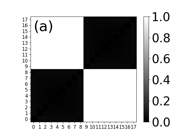
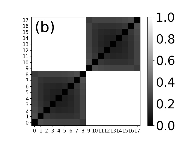
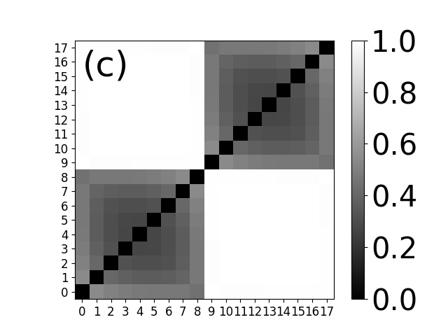
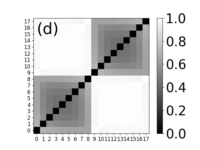
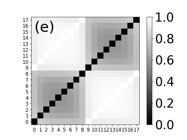
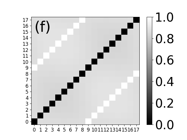
Figure 1: (a)-(f) Distance matrices obtained from numerical computation for interaction strengths $V=0.1$ (a), $V=1$ (b), $V=2$ (c), $V=3$ (d), $V=4$ (e) and $V=12$ (f).

VII.2 Distances from $k=-\pi$

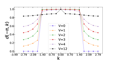
Figure 2: Distance $d(-\pi,k)$ between $k=-\pi$ and the other $k$ modes in the Brillouin zone (BZ) for different values of the interaction strength $V$.

Figure (2) shows the distance, $d(-\pi,k)$ for different interaction strengths. The Fermi points are $k_{F}=\pm\pi/2$. At $V=0$, the distance jumps from 0 to 1 across the Fermi points. At small $V$, the discontinuity seems to persist and at large $V$, there is no discontinuity.

We examine this more closely by plotting $\delta$ which is the difference between $d(-\pi,-\frac{\pi}{2})$ and $d(-\pi,-\frac{\pi}{2}-\frac{2\pi}{L})$ for different system sizes in Fig. (3). The discontinuity is insensitive to the system size for $V\lessapprox 2$ and starts depending on the system size for larger values of $V$ indicating that the discontinuity may persist in the thermodynamic limit at small values of $V$. However, at $L=18$, we are far from the thermodynamic limit. While it seems clear that there is a very sharp change across the Fermi point, we cannot conclusively say if it is a discontinuity. The thermodynamic limit is accessible at small $V$ by the bosonisation technique. We are currently investigating this and will be reporting it in a future publication.

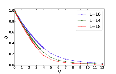
Figure 3: $\delta=d(-\pi,-\dfrac{\pi}{2})-d(-\pi,-\dfrac{\pi}{2}-\dfrac{2\pi}{L})$, gives a measure of the discontinuity across the Fermi points. It is studied as a function of interaction strength $V$ for different system sizes.

An interesting feature in Fig. (2) is that $d(-\pi,0)=1$ for all values of the interaction. Indeed we find that $d(k,k+\pi)=1$ for all values of $k$ and $V$. From Eq. (50) it can be inferred that this is a consequence of the particle-hole symmetry of the model, $C^{\dagger}_{k}\rightarrow C_{k+\pi}$.

VII.3 Nearest neighbour distances

We find that the distances between two quasi-momenta do not decrease monotonically with the separation between them. The $V=\infty$ case is an extreme example, however, as shown in Fig. (4) this is true even for a small value of $V$. At $V=1$, we find for the distances from a reference $k$ mode $-\pi/2$ ($k_{ref}$), the distance from the closest $k$ mode is infact having the optimum value. This indicates that the quantum metric $g(k)$, defined by $\lim_{\Delta k\rightarrow 0}d^{2}(k,k+\Delta k)=g(k)\Delta k^{2}$, may not be well defined in this system.

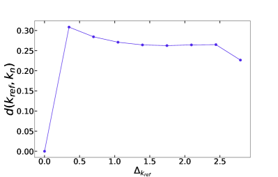
Figure 4: Distances between $k_{ref}=-\dfrac{\pi}{2}$ and other modes $k_{n}$, where $k_{n}\in FS$, as a function of $\Delta_{k_{ref}}$, which is the seperation between them in the BZ given by $\Delta_{k_{ref}}=k_{n}-k_{ref}$, for $V=1$.

The nearest neighbour distance $d(k_{n},k_{n+1})$ is plotted for different $V$ in Fig. (5) over half the Brillioun zone, over the full BZ the value of $n$ runs from $0$ ($k_{0}\equiv-\pi$) to $L-1$ ($k_{L-1}\equiv\pi-\frac{2\pi}{L}$) and we consider $k_{L}\equiv-\pi$. At $V=0$ there are all zeros except at the Fermi point, when one quasi-momentum is in the Fermi sea and it’s nearest neighbour is outside it, in which case it is equal to 1. Hence there is a delta function singularity at the Fermi point. At low $V$ this singularity remains but gets smoothened out at large $V$. At $V=\infty$ all the nearest neighbour distances are equal and it can be seen that this is almost the case at $V=12$.

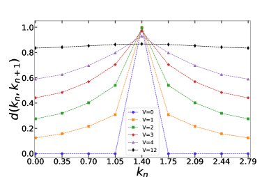
Figure 5: Nearest Neighbour Distance for different interaction strength $V$, over half the BZ.

The clustering feature discussed in Section VI.3 is nicely illustrated by the nearest neighbour distances using the following construction which represents them on a unit circle.

We first define a radius, $R$, in terms of the sum of all the nearest neighbour distances,

$$2\pi R\equiv\sum_{i=0}^{L-1}d(k_{i},k_{i+1}).$$ (66)

This radius varies with $V$, from $R=1/\pi$ at $V=0$ to $R=c(\alpha)L/(2\pi)$ at $V=\infty$.

Each nearest neighbour distance is represented by an angle,

$$\Delta\theta_{i,i+1}=\frac{d(k_{i},k_{i+1})}{R}.$$ (67)

Finally, each quasi-momentum is represented by an angle,

$$\theta_{k_{i}}=\sum_{j=0}^{i}\Delta\theta_{j-1,j}$$ (68)

where, $\Delta\theta_{-1,0}\equiv 0$.

The points on the unit circle, as defined above, are plotted in Fig. (6). At $V=0$ all the points collapse into $\theta=0,\pi$, at small $V$, they spread out but the points in the Fermi sea and those outside it are well seperated. At $V$ between 2 and 3, the seperation starts closing and at $V\geq 4$ the seperation is almost indistinguishable from the $V=\infty$ case when they are equally spaced.

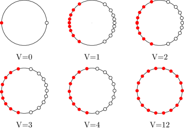
Figure 6: Schematic representations on unit circle for different interaction $V$. For each unit circle, in the first five cases ($V=0-4$), the smaller filled circles on the unit circle represent modes inside the Fermi sea and the smaller open circles correspond to modes outside the Fermi sea. For the sixth unit circle ($V=12$) all the modes are equally spaced and represented by smaller filled circles.

VII.4 Structure of triangles

We now consider the structure of the triangles corresponding to the three distances between three quasi-momenta. At $V=\infty$, most of the triangles are equilateral triangles (except those that contain $k$ and $k+\pi$). We consider only the equilateral triangles. At $V=0$, as mentioned earlier, there are no triangles, only points and segments.

The triangles are of two types, one formed of all three quasi-momenta in the Fermi sea (or all three outside it). We refer to these as particle triangles. The other type are those formed by two quasi-momenta in the Fermi sea and one outside (or the other way around). We refer to these as particle-hole triangles.

As $V$ decreases from $\infty$, we see three regimes. Up to $V\approx 4$, nothing much happens. The particle triangles then start shrinking and shrink to points at $V=0$. The particle-hole triangles change shape at $V\approx 2$ and become isosceles triangles, they then shrink to segments at $V=0$. This behaviour is illustrated in Fig. (7) and Fig. (8) respectively.

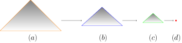
Figure 7: (Color online) $(a)-(c)$ Particle triangles for values of interaction strength $V=4$ (a) (orange), $V=2$ (b) (blue) and $V=1$ (c) (green). $V=0$ (d) (red) corresponds to a point.

Figure 8: (Color online) $(a)-(c)$ Particle-hole triangles for values of interaction strength $V=6$ (a) (purple), $V=4$ (b) (orange) and $V=2$ (c) (blue). $V=0$ (d) (red) corresponds to a segment.

VIII Discussion and conclusion

To summarise our results, we have given a definition of quantum distances between pairs of points in the spectral parameter space. We proved that our definition satisfies the triangle inequalities. The spectral parameters are completely general, they could be quasi-momenta, positons labelling Wannier orbitals, parameters labelling the eigenfunctions of some confining potential like in a quantum dot or an optical trap.

Our definition of the quantum distances is a purely kinematic one, since it is in terms of the expectation values of the exchange operators. Thus, if the state being considered is the ground state of a system, then the geometry defined is manifestly a ground state property. This is in contrast with definitions in terms of Green’s functions which is a dynamic quantity.

Because of this, our definition can be applied to any state, not necessarily the ground state. Thus, it could potentially find applications in quantum dynamical systems and provide a dynamical geometrical description.

We have applied our formalism to compute and study the distance matrix of the ground state of the one-dimensional $t-V$ model. The finite system that we are studying does not have a phase transition but only a crossover from the metallic to the insulating regime as $V$ is increased. We observe that the metallic regime is characterized by a clustering of the distances, either very small or close to 1. They also show signals of sharp Fermi points. As $V$ increases the distances spread and the Fermi points are washed out.

We have illustrated this behaviour in three ways.

• By examining the distances from a fixed point (chosen to be $k=-\pi$) to all the others. This shows very sharp changes at the Fermi points at low $V$, which smoothen out at large $V$.

• By examining the nearest neighbour distances and constructing a representation of these on a unit circle. This representation clearly shows clustering at small $V$ which gets washed out at large $V$.

• By examining the triangles formed by the distances between three quasi momenta. The triangles are of two types, both have finite areas in the insulating regime which drastically reduce in the metallic regime.

In all the three cases discussed above the crossover happens around $V=2-4$. Since previous studies Shankar (1990) have established that the metal-insulator transition occurs at $V=2$, we conclude that the “clustering-declustering” feature that we observe in the distance matrix is indeed characterizing the metal-insulator crossover.

Our work opens up many directions for further work. One direction is the following. In this paper we have shown that the distance matrix shows clear signals of the metal-insulator transition. There is a large body of mathematical literature on distance matrices and the geometry of the embedding space. So the question is, what geometric quantity constructed out of the distance matrix best describes the metal-insulator transition? We will be addressing and reporting on this issue in our following paper.

Another remaining question is the issue of defining geometric phases associated with loops in the spectral parameter space. Is it possible for general correlated states? If so, what is the definition?

IX Acknowledgements

We are grateful to R. Simon, S. Ghosh, R. Anishetty, G. Date, and A. Mishra for useful discussions.

Appendix A Reduction to the classical Ptolemy problem for $\alpha=2$

In this appendix, we will show that, for $\alpha=2$, the problem of proving the triangle inequalities, reduces to the classical Ptolemy problem in $3$-dimensional Euclidean space.

To state the problem, we are given four normalized vectors in a Hilbert space, ${\cal H}$, $|\chi_{\mu}\rangle,~{}\mu=0,\dots,3$, where, with reference to the notation in Section III.3, we have defined $|\psi\rangle\equiv|\chi_{0}\rangle$. The six distances between these four vectors are given by,

$$D_{\mu\nu}=\sqrt{1-|\langle\chi_{\mu}|\chi_{\nu}\rangle|^{2}}.$$ (69)

We will now prove that we can always find $4$ points in a $3$-dimensional Euclidean space, $\vec{x}_{\mu}$, such that,

$$D_{\mu\nu}=|\vec{x}_{\mu}-\vec{x}_{\nu}|.$$ (70)

This reduces the problem to the classical Ptolemy problem.

We can always find a $4$-dimensional subspace of ${\cal H}$ which contains the four vectors, $|\chi_{\mu}\rangle$. The physical states, forming the manifold $CP_{3}$, are in one-to-one correspondence with the pure state density matrices,

$$\rho_{\mu}\equiv|\chi_{\mu}\rangle\langle\chi_{\mu}|.$$ (71)

The distances defined in Eq. (69) can be expressed as,

$$D_{\mu\nu}=\sqrt{1-{\rm tr}\rho_{\mu}\rho_{\nu}}.$$ (72)

Since $\rho_{\mu}$ are hermitian, they can be expressed as a linear combination, with real coefficients, of the identity matrix and the $15$ generators of $SU(4)$ in the fundamental representation. We denote them by, $T_{\alpha},~{}\alpha=1,\dots,15$. They can always be chosen such that,

$${\rm tr}T_{\alpha}=0,~{}~{}~{}~{}~{}~{}{\rm tr}T_{\alpha}T_{\beta}=\delta_{\alpha\beta}.$$ (73)

Thus we have,

$$\rho_{\mu} = a_{0}I+\sum_{\alpha=1}^{15}a_{\mu}^{\alpha}T_{\alpha}$$ (74)

$$a_{0} = \frac{1}{4}{\rm tr}\rho_{\mu}$$ (75)

$$a_{\mu}^{\alpha} = {\rm tr}T_{\alpha}\rho_{\mu}.$$ (76)

The fact that, ${\rm tr}\rho_{\mu}^{2}={\rm tr}\rho_{\mu}=1$ implies that,

$$a_{0}=\frac{1}{4},~{}\vec{a}_{\mu}\cdot\vec{a}_{\mu}\equiv\sum_{\alpha=1}^{15}~{}a_{\mu}^{\alpha}a_{\mu}^{\alpha}=1-\frac{1}{16}=\frac{15}{16}.$$ (77)

Note that $\rho_{\mu}^{2}=\rho_{\mu}$ implies other constraints on $\vec{a}$, but these are not relevant for our proof.

Thus, we have shown that each of the physical states, $\rho_{\mu}$, can be represented by a point on a $14$-dimensional sphere of radius $\frac{\sqrt{15}}{4}$.

The distance $D_{\mu\nu}$ can be expressed in terms of $\vec{a}_{\mu}$,

$$D^{2}_{\mu\nu} = 1-{\rm tr}\rho_{\mu}\rho_{\nu}$$ (78)

$$= \frac{15}{16}-\vec{a}_{\mu}\cdot\vec{a}_{\nu}$$

$$= \frac{1}{2}|\vec{a}_{\mu}-\vec{a}_{\nu}|^{2}.$$

Thus, if we define $\vec{x}_{\mu}\equiv\frac{1}{\sqrt{2}}\vec{a}_{\mu}$, then we have constructed four points, $\vec{x}_{\mu}$, in a $15$-dimensional Euclidean space such that the $6$ distances between them are $D_{\mu\nu}$. Namely,

$$D_{\mu\nu}^{2}=|\vec{x}_{\mu}-\vec{x}_{\nu}|^{2}.$$ (79)

We can always find a $3$-dimensional subspace of this $15$-dimensional Euclidean space that contains the four points $\vec{x}_{\mu}$.

Hence, we have found $4$ points, $\vec{x}_{\mu}$ in a $3$-dimensional Euclidean vector space such that the $6$ distances between them is $D_{\mu\nu}$. The problem thus reduces to the classical Ptolemy problem.

References

- Haldane (2012) F. D. M. Haldane, “Topology and geometry in quantum condensed matter,” PCCM-PCTS Summer School, (2012).
- Resta (2011) R. Resta, The European Physical Journal B 79, 121 (2011).
- Mukunda and Simon (1993) N. Mukunda and R. Simon, Annals of Physics 228, 205 (1993).
- Sriluckshmy et al. (2014) P. V. Sriluckshmy, A. Mishra, S. R. Hassan, and R. Shankar, Phys. Rev. B 89, 045105 (2014).
- Faye et al. (2014) J. P. L. Faye, D. Sénéchal, and S. R. Hassan, Phys. Rev. B 89, 115130 (2014).
- Thouless et al. (1982) D. J. Thouless, M. Kohmoto, M. P. Nightingale, and M. den Nijs, Phys. Rev. Lett. 49, 405 (1982).
- Sundaram and Niu (1999) G. Sundaram and Q. Niu, Phys. Rev. B 59, 14915 (1999).
- Haldane (2006) F. D. M. Haldane, (2006), -Les Houches Summer School, Quantum Magnetism.
- Xiao et al. (2010) D. Xiao, M.-C. Chang, and Q. Niu, Rev. Mod. Phys. 82, 1959 (2010).
- Haldane (2004) F. D. M. Haldane, Phys. Rev. Lett. 93, 206602 (2004).
- Karplus and Luttinger (1954) R. Karplus and J. M. Luttinger, Phys. Rev. 95, 1154 (1954).
- Marzari and Vanderbilt (1997) N. Marzari and D. Vanderbilt, Phys. Rev. B 56, 12847 (1997).
- Kohn (1964) W. Kohn, Phys. Rev. 133, A171 (1964).
- Resta (1998) R. Resta, Phys. Rev. Lett. 80, 1800 (1998).
- Resta and Sorella (1999) R. Resta and S. Sorella, Phys. Rev. Lett. 82, 370 (1999).
- Souza et al. (2000) I. Souza, T. Wilkens, and R. M. Martin, Phys. Rev. B 62, 1666 (2000).
- Resta (2002) R. Resta, Journal of Physics: Condensed Matter 14, R625 (2002).
- Resta (2005) R. Resta, Phys. Rev. Lett. 95, 196805 (2005).
- Resta (2015) R. Resta, (2015), ecture Notes.
- Wang et al. (2010) Z. Wang, X.-L. Qi, and S.-C. Zhang, Phys. Rev. Lett. 105, 256803 (2010).
- Wang and Zhang (2012) Z. Wang and S.-C. Zhang, Phys. Rev. X 2, 031008 (2012).
- Wang et al. (2011) L. Wang, X. Dai, and X. C. Xie, Phys. Rev. B 84, 205116 (2011).
- Gurarie (2011) V. Gurarie, Phys. Rev. B 83, 085426 (2011).
- Chen and Lee (2011) K.-T. Chen and P. A. Lee, Phys. Rev. B 84, 205137 (2011).
- Wang et al. (2012) Z. Wang, X.-L. Qi, and S.-C. Zhang, Phys. Rev. B 85, 165126 (2012).
- Bargmann (1964) V. Bargmann, Journal of Mathematical Physics 5, 862 (1964).
- Simon and Mukunda (1993) R. Simon and N. Mukunda, Phys. Rev. Lett. 70, 880 (1993).
- Schoenberg (1940) I. J. Schoenberg, Annals of Mathematics 41, 715 (1940).
- Yang and Yang (1966) C. N. Yang and C. P. Yang, Phys. Rev. 150, 321 (1966).
- Baxter (1982) R. J. Baxter, Exactly Solved Models in Statistical Mechanics (Academic Press, 1982).
- Cazalilla et al. (2011) M. A. Cazalilla, R. Citro, T. Giamarchi, E. Orignac, and M. Rigol, Rev. Mod. Phys. 83, 1405 (2011).
- Luttinger (1963) J. M. Luttinger, Journal of Mathematical Physics 4, 1154 (1963).
- Haldane (1980) F. D. M. Haldane, Phys. Rev. Lett. 45, 1358 (1980).
- Haldane (1981) F. D. M. Haldane, Journal of Physics C: Solid State Physics 14, 2585 (1981).
- Shankar (1990) R. Shankar, International Journal of Modern Physics B 04, 2371 (1990).
- Liberti and Lavor (2016) L. Liberti and C. Lavor, International Transactions in Operational Research 23, 897 (2016).