Neutron Electric Dipole Moment from Beyond the Standard Model

Abstract:

We present an update on our calculations of the matrix elements of the CP violating quark and gluon chromo-EDM operators, as well as the operators these mix with, such as the QCD Theta-term. Their contribution to the neutron EDM is obtained by extrapolating the $F_{3}$ form factor of a vector current to zero momentum transfer. The calculation is being done using valence Wilson-clover quarks on HISQ background configurations generated by the MILC collaboration.

1 Introduction

Violation of the symmetry under simultaneous charge-conjugation and parity-flip (CP) is a core ingredient in the standard model (SM) and is necessary to explain the vast excess of matter over antimatter in the universe [1]. The SM CP-violation (CPV) is small and arises from the weak mixing between the quark [2, 3], and possibly also lepton [4, 5], families. Cosmological models require much stronger CPV [6], and most theories beyond the SM (BSM) do indeed produce it naturally. If this additional CPV is produced naturally by physics at a few TeV, the next generation of electric dipole moment (EDM) measurements [7, 8] are likely to find it, and the neutron is a very good candidate system. To connect theory to experiments, it is imperative to obtain the matrix elements (ME) of the CPV effective operators that control the EDMs of various particles. Here, we discuss our progress in calculating the neutron EDM (nEDM) due to the quark chromo-EDM operators.

1.1 BSM Operators

The SM CPV in the weak sector leads to effective dimension-6 four-fermion operators at hadronic scales. In principle, these also lead to dimension-3 CPV mass terms, $\bar{\psi}\gamma_{5}\tau\psi$, for the fermions, where $\psi$ is the fermion field and $\tau$ is a flavor matrix. Axial transformations can be used to remove the quark CPV masses, except when $\tau$ is the identity, in which case the anomaly transforms it to the dimension-4 gluon-topological-charge operator (also called the $\Theta$-term), $G_{\mu\nu}\tilde{G}^{\mu\nu}$, where $G$ is the gluon field strength [10]. Phenomenological estimates, using the limit on the neutron electric dipole moment, already constrain the total coefficient $\bar{\Theta}$ of this operator to be anomalously small, less than $3\times 10^{-10}$ [11].

In BSM theories, CPV operators start at dimension 6 at the weak scale [12], but two of them—the quark EDM (qEDM), $\bar{\psi}\tau\Sigma_{\mu\nu}\tilde{F}^{\mu\nu}\psi$, where $F$ is the electromagnetic field tensor, and the quark chromo-EDM (qCEDM), $\bar{\psi}\tau\Sigma_{\mu\nu}\tilde{G}^{\mu\nu}\psi$—become dimension 5 after electroweak symmetry breaking. This means that their natural suppression relative to the QCD scale is by $v_{\rm EW}/M^{2}_{\rm BSM}$ rather than by $1/M^{2}_{\rm BSM}$ as for the remaining dimension-6 operators—the gluon chromo-EDM (also called the Weinberg 3-gluon operator), $G_{\mu\nu}G_{\lambda\nu}\tilde{G}_{\mu\lambda}$, and various 4-fermion operators. In many BSM models, however, the dimension-5 operators come with extra Yukawa suppression, and their effect is comparable to the other dimension-6 operators. Thus, all these should be considered at the same level, and their ME within the neutron state calculated.

1.2 Form Factors

Using Lorentz symmetry, the response of a neutron to the vector current can be written in terms of the Dirac $F_{1}$, Pauli $F_{2}$, anapole $F_{A}$, and electric-dipole $F_{3}$ form-factors as

$$\langle N|V_{\mu}(q)|N\rangle = \overline{u}_{N}\left[\gamma_{\mu}\;F_{1}(q^{2})+i\frac{[\gamma_{\mu},\gamma_{\nu}]}{2}q_{\nu}\;\frac{F_{2}(q^{2})}{2m_{N}}+{(2i\,m_{N}\gamma_{5}q_{\mu}-\gamma_{\mu}\gamma_{5}q^{2})\;\frac{F_{A}(q^{2})}{m_{N}^{2}}}\right.$$

$$\qquad\qquad\qquad\qquad\qquad\qquad\qquad\qquad\qquad\left.{}+{\frac{[\gamma_{\mu},\gamma_{\nu}]}{2}q_{\nu}\gamma_{5}\;\frac{F_{3}(q^{2})}{2m_{N}}}\right]u_{N}\,,$$

in the Euclidean metric. Here $V_{\mu}$ represents the electromagnetic vector current, $u_{N}$ represents the neutron spinor normalized such that $u_{N}\bar{u}_{N}=-i\not{p}+m_{N}$, where $p$ is its momentum and $m_{N}$ its mass, $q$ the momentum inserted by the vector current $V_{\mu}$, and $|N\rangle$ is the neutron state. The Sachs form factors [13, 14, 15] that describe the charge and current densities in the Breit frame, are related to these as $G_{E}\equiv F_{1}-(q^{2}/4M^{2})F_{2}$ and $G_{M}\equiv F_{1}+F_{2}$. The electric charge is $G_{E}(0)=F_{1}(0)=0$ and the anomalous magnetic dipole moment is $G_{M}(0)/2M_{N}=F_{2}(0)/2M_{N}$. The anapole moment breaks the symmetry under simultaneous parity-flip and time-reversal (PT), and so, will be zero in our calculations. The electric dipole moment is given by the CP-violation form factor $F_{3}$ at zero $q^{2}$, $d_{E}=F_{3}(0)/2m_{N}$.

If parity is violated, an operator that creates an asymptotic neutron with the standard parity transformation properties is $N_{\alpha_{N}}\equiv\epsilon_{abc}\left[(\bar{d}^{a})^{C}\gamma_{5}Pu^{b}\right]\exp{\{i\alpha_{N}\gamma_{5}\}}d^{c}$, where $a$, $b$, and $c$ are color labels, the superscript $C$ represents charge conjugation, $P\equiv(1+\gamma_{4})/2$ is positive-energy projector for zero-momentum quarks that improves the signal, and $\alpha_{N}$ is a constant depending on the asymptotic state that needs to be determined. Under the standard choice of quark and neutron parities, $\alpha_{N}$ is real when PT is a good symmetry, imaginary when CP is good, and zero if parity is unbroken.

2 Status of Lattice Calculations and Preliminary Results

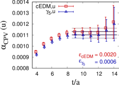
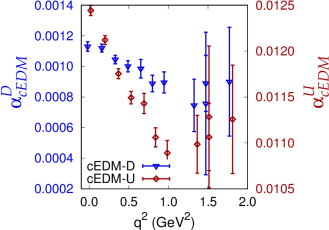
(a)	(c)
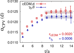
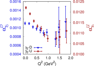
(b)	(d)

Figure 1: (a) The extraction of $\alpha_{N}$ with the insertion of the chromo-EDM (labeled cEDM) or CPV mass (labeled $\gamma_{5}$) operators on $u$ quarks. (b) Same as (a), but with the insertion on the $d$ quark. (c) $\alpha_{N}$ due to chromo-EDM insertion as a function of the 3-momentum of the neutron; the insertions on the $u$ and $d$ quarks are shown separately. (d) Same as (c), but for the CPV mass term.

We have recently completed an analysis of the proton and neutron EDMs arising from the quark EDM [16]. Here we report on progress on nucleon EDMs arising from the quark chromo-EDM operator. This operator has power divergent mixing with lower dimensional pseudoscalar quark mass term and the gluon topological charge (if chiral symmetry is violated) that has to be controlled. We, therefore, discuss these operators as well.

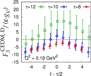
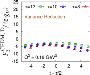
(a)	(b)
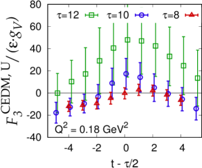
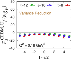
(c)	(d)

Figure 2: $F_{3}/(\varepsilon\cdot g_{V})$ for the neutron due to chromo-EDM insertion on the $d$ ((a) and (b)) and $u$ ((c) and (d)) quarks before ((a) and (c)) and after ((b) and (d)) variance reduction. Here $\varepsilon$ is the coefficient of the CP-violating term, and the baryonic vector charge $g_{V}$ is unity in the continuum limit and cancels the lattice renormalization of the vector current.

The quark chromo-EDM operator is a quark bilinear, so its ME can be calculated using the Schwinger source method as described in previous proceedings [17, 18]. All the calculations presented here were done with Clover fermions on a MILC generated $L^{3}\times T=24^{3}\times 64$ HISQ ensemble [19, 20] with lattice spacing $a=0.1207(11)~{}\mbox{fm}$ and pion mass $M_{\pi}^{\rm sea}=305.3(4)~{}\mbox{MeV}$. The parameters of the Wilson-clover action used are $\kappa\approx 0.1272103$ corresponding to $M_{\pi}^{\rm val}=310.2(2.8)~{}\mbox{MeV}$ and $c_{\rm SW}=1.05094$ determined using tree-level boosted perturbation theory with $u_{P}^{HYP}=0.9358574(29)$. Statistical precision is increased using the truncated solver method [21, 22] with 128 low-precision and 4 high-precision measurements on each of the 1012 configuration. The quark-disconnected diagrams were ignored in all of the reported calculations.

To determine $\alpha_{N}$, we use $\Im\mathop{\rm Tr}\gamma_{5}\langle N_{0}\bar{N}_{0}\rangle/\Re\mathop{\rm Tr}\langle N_{0}\bar{N}_{0}\rangle$, where $\langle N_{0}\bar{N}_{0}\rangle$ is the propagator with $\alpha_{N}=0$. Asymptotically, this gives $-2\tan\alpha_{N}$. Figures 1(a) and (b) show $\alpha_{N}$ extracted from the neutron propagator for the CP violation parameter $\varepsilon$ in the small (linear) regime [17]. Figures 1(c) and (d) show that there is a strong dependence of the extracted $\alpha_{N}$ on the momentum of the neutron, probably due to lattice spacing artifacts.

       

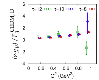
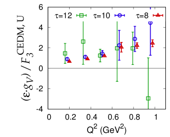
Figure 3: $(\varepsilon\cdot g_{V})/F_{3}$ versus $Q^{2}$ for the neutron with chromo-EDM insertion on the $d$ (left) and $u$ (right) quarks at various source-sink separations.

The three point function, from which the ME of $V_{\mu}$ are extracted, calculated is

$$\langle\Omega|{N_{0}(\vec{0},0)V_{\mu}(\vec{q},t)\overline{N_{0}}(\vec{p},T)}|\Omega\rangle = \sum_{n,n^{\prime}}e^{-i\alpha_{n}\gamma_{5}}u_{n}e^{-m_{n}t}\;{\langle n|V_{\mu}(q)|n^{\prime}\rangle}\;e^{-E_{n^{\prime}}(T-t)}{\overline{u}}_{n^{\prime}}e^{-i\alpha_{n^{\prime}}^{*}\gamma_{5}}$$

with projection onto only one spinor component using ${\cal P}\equiv\frac{1}{2}(1+\gamma_{4})(1+i\gamma_{5}\gamma_{3})$. The ME is isolated using the combination

$$R^{\mu}\equiv\frac{C_{\rm 3pt}^{\mu}(q;\tau,t)}{C_{\rm 2pt}(\tau;0)}\sqrt{\frac{C_{\rm 2pt}(t;0)C_{\rm 2pt}(\tau;0)C_{\rm 2pt}(\tau-t;-q)}{C_{\rm 2pt}(t;-q)C_{\rm 2pt}(\tau;-q)C_{\rm 2pt}(\tau-t;0)}}\,$$

where $C_{\rm 3pt}^{\mu}$ are the projected 3pt functions and $C_{\rm 2pt}$ are the real parts of projected 2pt functions. The eight quantities—$\Re R^{\mu}$ and $\Im R^{\mu}$—provide an overdetermined set from which the three form factors can be extracted. In fact, these break up into two sets of four quantities: the components $V_{R}\equiv(\Re\vec{R},i\Im R^{4})$ give $G_{2}\equiv G_{E}+\tan\alpha_{N}(Q^{2}/4m_{N}^{2})F_{3}$, whereas the other four components $V_{I}\equiv(\Im\vec{R},-i\Re R^{4})$ give $G_{1}\equiv G_{M}$ and $G_{3}\equiv F_{3}+\tan\alpha_{N}F_{2}$. The overdetermined set of equations for the transition ME between a neutron at rest and momentum $(-\vec{q},E_{N})$ is

$$E\equiv\begin{pmatrix}X_{1}&0&X_{3}\\ 0&Y_{1}&0\end{pmatrix}\begin{pmatrix}G_{1}\\ G_{2}\\ G_{3}\end{pmatrix}-\begin{pmatrix}V_{R}\\ V_{I}\end{pmatrix}=0\,,$$

where $X_{1}\equiv m(-cq_{2},cq_{1},s(E_{N}-m_{N}),-isq_{3})^{T}$, $Y_{1}\equiv m_{N}c(q_{1},q_{2},q_{3},-i(E_{N}+m_{N}))^{T}$, $X_{2}\equiv-(q_{3}/2m_{N})Y_{1}$, $c\equiv\cos^{2}\alpha_{N}$ and $s\equiv\sin\alpha_{N}\cos\alpha_{N}$. We solve this set by the method of least squares, i.e., we solve the linear equations obtained by differentiating $E^{T}WE$ with respect to $G_{i}$ for a positive weight matrix $W$, which we choose, for simplicity, to be $\mathop{\rm diag}(\sigma_{R}^{2},\sigma_{I}^{2})^{-1}$, where $\sigma_{R}$ and $\sigma_{I}$ are the errors on $V_{R}$ and $V_{I}$ respectively.

Figure 2 (a) and (c) show that the signal in the $F_{3}^{u}$ and $F_{3}^{d}$ is, a priori, poor. To improve the signal, we propose the following variance reduction method: use quantities $z_{i}$ that are correlated with $F_{3}$ and have zero expectation value, and construct the lower variance estimator $F_{3}-\sigma^{2}_{Fi}\Sigma^{-2}_{ij}z_{j}$, where $\Sigma^{-2}$ is the inverse variance-covariance matrix of $z_{i}$ and $\sigma^{2}_{Fi}$ is the covariance of $F_{3}$ with $z_{i}$. Since we know that for $\varepsilon=0$ (CP-symmetric case), $F_{3}$ is zero even at finite $a$ and for our mixed action calculation, and remains highly correlated with $F_{3}$ for small $\varepsilon$, we expect using $F_{3}(\varepsilon=0)$ as a $z_{i}$ in the above expression will reduce the variance. Figures 2 (b) and (d) show that this variance reduction method improves the signal substantially.

Figure 3 shows that $1/F_{3}$ behaves linearly with $Q^{2}$ as would be expected from pole-dominance. Also, the dependence on the source-sink separation $\tau$ is small, indicating excited state contributions are manageable. The next important step, once the signal is established, is to subtract power divergences in the renormalization due to operator mixing to ensure a finite result in the continuum limit.

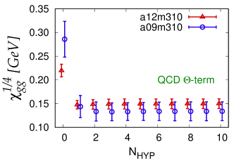
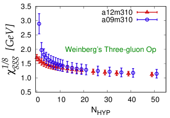
Figure 4: The evolution of the susceptibilities of the topological charge (left) and the Weinberg operator (right) as a function of the HYP smearing steps.

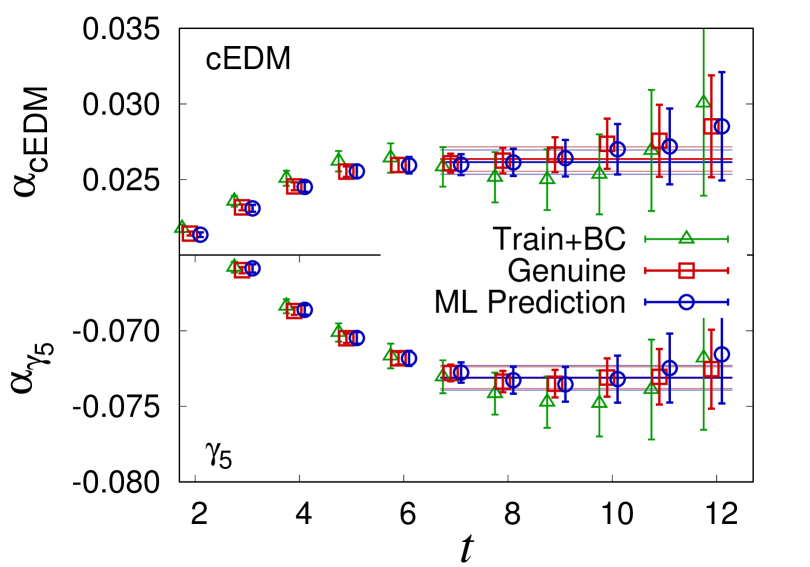
Figure 5: Comparison of the predicted and calculated imaginary part of the propagator with the insertion of the chromo-EDM and CPV mass term from the real part of the propagator with no insertion. Note that the final errors on the prediction are comparable to the actual errors, substantially reduced from the errors on the train set. These results are obtained using the choice of $\varepsilon_{\textrm{cEDM}}=0.004$ and $\varepsilon_{\gamma_{5}}=-0.004$.

3 Ongoing Work

We are extending the calculation of the chromo-EDM by constructing various combinations of the matrix elements that each provide an estimate of $F_{3}$, and by adding the contribution of the disconnected diagrams. To address divergent mixing under renormalization, the RI-sMOM scheme defined in [10] is complicated, so we are evaluating gradient-flow regularization [23]. We will first implement this scheme for the simpler case of the two gluonic operators. In Figure 4, we show the evolution of the susceptility of the scale-dependent Weinberg operator with the number of HYP smearings and compare it to the scale-independent topological susceptibility. We are investigating whether the expected scale-dependence persists under gradient-flow smearing. The motivation is that under gradient flow renormalization, the Weinberg operator needs no divergent subtraction. The next step will be to extend this to the fermion sector. To demonstrate efficacy, we will first compare results for isovector charges renormalized using the RI-sMOM scheme and gradient flow.

Finally, we are developing machine learning algorithms to reduce the computational effort. Building on the similarity to reweighting ensembles or unraveling quantum trajectories, the method proceeds by finding a combination of easily calculated and statistically precise quantities that have a high correlation with more compute-intensive quantities of interest, and then making the estimates rigorous by implementing standard bias reduction techniques. Initial tests of these ideas show promise as illustrated in Figure 5.

We acknowledge computer resources provided by LANL (IC), NERSC (US DOE contract DE-AC02-05CH11231), OLCF (US DOE contract DE-AC05-00OR22725) and JLAB (USQCD); the CHROMA software suite [24]; and support from US DOE contract DE-AC52-06NA25396 and LANL LDRD grant 20190041DR.

References

- [1] Sakharov, A. D. Soviet Physics Uspekhi 34(5), 392 (1991).
- [2] Cabibbo, N. Physical Review Letters 10, 531–533 (1963).
- [3] Kobayashi, M. and Maskawa, T. Progress of Theoretical Physics 49, 652–657 (1973).
- [4] Pontecorvo, B. Sov. Phys. JETP 7, 172–173 (1958). [Zh. Eksp. Teor. Fiz.34,247(1957)].
- [5] Maki, Z., et al. Progress of Theoretical Physics 28, 870–880 (1962).
- [6] Trodden, M. Rev. Mod. Phys. 71, 1463–1500 (1999).
- [7] Semertzidis, Y. K. In Journal of Physics Conference Series, volume 335 of Journal of Physics Conference Series, 012012, (2011).
- [8] Chupp, T., et al. arXiv:1710.02504 [physics.atom-ph] (2017).
- [9] Xing, Z.-z. and Zhou, Y.-L. Phys. Rev. D 88, 033002 (2013).
- [10] Bhattacharya, T., et al. Phys. Rev. D 92, 114026 (2015).
- [11] Pospelov, M. and Ritz, A. Nuclear Physics B 573(1), 177 – 200 (2000).
- [12] Pospelov, M. and Ritz, A. Annals of Physics 318(1), 119 – 169 (2005). Special Issue.
- [13] Ernst, F. J., et al. Phys. Rev. 119, 1105–1114 (1960).
- [14] Barnes, K. Physics Letters 1(5), 166 – 168 (1962).
- [15] Hand, L. N., et al. Rev. Mod. Phys. 35, 335 (1963).
- [16] Gupta, R., et al. Phys. Rev. D 98, 091501 (2018).
- [17] Bhattacharya, T., et al. PoS LATTICE2016, 225 (2016).
- [18] Yoon, Boram, et al. EPJ Web Conf. 175, 01014 (2018).
- [19] Follana, E., et al. Phys. Rev. D 75, 054502 (2007).
- [20] Bazavov, A., et al. Phys. Rev. D 87, 054505 (2013).
- [21] Bali, G. S., et al. Computer Physics Communications 181(9), 1570 – 1583 (2010).
- [22] Blum, T., et al. Phys. Rev. D 88, 094503 (2013).
- [23] Lüscher, M. Journal of High Energy Physics 2010(8), 71 (2010).
- [24] Edwards, R. G. and Joó, B. Nuclear Physics B - Proceedings Supplements 140, 832 – 834 (2005). LATTICE 2004.