High-dimensional consistent independence testing with maxima of rank correlations

Abstract

Testing mutual independence for high-dimensional observations is a fundamental statistical challenge. Popular tests based on linear and simple rank correlations are known to be incapable of detecting non-linear, non-monotone relationships, calling for methods that can account for such dependences. To address this challenge, we propose a family of tests that are constructed using maxima of pairwise rank correlations that permit consistent assessment of pairwise independence. Built upon a newly developed Cramér-type moderate deviation theorem for degenerate U-statistics, our results cover a variety of rank correlations including Hoeffding’s $D$, Blum–Kiefer–Rosenblatt’s $R$, and Bergsma–Dassios–Yanagimoto’s $\tau^{*}$. The proposed tests are distribution-free in the class of multivariate distributions with continuous margins, implementable without the need for permutation, and are shown to be rate-optimal against sparse alternatives under the Gaussian copula model. As a by-product of the study, we reveal an identity between the aforementioned three rank correlation statistics, and hence make a step towards proving a conjecture of Bergsma and Dassios.

Keywords: Degenerate U-statistics, extreme value distribution, independence testing, maximum-type tests, rank statistics, rate-optimality.

1 Introduction

Let $\bm{X}=(X_{1},\ldots,X_{p})^{\top}$ be a random vector taking values in ${\mathbb{R}}^{p}$ and having all univariate marginal distributions continuous. This paper is concerned with testing the null hypothesis

$$H_{0}:X_{1},\ldots,X_{p}\text{ are mutually independent},$$ (1.1)

based on $n$ independent realizations $\bm{X}_{1},\ldots,\bm{X}_{n}$ of $\bm{X}$. Testing $H_{0}$ is a core problem in multivariate statistics that has attracted the attention of statisticians for decades; see e.g. the exposition in Anderson, (2003, Chap. 9) or Muirhead, (1982, Chap. 11). Traditional methods such as the likelihood ratio test, Roy’s largest root test (Roy,, 1957), and Nagao’s $L_{2}$-type test (Nagao,, 1973) target the case where the dimension $p$ is small and perform poorly when $p$ is comparable to or even larger than $n$. A line of recent work seeks to address this issue and develops tests that are suitable for modern applications involving data with large dimension $p$. This high-dimensional regime is in the focus of our work, which develops distribution theory based on asymptotic regimes where $p=p_{n}$ increases to infinity with $n$.

Many tests of independence in high dimensions have been proposed recently. For example, Bai et al., (2009) and Jiang and Yang, (2013) derived corrected likelihood ratio tests for Gaussian data. Using covariance/correlation statistics such as Pearson’s $r$, Spearman’s $\rho$, and Kendall’s $\tau$, Bao et al., (2012), Gao et al., (2017), Han et al., (2018), and Bao, (2019) proposed revised versions of Roy’s largest root test. Schott, (2005) and Leung and Drton, (2018) derived corrected Nagao’s $L_{2}$-type tests. Finally, Jiang, (2004), Zhou, (2007), and Han et al., (2017) proposed tests using the magnitude of the largest pairwise correlation statistics. Subsequently we shall refer to tests of this latter type as maximum-type tests.

The aforementioned approaches are largely built on linear and simple rank correlations. These, however, are incapable of detecting more complicated non-linear, non-monotone dependences as Hoeffding, (1948) noted in his seminal paper. Recent work thus proposed the use of consistent rank (Bergsma and Dassios,, 2014), kernel-based (Gretton et al.,, 2008; Pfister et al.,, 2018), and distance covariance/correlation statistics (Székely et al.,, 2007). However, much less is known about high-dimensional tests of $H_{0}$ that use these more involved statistics. Notable exceptions include Leung and Drton, (2018) and Yao et al., (2018). There, the authors combined Nagao’s $L_{2}$-type methods with rank and distance covariance statistics that in a tour de force are shown to weakly converge to a Gaussian limit under the null. In addition, Yao et al., (2018) proved that an infeasible version of their test is rate-optimal against a Gaussian dense alternative (Gaussian distribution with equal correlation), while still little is known about optimality of Leung and Drton’s.

In this paper, we derive maximum-type tests that are counterparts of Leung–Drton and Yao–Zhang–Shao $L_{2}$-type ones. As noted in Han et al., (2017), Leung and Drton, (2018), and Yao et al., (2018), maximum-type tests will be more sensitive to strong but sparse dependence. Designed to assess pairwise independence consistently, our tests are formed using statistics based on pairwise rank correlation measures such as Hoeffding’s $D$ (Hoeffding,, 1948), Blum–Kiefer–Rosenblatt’s $R$ (Blum et al.,, 1961), and Bergsma–Dassios–Yanagimoto’s $\tau^{*}$ (Bergsma and Dassios,, 2014; Yanagimoto,, 1970). In particular, assuming the pair of random variables $X_{i}$ and $X_{j}$ to have a joint distribution that is not only continuous but also absolutely continuous, these measures all satisfy the following three desirable properties summarized in Weihs et al., (2018):

I-consistency.

If $X_{i}$ and $X_{j}$ are independent, the correlation measure is zero.

D-consistency.

If $X_{i}$ and $X_{j}$ are dependent, the correlation measure is nonzero.

Monotonic invariance.

The correlation measure is invariant to monotone transformations.

We remark that invariance under invertible (and not just monotonic) transformations was considered in work on self-equitable measures of dependence (Kinney and Atwal,, 2014). This leads to notions of mutual information whose estimates are different from and usually more challenging to handle than the rank correlation measures we consider here; see Berrett and Samworth, (2019) and references therein. Indeed, as we shall review in Section 2, the aforementioned correlation measures are naturally estimated via U-statistics, which despite being degenerate have important special properties.

The contributions of our work are threefold. First, we prove that all the maximum-type test statistics proposed in Section 3 have a null distribution that converges to a (non-standard) Gumbel distribution under high-dimensional asymptotics. This is in contrast to the results in Han et al., (2017), where those rank correlation measures that permit consistent assessment of pairwise independence are excluded from the analysis. This exclusion is due to the lack of necessary probability tools like Cramér-type moderate deviation bounds for degenerate U-statistics, which are newly developed in this paper. Additionally, no distributional assumption except for marginal continuity is required for this result, and the parameters for the Gumbel limit can be explicitly given. This allows one to avoid permutation analysis in problems of larger scale. Second, we conduct a power analysis and give explicit conditions on a sparse local alternative under which our proposed tests have power tending to one. Third, we show that the maximum-type tests based on Hoeffding’s $D$, Blum–Kiefer–Rosenblatt’s $R$, and Bergsma–Dassios–Yanagimoto’s $\tau^{*}$ are all rate-optimal in the class of Gaussian (copula) distributions with sparse and strong dependence as characterized in the power analysis. To our knowledge this is the first rate-optimality result for a feasible test that permits consistent assessment of pairwise independence. These results are developed in Section 4. The theoretical advantages of our tests are highlighted in simulation studies (Section 5). Lastly, we note that, as an interesting by-product of the study, we give an identity among the above three statistics that helps make a step towards proving Bergsma–Dassios’s conjecture about general D-consistency of $\tau^{*}$. This observation, along with other discussions, is given in Section 6. All proofs and additional simulation results are deferred to a supplement.

Notation

The sets of real, integer, and positive integer numbers are denoted ${\mathbb{R}}$, ${\mathbb{Z}}$, and ${\mathbb{Z}}^{+}$, respectively. The cardinality of a set $\mathcal{A}$ is written $\#\mathcal{A}$. For $m\in{\mathbb{Z}}^{+}$, we define $[m]=\{1,2,\ldots,m\}$ and write $\mathcal{P}_{m}$ for the set of all $m!$ permutations of $[m]$. Let $\bm{v}=(v_{1},\ldots,v_{p})^{\top}\in{\mathbb{R}}^{p}$, $\mathbf{M}=[\mathbf{M}_{jk}]\in{\mathbb{R}}^{p\times p}$, and $I,J$ be two subsets of $[p]$. Then $\bm{v}_{I}$ is the sub-vector of $\bm{v}$ with entries indexed by $I$, i.e., $\bm{v}_{I}=(v_{i_{1}},v_{i_{2}},\ldots,v_{i_{\#I}})^{\top}$ with $i_{1}<i_{2}<\cdots<i_{\#I}$ and $\{i_{1},\ldots,i_{\#I}\}=I$. Both $\mathbf{M}_{I,J}$ and $\mathbf{M}[I,J]$ are used to refer to the sub-matrix of $\mathbf{M}$ with rows indexed by $I$ and columns indexed by $J$. The matrix ${\rm diag}(\mathbf{M})\in{\mathbb{R}}^{p\times p}$ is the diagonal matrix whose diagonal is the same as that of $\mathbf{M}$. We write $\mathbf{I}_{p}$ and $\mathbf{J}_{p}$ for the identity matrix and all-ones matrix in ${\mathbb{R}}^{p\times p}$, respectively. For a function $f:\mathcal{X}\to{\mathbb{R}}$, we define $\|f\|_{\infty}:=\max_{x\in\mathcal{X}}|f(x)|$. The greatest integer less than or equal to $x\in{\mathbb{R}}$ is denoted by $\lfloor x\rfloor$. The symbol $\mathds{1}(\cdot)$ is used for indicator functions. For any two real sequences $\{a_{n}\}$ and $\{b_{n}\}$, we write $a_{n}\lesssim b_{n}$, $a_{n}=O(b_{n})$, or equivalently $b_{n}\gtrsim a_{n}$, if there exists $C>0$ such that $|a_{n}|\leq C|b_{n}|$ for any large enough $n$. We write $a_{n}\asymp b_{n}$ if both $a_{n}\lesssim b_{n}$ and $a_{n}\gtrsim b_{n}$ hold. Write $a_{n}=o(b_{n})$ if for any $c>0$, $|a_{n}|\leq c|b_{n}|$ holds for any large enough $n$. Throughout, $c$ and $C$ refer to positive absolute constants whose values may differ in different parts of the paper.

2 Rank correlations and degenerate U-statistics

This section introduces the pairwise rank correlations that will later be aggregated in a maximum-type test of the independence hypothesis in (1.1). We present these correlations in a general U-statistic framework. In the sequel, unless otherwise stated, the random vector $\bm{X}$ is assumed to have continuous margins, that is, its marginal distributions are continuous, though not necessarily absolutely continuous.

Let $\bm{X}_{1},\dots,\bm{X}_{n}$ be independent copies of $\bm{X}$, with $\bm{X}_{i}=(X_{i,1},\dots,X_{i,p})^{\top}$. Let $j\neq k\in[p]$, and let $h:({\mathbb{R}}^{2})^{m}\to{\mathbb{R}}$ be a fixed kernel of order $m$. The kernel $h$ defines a U-statistic of order $m$:

$$\widehat{U}_{jk}=\Bigl{(}\mkern 1.0mu\begin{array}[]{@{}c@{}}n\\ m\end{array}\mkern 1.0mu\Bigr{)}^{-1}\sum_{1\leq i_{1}<i_{2}<\cdots<i_{m}\leq n}h\Big{\{}\Big{(}\begin{matrix}X_{i_{1},j}\\ X_{i_{1},k}\end{matrix}\Big{)},\ldots,\Big{(}\begin{matrix}X_{i_{m},j}\\ X_{i_{m},k}\end{matrix}\Big{)}\Big{\}}.$$ (2.3)

For our purposes $h$ may always be assumed to be symmetric, i.e., $h(\bm{z}_{1},\ldots,\bm{z}_{m})=h(\bm{z}_{\sigma(1)},\ldots,\bm{z}_{\sigma(m)})$ for all permutations $\sigma\in\mathcal{P}_{m}$ and $\bm{z}_{1},\ldots,\bm{z}_{m}\in{\mathbb{R}}^{2}$. Letting $\bm{z}_{i}=(z_{i,1},z_{i,2})^{\top}$, if both vectors $(z_{1,1},\ldots,z_{m,1})$ and $(z_{1,2},\ldots,z_{m,2})$ are free of ties, i.e., have marginal distinct entries, then we have well-defined vectors of ranks $(r_{1,1},\ldots,r_{m,1})$ and $(r_{1,2},\ldots,r_{m,2})$, and we define $\bm{r}_{i}=(r_{i,1},r_{i,2})^{\top}$ for $1\leq i\leq n$. Now a kernel is rank-based if

$$h(\bm{z}_{1},\ldots,\bm{z}_{m})=h(\bm{r}_{1},\ldots,\bm{r}_{m})$$

for all $\bm{z}_{1},\ldots,\bm{z}_{m}\in{\mathbb{R}}^{2}$ with $(z_{1,1},\ldots,z_{m,1})$ and $(z_{1,2},\ldots,z_{m,2})$ free of ties. In this case, we also say that the “correlation” statistic $\widehat{U}_{jk}$ as well as the corresponding “correlation measure” ${\mathbb{E}}\widehat{U}_{jk}$ is rank-based.

Rank-based statistics have many appealing properties with regard to independence. The following three will be of particular importance for us. Proofs can be found in, e.g., Chapter 31 in Kendall and Stuart, (1979), Lemma C4 in the supplement of Han et al., (2017), and Lemma 2.1 in Leung and Drton, (2018). We also note that, in finite samples, the statistics $\{\widehat{U}_{jk};j<k\}$ are generally not mutually independent.

Proposition 2.1.

Under the null hypothesis in (1.1) and assuming continuous margins, we have:

1. The rank statistics $\{\widehat{U}_{jk},j\neq k\}$ are all identically distributed and are distribution-free, i.e., the distribution of $\widehat{U}_{jk}$ does not depend on the marginal distributions of $X_{1},\ldots,X_{p}$;

2. Fix any $j\in[p]$, then the rank statistics $\{\widehat{U}_{jk},k\neq j\}$, are mutually independent;

3. For any $j\neq k\in[p]$, the rank statistic $\widehat{U}_{jk}$ is independent of $\{\widehat{U}_{j^{\prime}k^{\prime}};j^{\prime},k^{\prime}\not\in\{j,k\},j^{\prime}\neq k^{\prime}\}$.

Our focus will be on those rank-based correlation statistics and the corresponding measures that are induced by the kernel $h(\cdot)$ and are both I- and D-consistent. The kernels of these measures satisfy important additional properties that we will assume in our general treatment. Further concepts concerning U-statistics are needed to state this assumption. For any kernel $h(\cdot)$, any number $\ell\in[m]$, and any measure ${\mathbb{P}}_{\bm{Z}}$, we write

$$h_{\ell}(\bm{z}_{1}\ldots,\bm{z}_{\ell};{\mathbb{P}}_{\bm{Z}}):={\mathbb{E}}h(\bm{z}_{1}\ldots,\bm{z}_{\ell},\bm{Z}_{\ell+1},\ldots,\bm{Z}_{m})$$

and

$$h^{(\ell)}(\bm{z}_{1},\ldots,\bm{z}_{\ell};{\mathbb{P}}_{\bm{Z}}):=$$ (2.4)

$$~{}~{}~{}h_{\ell}(\bm{z}_{1},\ldots,\bm{z}_{\ell};{\mathbb{P}}_{\bm{Z}})-{\mathbb{E}}h-\sum_{k=1}^{\ell-1}\sum_{1\leq i_{1}<\cdots<i_{k}\leq\ell}h^{(k)}(\bm{z}_{i_{1}},\ldots,\bm{z}_{i_{k}};{\mathbb{P}}_{\bm{Z}}),$$

where $\bm{Z}_{1},\ldots,\bm{Z}_{m}$ are $m$ independent random vectors with distribution ${\mathbb{P}}_{\bm{Z}}$ and ${\mathbb{E}}h:={\mathbb{E}}h(\bm{Z}_{1},\ldots,\bm{Z}_{m})$. The kernel as well as the corresponding U-statistic is degenerate under ${\mathbb{P}}_{\bm{Z}}$ if $h_{1}(\cdot)$ has variance zero. We use the term completely degenerate to indicate that the variances of $h_{1}(\cdot),\ldots,h_{m-1}(\cdot)$ are all zero. Finally, let ${\mathbb{P}}_{0}$ be the uniform distribution on $[0,1]$, and write ${\mathbb{P}}_{0}\otimes{\mathbb{P}}_{0}$ for its product measure, the uniform distribution on $[0,1]^{2}$. Note that by Proposition 2.1(i), the study of $\widehat{U}_{jk}$ under independent continuous margins $X_{j}$ and $X_{k}$ can be reduced to the case with $(X_{j},X_{k})^{\top}\sim{\mathbb{P}}_{0}\otimes{\mathbb{P}}_{0}$.

Assumption 2.1.

The kernel $h$ is rank-based, symmetric, and has the following three properties:

1. $h$ is bounded.

2. $h$ is mean-zero and degenerate under independent continuous margins, i.e., ${\mathbb{E}}\{h_{1}(\bm{Z}_{1};{\mathbb{P}}_{0}\otimes{\mathbb{P}}_{0})\}^{2}=0$ as $\bm{Z}_{1}\sim{\mathbb{P}}_{0}\otimes{\mathbb{P}}_{0}$.

3. $h_{2}(\bm{z}_{1},\bm{z}_{2};{\mathbb{P}}_{0}\otimes{\mathbb{P}}_{0})$ has uniformly bounded eigenfunctions, that is, it admits the expansion

   $$h_{2}(\bm{z}_{1},\bm{z}_{2};{\mathbb{P}}_{0}\otimes{\mathbb{P}}_{0})=\sum_{v=1}^{\infty}\lambda_{v}\phi_{v}(\bm{z}_{1})\phi_{v}(\bm{z}_{2}),$$

   where $\{\lambda_{v}\}$ and $\{\phi_{v}\}$ are the eigenvalues and eigenfunctions satisfying the integral equation

   $${\mathbb{E}}h_{2}(\bm{z}_{1},\bm{Z}_{2})\phi(\bm{Z}_{2})=\lambda\phi(\bm{z}_{1})~{}~{}~{}\text{for all }\bm{z}_{1}\in{\mathbb{R}}^{2},$$

   with $\bm{Z}_{2}\sim{\mathbb{P}}_{0}\otimes{\mathbb{P}}_{0}$, $\lambda_{1}\geq\lambda_{2}\geq\cdots\geq 0$, $\Lambda:=\sum_{v=1}^{\infty}\lambda_{v}\in(0,\infty)$, and $\sup_{v}\lVert\phi_{v}\rVert_{\infty}<\infty$.

The first boundedness property is satisfied for the commonly used rank correlations, including Kendall’s $\tau$, Spearman’s $\rho$, and many others. The latter two properties are much more specific, but exhibited by the classical rank correlation measures for which consistency properties are known. We discuss the main examples below. Note also that the assumption $\Lambda>0$ implies $\lambda_{1}>0$, so that $h_{2}(\cdot)$ is not a constant function.

Example 2.1 (Hoeffding’s $D$).

From the symmetric kernel

$$h_{D}(\bm{z}_{1},\dots,\bm{z}_{5}):=\frac{1}{16}\sum_{(i_{1},\dots,i_{5})\in\mathcal{P}_{5}}$$

$$~{}~{}~{}~{}\Big{[}\Big{\{}\mathds{1}(z_{i_{1},1}\leq z_{i_{5},1})-\mathds{1}(z_{i_{2},1}\leq z_{i_{5},1})\Big{\}}\Big{\{}\mathds{1}(z_{i_{3},1}\leq z_{i_{5},1})-\mathds{1}(z_{i_{4},1}\leq z_{i_{5},1})\Big{\}}\Big{]}$$

$$~{}~{}~{}~{}\Big{[}\Big{\{}\mathds{1}(z_{i_{1},2}\leq z_{i_{5},2})-\mathds{1}(z_{i_{2},2}\leq z_{i_{5},2})\Big{\}}\Big{\{}\mathds{1}(z_{i_{3},2}\leq z_{i_{5},2})-\mathds{1}(z_{i_{4},2}\leq z_{i_{5},2})\Big{\}}\Big{]},$$

we recover Hoeffding’s $D$ statistic, which is a rank-based U-statistic of order 5 and gives rise to the Hoeffding’s $D$ correlation measure ${\mathbb{E}}h_{D}$. The kernel $h_{D}(\cdot)$ satisfies the first two properties in Assumption 2.1 in view of the results in Hoeffding, (1948). To verify the last property, we note that under the measure ${\mathbb{P}}_{0}\otimes{\mathbb{P}}_{0}$, $h_{D,2}(\cdot)$ is known to have eigenvalues

$$\lambda_{i,j;D}={3}/{(\pi^{4}i^{2}j^{2})},\quad i,j\in{\mathbb{Z}}^{+};$$

see, e.g., Proposition 7 in Weihs et al., (2018) or Theorem 4.4 in Nandy et al., (2016). The corresponding eigenfunctions are

$$\phi_{i,j;D}\{(z_{1,1},z_{1,2})^{\top}\}=2\cos(\pi iz_{1,1})\cos(\pi jz_{1,2}),\quad i,j\in{\mathbb{Z}}^{+}.$$

The eigenvalues are positive and sum to $\Lambda_{D}:=\sum_{i,j}\lambda_{i,j;D}={1}/{12}$, and $\sup_{i,j}\lVert\phi_{i,j;D}\rVert_{\infty}\leq 2$. For any pair of random variables, the correlation measure ${\mathbb{E}}h_{D}\geq 0$ (Hoeffding,, 1948, p. 547). Furthermore, it has been proven that, once the pair is absolutely continuous in ${\mathbb{R}}^{2}$, the correlation measure ${\mathbb{E}}h_{D}=0$ if and only if the pair is independent (Hoeffding,, 1948; Yanagimoto,, 1970). This property, however, generally does not hold for discrete data or data generated from a bivariate distribution that is continuous but not absolutely continuous; see Remark 1 in Yanagimoto, (1970) for a counterexample.

Example 2.2 (Blum–Kiefer–Rosenblatt’s $R$).

The symmetric kernel

$$h_{R}(\bm{z}_{1},\dots,\bm{z}_{6}):=\frac{1}{32}\sum_{(i_{1},\dots,i_{6})\in\mathcal{P}_{6}}$$

$$~{}~{}~{}\Big{[}\Big{\{}\mathds{1}(z_{i_{1},1}\leq z_{i_{5},1})-\mathds{1}(z_{i_{2},1}\leq z_{i_{5},1})\Big{\}}\Big{\{}\mathds{1}(z_{i_{3},1}\leq z_{i_{5},1})-\mathds{1}(z_{i_{4},1}\leq z_{i_{5},1})\Big{\}}\Big{]}$$

$$~{}~{}~{}\Big{[}\Big{\{}\mathds{1}(z_{i_{1},2}\leq z_{i_{6},2})-\mathds{1}(z_{i_{2},2}\leq z_{i_{6},2})\Big{\}}\Big{\{}\mathds{1}(z_{i_{3},2}\leq z_{i_{6},2})-\mathds{1}(z_{i_{4},2}\leq z_{i_{6},2})\Big{\}}\Big{]}$$

yields Blum–Kiefer–Rosenblatt’s $R$ statistic (Blum et al.,, 1961), which is a rank-based U-statistic of order 6. One can verify the three properties in Assumption 2.1 similarly to Hoeffding’s $D$ by using that $h_{R,2}=2h_{D,2}$. In addition, for any pair of random variables, the correlation measure ${\mathbb{E}}h_{R}\geq 0$ with equality if and only if the pair is independent, and no continuity assumption is needed at all; cf.  page 490 of Blum et al., (1961).

Example 2.3 (Bergsma–Dassios–Yanagimoto’s $\tau^{*}$).

Bergsma and Dassios, (2014) introduced a rank correlation statistic as a U-statistic of order 4 with the symmetric kernel

$$h_{\tau^{*}}(\bm{z}_{1},\dots,\bm{z}_{4})$$

$$:=\frac{1}{16}\sum_{(i_{1},\dots,i_{4})\in\mathcal{P}_{4}}\Big{\{}\; \mathds{1}(z_{i_{1},1},z_{i_{3},1}<z_{i_{2},1},z_{i_{4},1})+\mathds{1}(z_{i_{2},1},z_{i_{4},1}<z_{i_{1},1},z_{i_{3},1})$$

$$-\; \mathds{1}(z_{i_{1},1},z_{i_{4},1}<z_{i_{2},1},z_{i_{3},1})-\mathds{1}(z_{i_{2},1},z_{i_{3},1}<z_{i_{1},1},z_{i_{4},1})\Big{\}}$$

$$\Big{\{}\; \mathds{1}(z_{i_{1},2},z_{i_{3},2}<z_{i_{2},2},z_{i_{4},2})+\mathds{1}(z_{i_{2},2},z_{i_{4},2}<z_{i_{1},2},z_{i_{3},2})$$

$$-\; \mathds{1}(z_{i_{1},2},z_{i_{4},2}<z_{i_{2},2},z_{i_{3},2})-\mathds{1}(z_{i_{2},2},z_{i_{3},2}<z_{i_{1},2},z_{i_{4},2})\Big{\}}.$$

Here, $\mathds{1}(y_{1},y_{2}<y_{3},y_{4}):=\mathds{1}(y_{1}<y_{3})\mathds{1}(y_{1}<y_{4})\mathds{1}(y_{2}<y_{3})\mathds{1}(y_{2}<y_{4})$. It holds that $h_{\tau^{*},2}=3h_{D,2}$ and all properties in Assumption 2.1 also hold for $h_{\tau^{*}}(\cdot)$. Theorem 1 in Bergsma and Dassios, (2014) shows that for a pair of random variables whose distribution is discrete, absolutely continuous, or a mixture of both, the correlation measure ${\mathbb{E}}h_{\tau^{*}}\geq 0$ where equality holds if and only if the variables are independent. It has been conjectured that this fact is true for any distribution on ${\mathbb{R}}^{2}$. In Section 6.2 of this paper we make new progress along this track. This progress is based on early but apparently little known results of Yanagimoto, (1970) that prompted us to add his name in reference to $\tau^{*}$.

3 Maximum-type tests of mutual independence

We now turn to tests of the mutual independence hypothesis $H_{0}$ in (1.1). As in Han et al., (2017), we propose maximum-type tests. However, in contrast to Han et al., (2017), we suggest the use of consistent and rank-based correlations with the practical choices being the ones from Examples 2.1–2.3. As these measures are all nonnegative, it is appropriate to consider a one-sided test in which we aggregate pairwise U-statistics $\widehat{U}_{jk}$ in (2.3) into the test statistic

$$\widehat{M}_{n}:=(n-1)\max_{j<k}\widehat{U}_{jk}.$$

We then reject $H_{0}$ if $\widehat{M}_{n}$ is larger than a certain threshold. Note that we tacitly assumed $\widehat{U}_{jk}=\widehat{U}_{kj}$ when maximizing over $j<k$; this symmetry holds for any reasonable correlation statistic. We emphasize once more that, since the statistic is constructed based on pairs $\{X_{i,j},X_{i,k}\}_{i\in[n]}$, the proposed tests are designed to assess pairwise independence consistently.

By Proposition 2.1(i), the statistic $\widehat{M}_{n}$ is distribution-free in the class of multivariate distributions with continuous margins. An exact critical value for rejection of $H_{0}$ could thus be approximated by Monte Carlo simulation. However, as we will show, extreme-value theory yields asymptotic critical values that avoid any extra computation all the while giving good finite-sample control of the test’s size. When presenting this theory, we write $X\stackrel{{\scriptstyle\sf d}}{{=}}Y$ if two random variables $X$ and $Y$ have the same distribution, and we use $\stackrel{{\scriptstyle\sf d}}{{\longrightarrow}}$ to denote “weak convergence”.

If, under $H_{0}$, the studied statistic $(n-1)\widehat{U}_{jk}$ weakly converged to a chi-square distribution with one degree of freedom, as in Theorems 1 and 2 of Han et al., (2017), then extreme-value theory combined with Proposition 2.1 would imply that a suitably standardized version of $\widehat{M}_{n}$ would weakly converge to a type-I Gumbel distribution with distribution function $\exp\{-(8\pi)^{-1/2}\exp(-y/2)\}$. However, the degeneracy stated in Assumption 2.1(ii) rules out this possibility. Classical theory yields that instead of a single chi-square variable, we encounter convergence to much more involved infinite weighted series (Serfling,, 1980, Chap. 5.5.2).

Proposition 3.1.

Let $\bm{X}$ have continuous margins, and let $j\neq k$. If $h(\cdot)$ satisfies Assumption 2.1, then under $H_{0}$,

$$\Bigl{(}\mkern 1.0mu\begin{array}[]{@{}c@{}}m\\ 2\end{array}\mkern 1.0mu\Bigr{)}^{-1}(n-1)\widehat{U}_{jk}\stackrel{{\scriptstyle\sf d}}{{\longrightarrow}}\sum_{v=1}^{\infty}\lambda_{v}(\xi_{v}^{2}-1),$$

where $\{\xi_{v},v=1,2,\ldots\}$ are i.i.d. standard Gaussian random variables.

Note that the weak convergence result for degenerate U-statistics in Proposition 3.1 holds under much weaker conditions than Assumption 2.1; see the main theorem in Serfling, (1980, Chap. 5.5.2) for detailed conditions. Our intuition for the asymptotic forms of the maxima now comes from the following fact, though the analysis of $\max_{j<k}\widehat{U}_{jk}$ requires more refined techniques since $\{\widehat{U}_{jk};j\leq k\}$ are in general not mutually independent.

Proposition 3.2.

Let $Y_{1},\ldots,Y_{d}$ be $d=p(p-1)/2$ independent copies of $\zeta\stackrel{{\scriptstyle\sf d}}{{=}}\sum_{v=1}^{\infty}\lambda_{v}(\xi_{v}^{2}-1)$. Then, as $p\to\infty$,

$$\max_{j\in[d]}\frac{Y_{j}}{\lambda_{1}}-4\log p-(\mu_{1}-2)\log\log p+\frac{\Lambda}{\lambda_{1}}\stackrel{{\scriptstyle\sf d}}{{\longrightarrow}}G.$$

Here $G$ follows a Gumbel distribution with distribution function

$$\exp\Big{\{}-\frac{2^{\mu_{1}/2-2}\kappa}{\Gamma(\mu_{1}/2)}\exp\Big{(}-\frac{y}{2}\Big{)}\Big{\}},$$

where $\mu_{1}$ is the multiplicity of the largest eigenvalue $\lambda_{1}$ in the sequence $\{\lambda_{1},\lambda_{2},\dots\}$, $\kappa:=\prod_{v=\mu_{1}+1}^{\infty}(1-\lambda_{v}/\lambda_{1})^{-1/2},$ and $\Gamma(z):=\int_{0}^{\infty}x^{z-1}e^{-x}dx$ is the gamma function.

Obviously, when setting $\lambda_{1}=1,\lambda_{2}=\lambda_{3}=\cdots=0$ in Proposition 3.2, we recover the Gumbel distribution derived by Han et al., (2017). Based on Propositions 3.1 and 3.2, for any pre-specified significance level $\alpha\in(0,1)$, our proposed test is

$$\mathsf{T}_{\alpha}:=\mathds{1}\Big{\{}\frac{n-1}{\lambda_{1}\binom{m}{2}}\max_{j<k}\widehat{U}_{jk}-4\log p-(\mu_{1}-2)\log\log p+\frac{\Lambda}{\lambda_{1}}>Q_{\alpha}\Big{\}},$$ (3.1)

where

$$Q_{\alpha}:=\log\frac{2^{\mu_{1}-4}\kappa^{2}}{\{\Gamma(\mu_{1}/2)\}^{2}}-2\log\log(1-\alpha)^{-1}$$

is the $1-\alpha$ quantile of the Gumbel distribution of distribution function $\exp\{-{2^{\mu_{1}/2-2}\kappa}/\Gamma(\mu_{1}/2)\cdot\exp(-y/2)\}$. However, note that so far the test results merely from heuristic arguments. Theoretical justifications regarding the test’s size and power under the high-dimensional regime will be given in Section 4.

Example 3.1 (“Extreme $D$”).

Hoeffding’s $D$ statistic introduced in Example 2.1 is

$$\widehat{D}_{jk}:=\Bigl{(}\mkern 1.0mu\begin{array}[]{@{}c@{}}n\\ 5\end{array}\mkern 1.0mu\Bigr{)}^{-1}\sum_{\begin{subarray}{c}i_{1}<\cdots<i_{5}\end{subarray}}h_{D}(\bm{X}_{i_{1},\{j,k\}},\dots,\bm{X}_{i_{5},\{j,k\}}).$$

According to (3.1), the corresponding test is

$$\mathsf{T}_{D,\alpha}:=\mathds{1}\Big{\{}\frac{\pi^{4}(n-1)}{30}\max_{j<k}\widehat{D}_{jk}-4\log p+\log\log p+\frac{\pi^{4}}{36}>Q_{D,\alpha}\Big{\}},$$

where $Q_{D,\alpha}:=\log\{\kappa_{D}^{2}/(8\pi)\}-2\log\log(1-\alpha)^{-1}$ and

$$\kappa_{D}:=\Big{\{}2\prod_{n=2}^{\infty}\frac{\pi/n}{\sin(\pi/n)}\Big{\}}^{1/2}\approx 2.467.$$

Example 3.2 (“Extreme $R$”).

Blum–Kiefer–Rosenblatt’s $R$ statistic from Example 2.2 is

$$\widehat{R}_{jk}:=\Bigl{(}\mkern 1.0mu\begin{array}[]{@{}c@{}}n\\ 6\end{array}\mkern 1.0mu\Bigr{)}^{-1}\sum_{\begin{subarray}{c}i_{1}<\cdots<i_{6}\end{subarray}}h_{R}(\bm{X}_{i_{1},\{j,k\}},\dots,\bm{X}_{i_{6},\{j,k\}}).$$

According to (3.1), the corresponding test is

$$\mathsf{T}_{R,\alpha}:=\mathds{1}\Big{\{}\frac{\pi^{4}(n-1)}{90}\max_{j<k}\widehat{R}_{jk}-4\log p+\log\log p+\frac{\pi^{4}}{36}>Q_{R,\alpha}\Big{\}},$$

where $Q_{R,\alpha}:=Q_{D,\alpha}$.

Example 3.3 (“Extreme $\tau^{*}$”).

Bergsma–Dassios–Yanagimoto’s $\tau^{*}$ statistic from Example 2.3 is

$$\widehat{\tau}^{*}_{jk}:=\Bigl{(}\mkern 1.0mu\begin{array}[]{@{}c@{}}n\\ 4\end{array}\mkern 1.0mu\Bigr{)}^{-1}\sum_{\begin{subarray}{c}i_{1}<\cdots<i_{4}\end{subarray}}h_{\tau^{*}}(\bm{X}_{i_{1},\{j,k\}},\dots,\bm{X}_{i_{4},\{j,k\}}).$$

According to (3.1), it yields the test

$$\mathsf{T}_{\tau^{*},\alpha}:=\mathds{1}\Big{\{}\frac{\pi^{4}(n-1)}{54}\max_{j<k}\widehat{\tau}^{*}_{jk}-4\log p+\log\log p+\frac{\pi^{4}}{36}>Q_{\tau^{*},\alpha}\Big{\}},$$

where $Q_{\tau^{*},\alpha}:=Q_{D,\alpha}$.

Note that, by the definitions of the kernels and the identity (6.3) that will be introduced in Section 6.2, as long as there is no tie in the data, for any $j,k\in[p]$,

$$\widehat{D}_{jj}=\widehat{R}_{jj}=\widehat{\tau}^{*}_{jj}=1~{}~{}~{}\text{and}~{}~{}~{}3\widehat{D}_{jk}+2\widehat{R}_{jk}=5\widehat{\tau}^{*}_{jk}.$$ (3.2)

Remark 3.1.

In applying the above tests we have intrinsically assumed that there are no ties among the entries $X_{1,j},\ldots,X_{n,j}$ for each $j\in[p]$. This is based on the assumption that $\bm{X}=(X_{1},\ldots,X_{p})^{\top}$ has continuous margins. In practice, however, data in finite accuracy might feature ties or may indeed be drawn from a distribution that is not of a continuous margin. In such cases, conducting the above tests on the original data may distort the size. To fix this, as was discussed in Remark 2.1 in Heller et al., (2016), one may break the ties randomly so that the above tests remain distribution-free. Also see Chapter 8 in Hollander et al., (2014) for more discussions on how to break ties for rank-based tests.

4 Theoretical analysis

This section provides theoretical justifications of the tests proposed in Section 3. The section is split into two parts. The first part rigorously justifies the proposed asymptotic critical values. The second part gives a power analysis and shows optimality properties.

4.1 Size control

In this section, we derive the limiting distribution of the statistic $\widehat{M}_{n}$ under $H_{0}$. The below Cramér-type moderate deviation theorem for degenerate U-statistics under a general probability measure is the foundation of our theory. There has been a large literature on deriving the moderate deviation theorem for non-degenerate U-statistics (see, for example, Shao and Zhou, (2016) for some recent developments) as well as Berry–Esseen-type bounds for degenerate U-statistics (see Bentkus and Götze, (1997) and Götze and Zaitsev, (2014) among many). However, to our knowledge, the literature does not provide a comparable moderate deviation theorem for degenerate U-statistics.

Theorem 4.1 (Cramér-type moderate deviation for degenerate U-statistics).

Let $Z_{1},\ldots,Z_{n}$ be (not necessarily continuous) i.i.d. random variables with distribution ${\mathbb{P}}_{Z}$. Consider the U-statistic

$$\widehat{U}_{n}=\Bigl{(}\mkern 1.0mu\begin{array}[]{@{}c@{}}n\\ m\end{array}\mkern 1.0mu\Bigr{)}^{-1}\sum_{1\leq i_{1}<\cdots<i_{m}\leq n}h(Z_{i_{1}},\dots,Z_{i_{m}}),$$

where the kernel $h(\cdot)$ is symmetric and such that (i) $\lVert h\rVert_{\infty}<\infty$, (ii) $h_{1}(Z_{1};{\mathbb{P}}_{Z})=0$ almost surely, and (iii) $h_{2}(z_{1},z_{2};{\mathbb{P}}_{Z})$ admits the eigenfunction expansion,

$$h_{2}(z_{1},z_{2};{\mathbb{P}}_{Z})=\sum_{v=1}^{\infty}\lambda_{v}\phi_{v}(z_{1})\phi_{v}(z_{2}),$$

with $\lambda_{1}\geq\lambda_{2}\geq\cdots\geq 0$, $\Lambda:=\sum_{v=1}^{\infty}\lambda_{v}\in(0,\infty)$, and $\sup_{v}\lVert\phi_{v}\rVert_{\infty}<\infty$. We then have, for any sequence of positive scalars $e_{n}\to 0$,

$$\lim_{n\to\infty}\sup_{x_{n}\in[-\Lambda,e_{n}n^{\theta}]}\left|\frac{{\mathbb{P}}\Big{\{}\binom{m}{2}^{-1}(n-1)\widehat{U}_{n}>x_{n}\Big{\}}}{{\mathbb{P}}\Big{\{}\sum_{v=1}^{\infty}\lambda_{v}(\xi_{v}^{2}-1)>x_{n}\Big{\}}}-1\right|=0,$$

where $\{\xi_{v},v=1,2,\ldots\}$ are i.i.d. standard Gaussian, and $\theta$ is any absolute constant such that

$$\theta<{\sup\Big{\{}q\in[0,1/3):\;\sum\nolimits_{v>\lfloor n^{(1-3q)/5}\rfloor}\lambda_{v}=O(n^{-q})\Big{\}}}$$ (4.1)

if infinitely many of eigenvalues $\lambda_{v}$ are nonzero, and $\theta=1/3$ otherwise.

In Theorem 4.1, when there are only finitely many nonzero eigenvalues, the range $o(n^{1/3})$ is the standard one for Cramér-type moderate deviation. When there are infinitely many nonzero eigenvalues, it is still unclear if the range $o(n^{\theta})$ is the best possible one. It is certainly an interesting question to investigate the optimal range for degenerate U-statistics in the future. With the aid of Theorem 4.1 and combining it with Proposition 3.2, we can now show that, under $H_{0}$, even if $p$ is exponentially larger than the sample size $n$, our maximum-type test statistic still weakly converges to the Gumbel distribution specified in Proposition 3.2. Hence, the proposed test $\mathsf{T}_{\alpha}$ in (3.1) can effectively control the size.

Theorem 4.2 (Limiting null distribution).

Assume $X_{1},\ldots,X_{p}$ are continuous and the independence hypothesis $H_{0}$ holds. Let $\widehat{U}_{jk}$, $j<k$, have a common kernel $h$ that satisfies Assumption 2.1. Define the parameter $\theta$ as in (4.1). Then if $p=p_{n}$ goes to infinity with $n$ such that $\log p=o(n^{\theta})$, it holds for any absolute constant $y\in\mathbb{R}$ that

$${\mathbb{P}}\Big{\{}\frac{n-1}{\lambda_{1}\binom{m}{2}}\max_{j<k}\widehat{U}_{jk}-4\log p-(\mu_{1}-2)\log\log p+\frac{\Lambda}{\lambda_{1}}\leq y\Big{\}}$$

$$=\; \exp\Big{\{}-\frac{2^{\mu_{1}/2-2}\kappa}{\Gamma(\mu_{1}/2)}\exp\Big{(}-\frac{y}{2}\Big{)}\Big{\}}+o(1).$$

Consequently,

$${\mathbb{P}}_{H_{0}}(\mathsf{T}_{\alpha}=1)=\alpha+o(1),$$

where ${\mathbb{P}}_{H_{0}}$ represents the probability under the null hypothesis $H_{0}$.

Note that the proof of Theorem 4.2 uses the Chen-Stein method, via Theorem 1 of Arratia et al., (1989), which is able to handle our case where the random variables are not mutually independent. We emphasize that our theory holds without any distributional assumption on $\bm{X}$ except for marginal continuity. This property of being distribution-free in the class of multivariate distributions with continuous margins is essentially shared by all rank-based correlation measures, but is clearly not satisfied by other measures like linear or distance covariance as was illustrated, for example, by Jiang, (2004) and Yao et al., (2018).

As a simple consequence of Theorem 4.2, the following corollary shows that the tests in Examples 3.1–3.3 have asymptotically correct sizes, with $\theta$ being explicitly calculated.

Corollary 4.1.

Let $X_{1},\ldots,X_{p}$ be continuous. Let $p$ go to infinity with $n$ in such a way that $\log p=o(n^{1/8-\delta})$ for some arbitrarily small pre-specified constant $\delta>0$. Then

$${\mathbb{P}}_{H_{0}}(\mathsf{T}_{D,\alpha}=1)=\alpha+o(1),~{}~{}~{}{\mathbb{P}}_{H_{0}}(\mathsf{T}_{R,\alpha}=1)=\alpha+o(1),$$

and $${\mathbb{P}}_{H_{0}}(\mathsf{T}_{\tau^{*},\alpha}=1)=\alpha+o(1).$$

4.2 Power analysis and rate-optimality

We now investigate the power of the proposed tests from an asymptotic minimax perspective. The key ingredient is the choice of a suitable distribution family as an alternative to the null hypothesis in (1.1). Recall the definition of $h^{(1)}(\cdot)$ in (2.4). For any kernel function $h(\cdot)$ and constants $\gamma>0$ and $q\in{\mathbb{Z}}^{+}$, define a general $q$-dimensional (not necessarily continuous) distribution family as follows:

$$\mathcal{D}(\gamma,q;h)\!:=\!\Big{\{}\mathcal{L}(\bm{X}):\bm{X}\in\mathbb{R}^{q},\operatorname{{\rm Var}}_{jk}\{h^{(1)}(\cdot;{\mathbb{P}}_{jk})\}\leq\gamma{\mathbb{E}}_{jk}h~{}~{}\text{for all }j\neq k\in[q]\Big{\}},$$

where $\mathcal{L}(\bm{X})$ is the distribution (law) of $\bm{X}$, and ${\mathbb{P}}_{jk}$, ${\mathbb{E}}_{jk}(\cdot)$, and $\operatorname{{\rm Var}}_{jk}(\cdot)$ stand for the probability measure, expectation, and variance operated on the bivariate distribution of $(X_{j},X_{k})^{\top}$, respectively.

The family $\mathcal{D}(\gamma,q;h)$ intrinsically characterizes the slope of the function $\operatorname{{\rm Var}}_{jk}\{h^{(1)}(\cdot;{\mathbb{P}}_{jk})\}$ with regard to the dependence between $X_{j}$ and $X_{k}$, characterized by the “correlation measure” ${\mathbb{E}}_{jk}h$. Intuitively, consider $\mathbb{E}_{jk}h$ as a rank correlation measure of dependence between $X_{j}$ and $X_{k}$. When $X_{j}$ is independent of $X_{k}$, we have that

$${\rm Var}_{jk}\{h^{(1)}(\cdot;\mathbb{P}_{j}\otimes\mathbb{P}_{k})\}=0=\mathbb{E}_{jk}h$$

as long as Assumption 2.1 holds for $h(\cdot)$. Therefore, heuristically, as the dependence between $X_{j}$ and $X_{k}$ increases, it is possible that the variance ${\rm Var}_{jk}\{h^{(1)}(\cdot;\mathbb{P}_{jk})\}$ will deviate from 0 at the same or a slower rate compared to $\mathbb{E}_{jk}h$. Note that both parameters are nonnegative. The next lemma firms up this intuition by establishing that the Gaussian family belongs to $\mathcal{D}(\gamma,q;h)$ for all the kernels $h(\cdot)$ considered in Examples 2.1 to 2.3, provided $\gamma$ is large enough.

Lemma 4.1.

There exists an absolute constant $\gamma>0$ such that for all $q\in\mathbb{Z}^{+}$, any $q$-dimensional Gaussian distribution is in $\mathcal{D}(\gamma,q;h_{D})$, $\mathcal{D}(\gamma,q;h_{R})$, and $\mathcal{D}(\gamma,q;h_{\tau^{*}})$.

Next we introduce a class of matrices indexed by a positive constant $C$ as

$$\mathcal{U}_{p}(C):=\Big{\{}\mathbf{M}\in{\mathbb{R}}^{p\times p}:\max_{j<k}\{M_{jk}\}\geq C(\log p/n)\Big{\}}.$$

Such matrices will define a “sparse local alternative” as considered also in Section 4.1 in Han et al., (2017). Note, however, that in our case the scale is at the order of $\log p/n$ as opposed to $(\log p/n)^{1/2}$ in Han et al., (2017). This is due to our statistics being degenerate under independence. Hence, the variance of $h^{(1)}(\cdot)$ is zero under the null, while nonzero for these statistics investigated in Han et al., (2017). It should also be noted that these two classes cannot be directly compared; intuitively the consistent measures are defined on a squared scale when contrasted to the non-consistent measures. As will be shown later, in the example of the Gaussian case, both classes correspond to a condition on the Pearson correlation obeying the rate $(\log p/n)^{1/2}$.

The following theorem now describes “local alternatives” under which the power of our general test $\mathsf{T}_{\alpha}$ tends to one as both $n$ and $p$ go to infinity.

Theorem 4.3 (Power analysis, general).

Given any $\gamma>0$ and a kernel $h(\cdot)$ satisfying Assumption 2.1, there exists some sufficiently large $C_{\gamma}$ depending on $\gamma$ such that

$$\liminf_{n,p\to\infty}\inf_{\mathbf{U}\in\mathcal{U}_{p}(C_{\gamma})}{\mathbb{P}}_{\mathbf{U}}(\mathsf{T}_{\alpha}=1)=1,$$

where, for each specified $(n,p)$, the infimum is taken over all distributions in $\mathcal{D}(\gamma,p;h)$ that have the matrix of population dependence coefficients $\mathbf{U}=[U_{jk}]$ in $\mathcal{U}_{p}(C_{\gamma})$. Here, $U_{jk}:={\mathbb{E}}\widehat{U}_{jk}$.

The proof of Theorem 4.3 only uses the Hoeffding decomposition for U-statistics, Bernstein’s inequality for the sample mean part, and Arcones and Giné’s inequality for the degenerate U-statistics parts (Arcones and Giné,, 1993). Consequently, we do not have to assume any continuity of $\bm{X}$. The theorem immediately yields the following corollary, characterizing the local alternatives under which the three rank-based tests from Examples 3.1–3.3 have power tending to 1.

Corollary 4.2 (Power analysis, examples).

Given any $\gamma>0$, we have, for some sufficiently large $C_{\gamma}$ depending on $\gamma$,

$$\liminf_{n,p\to\infty}\inf_{\mathbf{D}\in\mathcal{U}_{p}(C_{\gamma})}{\mathbb{P}}_{\mathbf{D}}(\mathsf{T}_{D,\alpha}=1)=1,~{}~{}~{}\liminf_{n,p\to\infty}\inf_{\mathbf{R}\in\mathcal{U}_{p}(C_{\gamma})}{\mathbb{P}}_{\mathbf{R}}(\mathsf{T}_{R,\alpha}=1)=1,$$

$$\liminf_{n,p\to\infty}\inf_{\mathbf{T}^{*}\in\mathcal{U}_{p}(C_{\gamma})}{\mathbb{P}}_{\mathbf{T}^{*}}(\mathsf{T}_{\tau^{*},\alpha}=1)=1,$$

where, for each specified $(n,p)$, the infima are taken over all distributions in $\mathcal{D}(\gamma,p;h_{D})$, $\mathcal{D}(\gamma,p;h_{R})$, and $\mathcal{D}(\gamma,p;h_{\tau^{*}})$ with population dependence coefficient matrices $\mathbf{D}=[D_{jk}]$, $\mathbf{R}=[R_{jk}]$, and $\mathbf{T}^{*}=[\tau^{*}_{jk}]$ for $D_{jk}:={\mathbb{E}}\widehat{D}_{jk}$, $R_{jk}:={\mathbb{E}}\widehat{R}_{jk}$, and $\tau^{*}_{jk}:={\mathbb{E}}\widehat{\tau}^{*}_{jk}$, respectively.

We now turn to optimality of the proposed tests. There have been long debates on the power of consistent rank-based tests compared to those based on linear and simple rank correlation measures. As a matter of fact, Blum et al., (1961) have given interesting comments on this topic, stating that the required sample size for the bivariate independence test based on $h_{R}(\cdot)$ is of the same order as that in common parametric cases, hinting that even under a particular parametric model these nonparametric consistent tests of independence can be as rate-efficient as tests that specifically target the considered model. Leung and Drton, (2018) and Han et al., (2017), among many others, derived rate-optimality results for rank-based tests. However, their results do not cover those that permit consistent assessment of pairwise independence. Recently, Yao et al., (2018) made a first step towards a minimax optimality result for consistent tests of independence. Their result shows an infeasible version of a test based on distance covariance to be rate-optimal against a Gaussian dense alternative. However, it remained an open question if there exists a feasible (consistent) test of mutual independence in high dimensions that is rate-optimal against certain alternatives. Below we are able to give an affirmative answer.

We shall focus on the proposed tests in Examples 3.1–3.3 and show their rate-optimality in the Gaussian model. To this end, we define a new alternative class of matrices

$$\mathcal{V}(C)\!:=\!\Big{\{}\mathbf{M}\!\in\!{\mathbb{R}}^{p\times p}\!\!:\mathbf{M}\succeq 0,{\rm diag}(\mathbf{M})\!=\!\mathbf{I}_{p},\mathbf{M}\!=\!\mathbf{M}^{\top},\max_{j\neq k}|M_{jk}|\geq C\sqrt{\frac{\log p}{n}}\Big{\}},$$

where $\mathbf{M}\succeq 0$ denotes positive semi-definiteness. We then have the following theorem as a consequence of Corollary 4.2. It concerns the proposed tests’ power under a Gaussian model with some nonzero pairwise correlations but for which these are decaying to zero as the sample size increases, and is immediate from the fact that, as $(X_{j},X_{k})^{\top}$ is bivariately normal with correlation $\rho_{jk}$, we have

$$D_{jk},R_{jk},\tau_{jk}^{*}\asymp\rho_{jk}^{2}~{}~{}{\rm as}~{}\rho_{jk}\to 0.$$

Since the test statistics are all rank-based and thus invariant to monotone marginal transformations, extension of the following result to the corresponding Gaussian copula family with continuous margins is straightforward.

Theorem 4.4 (Power analysis, Gaussian).

For a sufficiently large absolute constant $C_{0}>0$, we have, as long as $n,p\to\infty$,

$$\inf_{\bm{\Sigma}\in\mathcal{V}(C_{0})}{\mathbb{P}}_{\bm{\Sigma}}(\mathsf{T}_{D,\alpha}=1)=1-o(1),~{}~{}~{}\inf_{\bm{\Sigma}\in\mathcal{V}(C_{0})}{\mathbb{P}}_{\bm{\Sigma}}(\mathsf{T}_{R,\alpha}=1)=1-o(1),$$

and $$\inf_{\bm{\Sigma}\in\mathcal{V}(C_{0})}{\mathbb{P}}_{\bm{\Sigma}}(\mathsf{T}_{\tau^{*},\alpha}=1)=1-o(1),$$

where infima are over centered Gaussian distributions with (Pearson) covariance matrix $\bm{\Sigma}=[\Sigma_{jk}]$.

The proof of Theorem 4.4 is given in the supplement. It relies on Lemma 4.1 and the fact that $D_{jk},R_{jk},\tau^{*}_{jk}\asymp\Sigma_{jk}^{2}$ as $\Sigma_{jk}\to 0$. Combined with the following result from Han et al., (2017), Theorem 4.4 yields minimax rate-optimality of the tests in Examples 3.1–3.3 against the sparse Gaussian alternative.

Theorem 4.5 (Rate optimality, Theorem 5 in Han et al.,, 2017).

There exists an absolute constant $c_{0}>0$ such that for any number $\beta>0$ satisfying $\alpha+\beta<1$, in any asymptotic regime with $p\to\infty$ as $n\to\infty$ but $\log p/n=o(1)$, it holds for all sufficiently large $n$ and $p$ that

$$\inf_{\overline{\mathsf{T}}_{\alpha}\in\mathcal{T}_{\alpha}}\sup_{\bm{\Sigma}\in\mathcal{V}(c_{0})}{\mathbb{P}}_{\bm{\Sigma}}(\overline{\mathsf{T}}_{\alpha}=0)\geq 1-\alpha-\beta.$$

Here the infimum is taken over all size-$\alpha$ tests, and the supremum is taken over all centered Gaussian distributions with (Pearson) covariance matrix $\bm{\Sigma}$.

5 Simulation studies

In this section we compare the finite-sample performance of the three tests (Extreme $D$, Extreme $R$, and Extreme $\tau^{*}$) from Section 3 to eight existing tests proposed in the literature via Monte Carlo simulations. The first eight tests are rank-based and hence distribution-free in the class of multivariate distributions with continuous margins, while the other three tests are distribution-dependent:

• DHS_D: the maximum-type test in Example 3.1;

• DHS_R: the maximum-type test in Example 3.2;

• DHS${}_{\tau^{*}}$: the maximum-type test in Example 3.3;

• LD_τ: the $L_{2}$-type test based on Kendall’s $\tau$ (Leung and Drton,, 2018);

• LD_ρ: the $L_{2}$-type test based on Spearman’s $\rho$ (Leung and Drton,, 2018);

• LD${}_{\tau^{*}}$: the $L_{2}$-type test based on Bergsma–Dassios–Yanagimoto’s $\tau^{*}$ (Leung and Drton,, 2018);

• HCL_τ: the maximum-type test based on Kendall’s $\tau$ (Han et al.,, 2017);

• HCL_ρ: the maximum-type test based on Spearman’s $\rho$ (Han et al.,, 2017);

• YZS: the $L_{2}$-type test based on the distance covariance statistic (Yao et al.,, 2018);

• SC: the $L_{2}$-type test based on Pearson’s $r$ (Schott,, 2005);

• CJ: the maximum-type test based on Pearson’s $r$ (Cai and Jiang,, 2011).

5.1 Computational aspects

Throughout this section $\{\bm{z}_{i}=(z_{i,1},z_{i,2})^{\top}\}_{i\in[n]}$ is a bivariate sample that contains no tie. We first discuss how to compute the U-statistics $\widehat{D}$, $\widehat{R}$, and $\widehat{\tau}^{*}$ for Hoeffding’s $D$, Blum–Kiefer–Rosenblatt’s $R$, and Bergsma–Dassios–Yanagimoto’s $\tau^{*}$, respectively. As we review below, efficient algorithms are available for $\widehat{D}$ and $\widehat{\tau}^{*}$. The value of $\widehat{R}$ may then be found using the relation in (3.2).

Hoeffding, (1948) himself observed that $\widehat{D}$ can be computed in $O(n\log n)$ time via the following formula

$$\frac{\widehat{D}}{30}=\frac{P-2(n-2)Q+(n-2)(n-3)S}{n(n-1)(n-2)(n-3)(n-4)}.$$

Here

$$P :=\sum_{i=1}^{n}(r_{i}-1)(r_{i}-2)(s_{i}-1)(s_{i}-2),$$

$$Q :=\sum_{i=1}^{n}(r_{i}-2)(s_{i}-1)c_{i},~{}~{}~{}S:=\sum_{i=1}^{n}c_{i}(c_{i}-1),$$

and $r_{i}$ and $s_{i}$ are the ranks of $z_{i,1}$ among $\{z_{1,1},\ldots,z_{n,1}\}$ and $z_{i,2}$ among $\{z_{1,2},\ldots,z_{n,2}\}$, respectively. Moreover, $c_{i}$ is the number of pairs $\bm{z}_{i^{\prime}}$ for which $z_{i^{\prime},1}<z_{i,1}$ and $z_{i^{\prime},2}<z_{i,2}$.

Weihs et al., (2016) and Heller and Heller, (2016) proposed algorithms for efficient computation of the Bergsma–Dassios–Yanagimoto statistic $\widehat{\tau}^{*}$. Without loss of generality, let $z_{1,1}<\cdots<z_{n,1}$, i.e., $r_{i}=i$. Weihs et al., (2016) proved that $2\widehat{\tau}^{*}/3=N_{c}/\binom{n}{4}-1/3$ with

$$N_{c}=\sum_{3\leq\ell<\ell^{\prime}\leq n}\Bigl{(}\mkern 1.0mu\begin{array}[]{@{}c@{}}\mathbf{B}_{<}[\ell,\ell^{\prime}]\\ 2\end{array}\mkern 1.0mu\Bigr{)}+\Bigl{(}\mkern 1.0mu\begin{array}[]{@{}c@{}}\mathbf{B}_{>}[\ell,\ell^{\prime}]\\ 2\end{array}\mkern 1.0mu\Bigr{)},$$

where for all $\ell<\ell^{\prime}$,

$$\mathbf{B}_{<}[\ell,\ell^{\prime}] :=\#\{i:i\in[\ell-1],z_{i,2}<\min(z_{\ell,2},z_{\ell^{\prime},2})\}$$

$$\text{and}~{}~{}~{}\mathbf{B}_{>}[\ell,\ell^{\prime}] :=\#\{i:i\in[\ell-1],z_{i,2}\mkern-1.0mu>\mkern-1.0mu\max(z_{\ell,2},z_{\ell^{\prime},2})\}.$$

Weihs et al., (2016) went on to give an algorithm to compute these counts, and thus $\widehat{\tau}^{*}$, in $O(n^{2}\log n)$ time with little memory use. Heller and Heller, (2016) showed that the computation time can be further lowered to $O(n^{2})$ via calculation of the following matrix based on the empirical distribution of the ranks $r_{i}$ and $s_{i}$,

$$\mathbf{B}[r,s]:=\sum_{i=1}^{n}\mathds{1}(r_{i}\leq r,s_{i}\leq s),~{}~{}~{}0\leq r,s\leq n.$$

Here, $\mathbf{B}[r,0]:=0$ and $\mathbf{B}[0,s]:=0$. We may then find $\mathbf{B}_{<}[\ell,\ell^{\prime}]=\mathbf{B}[\ell-1,\min(s_{\ell},s_{\ell^{\prime}})-1]$ and $\mathbf{B}_{>}[\ell,\ell^{\prime}]=\ell-\mathbf{B}[\ell,\max(s_{\ell},s_{\ell^{\prime}})]$ for all $\ell<\ell^{\prime}$; recall that $s_{i}$ is the rank of $z_{i,2}$ in $\{z_{1,2},\ldots,z_{n,2}\}$. As a consequence, formula (3.2) now also yields an $O(n^{2})$ algorithm for $\widehat{R}$.

Regarding other competing statistics, note that Pearson’s $r$ and Spearman’s $\rho$ can be naively computed in time $O(n)$ and $O(n\log n)$, respectively. Knight, (1966) proposed an efficient algorithm for computing Kendall’s $\tau$ that has time complexity $O(n\log n)$. Finally, the algorithm of Huo and Székely, (2016) computes the distance covariance statistic in $O(n\log n)$ time.

Table 1 shows empirical computation times for the considered statistics on 1,000 bivariate samples of size $n=100,200,400$, and 800, respectively randomly generated as i.i.d. standard bivariate normal. The timings are based on available functions in R. Pearson’s $r$ and Spearman’s $\rho$ were computed using the basic cor() function, with option method="spearman" for $\rho$. Kendall’s $\tau$ was computed with the function cor.fk() from package pcaPP, Hoeffding’s $D$ with hoeffD() from SymRC, Bergsma–Dassios–Yanagimoto’s $\tau^{*}$ with tStar() from TauStar, and the distance covariance with dcov2d() from energy. Blum–Kiefer–Rosenblatt’s $\widehat{R}$ was then obtained using identity (3.2), and its computation time is thus omitted. All experiments are conducted on a laptop with a 2.6 GHz Intel Core i5 processor and a 8 GB memory.

Table 1: A comparison of computation time for all the correlation statistics considered. The computation time here is the averaged elapsed time (in milliseconds) of 1,000 replicates of a single experiment.

$n$	Hoeffding’s $D$	BDY’s $\tau^{*}$	Pearson’s $r$	Spearman’s $\rho$	Kendall’s $\tau$	distance correlation
100	0.270	0.167	0.060	0.121	0.064	0.667
200	0.962	0.543	0.080	0.144	0.085	1.194
400	4.419	2.364	0.099	0.206	0.106	2.313
800	9.683	20.860	0.103	0.327	0.148	4.410

While the above statistics can all be computed efficiently using special purpose algorithms, our theory also covers general rank-based statistics for which only a naive algorithm that follows the U-statistic definition may be available. The complexity of computing the statistic could then be a high degree polynomial of the sample size. We note that in this case, it may become necessary to use resampling and subsampling techniques to decrease computational effort, as was done by Bergsma and Dassios, (2014, Section 4) when applying their statistics before efficient algorithms for its computation were developed.

5.2 Simulation results

We evaluate the empirical sizes and powers of the eleven competing tests introduced above for both Gaussian and non-Gaussian distributions. The values reported below are based on $5,000$ simulations at the nominal significance level of $0.05$, with sample size $n\in\{100,200\}$ and dimension $p\in\{50,100,200,400,800\}$. All data sets are generated as an i.i.d. sample from the distribution specified for the $p$-dimensional random vector $\bm{X}$.

We investigate the sizes of the tests in four settings, where $\bm{X}=(X_{1},\ldots,X_{p})^{\top}$ has mutually independent entries. In the following, with slight abuse of notation, we write $f(\bm{v})=(f(v_{1}),\ldots,f(v_{p}))^{\top}$ for any univariate function $f:\mathbb{R}\to\mathbb{R}$ and $\bm{v}=(v_{1},\ldots,v_{p})^{\top}\in\mathbb{R}^{p}$.

Example 5.1.

1. $\bm{X}\sim N_{p}(0,\mathbf{I}_{p})$ (standard Gaussian).

2. $\bm{X}=\bm{W}^{1/3}$ with $\bm{W}\sim N_{p}(0,\mathbf{I}_{p})$ (light-tailed Gaussian copula).

3. $\bm{X}=\bm{W}^{3}$ with $\bm{W}\sim N_{p}(0,\mathbf{I}_{p})$ (heavy-tailed Gaussian copula).

4. $X_{1},\ldots,X_{p}$ are i.i.d. with a $t$-distribution with 3 degrees of freedom.

The simulated sizes of the eight rank-based tests are reported in Table 2. Those of the three distribution-dependent tests are given in Table 3. As expected, the tests derived from Gaussianity (SC, CJ) fail to control the size for heavy-tailed distributions. In contrast, the other tests control the size effectively in most circumstances. A slight size inflation is observed for DHS_D at small sample size, which can be addressed using Monte Carlo approximation to set the critical value. In addition, when considering different pairs of $(n,p)$ in Table 2, as long as $n$ and $p$ grow simultaneously, a trend to the nominal level 0.05 is clear; e.g., as $(n,p)$ grows from $(100,200)$ to $(200,400)$, the empirical size of ${\rm DHS}_{D}$ changes from 0.076 to 0.064, that of ${\rm DHS}_{R}$ changes from 0.028 to 0.040, and that of ${\rm DHS}_{\tau^{*}}$ changes from 0.036 to 0.045. These phenomena back up Corollary 4.1, and this trend persists in more simulations as $n$ and $p$ become even larger.

Table 2: Empirical sizes of the eight rank-based tests in Example 5.1

$n$	$p$	DHSD	DHSR	DHS${}_{\tau^{*}}\!$	LDτ	LDρ	LD${}_{\tau^{*}}$	HCLτ	HCLρ
100	50	0.070	0.042	0.047	0.054	0.048	0.056	0.037	0.028
	100	0.073	0.035	0.042	0.055	0.047	0.066	0.034	0.021
	200	0.076	0.028	0.036	0.058	0.050	0.059	0.028	0.015
	400	0.084	0.025	0.035	0.054	0.045	0.065	0.025	0.012
	800	0.088	0.021	0.032	0.055	0.049	0.062	0.023	0.008
200	50	0.054	0.042	0.044	0.048	0.044	0.051	0.037	0.034
	100	0.057	0.042	0.044	0.052	0.047	0.052	0.038	0.032
	200	0.059	0.038	0.042	0.052	0.050	0.055	0.037	0.032
	400	0.064	0.040	0.045	0.051	0.048	0.053	0.038	0.027
	800	0.065	0.034	0.040	0.051	0.047	0.055	0.034	0.024

Table 3: Empirical sizes of the three distribution-dependent tests in Example 5.1

$n$	$p$	YZS	SC	CJ	YZS	SC	CJ	YZS	SC	CJ	YZS	SC	CJ
		Results for Case (a)			Results for Case (b)			Results for Case (c)			Results for Case (d)
100	50	0.048	0.051	0.029	0.052	0.052	0.036	0.055	0.210	0.974	0.055	0.081	0.479
	100	0.054	0.052	0.018	0.048	0.047	0.032	0.052	0.206	1.000	0.053	0.083	0.781
	200	0.059	0.051	0.013	0.055	0.055	0.024	0.052	0.207	1.000	0.058	0.089	0.974
	400	0.049	0.049	0.011	0.053	0.051	0.022	0.052	0.210	1.000	0.055	0.089	1.000
	800	0.050	0.045	0.005	0.050	0.048	0.018	0.055	0.222	1.000	0.051	0.092	1.000
200	50	0.050	0.044	0.032	0.050	0.052	0.040	0.054	0.194	0.955	0.050	0.086	0.527
	100	0.049	0.049	0.029	0.049	0.051	0.036	0.048	0.190	1.000	0.052	0.089	0.850
	200	0.053	0.049	0.030	0.052	0.053	0.035	0.055	0.193	1.000	0.050	0.085	0.996
	400	0.051	0.049	0.022	0.050	0.048	0.035	0.050	0.193	1.000	0.050	0.091	1.000
	800	0.050	0.053	0.018	0.051	0.053	0.033	0.052	0.188	1.000	0.049	0.088	1.000

In order to study the power properties of the different statistics, we consider three sets of examples. We remark that, regarding the power, for $L_{2}$-type and maximum-type tests, one cannot dominate the other; compare the power analyses in Section 3.3 in Cai et al., (2013) and Section 5.2 in Leung and Drton, (2018). To reflect this, we consider two sets of examples that focus on relatively sparse settings (modified based on Yao et al., (2018) and Han et al., (2017)) but also include a very dense third setup (modified based on Leung and Drton, (2018) with an adjustment to dimension as suggested in Cai and Ma, (2013, Theorems 1 and 4)).

Example 5.2.

1. The data are generated as $\bm{X}=(\bm{X}_{1}^{\top},\bm{X}_{2}^{\top})^{\top}$, where

   $$\bm{X}_{1}=(\bm{\omega}^{\top},\sin(2\pi\bm{\omega})^{\top},\cos(2\pi\bm{\omega})^{\top},\sin(4\pi\bm{\omega})^{\top},\cos(4\pi\bm{\omega})^{\top})^{\top}\in{\mathbb{R}}^{10}$$

   with $\bm{\omega}\sim N_{2}(0,\mathbf{I}_{2})$, and $\bm{X}_{2}\sim N_{p-10}(0,\mathbf{I}_{p-10})$ independent of $\bm{X}_{1}$.

2. The data are generated as $\bm{X}=(\bm{X}_{1}^{\top},\bm{X}_{2}^{\top})^{\top}$, where

   $$\bm{X}_{1}=(\bm{\omega}^{\top},\log(\bm{\omega}^{2})^{\top})^{\top}\in{\mathbb{R}}^{10}$$

   with $\bm{\omega}\sim N_{5}(0,\mathbf{I}_{5})$, and $\bm{X}_{2}\sim N_{p-10}(0,\mathbf{I}_{p-10})$ independent of $\bm{X}_{1}$.

Example 5.3.

1. The data are drawn as $\bm{X}\sim N_{p}(0,\mathbf{R}^{*})$ with $\mathbf{R}^{*}$ generated as follows: Consider a random matrix $\bm{\Delta}$ with all but eight random nonzero entries. We select the locations of four nonzero entries randomly from the upper triangle of $\bm{\Delta}$, each with a magnitude randomly drawn from the uniform distribution in $[0,1]$. The other four nonzero entries in the lower triangle are determined to make $\bm{\Delta}$ symmetric. Finally,

   $$\mathbf{R}^{*}=(1+\delta)\mathbf{I}_{p}+\bm{\Delta},$$

   where $\delta=\{-\lambda_{\min}(\mathbf{I}_{p}+\bm{\Delta})+0.05\}\cdot\mathds{1}\{\lambda_{\min}(\mathbf{I}_{p}+\bm{\Delta})\leq 0\}$ and $\lambda_{\min}(\cdot)$ denotes the smallest eigenvalue of the input.

2. The data are drawn as $\bm{X}=\sin(2\pi\bm{Z}^{1/3}/3)$, where $\bm{Z}\sim N_{p}(0,\mathbf{R}^{*})$ with $\mathbf{R}^{*}$ as in (a).

3. The data are drawn as $\bm{X}=\sin(\pi\bm{Z}^{3}/4)$, where $\bm{Z}\sim N_{p}(0,\mathbf{R}^{*})$ with $\mathbf{R}^{*}$ as in (a).

Example 5.4.

The data are drawn as $\bm{X}\sim N_{p}(0,\mathbf{R}^{*})$, where $\mathbf{R}^{*}=(1-\varrho)\mathbf{I}_{p}+\varrho\mathbf{J}_{p}$ with $\varrho$ such that

1. $\binom{p}{2}(2\arcsin\varrho/\pi)^{2}=p/n$;

2. $\binom{p}{2}(2\arcsin\varrho/\pi)^{2}=(3/2)\cdot p/n$;

3. $\binom{p}{2}(2\arcsin\varrho/\pi)^{2}=2p/n$.

The powers for Examples 5.2–5.4 are reported in Tables 4–6. Several observations stand out. First, throughout the sparse examples, we found that the proposed tests have the highest powers on average. Among the three proposed tests, the power of DHS_D is highest on average, followed by DHS${}_{\tau^{*}}$. Recall, however, that DHS_D can be subject to slight size inflation. Second, focusing on the results in Example 5.2, we note that, as more independent components are added, the power of YZS significantly decreases. This is as expected and indicates that YZS is less powerful in detection of sparse dependences. In addition, both HCL_τ and HCL_ρ perform unsatisfactorily in Example 5.2, indicating that they are powerless in detecting the considered non-linear, non-monotone dependences, an observation that was also made in Yao et al., (2018). Fourth, Tables 4 and 5 jointly confirm the intuition that, for sparse alternatives, the proposed maximum-type tests dominate $L_{2}$-type ones including both YZS and LD${}_{\tau^{*}}$, especially when $p$ is large. In addition, we note that, under the setting of Example 5.3, the performances of HCL_τ and HCL_ρ are the second best to the proposed consistent rank-based tests, indicating that there exist cases in which simple rank correlation measures like Kendall’s $\tau$ and Spearman’s $\rho$ can still detect aspects of non-linear non-monotone dependences. Fifth, under a Gaussian parametric model, Table 5 (the first part) shows that CJ, the maximum-type test based on Pearson’s $r$, indeed outperforms all others, though the difference between it and the proposed rank-based ones is small. Lastly, Table 6 shows that, as the signals are rather dense, $L_{2}$-type tests dominate the maximum-type ones, confirming the intuition and also the theoretical findings that $L_{2}$-type ones are more powerful in the dense setting.

Table 4: Empirical powers of the eleven competing tests in Example 5.2

$n$	$p$	DHSD	DHSR	DHS${}_{\tau^{*}}\!$	LDτ	LDρ	LD${}_{\tau^{*}}$	HCLτ	HCLρ	YZS	SC	CJ
		Results for Example 5.2(a)
100	50	1.000	1.000	1.000	0.058	0.049	1.000	0.089	0.033	0.442	0.047	0.024
	100	1.000	1.000	1.000	0.055	0.045	1.000	0.070	0.025	0.156	0.049	0.018
	200	1.000	1.000	1.000	0.052	0.046	1.000	0.049	0.017	0.071	0.048	0.011
	400	1.000	1.000	1.000	0.058	0.049	0.973	0.043	0.014	0.057	0.050	0.011
	800	1.000	0.827	1.000	0.061	0.052	0.520	0.029	0.009	0.054	0.050	0.007
200	50	1.000	1.000	1.000	0.053	0.045	1.000	0.099	0.038	0.955	0.053	0.033
	100	1.000	1.000	1.000	0.055	0.051	1.000	0.080	0.038	0.435	0.050	0.032
	200	1.000	1.000	1.000	0.048	0.045	1.000	0.060	0.028	0.142	0.045	0.023
	400	1.000	1.000	1.000	0.052	0.047	1.000	0.049	0.023	0.078	0.048	0.023
	800	1.000	1.000	1.000	0.057	0.052	1.000	0.044	0.020	0.053	0.050	0.021
		Results for Example 5.2(b)
100	50	1.000	1.000	1.000	0.065	0.049	1.000	0.106	0.037	0.984	0.049	0.026
	100	1.000	1.000	1.000	0.054	0.046	1.000	0.078	0.026	0.660	0.046	0.020
	200	1.000	1.000	1.000	0.059	0.052	1.000	0.055	0.018	0.266	0.051	0.014
	400	1.000	1.000	1.000	0.059	0.052	0.996	0.039	0.014	0.107	0.046	0.010
	800	1.000	0.897	1.000	0.059	0.051	0.642	0.030	0.007	0.067	0.052	0.005
200	50	1.000	1.000	1.000	0.062	0.053	1.000	0.120	0.042	1.000	0.050	0.033
	100	1.000	1.000	1.000	0.053	0.047	1.000	0.087	0.040	0.996	0.045	0.036
	200	1.000	1.000	1.000	0.051	0.047	1.000	0.061	0.030	0.729	0.045	0.023
	400	1.000	1.000	1.000	0.053	0.050	1.000	0.050	0.023	0.272	0.053	0.023
	800	1.000	1.000	1.000	0.047	0.044	1.000	0.042	0.021	0.102	0.046	0.016

Table 5: Empirical powers of the eleven competing tests in Example 5.3

$n$	$p$	DHSD	DHSR	DHS${}_{\tau^{*}}\!$	LDτ	LDρ	LD${}_{\tau^{*}}$	HCLτ	HCLρ	YZS	SC	CJ
		Results for Example 5.3(a)
100	50	0.967	0.962	0.964	0.705	0.586	0.946	0.970	0.966	0.555	0.624	0.973
	100	0.959	0.952	0.954	0.392	0.259	0.914	0.960	0.956	0.252	0.283	0.962
	200	0.950	0.938	0.942	0.161	0.107	0.840	0.950	0.943	0.109	0.115	0.950
	400	0.936	0.924	0.928	0.089	0.064	0.727	0.938	0.931	0.064	0.073	0.941
	800	0.931	0.911	0.918	0.061	0.049	0.539	0.929	0.916	0.051	0.051	0.931
200	50	0.991	0.991	0.991	0.912	0.891	0.988	0.993	0.992	0.871	0.906	0.993
	100	0.984	0.985	0.985	0.728	0.627	0.974	0.988	0.987	0.579	0.650	0.989
	200	0.984	0.983	0.983	0.408	0.278	0.954	0.987	0.985	0.255	0.299	0.988
	400	0.986	0.983	0.983	0.166	0.110	0.917	0.986	0.985	0.111	0.115	0.989
	800	0.980	0.976	0.978	0.073	0.060	0.839	0.983	0.980	0.058	0.063	0.986
		Results for Example 5.3(b)
100	50	0.759	0.642	0.687	0.244	0.167	0.623	0.623	0.553	0.277	0.260	0.786
	100	0.747	0.624	0.670	0.131	0.091	0.555	0.607	0.540	0.131	0.125	0.758
	200	0.720	0.583	0.635	0.082	0.062	0.444	0.578	0.502	0.080	0.075	0.714
	400	0.702	0.557	0.615	0.065	0.054	0.333	0.549	0.471	0.060	0.061	0.678
	800	0.679	0.512	0.577	0.057	0.048	0.218	0.517	0.431	0.052	0.051	0.638
200	50	0.897	0.843	0.866	0.423	0.343	0.825	0.810	0.767	0.577	0.550	0.928
	100	0.880	0.819	0.846	0.248	0.170	0.753	0.784	0.732	0.287	0.273	0.912
	200	0.855	0.789	0.818	0.128	0.088	0.670	0.757	0.714	0.129	0.128	0.891
	400	0.849	0.768	0.799	0.074	0.059	0.571	0.743	0.689	0.065	0.064	0.875
	800	0.820	0.738	0.772	0.051	0.045	0.450	0.713	0.654	0.053	0.051	0.852
		Results for Example 5.3(c)
100	50	0.654	0.579	0.608	0.209	0.137	0.541	0.582	0.513	0.111	0.106	0.365
	100	0.656	0.566	0.599	0.109	0.072	0.464	0.580	0.502	0.071	0.064	0.344
	200	0.635	0.527	0.571	0.069	0.055	0.364	0.539	0.455	0.056	0.051	0.311
	400	0.617	0.496	0.546	0.068	0.059	0.256	0.516	0.421	0.053	0.058	0.277
	800	0.597	0.455	0.507	0.055	0.049	0.164	0.487	0.370	0.055	0.049	0.238
200	50	0.824	0.789	0.803	0.396	0.302	0.750	0.785	0.753	0.238	0.211	0.606
	100	0.812	0.773	0.788	0.219	0.143	0.681	0.768	0.732	0.113	0.100	0.570
	200	0.792	0.752	0.767	0.101	0.072	0.596	0.750	0.711	0.063	0.059	0.543
	400	0.776	0.728	0.744	0.070	0.054	0.499	0.730	0.689	0.058	0.057	0.513
	800	0.755	0.699	0.723	0.052	0.048	0.360	0.699	0.646	0.044	0.051	0.473

Table 6: Empirical powers of the eleven competing tests in Example 5.4

$n$	$p$	DHSD	DHSR	DHS${}_{\tau^{*}}\!$	LDτ	LDρ	LD${}_{\tau^{*}}$	HCLτ	HCLρ	YZS	SC	CJ
		Results for Example 5.4(a)
100	50	0.102	0.068	0.074	0.532	0.524	0.350	0.062	0.046	0.474	0.578	0.042
	100	0.104	0.056	0.066	0.578	0.560	0.361	0.052	0.036	0.492	0.620	0.033
	200	0.096	0.035	0.048	0.583	0.565	0.343	0.037	0.022	0.488	0.620	0.018
	400	0.104	0.040	0.050	0.542	0.534	0.320	0.038	0.018	0.471	0.610	0.012
	800	0.095	0.018	0.032	0.570	0.552	0.344	0.027	0.007	0.487	0.620	0.005
200	50	0.104	0.080	0.086	0.564	0.544	0.357	0.081	0.072	0.478	0.614	0.068
	100	0.073	0.052	0.059	0.590	0.580	0.357	0.054	0.043	0.509	0.654	0.052
	200	0.085	0.061	0.064	0.594	0.585	0.336	0.052	0.040	0.488	0.652	0.040
	400	0.075	0.040	0.049	0.604	0.591	0.332	0.038	0.028	0.498	0.668	0.024
	800	0.067	0.036	0.044	0.586	0.573	0.320	0.034	0.027	0.488	0.640	0.026
		Results for Example 5.4(b)
100	50	0.130	0.078	0.086	0.792	0.782	0.554	0.076	0.064	0.722	0.836	0.055
	100	0.110	0.056	0.062	0.808	0.800	0.584	0.052	0.035	0.746	0.848	0.032
	200	0.099	0.046	0.060	0.810	0.800	0.553	0.042	0.026	0.738	0.850	0.021
	400	0.110	0.030	0.041	0.808	0.797	0.587	0.034	0.014	0.738	0.854	0.012
	800	0.098	0.020	0.033	0.816	0.804	0.579	0.023	0.008	0.745	0.872	0.006
200	50	0.116	0.094	0.098	0.802	0.801	0.546	0.103	0.084	0.718	0.858	0.098
	100	0.098	0.072	0.076	0.827	0.822	0.571	0.075	0.062	0.768	0.878	0.058
	200	0.063	0.040	0.042	0.848	0.840	0.570	0.036	0.030	0.764	0.888	0.030
	400	0.070	0.048	0.055	0.834	0.829	0.578	0.042	0.032	0.752	0.883	0.030
	800	0.081	0.036	0.046	0.866	0.862	0.560	0.041	0.028	0.788	0.907	0.030
		Results for Example 5.4(c)
100	50	0.157	0.102	0.116	0.904	0.900	0.731	0.093	0.069	0.864	0.926	0.076
	100	0.124	0.067	0.082	0.914	0.909	0.738	0.058	0.036	0.878	0.943	0.042
	200	0.115	0.051	0.059	0.918	0.913	0.748	0.046	0.028	0.880	0.947	0.018
	400	0.112	0.034	0.046	0.930	0.926	0.738	0.038	0.017	0.888	0.954	0.009
	800	0.101	0.030	0.039	0.927	0.924	0.744	0.029	0.012	0.879	0.946	0.012
200	50	0.120	0.100	0.098	0.935	0.932	0.740	0.110	0.098	0.894	0.952	0.118
	100	0.107	0.082	0.085	0.941	0.939	0.740	0.072	0.066	0.892	0.960	0.065
	200	0.096	0.062	0.072	0.962	0.960	0.768	0.064	0.048	0.930	0.976	0.046
	400	0.077	0.042	0.046	0.964	0.962	0.792	0.037	0.028	0.930	0.978	0.024
	800	0.090	0.043	0.054	0.956	0.956	0.776	0.044	0.028	0.922	0.980	0.016

We end this section with a discussion of the simulation-based approach. In view of Proposition 2.1, the distributions of rank-based test statistics are invariant to the generating distribution, and hence we may use simulations to approximate the exact distribution of

$$S:=\frac{n-1}{\lambda_{1}\binom{m}{2}}\max_{j<k}\widehat{U}_{jk}-4\log p-(\mu_{1}-2)\log\log p+\frac{\Lambda}{\lambda_{1}}.$$

In detail, we pick a large integer $M$ to be the number of independent replications. For each $t\in[M]$, compute $S^{(t)}$ as the value of $S$ for an $n\times p$ data matrix $\mathbf{X}^{(t)}\in{\mathbb{R}}^{n\times p}$ drawn as having i.i.d. Uniform(0,1) entries. Let $\widehat{F}_{n,p;M}(y)=\frac{1}{M}\sum_{t=1}^{M}\mathds{1}\{S^{(t)}\leq y\}$, $y\in{\mathbb{R}}$, be the resulting empirical distribution function. For a specified significance level $\alpha\in(0,1)$, we may now use the simulated quantile $\widehat{Q}_{\alpha,n,p;M}:=\inf\{y\in{\mathbb{R}}:\widehat{F}_{n,p;M}(y)\geq 1-\alpha\}$ to form the test

$$\mathsf{T}_{\alpha}^{\text{exact}}:=\mathds{1}\Big{\{}\frac{n-1}{\lambda_{1}\binom{m}{2}}\max_{j<k}\widehat{U}_{jk}-4\log p-(\mu_{1}-2)\log\log p+\frac{\Lambda}{\lambda_{1}}>\widehat{Q}_{\alpha,n,p;M}\Big{\}}.$$

The test becomes exact in the large $M$ limit, immediately by the Dvoretzky–Kiefer–Wolfowitz inequality for empirical distribution functions (e.g., Kosorok,, 2008, Theorem 11.6), and is shown explicitly in the following proposition.

Proposition 5.1.

Under the independence hypothesis $H_{0}$, for each $(n,p)$, we have with probability at least $1-2/M^{2}$ that

$$\sup_{\alpha\in[0,1]}\Big{|}{\mathbb{P}}\Big{[}S>\widehat{Q}_{\alpha,n,p;M}\Big{|}\{\mathbf{X}^{(t)}\}_{t=1}^{M}\Big{]}-\Big{\{}1-\widehat{F}_{n,p;M}(\widehat{Q}_{\alpha,n,p;M})\Big{\}}\Big{|}\leq\Big{(}\frac{\log M}{M}\Big{)}^{1/2}.$$

Table 7 in the supplement gives the sizes and powers of the proposed tests with simulation-based critical values ($M=5,000$). The table shows results only for Examples 5.1, 5.3, and 5.4 as the simulated powers under Example 5.2 were all perfectly one. It can be observed that all sizes are now well controlled, with powers of the proposed tests only slightly different from the ones without using simulation. An alternative to the simulation-based approach would be a permutation-based approach, but we find simulation based on the pivotal null distribution simpler to analyze and with the advantage that approximation errors can be made arbitrarily small via larger Monte Carlo samples.

6 Discussion

6.1 Discussion of Assumption 2.1

Assumption 2.1 plays a key role in our analysis. It synthesizes crucial properties satisfied by the three rank correlation statistics from Examples 2.1–2.3.

From a more general perspective, one might ask whether there is an exact relation between Assumption 2.1 and the properties of I- and D-consistency summarized in Weihs et al., (2018). As a matter of fact, to our knowledge, most existing test statistics (including rank-based, distance covariance-based, and kernel-based ones) that permit consistent assessment of pairwise independence are asymptotically equivalent to U-statistics with the corresponding kernels degenerate under the null, which echoes Assumption 2.1(ii). The only exception is a new rank correlation measure that was just proposed (Chatterjee,, 2019), whose limiting distribution is normal. Its analysis uses the permutation theory and, in particular, is not based on the U-statistic framework. Assumption 2.1(iii), on the other hand, is much more specific and related to the particular properties of rank-based consistent tests. This assumption, however, is key to the establishment of Theorem 4.2.

6.2 Discussion of $\tau^{*}$

In this section we give new perspectives on Bergsma–Dassios–Yanagimoto’s correlation measure $\tau^{*}:={\mathbb{E}}h_{\tau^{*}}$, introduced in Example 2.3. Hoeffding, (1948) stated a problem about the relationship between equiprobable rankings and independence that was solved by Yanagimoto, (1970). In the proof of his Proposition 9, Yanagimoto, (1970) presented a correlation measure that is proportional to $\tau^{*}$ of Bergsma–Dassios if the pair is absolutely continuous. Accordingly, we term the correlation “Bergsma–Dassios–Yanagimoto’s $\tau^{*}$”. Yanagimoto’s key relation gives rise to an interesting identity between Hoeffding’s $D$, Blum–Kiefer–Rosenblatt’s $R$, and Bergsma–Dassios–Yanagimoto’s $\tau^{*}$ statistics. This identity appears to be unknown in the literature. In detail, if $\bm{z}_{1},\ldots,\bm{z}_{6}\in{\mathbb{R}}^{2}$ have no tie among their first and their second entries, respectively, then

$$3\cdot\Bigl{(}\mkern 1.0mu\begin{array}[]{@{}c@{}}6\\ 5\end{array}\mkern 1.0mu\Bigr{)}^{-1}\sum_{1\leq i_{1}<\cdots<i_{5}\leq 6}h_{D}(\bm{z}_{i_{1}},\ldots,\bm{z}_{i_{5}})+2h_{R}(\bm{z}_{1},\ldots,\bm{z}_{6})$$ (6.3)

$$=\; 5\cdot\Bigl{(}\mkern 1.0mu\begin{array}[]{@{}c@{}}6\\ 4\end{array}\mkern 1.0mu\Bigr{)}^{-1}\sum_{1\leq i_{1}<\cdots<i_{4}\leq 6}h_{\tau^{*}}(\bm{z}_{i_{1}},\ldots,\bm{z}_{i_{4}}).$$ (6.6)

Equation (6.3) can be easily verified by calculating all $6!$ entrywise permutations of $\{1,2,\ldots,6\}$, but may be false when ties exist. Using the identity, we can make a step towards proving the conjecture raised in Bergsma and Dassios, (2014), that is, for an arbitrary random pair $(Z_{1},Z_{2})^{\top}\in{\mathbb{R}}^{2}$, do we have ${\mathbb{E}}h_{\tau^{*}}\geq 0$ with equality if and only if $Z_{1}$ and $Z_{2}$ are independent?

Theorem 6.1.

For any random vector $\bm{Z}=(Z_{1},Z_{2})^{\top}\in{\mathbb{R}}^{2}$ with continuous marginal distributions, we have ${\mathbb{E}}h_{\tau^{*}}\geq 0$ and the equality holds if and only if $Z_{1}$ is independent of $Z_{2}$.

Similarly, a monotonicity property of ${\mathbb{E}}h_{D}$ and ${\mathbb{E}}h_{R}$ proved by Yanagimoto, (1970, Sec. 2) extends to ${\mathbb{E}}h_{\tau^{*}}$. We state the Gaussian version of this property.

Theorem 6.2.

If $\bm{Z}=(Z_{1},Z_{2})^{\top}\in{\mathbb{R}}^{2}$ is bivariate Gaussian with (Pearson) correlation $\rho$, then ${\mathbb{E}}h_{D}$ and ${\mathbb{E}}h_{R}$ and, thus, also ${\mathbb{E}}h_{\tau^{*}}$ are increasing functions of $|\rho|$.

Theorem 6.1 complements the results in Theorem 1 in Bergsma and Dassios, (2014) to include random vectors with continuous margins and a bivariate joint distribution that is continuous (implied by marginal continuity) but need not be absolutely continuous. Such an example of distribution on $\mathbb{R}^{2}$ that has continuous margins but is not absolutely continuous has been constructed in Remark 1 in Yanagimoto, (1970), where it is used to illustrate an inconsistency problem about Hoeffding’s $D$. A simpler example is the uniform distribution on the unit circle in $\mathbb{R}^{2}$. For this, we revisit a comment of Weihs et al., (2018) who noted that based on existing literature “it is not guaranteed that ${\mathbb{E}}h_{\tau^{*}}>0$ when $(X,Y)^{\top}$ is generated uniformly on the unit circle in ${\mathbb{R}}^{2}$.” We are able to calculate the values of $D$ and $R$ for this example and, thus, can deduce the value of $\tau^{*}$.

Proposition 6.1.

For $(X,Y)^{\top}$ following the uniform distribution on the unit circle in ${\mathbb{R}}^{2}$, we have ${\mathbb{E}}h_{D}={\mathbb{E}}h_{R}={\mathbb{E}}h_{\tau^{*}}=1/16$.

Appendix A Technical proofs

We first introduce more notation. For $x\in{\mathbb{R}}$, let $x_{+}$ denote the positive part of $x$, defined as $\max\{x,0\}$. For any vector $\bm{v}\in\mathbb{R}^{p}$, we denote $\|\bm{v}\|$ as its Euclidean norm. We define the $L^{\infty}$ norm of a random variable as $\lVert X\rVert_{\infty}=\inf\{t\geq 0:|X|\leq t\text{ a.s.}\}$, the $\psi_{2}$ (sub-gaussian) norm as $\lVert X\rVert_{\psi_{2}}=\inf\{t>0:{\mathbb{E}}\exp(X^{2}/t^{2})\leq 2\}$, and the $\psi_{1}$ (sub-exponential) norm as $\lVert X\rVert_{\psi_{1}}=\inf\{t>0:{\mathbb{E}}\exp(|X|/t)\leq 2\}$. For any measure ${\mathbb{P}}_{Z}$ and kernel $h$, we let $H_{n}^{(\ell)}(\cdot;{\mathbb{P}}_{Z})$ be the U-statistic based on the completely degenerate kernel $h^{(\ell)}(\cdot;{\mathbb{P}}_{Z})$ from (2.4):

$$H_{n}^{(\ell)}(\cdot;{\mathbb{P}}_{Z}):=\Bigl{(}\mkern 1.0mu\begin{array}[]{@{}c@{}}n\\ \ell\end{array}\mkern 1.0mu\Bigr{)}^{-1}\sum_{1\leq i_{1}<i_{2}<\cdots<i_{\ell}\leq n}h^{(\ell)}\Big{(}Z_{i_{1}},\ldots,Z_{i_{\ell}};{\mathbb{P}}_{Z}\Big{)}.$$ (A.1)

A.1 Proofs for Section 3 of the main paper

Proof of Proposition 3.2.

Since $Y_{1},\ldots,Y_{d}$ are i.i.d. realizations of $\zeta$, we have

$${\mathbb{P}}\Big{(}\max_{j\in[d]}Y_{j}\leq x\Big{)}=\{{\mathbb{P}}(\zeta\leq x)\}^{d}=\{F_{\zeta}(x)\}^{d}=\{1-\overline{F}_{\zeta}(x)\}^{d},$$ (A.2)

where

$$\overline{F}_{\zeta}(x):={\mathbb{P}}(\zeta>x)=\frac{\kappa}{\Gamma(\mu_{1}/2)}\Big{(}\frac{x+\Lambda}{2\lambda_{1}}\Big{)}^{\mu_{1}/2-1}\exp\Big{(}-\frac{x+\Lambda}{2\lambda_{1}}\Big{)}\{1+o(1)\}$$ (A.3)

for $x>-\Lambda$ as $x\to\infty$ by Equation (6) in Zolotarev, (1962). Take $x=4\lambda_{1}\log p+\lambda_{1}(\mu_{1}-2)\log\log p-\Lambda+\lambda_{1}y$. Noticing that $x\to\infty$ as $p\to\infty$ and recalling $d=p(p-1)/2$, we obtain

$$d\cdot\overline{F}_{\zeta}(x) =\frac{p(p-1)}{2}\frac{\kappa}{\Gamma(\mu_{1}/2)}\Big{(}\frac{x+\Lambda}{2\lambda_{1}}\Big{)}^{\mu_{1}/2-1}\exp\Big{(}-\frac{x+\Lambda}{2\lambda_{1}}\Big{)}\{1+o(1)\}$$

$$=\frac{p(p-1)}{2}\frac{\kappa}{\Gamma(\mu_{1}/2)}(2\log p)^{\mu_{1}/2-1}\exp\Big{\{}-2\log p-\Big{(}\frac{\mu_{1}}{2}-1\Big{)}\log\log p-\frac{y}{2}\Big{\}}\{1+o(1)\}$$

$$=\frac{2^{\mu_{1}/2-2}\kappa}{\Gamma(\mu_{1}/2)}\exp\Big{(}-\frac{y}{2}\Big{)}\{1+o(1)\}.$$ (A.4)

Combing (A.2) and (A.1), we deduce that

$${\mathbb{P}}(\max_{j\in[d]}Y_{j}\leq x)=\{1-\overline{F}_{\zeta}(x)\}^{d}\to\exp\Big{\{}-\lim_{d\to\infty}d\cdot\overline{F}_{\zeta}(x)\Big{\}}=\exp\Big{\{}-\frac{2^{\mu_{1}/2-2}\kappa}{\Gamma(\mu_{1}/2)}\exp\Big{(}-\frac{y}{2}\Big{)}\Big{\}},$$

which concludes the proof of the lemma. ∎

A.2 Proofs for Section 4 of the main paper

A.2.1 Proof of Theorem 4.1

Proof of Theorem 4.1.

We proceed in two steps, proving first the case $m=2$ and then generalizing to $m\geq 2$. For notational convenience we introduce the constants $b_{1}:=\lVert h\rVert_{\infty}<\infty$ and $b_{2}:=\sup_{v}\lVert\phi_{v}\rVert_{\infty}<\infty$.

Step I. Suppose $m=2$. We start with the scenario that there are infinitely many nonzero eigenvalues. For a large enough integer $K$ to be specified later, we define the “truncated” kernel of $h_{2}(z_{1},z_{2};{\mathbb{P}}_{Z})$ as $h_{2,K}(z_{1},z_{2};{\mathbb{P}}_{Z})=\sum_{v=1}^{K}\lambda_{v}\phi_{v}(z_{1})\phi_{v}(z_{2})$, with corresponding U-statistic

$$\widehat{U}_{K,n}:=\Bigl{(}\mkern 1.0mu\begin{array}[]{@{}c@{}}n\\ 2\end{array}\mkern 1.0mu\Bigr{)}^{-1}\sum_{1\leq i<j\leq n}h_{2,K}(Z_{i},Z_{j};{\mathbb{P}}_{Z}).$$

For simpler presentation, define $Y_{v,i}=\phi_{v}(Z_{i})$ for all $v=1,2,\ldots$ and $i\in[n]$. In view of the expansions of $h_{2,K}(\cdot)$ and $h_{2}(\cdot)$, $\widehat{U}_{K,n}$ and $\widehat{U}_{n}$ can be written as

$$\widehat{U}_{K,n} =\frac{1}{n-1}\Big{\{}\sum_{v=1}^{K}\lambda_{v}\Big{(}n^{-1/2}\sum_{i=1}^{n}Y_{v,i}\Big{)}^{2}-\sum_{v=1}^{K}\lambda_{v}\Big{(}\frac{\sum_{i=1}^{n}Y_{v,i}^{2}}{n}\Big{)}\Big{\}}$$

$$\text{and}~{}~{}~{}\widehat{U}_{n} =\frac{1}{n-1}\Big{\{}\sum_{v=1}^{\infty}\lambda_{v}\Big{(}n^{-1/2}\sum_{i=1}^{n}Y_{v,i}\Big{)}^{2}-\sum_{v=1}^{\infty}\lambda_{v}\Big{(}\frac{\sum_{i=1}^{n}Y_{v,i}^{2}}{n}\Big{)}\Big{\}}.$$

We now quantify the approximation accuracy of $\widehat{U}_{K,n}$ to $\widehat{U}_{n}$. Using Slutsky’s argument, we obtain,

$${\mathbb{P}}\Big{\{}(n-1)\widehat{U}_{n}\geq x_{n}\Big{\}}={\mathbb{P}}\Big{\{}\sum_{v=1}^{\infty}\lambda_{v}\Big{(}n^{-1/2}\sum_{i=1}^{n}Y_{v,i}\Big{)}^{2}-\sum_{v=1}^{\infty}\lambda_{v}\Big{(}\frac{\sum_{i=1}^{n}Y_{v,i}^{2}}{n}\Big{)}\geq x_{n}\Big{\}}$$

$$\leq\; {\mathbb{P}}\Big{\{}\sum_{v=1}^{K}\lambda_{v}\Big{(}n^{-1/2}\sum_{i=1}^{n}Y_{v,i}\Big{)}^{2}-\sum_{v=1}^{K}\lambda_{v}\Big{(}\frac{\sum_{i=1}^{n}Y_{v,i}^{2}}{n}\Big{)}\geq x_{n}-\epsilon_{1}\Big{\}}+{\mathbb{P}}\Big{\{}\Big{|}(n-1)(\widehat{U}_{n}-\widehat{U}_{K,n})\Big{|}\geq\epsilon_{1}\Big{\}}$$

$$\leq\; {\mathbb{P}}\Big{\{}\sum_{v=1}^{K}\lambda_{v}\Big{(}n^{-1/2}\sum_{i=1}^{n}Y_{v,i}\Big{)}^{2}-\sum_{v=1}^{K}\lambda_{v}\geq x_{n}-\epsilon_{1}-\epsilon_{2}\Big{\}}+{\mathbb{P}}\Big{\{}\Big{|}(n-1)(\widehat{U}_{n}-\widehat{U}_{K,n})\Big{|}\geq\epsilon_{1}\Big{\}}$$

$$+{\mathbb{P}}\Big{\{}\Big{|}\sum_{v=1}^{K}\lambda_{v}\frac{\sum_{i=1}^{n}(Y_{v,i}^{2}-1)}{n}\Big{|}\geq\epsilon_{2}\Big{\}},$$ (A.5)

where $\epsilon_{1},\epsilon_{2}$ are constants to be specified later.

The first term on the right-hand side of (A.2.1) may be controlled using Zaĭtsev’s multivariate moderate deviation theorem. For this, we require a dimension-free bound on $\sum_{v=1}^{K}u_{v}\lambda_{v}^{1/2}(n^{-1/2}Y_{v,i})$ for any $\bm{u}\in{\mathbb{R}}^{K}$ satisfying $\lVert\bm{u}\rVert=1$. Indeed, we have

$$\Big{\lVert}\sum_{v=1}^{K}u_{v}\lambda_{v}^{1/2}\frac{Y_{v,i}}{n^{1/2}}\Big{\rVert}_{\infty}\leq\sum_{v=1}^{K}|u_{v}|\lambda_{v}^{1/2}\frac{\lVert Y_{v,i}\rVert_{\infty}}{n^{1/2}}\leq\Big{(}\sum_{v=1}^{K}u_{v}^{2}\Big{)}^{1/2}\Big{(}\sum_{v=1}^{K}\lambda_{v}\Big{)}^{1/2}n^{-1/2}b_{2}\leq n^{-1/2}\Lambda^{1/2}b_{2}.$$

Thus all assumptions in Theorem 1.1 in Zaĭtsev, (1987) are satisfied with the $\tau$ in his Equation (1.5) chosen to be $n^{-1/2}\Lambda^{1/2}b_{2}$. We obtain the following bound:

$${\mathbb{P}}\Big{\{}\sum_{v=1}^{K}\lambda_{v}\Big{(}n^{-1/2}\sum_{i=1}^{n}Y_{v,i}\Big{)}^{2}-\sum_{v=1}^{K}\lambda_{v}\geq x_{n}-\epsilon_{1}-\epsilon_{2}\Big{\}}$$

$$=\; {\mathbb{P}}\Big{[}\Big{\{}\sum_{v=1}^{K}\Big{(}\lambda_{v}^{1/2}\sum_{i=1}^{n}n^{-1/2}Y_{v,i}\Big{)}^{2}\Big{\}}^{1/2}\geq\Big{(}x_{n}-\epsilon_{1}-\epsilon_{2}+\sum_{v=1}^{K}\lambda_{v}\Big{)}_{+}^{1/2}\Big{]}$$

$$\leq\; {\mathbb{P}}\Big{[}\Big{\{}\sum_{v=1}^{K}(\lambda_{v}^{1/2}\xi_{v})^{2}\Big{\}}^{1/2}\geq\Big{(}x_{n}-\epsilon_{1}-\epsilon_{2}+\sum_{v=1}^{K}\lambda_{v}\Big{)}_{+}^{1/2}-\epsilon_{3}\Big{]}+c_{1}K^{5/2}\exp\Big{\{}-\frac{\epsilon_{3}}{c_{2}K^{5/2}(n^{-1/2}\Lambda^{1/2}b_{2})}\Big{\}}$$

$$=\; {\mathbb{P}}\Big{[}\sum_{v=1}^{K}\lambda_{v}\xi_{v}^{2}\geq\Big{\{}\Big{(}x_{n}-\epsilon_{1}-\epsilon_{2}+\sum_{v=1}^{K}\lambda_{v}\Big{)}_{+}^{1/2}-\epsilon_{3}\Big{\}}_{+}^{2}\Big{]}+c_{1}K^{5/2}\exp\Big{(}-\frac{n^{1/2}\epsilon_{3}}{c_{2}\Lambda^{1/2}b_{2}K^{5/2}}\Big{)},$$ (A.6)

where $\epsilon_{3}$ is a constant to be specified later. Combining (A.2.1) and (A.2.1), we find using Slutsky’s argument once again that

$${\mathbb{P}}\Big{\{}\sum_{v=1}^{\infty}\lambda_{v}\Big{(}n^{-1/2}\sum_{i=1}^{n}Y_{v,i}\Big{)}^{2}-\sum_{v=1}^{\infty}\lambda_{v}\Big{(}\frac{\sum_{i=1}^{n}Y_{v,i}^{2}}{n}\Big{)}\geq x_{n}\Big{\}}$$

$$\leq\; {\mathbb{P}}\Big{[}\sum_{v=1}^{\infty}\lambda_{v}(\xi_{v}^{2}-1)\geq\Big{\{}\Big{(}x_{n}-\epsilon_{1}-\epsilon_{2}+\sum_{v=1}^{K}\lambda_{v}\Big{)}_{+}^{1/2}-\epsilon_{3}\Big{\}}_{+}^{2}-\sum_{v=1}^{K}\lambda_{v}-\epsilon_{4}\Big{]}$$

$$+{\mathbb{P}}\Big{\{}\Big{|}(n-1)(\widehat{U}_{n}-\widehat{U}_{K,n})\Big{|}\geq\epsilon_{1}\Big{\}}+{\mathbb{P}}\Big{\{}\Big{|}\sum_{v=1}^{K}\lambda_{v}\frac{\sum_{i=1}^{n}(Y_{v,i}^{2}-1)}{n}\Big{|}\geq\epsilon_{2}\Big{\}}$$

$$+c_{1}K^{5/2}\exp\Big{(}-\frac{n^{1/2}\epsilon_{3}}{c_{2}\Lambda^{1/2}b_{2}K^{5/2}}\Big{)}+{\mathbb{P}}\Big{\{}\Big{|}\sum_{v=K+1}^{\infty}\lambda_{v}(\xi_{v}^{2}-1)\Big{|}\geq\epsilon_{4}\Big{\}},$$ (A.7)

where $\epsilon_{4}$ is another constant to be specified later. In the following, we separately study the five terms on the right-hand side of (A.2.1), starting from the first term.

Let $\epsilon_{n}^{*}:=x_{n}-[\{(x_{n}-\epsilon_{1}-\epsilon_{2}+\sum_{v=1}^{K}\lambda_{v})_{+}^{1/2}-\epsilon_{3}\}_{+}^{2}-\sum_{v=1}^{K}\lambda_{v}-\epsilon_{4}]$. Then

$$\epsilon_{n}^{*}=\begin{cases}\epsilon_{1}+\epsilon_{2}+2\epsilon_{3}(x_{n}-\epsilon_{1}-\epsilon_{2}+\sum_{v=1}^{K}\lambda_{v})^{1/2}-\epsilon_{3}^{2}+\epsilon_{4},&\text{if }x_{n}+\sum_{v=1}^{K}\lambda_{v}\geq\epsilon_{1}+\epsilon_{2}+\epsilon_{3}^{2},\\ x_{n}+\sum_{v=1}^{K}\lambda_{v}+\epsilon_{4},&\text{otherwise},\end{cases}$$

and

$${\mathbb{P}}\Big{\{}\sum_{v=1}^{\infty}\lambda_{v}(\xi_{v}^{2}-1)\geq x_{n}-\epsilon_{n}^{*}\Big{\}}\leq{\mathbb{P}}\Big{\{}\sum_{v=1}^{\infty}\lambda_{v}(\xi_{v}^{2}-1)\geq x_{n}\Big{\}}+(\epsilon_{n}^{*})_{+}\cdot\max_{x^{\prime}\in[x_{n}-(\epsilon_{n}^{*})_{+},x_{n}]}p_{\zeta}(x^{\prime})$$ (A.8)

where $p_{\zeta}(x)$ is the density of the random variable $\zeta:=\sum_{v=1}^{\infty}\lambda_{v}(\xi_{v}^{2}-1)$.

We turn to the second term in (A.2.1). Proposition 2.6.1 and Example 2.5.8 in Vershynin, (2018) yield that

$$\Big{\lVert}n^{-1/2}\sum_{i=1}^{n}Y_{v,i}\Big{\rVert}_{\psi_{2}}^{2}\leq{\color[rgb]{0,0,0}8}n^{-1}\sum_{i=1}^{n}\Big{\lVert}Y_{v,i}\Big{\rVert}_{\psi_{2}}^{2}\leq{\color[rgb]{0,0,0}8(\log 2)^{-1}}b_{2}^{2}\leq{\color[rgb]{0,0,0}12}b_{2}^{2}.$$

Applying the triangle inequality and Lemma 2.7.6 in Vershynin, (2018), we deduce that

$$\Big{\lVert}\sum_{v=K+1}^{\infty}\lambda_{v}\Big{(}n^{-1/2}\sum_{i=1}^{n}Y_{v,i}\Big{)}^{2}\Big{\rVert}_{\psi_{1}} \leq\sum_{v=K+1}^{\infty}\lambda_{v}\Big{\lVert}\Big{(}n^{-1/2}\sum_{i=1}^{n}Y_{v,i}\Big{)}^{2}\Big{\rVert}_{\psi_{1}}$$

$$=\sum_{v=K+1}^{\infty}\lambda_{v}\Big{\lVert}n^{-1/2}\sum_{i=1}^{n}Y_{v,i}\Big{\rVert}_{\psi_{2}}^{2}\leq{\color[rgb]{0,0,0}12}b_{2}^{2}\sum_{v=K+1}^{\infty}\lambda_{v}.$$

Using Proposition 2.7.1 in Vershynin, (2018), this is seen to further imply that, for any $\epsilon_{1}^{\prime}>0$,

$${\mathbb{P}}\Big{\{}\sum_{v=K+1}^{\infty}\lambda_{v}\Big{(}n^{-1/2}\sum_{i=1}^{n}Y_{v,i}\Big{)}^{2}\geq\epsilon_{1}^{\prime}\Big{\}}\leq{\color[rgb]{0,0,0}2}\exp\Big{(}-\frac{\epsilon_{1}^{\prime}}{{\color[rgb]{0,0,0}12}b_{2}^{2}\sum_{v=K+1}^{\infty}\lambda_{v}}\Big{)}.$$

Noting that

$$\left|\sum_{v=K+1}^{\infty}\lambda_{v}\Big{(}n^{-1}\sum_{i=1}^{n}Y_{v,i}^{2}\Big{)}\right|\leq b_{2}^{2}\sum_{v=K+1}^{\infty}\lambda_{v},$$

we obtain, for any $\epsilon_{1}>b_{2}^{2}\sum_{v=K+1}^{\infty}\lambda_{v}$,

$${\mathbb{P}}\Big{\{}\Big{|}(n-1)(\widehat{U}_{n}-\widehat{U}_{K,n})\Big{|}\geq\epsilon_{1}\Big{\}}$$

$$\leq\; {\mathbb{P}}\Big{\{}\Big{|}\sum_{v=K+1}^{\infty}\lambda_{v}\Big{(}n^{-1/2}\sum_{i=1}^{n}Y_{v,i}\Big{)}^{2}\Big{|}+\Big{|}\sum_{v=K+1}^{\infty}\lambda_{v}\Big{(}n^{-1}\sum_{i=1}^{n}Y_{v,i}^{2}\Big{)}\Big{|}\geq\epsilon_{1}\Big{\}}$$

$$\leq\; {\mathbb{P}}\Big{\{}\Big{|}\sum_{v=K+1}^{\infty}\lambda_{v}\Big{(}n^{-1/2}\sum_{i=1}^{n}Y_{v,i}\Big{)}^{2}\Big{|}\geq\epsilon_{1}-b_{2}^{2}\sum_{v=K+1}^{\infty}\lambda_{v}\Big{\}}\leq 2e^{1/{\color[rgb]{0,0,0}12}}\exp\Big{(}-\frac{\epsilon_{1}}{{\color[rgb]{0,0,0}12}b_{2}^{2}\sum_{v=K+1}^{\infty}\lambda_{v}}\Big{)}.$$ (A.9)

We next study the third term in (A.2.1). Again, Proposition 2.6.1 and Example 2.5.8 in Vershynin, (2018) give

$$\Big{\lVert}n^{-1}\sum_{i=1}^{n}(Y_{v,i}^{2}-1)\Big{\rVert}_{\psi_{2}}^{2}\leq 8n^{-2}\sum_{i=1}^{n}\Big{\lVert}Y_{v,1}^{2}-1\Big{\rVert}_{\psi_{2}}^{2}\leq{\color[rgb]{0,0,0}12}n^{-1}(b_{2}^{2}+1)^{2},$$

which further yields

$$\Big{\lVert}\sum_{v=1}^{K}\lambda_{v}\sum_{i=1}^{n}\frac{Y_{v,i}^{2}-1}{n}\Big{\rVert}_{\psi_{2}}\leq\sum_{v=1}^{K}\lambda_{v}\Big{\lVert}n^{-1}\sum_{i=1}^{n}(Y_{v,i}^{2}-1)\Big{\rVert}_{\psi_{2}}\leq{\color[rgb]{0,0,0}12}^{1/2}n^{-1/2}\Lambda(b_{2}^{2}+1).$$

Using Proposition 2.5.2 in Vershynin, (2018), we have, for any $\epsilon_{2}>0$,

$${\mathbb{P}}\bigg{(}\Big{|}\sum_{v=1}^{K}\lambda_{v}\sum_{i=1}^{n}\frac{Y_{v,i}^{2}-1}{n}\Big{|}\geq\epsilon_{2}\bigg{)}\leq 2\exp\Big{\{}-\frac{n\epsilon_{2}^{2}}{{\color[rgb]{0,0,0}48}\Lambda^{2}(b_{2}^{2}+1)^{2}}\Big{\}}.$$ (A.10)

The fourth term in (A.2.1) is explicit, and it remains to bound the fifth and last term. Since $\xi_{v}$ is a sub-gaussian random variable, $\xi_{v}^{2}-1$ is sub-exponential. One readily verifies $\lVert\xi_{v}^{2}-1\rVert_{\psi_{1}}\leq{\color[rgb]{0,0,0}4}$, and accordingly

$$\Big{\lVert}\sum_{v=K+1}^{\infty}\lambda_{v}(\xi_{v}^{2}-1)\Big{\rVert}_{\psi_{1}}\leq\sum_{v=K+1}^{\infty}\lambda_{v}\lVert\xi_{v}^{2}-1\rVert_{\psi_{1}}\leq{\color[rgb]{0,0,0}4}\sum_{v=K+1}^{\infty}\lambda_{v}.$$

By Proposition 2.7.1 in Vershynin, (2018), this further implies that, for any $\epsilon_{4}>0$,

$${\mathbb{P}}\Big{\{}\Big{|}\sum_{v=K+1}^{\infty}\lambda_{v}(\xi_{v}^{2}-1)\Big{|}\geq\epsilon_{4}\Big{\}}\leq 2\exp\Big{(}-\frac{\epsilon_{4}}{{\color[rgb]{0,0,0}4}\sum_{v=K+1}^{\infty}\lambda_{v}}\Big{)}.$$ (A.11)

We now specify the integer $K$ to be $\lfloor n^{(1-3\theta)/5}\rfloor$. By the definition of $\theta$, there exists a positive absolute constant $C_{\theta}$ such that $\sum_{v=K+1}^{\infty}\lambda_{v}\leq C_{\theta}n^{-\theta}$ for all sufficiently large $n$. Combining this fact and inequalities (A.2.1)–(A.11), we obtain

$$\frac{{\mathbb{P}}\Big{\{}(n-1)\widehat{U}_{n}>x_{n}\Big{\}}}{{\mathbb{P}}\Big{\{}\sum_{v=1}^{\infty}\lambda_{v}(\xi_{v}^{2}-1)>x_{n}\Big{\}}}-1$$

$$\leq\; \{\overline{F}_{\zeta}(x_{n})\}^{-1}\Big{[}(\epsilon_{n}^{*})_{+}\cdot\max_{x^{\prime}\in[x_{n}-(\epsilon_{n}^{*})_{+},x_{n}]}p_{\zeta}(x^{\prime})+2e^{1/{\color[rgb]{0,0,0}12}}\exp\Big{(}-\frac{\epsilon_{1}}{{\color[rgb]{0,0,0}12}b_{2}^{2}\sum_{v=K+1}^{\infty}\lambda_{v}}\Big{)}$$

$$+2\exp\Big{\{}-\frac{n\epsilon_{2}^{2}}{{\color[rgb]{0,0,0}48}\Lambda^{2}(b_{2}^{2}+1)^{2}}\Big{\}}+c_{1}K^{5/2}\exp\Big{(}-\frac{n^{1/2}\epsilon_{3}}{c_{2}\Lambda^{1/2}b_{2}K^{5/2}}\Big{)}+2\exp\Big{(}-\frac{\epsilon_{4}}{{\color[rgb]{0,0,0}4}\sum_{v=K+1}^{\infty}\lambda_{v}}\Big{)}\Big{]}$$

$$\leq\; \{\overline{F}_{\zeta}(x_{n})\}^{-1}\Big{[}(\epsilon_{n}^{*})_{+}\cdot\!\!\!\max_{x^{\prime}\in[x_{n}-(\epsilon_{n}^{*})_{+},x_{n}]}p_{\zeta}(x^{\prime})+2e^{1/{\color[rgb]{0,0,0}12}}\exp\Big{(}-\frac{\epsilon_{1}}{{\color[rgb]{0,0,0}12}b_{2}^{2}C_{\theta}n^{-\theta}}\Big{)}+2\exp\Big{\{}-\frac{n\epsilon_{2}^{2}}{{\color[rgb]{0,0,0}48}\Lambda^{2}(b_{2}^{2}+1)^{2}}\Big{\}}$$

$$+c_{1}n^{(1-3\theta)/2}\exp\Big{\{}-\frac{n^{1/2}\epsilon_{3}}{c_{2}\Lambda^{1/2}b_{2}n^{(1-3\theta)/2}}\Big{\}}+2\exp\Big{(}-\frac{\epsilon_{4}}{{\color[rgb]{0,0,0}4}C_{\theta}n^{-\theta}}\Big{)}\Big{]},$$ (A.12)

which we shall prove to converge to $0$ uniformly on $[-\Lambda,e_{n}n^{\theta}]$. The starting point for proving this are Equations (5) and (6) in Zolotarev, (1962), which yield that the density $p_{\zeta}(x)$ and the survival function $\overline{F}_{\zeta}(x):={\mathbb{P}}(\zeta>x)$ of $\zeta=\sum_{v=1}^{\infty}\lambda_{v}(\xi_{v}^{2}-1)$ satisfy

$$p_{\zeta}(x) =\frac{\kappa}{2\lambda_{1}\cdot\Gamma(\mu_{1}/2)}\Big{(}\frac{x+\Lambda}{2\lambda_{1}}\Big{)}^{\mu_{1}/2-1}\exp\Big{(}-\frac{x+\Lambda}{2\lambda_{1}}\Big{)}\{1+o(1)\}$$

$$~{}~{}~{}\text{and}~{}~{}~{}\overline{F}_{\zeta}(x) =\frac{\kappa}{\Gamma(\mu_{1}/2)}\Big{(}\frac{x+\Lambda}{2\lambda_{1}}\Big{)}^{\mu_{1}/2-1}\exp\Big{(}-\frac{x+\Lambda}{2\lambda_{1}}\Big{)}\{1+o(1)\}$$

for $x>-\Lambda$ tending to infinity. Here $\mu_{1}$ is the multiplicity of the largest eigenvalue $\lambda_{1}$ and $\kappa:=\prod_{v=\mu_{1}+1}^{\infty}(1-\lambda_{v}/\lambda_{1})^{-1/2}$.

Consider the first term in (A.2.1). We claim that there exists an absolute constant $C_{\zeta}^{*}>0$ such that, for all $0<\epsilon\leq\lambda_{1}/2$,

$$\sup_{x\geq-\Lambda}\Big{|}\{\overline{F}_{\zeta}(x)\}^{-1}\cdot\max_{x^{\prime}\in[x-\epsilon,x]}p_{\zeta}(x^{\prime})\Big{|}\leq C_{\zeta}^{*}.$$ (A.13)

Indeed, we have ${p_{\zeta}(x)}/{\overline{F}_{\zeta}(x)}=(2\lambda_{1})^{-1}\{1+o(1)\}$ as $x\to\infty$, and thus there exists an absolute constant $x_{0}>-\Lambda$ such that ${p_{\zeta}(x)}/{\overline{F}_{\zeta}(x)}\leq\lambda_{1}^{-1}$ for all $x\geq x_{0}$. Then for all $0<\epsilon\leq\lambda_{1}/2$ and all $x\geq x_{0}+\epsilon$,

$$\frac{\max_{x^{\prime}\in[x-\epsilon,x]}p_{\zeta}(x^{\prime})}{\overline{F}_{\zeta}(x)}=\frac{p_{\zeta}(x-\epsilon^{\prime})}{\overline{F}_{\zeta}(x)}\leq\frac{p_{\zeta}(x-\epsilon^{\prime})}{\overline{F}_{\zeta}(x-\epsilon^{\prime})-\epsilon^{\prime}\cdot p_{\zeta}(x-\epsilon^{\prime})}=\frac{1}{{\overline{F}_{\zeta}(x-\epsilon^{\prime})}/{p_{\zeta}(x-\epsilon^{\prime})}-\epsilon^{\prime}}\leq\frac{2}{\lambda_{1}}$$

where $\epsilon^{\prime}\in[0,\epsilon]$ is chosen such that $p_{\zeta}(x-\epsilon^{\prime})=\max_{x^{\prime}\in[x-\epsilon,x]}p_{\zeta}(x^{\prime})$. Now (A.13) holds when taking

$$C_{\zeta}^{*}=\max\Big{\{}\frac{2}{\lambda_{1}},\{\overline{F}_{\zeta}(x_{0}+\lambda_{1}/2)\}^{-1}\cdot\max_{x^{\prime}\in[-\Lambda,x_{0}+\lambda_{1}/2]}p_{\zeta}(x^{\prime})\Big{\}}.$$

From (A.13), to control the first term in (A.2.1), it remains to show that $(\epsilon_{n}^{*})_{+}$ converges to $0$ uniformly on $[-\Lambda,e_{n}n^{\theta}]$ as $n\to\infty$. Choosing

$$\epsilon_{1}={\color[rgb]{0,0,0}12}b_{2}^{2}C_{\theta}n^{-\theta}\Big{(}\frac{x_{n}+\Lambda}{2\lambda_{1}}+n^{\theta/2}\Big{)},~{}~{}~{}\epsilon_{2}=n^{-\theta},~{}~{}~{}\epsilon_{3}=n^{-\theta/2},~{}~{}~{}\epsilon_{4}={\color[rgb]{0,0,0}4}C_{\theta}n^{-\theta}\Big{(}\frac{x_{n}+\Lambda}{2\lambda_{1}}+n^{\theta/2}\Big{)},$$ (A.14)

we deduce that the first term in (A.2.1) converges uniformly to $0$ on $[-\Lambda,e_{n}n^{\theta}]$ as $n\to\infty$ by observing that if $x_{n}+\sum_{v=1}^{K}\lambda_{v}\geq\epsilon_{1}+\epsilon_{2}+\epsilon_{3}^{2}$,

$$\epsilon_{n}^{*} \leq\epsilon_{1}+\epsilon_{2}+2\epsilon_{3}(x_{n}+\Lambda)^{1/2}-\epsilon_{3}^{2}+\epsilon_{4}$$

$$\leq\frac{6b_{2}^{2}C_{\theta}+2C_{\theta}}{\lambda_{1}}\Big{(}e_{n}+\frac{\Lambda}{n^{\theta}}\Big{)}+2\Big{(}e_{n}+\frac{\Lambda}{n^{\theta}}\Big{)}^{1/2}+({12b_{2}^{2}C_{\theta}+4C_{\theta}})n^{-\theta/2},$$

and otherwise

$$\epsilon_{n}^{*}\leq\epsilon_{1}+\epsilon_{2}+\epsilon_{3}^{2}+\epsilon_{4}\leq\frac{6b_{2}^{2}C_{\theta}+2C_{\theta}}{\lambda_{1}}\Big{(}e_{n}+\frac{\Lambda}{n^{\theta}}\Big{)}+({12b_{2}^{2}C_{\theta}+4C_{\theta}})n^{-\theta/2}+2n^{-\theta}.$$

Recall that we consider a positive sequence $\{e_{n}\}$ tending to $0$.

We then further verify that the other four terms in (A.2.1) also converge to $0$ uniformly on $[-\Lambda,e_{n}n^{\theta}]$ as $n\to\infty$. There exists some absolute constant $c_{\zeta}^{*}>0$ such that for all $x\geq{2\lambda_{1}-\Lambda}$,

$$\overline{F}_{\zeta}(x)\geq c_{\zeta}^{*}\,\frac{\kappa}{\Gamma(\mu_{1}/2)}\Big{(}\frac{x+\Lambda}{2\lambda_{1}}\Big{)}^{\mu_{1}/2-1}\exp\Big{(}-\frac{x+\Lambda}{2\lambda_{1}}\Big{)}.$$ (A.15)

We then have, by noticing $\theta<1/3$, for all $n$ large enough and all $x_{n}\in[2\lambda_{1}-\Lambda,e_{n}n^{\theta}]$,

$$\{\overline{F}_{\zeta}(x_{n})\}^{-1}\exp\Big{(}-\frac{\epsilon_{1}}{{\color[rgb]{0,0,0}12}b_{2}^{2}C_{\theta}n^{-\theta}}\Big{)}\leq\frac{\Gamma(\mu_{1}/2)}{c_{\zeta}^{*}\kappa}\Big{(}\frac{e_{n}n^{\theta}+\Lambda}{2\lambda_{1}}\Big{)}^{1/2}\exp(-n^{\theta/2}),$$

$$\{\overline{F}_{\zeta}(x_{n})\}^{-1}\exp\Big{\{}-\frac{n\epsilon_{2}^{2}}{{\color[rgb]{0,0,0}48}\Lambda^{2}(b_{2}^{2}+1)^{2}}\Big{\}}\leq\frac{\Gamma(\mu_{1}/2)}{c_{\zeta}^{*}\kappa}\Big{(}\frac{e_{n}n^{\theta}+\Lambda}{2\lambda_{1}}\Big{)}^{1/2}\exp(-C^{\prime}n^{1/3}),$$

$$\{\overline{F}_{\zeta}(x_{n})\}^{-1}n^{(1-3\theta)/2}\exp\Big{\{}-\frac{n^{1/2}\epsilon_{3}}{c_{2}\Lambda^{1/2}b_{2}n^{(1-3\theta)/2}}\Big{\}}\leq\frac{\Gamma(\mu_{1}/2)}{c_{\zeta}^{*}\kappa}\Big{(}\frac{e_{n}n^{\theta}+\Lambda}{2\lambda_{1}}\Big{)}^{1/2}n^{(1-3\theta)/2}\exp(-C^{\prime\prime}n^{\theta}),$$

$$\{\overline{F}_{\zeta}(x_{n})\}^{-1}\exp\Big{(}-\frac{\epsilon_{4}}{{\color[rgb]{0,0,0}4}C_{\theta}n^{-\theta}}\Big{)}\leq\frac{\Gamma(\mu_{1}/2)}{c_{\zeta}^{*}\kappa}\Big{(}\frac{e_{n}n^{\theta}+\Lambda}{2\lambda_{1}}\Big{)}^{1/2}\exp(-n^{\theta/2}).$$ (A.16)

Here $C^{\prime}$ and $C^{\prime\prime}$ are some absolute positive constants. The inequalities in (A.16) hold for all sufficiently large $n$ and all $x_{n}\in[-\Lambda,2\lambda_{1}-\Lambda]$ with replacing ${\Gamma(\mu_{1}/2)}/{c_{\zeta}^{*}\kappa}\cdot\{(e_{n}n^{\theta}+\Lambda)/(2\lambda_{1})\}^{1/2}$ by $\{\overline{F}_{\zeta}(2\lambda_{1}-\Lambda)\}^{-1}$, which together with (A.16) concludes the uniform convergence.

If there are only finitely many nonzero eigenvalues, a simple modification to (A.2.1) gives

$$\frac{{\mathbb{P}}\Big{\{}(n-1)\widehat{U}_{n}>x_{n}\Big{\}}}{{\mathbb{P}}\Big{\{}\sum_{v=1}^{\infty}\lambda_{v}(\xi_{v}^{2}-1)>x_{n}\Big{\}}}-1\leq\frac{1}{\overline{F}_{\zeta}(x)}\Big{[}(\epsilon_{n}^{*})_{+}\cdot\max_{x^{\prime}\in[x_{n}-(\epsilon_{n}^{*})_{+},x_{n}]}p_{\zeta}(x^{\prime})$$

$$\mkern 150.0mu+2\exp\Big{\{}-\frac{n\epsilon_{2}^{2}}{{\color[rgb]{0,0,0}48}\Lambda^{2}(b_{2}^{2}+1)^{2}}\Big{\}}+c_{1}K^{5/2}\exp\Big{(}-\frac{n^{1/2}\epsilon_{3}}{c_{2}\Lambda^{1/2}b_{2}K^{5/2}}\Big{)}\Big{]},$$ (A.17)

where $\epsilon_{n}^{*}:=x_{n}-[\{(x_{n}-\epsilon_{2}+\Lambda)_{+}^{1/2}-\epsilon_{3}\}_{+}^{2}-\Lambda]$ and $K$ is the number of nonzero eigenvalues. Choosing $\epsilon_{2}=n^{-1/3}$, $\epsilon_{3}=n^{-1/6}$, one can obtain that the right-hand side of (A.2.1) converges uniformly to $0$ on $[-\Lambda,e_{n}n^{\theta}]$ as $n\to\infty$.

We thus proved that

$$\sup_{x_{n}\in[-\Lambda,e_{n}n^{\theta}]}\Bigg{[}\frac{{\mathbb{P}}\Big{\{}(n-1)\widehat{U}_{n}>x_{n}\Big{\}}}{{\mathbb{P}}\Big{\{}\sum_{v=1}^{\infty}\lambda_{v}(\xi_{v}^{2}-1)>x_{n}\Big{\}}}-1\Bigg{]}\leq o(1).$$

For the lower bound, it can be shown similarly that if there are infinitely many nonzero eigenvalues, then

$$\frac{{\mathbb{P}}\Big{\{}(n-1)\widehat{U}_{n}>x_{n}\Big{\}}}{{\mathbb{P}}\Big{\{}\sum_{v=1}^{\infty}\lambda_{v}(\xi_{v}^{2}-1)>x_{n}\Big{\}}}-1$$

$$\geq\; \{\overline{F}_{\zeta}(x_{n})\}^{-1}\Big{[}-(\epsilon_{n}^{**})_{+}\cdot\max_{x^{\prime\prime}\in[x_{n},x_{n}+(\epsilon_{n}^{**})_{+}]}p_{\zeta}(x^{\prime\prime})-2e^{1/{12}}\exp\Big{(}-\frac{\epsilon_{1}}{{12}b_{2}^{2}C_{\theta}n^{-\theta}}\Big{)}$$

$$-2\exp\Big{\{}-\frac{n\epsilon_{2}^{2}}{{48}\Lambda^{2}(b_{2}^{2}+1)^{2}}\Big{\}}-c_{1}n^{(1-3\theta)/2}\exp\Big{\{}-\frac{n^{1/2}\epsilon_{3}}{c_{2}\Lambda^{1/2}b_{2}n^{(1-3\theta)/2}}\Big{\}}-2\exp\Big{(}-\frac{\epsilon_{4}}{{4}C_{\theta}n^{-\theta}}\Big{)}\Big{]},$$ (A.18)

where

$$\epsilon_{n}^{**}:=\; \Big{[}\Big{\{}\Big{(}x_{n}+\epsilon_{1}+\epsilon_{2}+\sum_{v=1}^{K}\lambda_{v}\Big{)}_{+}^{1/2}+\epsilon_{3}\Big{\}}^{2}-\sum_{v=1}^{K}\lambda_{v}+\epsilon_{4}\Big{]}-x_{n}$$

$$=\; \begin{cases}\epsilon_{1}+\epsilon_{2}+2\epsilon_{3}(x_{n}+\epsilon_{1}+\epsilon_{2}+\sum_{v=1}^{K}\lambda_{v})^{1/2}+\epsilon_{3}^{2}+\epsilon_{4},&\text{if }x_{n}+\sum_{v=1}^{K}\lambda_{v}\geq-\epsilon_{1}-\epsilon_{2},\\ -x_{n}-\sum_{v=1}^{K}\lambda_{v}+\epsilon_{3}^{2}+\epsilon_{4},&\text{otherwise}.\end{cases}$$

We choose (A.14) as well. To conclude the lower bound, it suffices to notice that there exists an absolute constant $C_{\zeta}^{**}>0$ such that

$$\sup_{x\geq-\Lambda}\Big{|}\{\overline{F}_{\zeta}(x)\}^{-1}\cdot\max_{x^{\prime\prime}\in[x,x+(\epsilon_{n}^{**})_{+}]}p_{\zeta}(x^{\prime\prime})\Big{|}\leq C_{\zeta}^{**},$$

and $\epsilon_{n}^{**}$ converges uniformly to $0$ on $[-\Lambda,e_{n}n^{\theta}]$: if $x_{n}+\sum_{v=1}^{K}\lambda_{v}\geq-\epsilon_{1}-\epsilon_{2}$, then

$$0<\epsilon_{n}^{**} \leq\frac{6b_{2}^{2}C_{\theta}+2C_{\theta}}{\lambda_{1}}\Big{(}e_{n}+\frac{\Lambda}{n^{\theta}}\Big{)}+2\Big{(}e_{n}+\frac{\Lambda+2}{n^{\theta}}\Big{)}^{1/2}+({12b_{2}^{2}C_{\theta}+4C_{\theta}})n^{-\theta/2}+2n^{-\theta}$$

for all $n$ large enough, and otherwise

$$0<\epsilon_{1}+\epsilon_{2}+\epsilon_{3}^{2}+\epsilon_{4}\leq\epsilon_{n}^{**} \leq\sum\nolimits_{v>\lfloor n^{(1-3\theta)/5}\rfloor}\lambda_{v}+\frac{2C_{\theta}}{\lambda_{1}}\Big{(}e_{n}+\frac{\Lambda}{n^{\theta}}\Big{)}+{4C_{\theta}}n^{-\theta/2}+n^{-\theta}.$$

If there are only finitely many nonzero eigenvalues, one can obtain

$$\frac{{\mathbb{P}}\Big{\{}(n-1)\widehat{U}_{n}>x_{n}\Big{\}}}{{\mathbb{P}}\Big{\{}\sum_{v=1}^{\infty}\lambda_{v}(\xi_{v}^{2}-1)>x_{n}\Big{\}}}-1\geq\frac{1}{\overline{F}_{\zeta}(x)}\Big{[}-(\epsilon_{n}^{**})_{+}\cdot\max_{x^{\prime\prime}\in[x_{n},x_{n}+(\epsilon_{n}^{**})_{+}]}p_{\zeta}(x^{\prime\prime})$$

$$\mkern 150.0mu-2\exp\Big{\{}-\frac{n\epsilon_{2}^{2}}{{48}\Lambda^{2}(b_{2}^{2}+1)^{2}}\Big{\}}-c_{1}K^{5/2}\exp\Big{(}-\frac{n^{1/2}\epsilon_{3}}{c_{2}\Lambda^{1/2}b_{2}K^{5/2}}\Big{)}\Big{]},$$ (A.19)

where $\epsilon_{n}^{**}:=[\{(x_{n}+\epsilon_{2}+\Lambda)_{+}^{1/2}+\epsilon_{3}\}^{2}-\Lambda]-x_{n}$ and $K$ is the number of nonzero eigenvalues. Choosing $\epsilon_{2}=n^{-1/3}$, $\epsilon_{3}=n^{-1/6}$, one can verify that the right-hand side of (A.2.1) converges uniformly to $0$ on $[-\Lambda,e_{n}n^{\theta}]$ as $n\to\infty$. This completes the proof of the case $m=2$.

Step II. We use the Hoeffding decomposition and the exponential inequality for bounded completely degenerate U-statistics of Arcones and Giné, (1993) to prove the general case $m\geq 2$. Write

$$\Bigl{(}\mkern 1.0mu\begin{array}[]{@{}c@{}}m\\ 2\end{array}\mkern 1.0mu\Bigr{)}^{-1}(n-1)\widehat{U}_{n}=(n-1)H_{n}^{(2)}(\cdot;{\mathbb{P}}_{Z})+\sum_{\ell=3}^{m}\Bigl{(}\mkern 1.0mu\begin{array}[]{@{}c@{}}m\\ 2\end{array}\mkern 1.0mu\Bigr{)}^{-1}\Bigl{(}\mkern 1.0mu\begin{array}[]{@{}c@{}}m\\ \ell\end{array}\mkern 1.0mu\Bigr{)}(n-1)H_{n}^{(\ell)}(\cdot;{\mathbb{P}}_{Z}).$$

Using Slutsky’s argument, we have

$$\frac{{\mathbb{P}}\Big{\{}\binom{m}{2}^{-1}(n-1)\widehat{U}_{n}>x_{n}\Big{\}}}{{\mathbb{P}}\Big{\{}\sum_{v=1}^{\infty}\lambda_{v}(\xi_{v}^{2}-1)>x_{n}\Big{\}}}$$

$$\leq\; \frac{{\mathbb{P}}\Big{\{}(n-1)H_{n}^{(2)}(\cdot;{\mathbb{P}}_{Z})>x_{n}-\epsilon_{n}^{\#}\Big{\}}}{{\mathbb{P}}\Big{\{}\sum_{v=1}^{\infty}\lambda_{v}(\xi_{v}^{2}-1)>x_{n}\Big{\}}}+\sum_{\ell=3}^{m}\frac{{\mathbb{P}}\Big{\{}\binom{m}{2}^{-1}\binom{m}{\ell}(n-1)\cdot|H_{n}^{(\ell)}(\cdot;{\mathbb{P}}_{Z})|\geq\epsilon_{n,\ell}^{\#}\Big{\}}}{{\mathbb{P}}\Big{\{}\sum_{v=1}^{\infty}\lambda_{v}(\xi_{v}^{2}-1)>x_{n}\Big{\}}},$$ (A.20)

where $\{\epsilon_{n,\ell}^{\#},\ell=3,\ldots,m\}$ are constants to be specified later and $\epsilon_{n}^{\#}:=\sum_{\ell=3}^{m}\epsilon_{n,\ell}^{\#}$.

We analyze the first term and the remaining terms on the right-hand side of (A.2.1) separately. To bound the latter, we employ Proposition 2.3(c) in Arcones and Giné, (1993), which states that there exist absolute positive constants $C_{\ell}^{\prime}$ and $C_{\ell}^{\prime\prime}$ such that for all $\epsilon_{5}>0$,

$${\mathbb{P}}(n^{\ell/2}|H_{n}^{(\ell)}(\cdot;{\mathbb{P}}_{Z})|\geq\epsilon_{5})\leq C_{\ell}^{\prime}\exp\{-C_{\ell}^{\prime\prime}(\epsilon_{5}/\lVert h^{(\ell)}(\cdot;{\mathbb{P}}_{Z})\rVert_{\infty})^{2/\ell}\},$$ (A.21)

where $\lVert h^{(\ell)}(\cdot;{\mathbb{P}}_{Z})\rVert_{\infty}\leq 2^{\ell}b_{1}$ can be shown by the alternative formula of $h^{(\ell)}(z_{1},\ldots,z_{\ell};{\mathbb{P}}_{Z})$ as below:

$$h^{(\ell)}(z_{1},\ldots,z_{\ell};{\mathbb{P}}_{Z})=h_{\ell}(z_{1},\ldots,z_{\ell};{\mathbb{P}}_{Z})+\sum_{k=1}^{\ell-1}(-1)^{\ell-k}\sum_{1\leq i_{1}<\cdots<i_{k}\leq\ell}h_{k}(z_{i_{1}},\ldots,z_{i_{k}};{\mathbb{P}}_{Z})+(-1)^{\ell}{\mathbb{E}}h.$$

Plugging (A.21) into each term in the sum on the right of (A.2.1) implies, for $n\geq 2$,

$$\sum_{\ell=3}^{m}\frac{{\mathbb{P}}\Big{\{}\binom{m}{2}^{-1}\binom{m}{\ell}(n-1)\cdot|H_{n}^{(\ell)}(\cdot;{\mathbb{P}}_{Z})|\geq\epsilon_{n,\ell}^{\#}\Big{\}}}{{\mathbb{P}}\Big{\{}\sum_{v=1}^{\infty}\lambda_{v}(\xi_{v}^{2}-1)>x_{n}\Big{\}}}$$

$$\leq\; \sum_{\ell=3}^{m}\{\overline{F}_{\zeta}(x_{n})\}^{-1}C_{\ell}^{\prime}\exp\Big{[}-C_{\ell}^{\prime\prime}\Big{\{}n^{\ell/2-1}\Bigl{(}\mkern 1.0mu\begin{array}[]{@{}c@{}}m\\ 2\end{array}\mkern 1.0mu\Bigr{)}\Bigl{(}\mkern 1.0mu\begin{array}[]{@{}c@{}}m\\ \ell\end{array}\mkern 1.0mu\Bigr{)}^{-1}\epsilon_{n,\ell}^{\#}\Big{/}\lVert h^{(\ell)}(\cdot;{\mathbb{P}}_{Z})\rVert_{\infty}\Big{\}}^{2/\ell}\Big{]}$$ (A.26)

$$\leq\; \begin{cases}{\displaystyle\sum_{\ell=3}^{m}\frac{C^{\prime}_{\ell}}{c_{\zeta}^{*}}\Big{\{}\Big{(}\frac{x_{n}+\Lambda}{2\lambda_{1}}\Big{)}^{\mu_{1}/2-1}\exp\Big{(}-\frac{x_{n}+\Lambda}{2\lambda_{1}}\Big{)}\Big{\}}^{-1}\exp\Big{[}-C_{\ell}^{\prime\prime}n^{\theta}\Big{\{}\Bigl{(}\mkern 1.0mu\begin{array}[]{@{}c@{}}m\\ 2\end{array}\mkern 1.0mu\Bigr{)}\Bigl{(}\mkern 1.0mu\begin{array}[]{@{}c@{}}m\\ \ell\end{array}\mkern 1.0mu\Bigr{)}^{-1}\epsilon_{n,\ell}^{\#}\Big{/}(2^{\ell}b_{1})\Big{\}}^{2/\ell}\Big{]},}\mkern-180.0mu\\[-5.0pt] &\text{for }x_{n}\in[2\lambda_{1}-\Lambda,e_{n}n^{\theta}],\\[-5.0pt] {\displaystyle\sum_{\ell=3}^{m}{C^{\prime}_{\ell}}\{\overline{F}_{\zeta}(2\lambda_{1}-\Lambda)\}^{-1}\exp\Big{[}-C_{\ell}^{\prime\prime}n^{\theta}\Big{\{}\Bigl{(}\mkern 1.0mu\begin{array}[]{@{}c@{}}m\\ 2\end{array}\mkern 1.0mu\Bigr{)}\Bigl{(}\mkern 1.0mu\begin{array}[]{@{}c@{}}m\\ \ell\end{array}\mkern 1.0mu\Bigr{)}^{-1}\epsilon_{n,\ell}^{\#}\Big{/}(2^{\ell}b_{1})\Big{\}}^{2/\ell}\Big{]},}&{\text{for }x_{n}\in[-\Lambda,2\lambda_{1}-\Lambda],}\\[-10.00002pt] \end{cases}$$ (A.27)

where the last step is due to (A.15) and the fact that $\theta\leq 1/3\leq 1-2/\ell$ for $\ell\geq 3$. Taking

$$\epsilon_{n,\ell}^{\#}=b_{1}\Bigl{(}\mkern 1.0mu\begin{array}[]{@{}c@{}}m\\ 2\end{array}\mkern 1.0mu\Bigr{)}^{-1}\Bigl{(}\mkern 1.0mu\begin{array}[]{@{}c@{}}m\\ \ell\end{array}\mkern 1.0mu\Bigr{)}\Big{\{}\frac{4}{C_{\ell}^{\prime\prime}n^{\theta}}\Big{(}\frac{x_{n}+\Lambda}{2\lambda_{1}}+n^{\theta/2}\Big{)}\Big{\}}^{\ell/2},$$

the sum on the right-hand side of (A.2.1) is seen to be $o(1)$. It remains to control the first term in (A.2.1). We start by writing the term as

$$\frac{{\mathbb{P}}\Big{\{}(n-1)H_{n}^{(2)}>x_{n}-\epsilon_{n}^{\#}\Big{\}}}{{\mathbb{P}}\Big{\{}\sum_{v=1}^{\infty}\lambda_{v}(\xi_{v}^{2}-1)>x_{n}\Big{\}}}$$

$$=\; \frac{{\mathbb{P}}\Big{\{}(n-1)H_{n}^{(2)}>x_{n}-\epsilon_{n}^{\#}\Big{\}}}{{\mathbb{P}}\Big{\{}\sum_{v=1}^{\infty}\lambda_{v}(\xi_{v}^{2}-1)>x_{n}-\epsilon_{n}^{\#}\Big{\}}}\cdot\frac{{\mathbb{P}}\Big{\{}\sum_{v=1}^{\infty}\lambda_{v}(\xi_{v}^{2}-1)>x_{n}-\epsilon_{n}^{\#}\Big{\}}}{{\mathbb{P}}\Big{\{}\sum_{v=1}^{\infty}\lambda_{v}(\xi_{v}^{2}-1)>x_{n}\Big{\}}}.$$ (A.28)

The first factor in (A.2.1) converges uniformly to $1$ on $[-\Lambda,e_{n}n^{\theta}]$ by going through the same proof in Step I while noticing that although $x_{n}-\epsilon_{n}^{\#}$ is not necessarily greater than or equal to $-\Lambda$, it holds for all $x_{n}\in[-\Lambda,e_{n}n^{\theta}]$ that

$$0<\epsilon_{n}^{\#}=\sum_{\ell=3}^{m}\epsilon_{n,\ell}^{\#}\leq\sum_{\ell=3}^{m}b_{1}\Bigl{(}\mkern 1.0mu\begin{array}[]{@{}c@{}}m\\ 2\end{array}\mkern 1.0mu\Bigr{)}^{-1}\Bigl{(}\mkern 1.0mu\begin{array}[]{@{}c@{}}m\\ \ell\end{array}\mkern 1.0mu\Bigr{)}\Big{\{}\frac{2}{C^{\prime\prime}\lambda_{1}}\Big{(}e_{n}+\frac{\Lambda}{n^{\theta}}\Big{)}+\frac{4}{C^{\prime\prime}}n^{-\theta/2}\Big{\}}^{\ell/2}.$$ (A.29)

For the second term in (A.2.1), we have

$$1\leq\frac{\overline{F}_{\zeta}(x_{n}-\epsilon_{n}^{\#})}{\overline{F}_{\zeta}(x_{n})}\leq 1+\frac{\epsilon_{n}^{\#}\cdot\max_{x^{\prime}\in[x_{n}-\epsilon_{n}^{\#},x_{n}]}p_{\zeta}(x^{\prime})}{\overline{F}_{\zeta}(x_{n})}\leq 1+C_{\zeta}^{*}\cdot\epsilon_{n}^{\#}$$

for $x_{n}>0$ and $\epsilon_{n}^{\#}\leq\lambda_{1}/2$ by (A.13). By (A.29) again, we have the second term in (A.2.1) uniformly converges to $1$ as well. Therefore, we obtain the right-hand side of (A.2.1) is uniformly converges to $1$ on $[-\Lambda,e_{n}n^{\theta}]$ as $n\to\infty$. Consequently,

$$\sup_{x_{n}\in[-\Lambda,e_{n}n^{\theta}]}\Bigg{[}\frac{{\mathbb{P}}\Big{\{}\binom{m}{2}^{-1}(n-1)\widehat{U}_{n}>x_{n}\Big{\}}}{{\mathbb{P}}\Big{\{}\sum_{v=1}^{\infty}\lambda_{v}(\xi_{v}^{2}-1)>x_{n}\Big{\}}}-1\Bigg{]}\leq o(1).$$

Again a similar derivation yields a corresponding lower bound of order $o(1)$, completing the proof of the general case $m\geq 2$. ∎

A.2.2 Proof of Theorem 4.2

Proof of Theorem 4.2.

Since the marginal distributions are assumed continuous, we may assume, without loss of generality, that they are uniform distributions on $[0,1]$. Theorem 4.1 can then directly apply to the studied kernel $h(\cdot)$ in view of Assumption 2.1.

The main tool in this proof is Theorem 1 in Arratia et al., (1989). Specifically, we use the version presented in Lemma C2 in Han et al., (2017). We let $I:=\{(j,k):1\leq j<k\leq p\}$, and for all $u:=(j,k)\in I$, we define $B_{u}=\{(\ell,v)\in I:\{\ell,v\}\cap\{j,k\}\neq\varnothing\}$ and

$$\eta_{u}:=\eta_{jk}:=\Bigl{(}\mkern 1.0mu\begin{array}[]{@{}c@{}}m\\ 2\end{array}\mkern 1.0mu\Bigr{)}^{-1}(n-1)\widehat{U}_{jk}.$$

Then the theorem yields that

$$\Big{|}{\mathbb{P}}\Big{(}\max_{u\in I}\eta_{u}\leq t\Big{)}-\exp(-L_{n})\Big{|}\leq A_{1}+A_{2}+A_{3},$$ (A.30)

where $L_{n}=\sum_{u\in I}{\mathbb{P}}(\eta_{u}>t)$,

$$A_{1} =\sum_{u\in I}\sum_{\beta\in B_{u}}{\mathbb{P}}(\eta_{u}>t){\mathbb{P}}(\eta_{\beta}>t),~{}~{}~{}~{}~{}~{}A_{2}=\sum_{u\in I}\sum_{\beta\in B_{u}\backslash\{u\}}{\mathbb{P}}(\eta_{u}>t,\eta_{\beta}>t),$$

$$~{}~{}~{}\text{and}~{}~{}~{}A_{3} =\sum_{u\in I}{\mathbb{E}}|{\mathbb{P}}\{\eta_{u}>t\mid\sigma(\eta_{\beta}:\beta\not\in B_{u})\}-{\mathbb{P}}(\eta_{u}>t)|.$$

We now choose an appropriate value of $t$ such that $L_{n}$ tends to a constant independent of $p$ as $n\to\infty$. Let

$$t=4\lambda_{1}\log p+\lambda_{1}(\mu_{1}-2)\log\log p-\Lambda+\lambda_{1}y\;\asymp\;4\lambda_{1}\log p=o(n^{\theta}).$$ (A.31)

By Theorem 4.1,

$$L_{n}=\frac{p(p-1)}{2}{\mathbb{P}}(\eta_{12}>t)=\frac{p(p-1)}{2}\overline{F}_{\zeta}(t)\{1+o(1)\}.$$ (A.32)

Using Example 5 in Hashorva et al., (2015), we have for any $t>-\Lambda$,

$$\overline{F}_{\zeta}(t)=\frac{\kappa}{\Gamma(\mu_{1}/2)}\Big{(}\frac{t+\Lambda}{2\lambda_{1}}\Big{)}^{\mu_{1}/2-1}\exp\Big{(}-\frac{t+\Lambda}{2\lambda_{1}}\Big{)}[1+O\{(\log p)^{-1}\}].$$ (A.33)

Combining (A.32) and (A.33) implies

$$L_{n} =\frac{p(p-1)}{2}\frac{\kappa}{\Gamma(\mu_{1}/2)}\Big{(}\frac{t+\Lambda}{2\lambda_{1}}\Big{)}^{\mu_{1}/2-1}\exp\Big{(}-\frac{t+\Lambda}{2\lambda_{1}}\Big{)}\{1+o(1)\}$$

$$=\frac{p(p-1)}{2}\frac{\kappa}{\Gamma(\mu_{1}/2)}(2\log p)^{\mu_{1}/2-1}\exp\Big{\{}-2\log p-\Big{(}\frac{\mu_{1}}{2}-1\Big{)}\log\log p-\frac{y}{2}\Big{\}}\{1+o(1)\}$$

$$=\frac{2^{\mu_{1}/2-2}\kappa}{\Gamma(\mu_{1}/2)}\exp\Big{(}-\frac{y}{2}\Big{)}\{1+o(1)\},$$ (A.34)

where $\kappa:=\prod_{v=\mu_{1}+1}(1-{\lambda_{v}}/{\lambda_{1}})^{-1/2}$.

Next we bound $A_{1}$, $A_{2}$, and $A_{3}$ separately. We have

$$A_{1}=\tfrac{1}{2}p(p-1)(2p-3)\{{\mathbb{P}}(\eta_{12}>t)\}^{2}.$$

Moreover, since Hoeffding’s $D$ is a rank-based U-statistic, Proposition 2.1(ii) yields that $\eta_{u}$ is independent of $\eta_{\beta}$ for all $u\in I,\beta\in B_{u}\backslash\{u\}$. Hence,

$$A_{2}=\sum_{u\in I}\sum_{\beta\in B_{u}\backslash\{u\}}{\mathbb{P}}(\eta_{u}>t){\mathbb{P}}(\eta_{\beta}>t)=p(p-1)(p-2)\{{\mathbb{P}}(\eta_{12}>t)\}^{2}.$$

Again, by Proposition 2.1(iii), we have $A_{3}=0$. Accordingly,

$$A_{1}+A_{2}+A_{3}\leq 2p(p-1)^{2}\{{\mathbb{P}}(\eta_{12}>t)\}^{2}=\frac{2(2L_{n})^{2}}{p}=O\Big{(}\frac{1}{p}\Big{)}.$$ (A.35)

Let $L=\cdot{2^{\mu_{1}/2-2}\kappa}/{\Gamma(\mu_{1}/2)}\cdot\exp(-{y}/{2})$. Plugging (A.31), (A.34), (A.35) into (A.30) yields

$$\Big{|}{\mathbb{P}}\Big{\{}\Bigl{(}\mkern 1.0mu\begin{array}[]{@{}c@{}}m\\ 2\end{array}\mkern 1.0mu\Bigr{)}^{-1}(n-1)\max_{j<k}\widehat{U}_{jk}-4\lambda_{1}\log p-\lambda_{1}(\mu_{1}-2)\log\log p+\Lambda\leq\lambda_{1}y\Big{\}}-\exp(-L)\Big{|}$$

$$\leq\; \Big{|}{\mathbb{P}}\Big{(}\max_{u\in I}\eta_{\alpha}\leq t\Big{)}-\exp(-L_{n})\Big{|}+\Big{|}\exp(-L_{n})-\exp(-L)\Big{|}=o(1).$$

This completes the proof. ∎

A.2.3 Proof of Corollary 4.1

Proof of Corollary 4.1.

We only give the proof for Hoeffding’s $D$ here. The proofs for the other two tests are very similar and hence omitted. As in the proof of Theorem 4.2, we may assume the margins to be uniformly distributed on $[0,1]$ without loss of generality. To employ Theorem 4.2, we only need to compute $\theta$. We claim that

$$\sum_{v=K+1}^{\infty}\lambda_{v}\asymp\frac{(\log K)^{2}}{K}.$$ (A.36)

If this claim is true, then by the definition of $\theta$, one obtains $\theta=1/8-\delta$, where $\delta$ is an arbitrarily small pre-specified positive absolute constant.

We now prove (A.36). Notice that the $K$ largest eigenvalues are corresponding to the $K$ smallest products $ij$, $i,j\in{\mathbb{Z}}^{+}$. We begin by assuming that there exists an integer $M$ such that the number of pairs $(i,j)$ satisfying $ij\leq M$ is exactly $K$:

$$2\sum_{i=1}^{\lfloor M^{1/2}\rfloor}\lfloor{M}/{i}\rfloor-\lfloor M^{1/2}\rfloor^{2}=K.$$ (A.37)

To analyze $\sum_{v=K+1}^{\infty}\lambda_{v}$, we first quantify $M$. An upper bound on $\sum_{i=1}^{\lfloor M^{1/2}\rfloor}\lfloor{M}/{i}\rfloor$ is

$$\sum_{i=1}^{\lfloor M^{1/2}\rfloor}\Big{\lfloor}\frac{M}{i}\Big{\rfloor}\leq\sum_{i=1}^{\lfloor M^{1/2}\rfloor}\frac{M}{i}=M\sum_{i=1}^{\lfloor M^{1/2}\rfloor}\frac{1}{i}\leq M\Big{(}\log\lfloor M^{1/2}\rfloor+1\Big{)}\leq M\Big{(}\frac{1}{2}\log M+1\Big{)},$$

and a lower bound is

$$\sum_{i=1}^{\lfloor M^{1/2}\rfloor}\Big{\lfloor}\frac{M}{i}\Big{\rfloor}\geq\; \sum_{i=1}^{\lfloor M^{1/2}\rfloor}\Big{(}\frac{M}{i}-1\Big{)}=M\sum_{i=1}^{\lfloor M^{1/2}\rfloor}\frac{1}{i}-\lfloor M^{1/2}\rfloor$$

$$\geq\; M\log\lfloor M^{1/2}\rfloor-\lfloor M^{1/2}\rfloor\geq M\log(M^{1/2}-1)-M^{1/2}.$$

Thus we have $M\log M\asymp K$, which implies that $M\asymp K/\log K$. Then we obtain

$$\sum_{v=K+1}^{\infty}\lambda_{v}\asymp\; \sum_{i=1}^{\lfloor M^{1/2}\rfloor}\sum_{j=\lfloor{M}/{i}\rfloor+1}^{\infty}\frac{1}{i^{2}j^{2}}+\sum_{j=1}^{\lfloor M^{1/2}\rfloor}\sum_{i=\lfloor{M}/{j}\rfloor+1}^{\infty}\frac{1}{i^{2}j^{2}}+\sum_{i=\lfloor M^{1/2}\rfloor+1}^{\infty}\;\sum_{j=\lfloor M^{1/2}\rfloor+1}^{\infty}\frac{1}{i^{2}j^{2}}$$

$$\asymp\; \sum_{i=1}^{\lfloor M^{1/2}\rfloor}\frac{1}{i^{2}(M/i)}+\sum_{j=1}^{\lfloor M^{1/2}\rfloor}\frac{1}{(M/j)j^{2}}+\frac{1}{(M^{1/2})(M^{1/2})}$$

$$\asymp\; 2\Big{\{}\frac{\log(M^{1/2})}{M}\Big{\}}+\frac{1}{M}\asymp\frac{(\log K)^{2}}{K}.$$

If there is no integer $M$ such that (A.37) holds, then we pick the largest integer $M_{1}$ and the smallest integer $M_{2}$ such that

$$2\sum_{i=1}^{\lfloor M_{1}^{1/2}\rfloor}\Big{\lfloor}\frac{M_{1}}{i}\Big{\rfloor}-\lfloor M_{1}^{1/2}\rfloor^{2}<K<2\sum_{i=1}^{\lfloor M_{2}^{1/2}\rfloor}\Big{\lfloor}\frac{M_{2}}{i}\Big{\rfloor}-\lfloor M_{2}^{1/2}\rfloor^{2},$$

and let $K_{1}$ and $K_{2}$ denote the left-hand side and the right-hand side, respectively. One can verify that $K_{1}>K/2$ and $K_{2}<2K$ for all sufficiently large $K$. Then we have

$$\sum_{v=K+1}^{\infty}\lambda_{v}\leq\sum_{v=K_{1}+1}^{\infty}\lambda_{v}\asymp\frac{(\log K_{1})^{2}}{K_{1}}\leq\frac{2(\log K)^{2}}{K}$$

and $$\sum_{v=K+1}^{\infty}\lambda_{v}\geq\sum_{v=K_{2}+1}^{\infty}\lambda_{v}\asymp\frac{(\log K_{2})^{2}}{K_{2}}\geq\frac{(\log K)^{2}}{2K}.$$

Therefore, the asymptotic result for $\sum_{v=K+1}^{\infty}\lambda_{v}$ given in (A.36) still holds. ∎

A.2.4 Proof of Lemma 4.1

Proof of Lemma 4.1.

Again we only prove the claim for Hoeffding’s $D$; Blum–Kiefer–Rosenblatt’s $R$ and Bergsma–Dassios–Yanagimoto’s $\tau^{*}$ can be treated similarly. We first establish the fact that $D_{jk}\asymp\Sigma_{jk}^{2}$ as $\Sigma_{jk}\to 0$. Let $\{(X_{ij},X_{ik})^{\top}:i\in[5]\}$ be a collection of independent and identically distributed random vectors that follow a bivariate normal distribution with mean $(0,0)^{\top}$ and covariance matrix

$$\bigg{[}\begin{matrix}1&\Sigma_{jk}\\ \Sigma_{jk}&1\end{matrix}\bigg{]}.$$

We have

$$D_{jk}={\mathbb{E}}_{jk}h_{D}=\int h_{D}(x_{1j},x_{1k},\dots,x_{5j},x_{5k})\phi(x_{1j},x_{1k},\dots,x_{5j},x_{5k};\Sigma_{jk})\prod_{i=1}^{5}dx_{ij}\prod_{i=1}^{5}dx_{ik},$$

where

$$\phi(x_{1j},x_{1k},\dots,x_{5j},x_{5k};\Sigma_{jk})=\prod_{i=1}^{5}\phi(x_{ij},x_{ik};\Sigma_{jk}),$$

and

$$\phi(x_{ij},x_{ik};\Sigma_{jk})=\frac{1}{2\pi(1-\Sigma_{jk}^{2})^{1/2}}\exp\Big{\{}-\frac{x_{ij}^{2}+x_{ik}^{2}-2\Sigma_{jk}x_{ij}x_{ik}}{2(1-\Sigma_{jk}^{2})}\Big{\}}$$

is the joint density of $(X_{ij},X_{ik})^{\top}$. Notice that $D_{jk}$ is smooth with respect to $\Sigma_{jk}$:

$$\frac{\partial^{s}D_{jk}}{\partial\Sigma_{jk}^{s}}=\int h_{D}(x_{1j},x_{1k},\dots,x_{5j},x_{5k})\frac{\partial^{s}\phi(x_{1j},x_{1k},\dots,x_{5j},x_{5k};\Sigma_{jk})}{\partial\Sigma_{jk}^{s}}\prod_{i=1}^{5}dx_{ij}\prod_{i=1}^{5}dx_{ik}.$$

In order to prove $D_{jk}\asymp\Sigma_{jk}^{2}$, it suffices to establish that $D_{jk}=0$ when $\Sigma_{jk}=0$, the first derivative of $D_{jk}$ with respect to $\Sigma_{jk}$ is $0$ at $\Sigma_{jk}=0$, and the second derivative of $D_{jk}$ with respect to $\Sigma_{jk}$ is $5/\pi^{2}$ at $\Sigma_{jk}=0$, which can be confirmed by a lengthy but straightforward computation.

Now we turn to our claim. Recall that $\operatorname{{\rm Var}}_{jk}\{h_{D}^{(1)}(\cdot;{\mathbb{P}}_{jk})\}=0$ when $\Sigma_{jk}=0$. We will show that the first-order term in the Taylor series of $\operatorname{{\rm Var}}_{jk}\{h_{D}^{(1)}(\cdot;{\mathbb{P}}_{jk})\}$ with respect to $\Sigma_{jk}$ is also $0$. Suppose, for contradiction, the first-order coefficient (denoted by $a_{1}$) in the Taylor series of $\operatorname{{\rm Var}}_{jk}\{h_{D}^{(1)}(\cdot;{\mathbb{P}}_{jk})\}$ is not $0$, then for $\Sigma_{jk}$ in a sufficiently small neighborhood of $0$, $\operatorname{{\rm Var}}_{jk}\{h_{D}^{(1)}(\cdot;{\mathbb{P}}_{jk})\}<0$ for $\Sigma_{jk}<0$ if $a_{1}>0$, and for $\Sigma_{jk}>0$ if $a_{1}<0$, which contradicts the definition of $\operatorname{{\rm Var}}_{jk}\{h_{D}^{(1)}(\cdot;{\mathbb{P}}_{jk})\}$. This together with ${\mathbb{E}}_{jk}h_{D}\asymp\Sigma_{jk}^{2}$ completes the proof. ∎

A.2.5 Proof of Theorem 4.3

Proof of Theorem 4.3.

It is clear that we only have to consider $\max_{j<k}U_{jk}=C_{\gamma}(\log p/n)$ for some sufficiently large $C_{\gamma}$. The main idea here is to bound $\max_{j<k}\widehat{U}_{jk}-\max_{j<k}U_{jk}$ with high probability. To do this, we first construct a concentration inequality for $|\widehat{U}_{jk}-U_{jk}|$. The Hoeffding decomposition of the difference is

$$\widehat{U}_{jk}-U_{jk}=\frac{m}{n}\sum_{i=1}^{n}h^{(1)}(\bm{X}_{i,\{j,k\}};{\mathbb{P}}_{jk})+\sum_{\ell=2}^{m}\Bigl{(}\mkern 1.0mu\begin{array}[]{@{}c@{}}m\\ \ell\end{array}\mkern 1.0mu\Bigr{)}H_{n}^{(\ell)}(\cdot;{\mathbb{P}}_{jk}).$$ (A.38)

For controlling the first term in (A.38), recall that $\lVert h\rVert_{\infty}\leq b_{1}<\infty$, and then $h^{(1)}(\cdot;{\mathbb{P}}_{jk})=h_{1}(\cdot;{\mathbb{P}}_{jk})-{\mathbb{E}}h$ is bounded by $2b_{1}$ almost surely and ${\mathbb{E}}h^{(1)}(\cdot;{\mathbb{P}}_{jk})=0$. We then apply Bernstein’s inequality, giving

$${\mathbb{P}}\Big{\{}\frac{m}{n}\Big{|}\sum_{i=1}^{n}h^{(1)}(\cdot;{\mathbb{P}}_{jk})\Big{|}>t_{1}\Big{\}}\leq 2\exp\Big{(}-\frac{n(t_{1}/m)^{2}}{2[\operatorname{{\rm Var}}_{jk}\{h^{(1)}(\cdot;{\mathbb{P}}_{jk})\}+{2b_{1}(t_{1}/m)}/{3}]}\Big{)}.$$ (A.39)

By the definition of the distribution family $\mathcal{D}(\gamma,p;h)$, we have

$$\operatorname{{\rm Var}}_{jk}\{h^{(1)}(\cdot;{\mathbb{P}}_{jk})\}\leq\gamma{\mathbb{E}}_{jk}h=\gamma U_{jk}\leq\gamma C_{\gamma}(\log p/n).$$

Plugging this into (A.39) and taking $t_{1}=C_{1}(\log p/n)$, where $C_{1}$ is a constant to be specified later, yields

$${\mathbb{P}}\Big{\{}\frac{m}{n}\Big{|}\sum_{i=1}^{n}h^{(1)}(\cdot;{\mathbb{P}}_{jk})\Big{|}>C_{1}\frac{\log p}{n}\Big{\}}$$

$$\leq\; 2\exp\Big{\{}-\frac{C_{1}^{2}\log p}{2(m^{2}\gamma C_{\gamma}+2m{b_{1}C_{1}}/{3})}\Big{\}}=2\Big{(}\frac{1}{p}\Big{)}^{{C_{1}^{2}}/(2m^{2}\gamma C_{\gamma}+4m{b_{1}C_{1}}/{3})}.$$ (A.40)

We then handle the remaining term. By Proposition 2.3(c) in Arcones and Giné, (1993), there exist absolute constants $C_{\ell}^{\prime},C_{\ell}^{\prime\prime}>0$ such that for all $t\in(0,1]$, $2\leq\ell\leq m$,

$${\mathbb{P}}(|H_{n}^{(\ell)}(\cdot;{\mathbb{P}}_{jk})|\geq t)\leq C_{\ell}^{\prime}\exp\Big{\{}-C_{\ell}^{\prime\prime}n\Big{(}\frac{t}{\lVert h^{(\ell)}(\cdot;{\mathbb{P}}_{jk})\rVert_{\infty}}\Big{)}^{2/\ell}\Big{\}}$$

$$\leq\; C_{\ell}^{\prime}\exp\Big{\{}-C_{\ell}^{\prime\prime}n\Big{(}\frac{t}{2^{\ell}b_{1}}\Big{)}^{2/\ell}\Big{\}}\leq C_{\ell}^{\prime}\exp\Big{(}-\frac{C_{\ell}^{\prime\prime}nt}{4b_{1}^{2/\ell}}\Big{)},$$

which further implies that

$${\mathbb{P}}\Big{\{}\Big{|}\sum_{\ell=2}^{k}\Bigl{(}\mkern 1.0mu\begin{array}[]{@{}c@{}}m\\ \ell\end{array}\mkern 1.0mu\Bigr{)}H_{n}^{(\ell)}(\cdot;{\mathbb{P}}_{jk})\Big{|}\geq t_{2}\Big{\}} \leq\sum_{\ell=2}^{m}{\mathbb{P}}\Big{\{}\Bigl{(}\mkern 1.0mu\begin{array}[]{@{}c@{}}m\\ \ell\end{array}\mkern 1.0mu\Bigr{)}|H_{n}^{(\ell)}(\cdot;{\mathbb{P}}_{jk})|\geq t_{2}\frac{4b_{1}^{2/\ell}\binom{m}{\ell}/C_{\ell}^{\prime\prime}}{\sum_{\ell=2}^{m}4b_{1}^{2/\ell}\binom{m}{\ell}/C_{\ell}^{\prime\prime}}\Big{\}}$$

$$\leq\Big{(}\sum_{\ell=2}^{m}C_{\ell}^{\prime}\Big{)}\exp\Big{\{}-\frac{nt_{2}}{\sum_{\ell=2}^{m}4b_{1}^{2/\ell}\binom{m}{\ell}/C_{\ell}^{\prime\prime}}\Big{\}}.$$

Taking $t_{2}=C_{2}(\log p/n)$, where $C_{2}$ is another constant to be specified later, we have

$${\mathbb{P}}\Big{\{}\Big{|}\sum_{\ell=2}^{k}\Bigl{(}\mkern 1.0mu\begin{array}[]{@{}c@{}}m\\ \ell\end{array}\mkern 1.0mu\Bigr{)}H_{n}^{(\ell)}(\cdot;{\mathbb{P}}_{jk})\Big{|}\geq C_{2}(\log p/n)\Big{\}}\leq\Big{(}\sum_{\ell=2}^{m}C_{\ell}^{\prime}\Big{)}\Big{(}\frac{1}{p}\Big{)}^{C_{2}/\{\sum_{\ell=2}^{m}4b_{1}^{2/\ell}\binom{m}{\ell}/C_{\ell}^{\prime\prime}\}}.$$ (A.41)

Putting (A.2.5) and (A.41) together, and choosing

$$C_{1}=2mb_{1}+m(4b_{1}^{2}+6\gamma C_{\gamma})^{1/2}~{}~{}~{}\text{and}~{}~{}~{}C_{2}=12\sum_{\ell=2}^{m}\frac{b_{1}^{2/\ell}\binom{m}{\ell}}{C_{\ell}^{\prime\prime}},$$

we deduce

$${\mathbb{P}}\Big{[}|\widehat{U}_{jk}-U_{jk}|\geq\Big{\{}2mb_{1}+m(4b_{1}^{2}+6\gamma C_{\gamma})^{1/2}+12\sum_{\ell=2}^{m}\frac{b_{1}^{2/\ell}\binom{m}{\ell}}{C_{\ell}^{\prime\prime}}\Big{\}}\frac{\log p}{n}\Big{]}\leq\Big{(}2+\sum_{\ell=2}^{m}C_{\ell}^{\prime}\Big{)}\frac{1}{p^{3}}.$$

Then using Slutsky’s argument gives

$${\mathbb{P}}\Big{[}\max_{j<k}|\widehat{U}_{jk}-U_{jk}|\geq\Big{\{}2mb_{1}+m(4b_{1}^{2}+6\gamma C_{\gamma})^{1/2}+12\sum_{\ell=2}^{m}\frac{b_{1}^{2/\ell}\binom{m}{\ell}}{C_{\ell}^{\prime\prime}}\Big{\}}\frac{\log p}{n}\Big{]}\leq\frac{2+\sum_{\ell=2}^{m}C_{\ell}^{\prime}}{2}\cdot\frac{1}{p},$$

which implies that, with probability at least $1-(1+\sum_{\ell=2}^{m}C_{\ell}^{\prime}/2)p^{-1}$,

$$\max_{j<k}|\widehat{U}_{jk}-U_{jk}|\leq\Big{\{}2mb_{1}+m(4b_{1}^{2}+6\gamma C_{\gamma})^{1/2}+12\sum_{\ell=2}^{m}\frac{b_{1}^{2/\ell}\binom{m}{\ell}}{C_{\ell}^{\prime\prime}}\Big{\}}\frac{\log p}{n}.$$

Hence for $n\geq 2$, we have with probability no smaller than $1-(1+\sum_{\ell=2}^{m}C_{\ell}^{\prime}/2)p^{-1}$,

$$\max_{j<k}\widehat{U}_{jk}\geq\max_{j<k}U_{jk}-\max_{j<k}|\widehat{U}_{jk}-U_{jk}|$$

$$\geq\; \Big{\{}C_{\gamma}-2mb_{1}-m(4b_{1}^{2}+6\gamma C_{\gamma})^{1/2}-12\sum_{\ell=2}^{m}\frac{b_{1}^{2/\ell}\binom{m}{\ell}}{C_{\ell}^{\prime\prime}}\Big{\}}\frac{\log p}{n}\geq\frac{5\lambda_{1}\binom{m}{2}\log p}{n-1},$$

where the last inequality is satisfied by choosing $C_{\gamma}$ large enough. Accordingly, for any given $Q_{\alpha}$, the probability that

$$\frac{n-1}{\lambda_{1}\binom{m}{2}}\max_{j<k}\widehat{U}_{jk}\geq 5\log p>4\log p+(\mu_{1}-2)\log\log p-\frac{\Lambda}{\lambda_{1}}+Q_{\alpha}$$

tends to $1$ as $p$ goes to infinity. The proof is thus completed. ∎

A.2.6 Proof of Theorem 4.4

Proof of Theorem 4.4.

In view of Corollary 4.2, the results follow from Lemma 4.1 and the fact that $D_{jk},R_{jk},\tau^{*}_{jk}\asymp\Sigma_{jk}^{2}$ as $\Sigma_{jk}\to 0$, which has been shown in the proof of Lemma 4.1. ∎

A.3 Proofs for Section 6 of the main paper

A.3.1 Proof of Theorem 6.1

Proof of Theorem 6.1.

The proof of Theorem 6.1 hinges on the identity (6.3), the fact that random vectors of continuous margins almost surely have no ties among the values of each coordinate, and that ${\mathbb{E}}h_{D}\geq 0$ and ${\mathbb{E}}h_{R}\geq 0$ (see Hoeffding, (1948, p. 547) and Blum et al., (1961, p. 490)).

The identity (6.3) now gives that ${\mathbb{E}}h_{\tau^{*}}\geq 0$ and that ${\mathbb{E}}h_{\tau^{*}}=0$ if and only if ${\mathbb{E}}h_{D}={\mathbb{E}}h_{R}=0$, which in turn implies independence of the considered pair of random variables. ∎

A.3.2 Proof of Proposition 6.1

Proof of Proposition 6.1.

The copula of $(X,Y)^{\top}$ is given by Nelsen, (2006, p. 56):

$$C(u,v)=\begin{cases}\min(u,v),&\text{ if }|u-v|\geq\frac{1}{2},\\ \max(0,u+v-1),&\text{ if }|u+v-1|\geq\frac{1}{2},\\ \frac{u+v}{2}-\frac{1}{4},&\text{ otherwise}.\end{cases}$$

We summarize the copula in Figure 1(a).

(a) The copula of the circular uniform distribution with its support marked in red.

$$~{}~{}~{}u^{-} =u-\tfrac{du}{2}, \!\!\!v^{-} =\tfrac{1}{2}-u-\tfrac{du}{2},$$

$$~{}~{}~{}u^{+} =u+\tfrac{du}{2}, \!\!\!v^{+} =\tfrac{1}{2}-u+\tfrac{du}{2}.$$

(b) Integral on part of the support.

Figure 1: The copula of the circular uniform distribution.

Since both $X$ and $Y$ are continuous, by the arguments in Schweizer and Wolff, (1981), we obtain

$${\mathbb{E}}h_{D} =30\int\{F(x,y)-F_{1}(x)F_{2}(y)\}^{2}dF(x,y)$$

$$=30\int\{C(u,v)-uv\}^{2}dC(u,v)$$

$$\text{and}~{}~{}~{}{\mathbb{E}}h_{R} =90\int\{F(x,y)-F_{1}(x)F_{2}(y)\}^{2}dF_{1}(x)dF_{2}(y)$$

$$=90\int\{C(u,v)-uv\}^{2}dudv.$$

We first compute ${\mathbb{E}}h_{D}$. Notice that $\partial^{2}C(u,v)/\partial u\partial v=0$ in $[0,1]\times[0,1]$ except for the support of $C(u,v)$ (marked in red in Figure 1(a)). Therefore, we only need to compute the integral on the support consisting of four line segments. In Figure 1(b), we illustrate how to find $dC(u,v)$ on the line segment from $(0,1/2)$ to $(1/2,0)$ (denoted by $\mathcal{C}_{1}$). We have

$$dC(u,v)=C(u^{+},v^{+})-C(u^{+},v^{-})-C(u^{-},v^{+})+C(u^{-},v^{-})=\frac{du}{2},$$

and thus the integral on the line segment $\mathcal{C}_{1}$ is given by

$$30\int_{\mathcal{C}_{1}}\{C(u,v)-uv\}^{2}dC(u,v)=30\int_{0}^{1/2}\Big{\{}0-u\Big{(}\frac{1}{2}-u\Big{)}\Big{\}}^{2}\frac{du}{2}=\frac{1}{64}.$$

We can evaluate the integral on the other three line segments (denoted by $\mathcal{C}_{2},\mathcal{C}_{3},\mathcal{C}_{4}$, respectively) similarly, and we find

$${\mathbb{E}}h_{D}=30\int_{\mathcal{C}_{1}+\mathcal{C}_{2}+\mathcal{C}_{3}+\mathcal{C}_{4}}\{C(u,v)-uv\}^{2}dC(u,v)=\frac{1}{16}.$$

The computation of ${\mathbb{E}}h_{R}=90\int\{C(u,v)-uv\}^{2}dudv=1/16$ is standard, and we omit details. Finally, using the identity (6.3), we deduce that ${\mathbb{E}}h_{\tau^{*}}=1/16$. ∎

Appendix B More comments on $\tau^{*}$

First of all, we show that the identity (6.3) in the main paper may be false when ties exist.

Example B.1.

If we take $\bm{z}_{i}=(\lfloor(i+2)/3\rfloor,i)^{\top}$ for $i\in[6]$, then

$$\Bigl{(}\mkern 1.0mu\begin{array}[]{@{}c@{}}6\\ 5\end{array}\mkern 1.0mu\Bigr{)}^{-1}\sum_{1\leq i_{1}<\cdots<i_{5}\leq 6}h_{D}(\bm{z}_{i_{1}},\ldots,\bm{z}_{i_{5}})=1/2,~{}~{}~{}h_{R}(\bm{z}_{1},\ldots,\bm{z}_{6})=3/2,$$

and $$\Bigl{(}\mkern 1.0mu\begin{array}[]{@{}c@{}}6\\ 4\end{array}\mkern 1.0mu\Bigr{)}^{-1}\sum_{1\leq i_{1}<\cdots<i_{4}\leq 6}h_{\tau^{*}}(\bm{z}_{i_{1}},\ldots,\bm{z}_{i_{4}})=3/5.$$

In view of Example B.1, the proof of Theorem 6.1 cannot be directly extended to pairs consisting of both discrete and continuous random variables, and the question if Bergsma–Dassios’s conjecture is correct remains open in that regard. However, by the Lebesgue decomposition theorem, in order to prove Bergsma–Dassios’s conjecture it suffices to prove the case where the pair follows a mixture of discrete and singular measures.

We now provide a second proof of Theorem 6.1 for the absolute continuity case only. It connects the correlation measures raised by Bergsma and Dassios, (2014) and the one in the proof of Proposition 9 in Yanagimoto, (1970). We believe the resulting alternative representation of the population $\tau^{*}$ is of independent interest, e.g., from the point of view of multivariate extensions of $\tau^{*}$ as considered by Weihs et al., (2018).

Proposition B.1.

For any pair of absolutely continuous random variables $(X,Y)^{\top}\in\mathbb{R}^{2}$ with joint distribution function $F(x,y)$ and marginal distribution functions $F_{1}(x),F_{2}(y)$, we have

$$\frac{1}{18}\,{\mathbb{E}}h_{\tau^{*}}$$

$$\stackrel{{\scriptstyle(i)}}{{=}}\; \int F^{2}d(F+F_{1}F_{2})-\int F^{2}d(FF_{1})-2\int FF_{1}d(FF_{2})+\int FF_{1}d(F^{2})+\frac{1}{18}$$

$$\stackrel{{\scriptstyle(ii)}}{{=}}\, \int F^{2}dF-2\int FF_{1}F_{2}dF+2\int F^{2}dF_{1}dF_{2}-\frac{1}{9}$$

$$\stackrel{{\scriptstyle(iii)}}{{=}} \int(F-F_{1}F_{2})^{2}dF+2\int(F-F_{1}F_{2})^{2}dF_{1}dF_{2}$$

$$=\,\, \frac{1}{30}\,{\mathbb{E}}h_{D}+\frac{1}{45}\,{\mathbb{E}}h_{R},$$

where the term on the righthand side of the identity (ii) is Yanagimoto’s correlation measure.

Proof of Proposition B.1.

We prove identities $(i)$–$(iii)$ sequentially. Let $\Psi_{1},\Psi_{2},\Psi_{3}$ denote the expressions on the right-hand side of identities $(i)$, $(ii)$, $(iii)$, respectively.

Identity $(i)$. Let $\{(X_{i},Y_{i})^{\top}\}_{i\in[4]}$ be four independent realizations of $(X,Y)^{\top}$. For Bergsma–Dassios–Yanagimoto’s $\tau^{*}$, we have, by Equation (6) in Bergsma and Dassios, (2014),

$$\frac{1}{18}\,{\mathbb{E}}h_{\tau^{*}}=\; \frac{1}{3}\,{\mathbb{P}}\{\max(X_{1},X_{2})<\min(X_{3},X_{4}),~{}\max(Y_{1},Y_{2})<\min(Y_{3},Y_{4})\}$$

$$+\frac{1}{3}\,{\mathbb{P}}\{\max(X_{1},X_{2})<\min(X_{3},X_{4}),~{}\max(Y_{3},Y_{4})<\min(Y_{1},Y_{2})\}$$

$$-\frac{2}{3}\,{\mathbb{P}}\{\max(X_{1},X_{2})<\min(X_{3},X_{4}),~{}\max(Y_{1},Y_{3})<\min(Y_{2},Y_{4})\}.$$ (B.1)

We study the three terms in (B) separately, starting from the first term. Using Fubini’s theorem, we get

$${\mathbb{P}}\{\max(X_{1},X_{2})<\min(X_{3},X_{4}),~{}\max(Y_{1},Y_{2}\}<\min(Y_{3},Y_{4})\}$$

$$=\; \int{\mathbb{P}}\{\max(X_{1},X_{2})<x,~{}\max(Y_{1},Y_{2})<y\}d{\mathbb{P}}\{\min(X_{3},X_{4})\leq x,~{}\min(Y_{3},Y_{4})\leq y\}$$

$$=\; \int F(x,y)^{2}d{\mathbb{P}}\{\min(X_{3},X_{4})\leq x,~{}\min(Y_{3},Y_{4})\leq y\},$$ (B.2)

where

$${\mathbb{P}}\{\min(X_{3},X_{4})\leq x,~{}\min(Y_{3},Y_{4})\leq y\}={\mathbb{P}}\{(A\cup B)\cap(C\cup D)\}={\mathbb{P}}(I\cup II\cup III\cup IV)$$

and $A:=\{X_{3}\leq x\}$, $B:=\{X_{4}\leq X\}$, $C:=\{Y_{3}\leq y\}$, $D:=\{Y_{4}\leq y\}$,

$$I :=A\cap C=\{X_{3}\leq x,Y_{3}\leq y\}, II :=A\cap D=\{X_{3}\leq x,Y_{4}\leq y\},$$

$$III :=B\cap C=\{X_{4}\leq x,Y_{3}\leq y\}, IV :=B\cap D=\{X_{4}\leq x,Y_{4}\leq y\}.$$

From the inclusion–exclusion principle, we obtain

$${\mathbb{P}}\{\min(X_{3},X_{4})\leq x,~{}\min(Y_{3},Y_{4})\leq y\}$$

$$=\; {\mathbb{P}}(I)+{\mathbb{P}}(II)+{\mathbb{P}}(III)+{\mathbb{P}}(IV)$$

$$-{\mathbb{P}}(I\cap II)-{\mathbb{P}}(I\cap III)-{\mathbb{P}}(I\cap IV)-{\mathbb{P}}(II\cap III)-{\mathbb{P}}(II\cap IV)-{\mathbb{P}}(III\cap IV)$$

$$+{\mathbb{P}}(I\cap II\cap III)+{\mathbb{P}}(I\cap II\cap IV)+{\mathbb{P}}(I\cap III\cap IV)+{\mathbb{P}}(II\cap III\cap IV)$$

$$-{\mathbb{P}}(I\cap II\cap III\cap IV)$$

$$=\; F+F_{1}F_{2}+F_{1}F_{2}+F-FF_{2}-FF_{1}-F^{2}-F^{2}-FF_{1}-FF_{2}+F^{2}+F^{2}+F^{2}+F^{2}-F^{2}$$

$$=\; 2F+2F_{1}F_{2}-2FF_{1}-2FF_{2}+F^{2}.$$ (B.3)

Plugging (B) into (B) implies that

$${\mathbb{P}}\{\max(X_{1},X_{2})<\min(X_{3},X_{4}),~{}\max(Y_{1},Y_{2}\}<\min(Y_{3},Y_{4})\}$$

$$=\; \int F^{2}d(2F+2F_{1}F_{2}-2FF_{1}-2FF_{2}+F^{2}).$$ (B.4)

The second term in (B) can be written as

$${\mathbb{P}}\{\max(X_{1},X_{2})<\min(X_{3},X_{4}),~{}\max(Y_{3},Y_{4})<\min(Y_{1},Y_{2})\}$$

$$=\; {\mathbb{P}}\{\max(X_{1},X_{2})<\min(X_{3},X_{4})\}$$

$$-{\mathbb{P}}\{\max(X_{1},X_{2})<\min(X_{3},X_{4}),~{}\min(Y_{1},Y_{2})\leq\max(Y_{3},Y_{4})\}$$

$$=\; \int{\mathbb{P}}\{\max(X_{1},X_{2})<x\}d{\mathbb{P}}\{\min(X_{3},X_{4})\leq x\}$$

$$-{\mathbb{P}}\{\max(X_{1},X_{2})<x,~{}\min(Y_{1},Y_{2})\leq y\}d{\mathbb{P}}\{\min(X_{3},X_{4})\leq x,~{}\max(Y_{3},Y_{4})\leq y\},$$ (B.5)

where we have

$${\mathbb{P}}\{\min(X_{3},X_{4})\leq x\}={\mathbb{P}}(A\cup B)=2F_{1}-F_{1}^{2},$$ (B.6)

and

$${\mathbb{P}}\{\max(X_{1},X_{2})<x,~{}\min(Y_{1},Y_{2})\leq y\}$$

$$=\; {\mathbb{P}}\{\max(X_{1},X_{2})<x,~{}Y_{1}\leq y\}+{\mathbb{P}}\{\max(X_{1},X_{2})<x,~{}Y_{2}\leq y\}$$

$$-{\mathbb{P}}\{\max(X_{1},X_{2})<x,~{}\max(Y_{1},Y_{2})\leq y\}$$

$$=\; 2FF_{1}-F^{2},$$ (B.7)

and

$${\mathbb{P}}(\min\{X_{3},X_{4}\}\leq x,~{}\max\{Y_{3},Y_{4}\}\leq y)$$

$$=\; {\mathbb{P}}[\{(X_{3}\leq x)\cup(X_{4}\leq x)\}\cap\{(Y_{3}\leq y)\cap(Y_{4}\leq y)\}]$$

$$=\; {\mathbb{P}}[\{A\cap(C\cap D)\}\cup\{B\cap(C\cap D)\}]$$

$$=\; 2FF_{2}-F^{2}.$$ (B.8)

Plugging (B.6)–(B) into (B) yields

$${\mathbb{P}}\{\max(X_{1},X_{2})<\min(X_{3},X_{4}),~{}\max(Y_{3},Y_{4})<\min(Y_{1},Y_{2})\}$$

$$=\; \int F_{1}^{2}d(2FF_{1}-F^{2})-\int(2FF_{1}-F^{2})d(2FF_{2}-F^{2}).$$ (B.9)

Next we handle the third term in (B). We have by symmetry that

$${\mathbb{P}}\{\max(X_{1},X_{2})<\min(X_{3},X_{4}),~{}\max(Y_{1},Y_{3})<\min(Y_{2},Y_{4})\}$$

$$=\; {\mathbb{P}}\{\max(X_{1},X_{2})<\min(X_{4},X_{3}),~{}\max(Y_{1},Y_{4})<\min(Y_{2},Y_{3})\}$$

$$=\; {\mathbb{P}}\{\max(X_{2},X_{1})<\min(X_{3},X_{4}),~{}\max(Y_{2},Y_{3})<\min(Y_{1},Y_{4})\}$$

$$=\; {\mathbb{P}}\{\max(X_{2},X_{1})<\min(X_{4},X_{3}),~{}\max(Y_{2},Y_{4})<\min(Y_{1},Y_{3})\}.$$ (B.10)

We also notice that

$${\mathbb{P}}\{\max(X_{1},X_{2})<\min(X_{3},X_{4})$$

$$=\; {\mathbb{P}}\{\max(X_{1},X_{2})<\min(X_{3},X_{4}),~{}\max(Y_{1},Y_{2})<\min(Y_{3},Y_{4})\}$$

$$+{\mathbb{P}}\{\max(X_{1},X_{2})<\min(X_{3},X_{4}),~{}\max(Y_{3},Y_{4})<\min(Y_{1},Y_{2})\}$$

$$+{\mathbb{P}}\{\max(X_{1},X_{2})<\min(X_{3},X_{4}),~{}\max(Y_{1},Y_{3})<\min(Y_{2},Y_{4})\}$$

$$+{\mathbb{P}}\{\max(X_{1},X_{2})<\min(X_{3},X_{4}),~{}\max(Y_{1},Y_{4})<\min(Y_{2},Y_{3})\}$$

$$+{\mathbb{P}}\{\max(X_{1},X_{2})<\min(X_{3},X_{4}),~{}\max(Y_{2},Y_{3})<\min(Y_{1},Y_{4})\}$$

$$+{\mathbb{P}}\{\max(X_{1},X_{2})<\min(X_{3},X_{4}),~{}\max(Y_{2},Y_{4})<\min(Y_{1},Y_{3})\}$$ (B.11)

assuming marginal continuity of $(X,Y)^{\top}$. Combining (B) and (B) gives

$${\mathbb{P}}\{\max(X_{1},X_{2})<\min(X_{3},X_{4}),~{}\max(Y_{1},Y_{3})<\min(Y_{2},Y_{4})\}$$

$$=\; \frac{1}{4}\Big{[}{\mathbb{P}}\{\max(X_{1},X_{2})<\min(X_{3},X_{4})$$

$$-{\mathbb{P}}\{\max(X_{1},X_{2})<\min(X_{3},X_{4}),~{}\max(Y_{1},Y_{2})<\min(Y_{3},Y_{4})\}$$

$$-{\mathbb{P}}\{\max(X_{1},X_{2})<\min(X_{3},X_{4}),~{}\max(Y_{3},Y_{4})<\min(Y_{1},Y_{2})\}\Big{]}$$

$$=\; \frac{1}{4}\Big{\{}\int(2FF_{1}-F^{2})d(2FF_{2}-F^{2})-\int F^{2}d(2F+2F_{1}F_{2}-2FF_{1}-2FF_{2}+F^{2})\Big{\}}.$$ (B.12)

The identity $(i)$ follows by plugging (B), (B), and (B) into (B).

Identity $(ii)$. Next we prove that $\Psi_{1}-\Psi_{2}=0$. A straightforward computation gives

$$\Psi_{1}-\Psi_{2}=\; -\int F^{2}d(F_{1}F_{2})-\int F^{2}d(FF_{1})-2\int FF_{1}d(FF_{2})+\int FF_{1}d(F^{2})+2\int FF_{1}F_{2}dF+\frac{1}{6}$$

$$=\; -\iint F^{2}\frac{\partial F_{1}}{\partial x}\frac{\partial F_{2}}{\partial y}dxdy-\iint F^{2}\frac{\partial F_{1}}{\partial x}\frac{\partial F}{\partial y}dxdy+\iint F^{2}F_{1}\frac{\partial^{2}F}{\partial x\partial y}dxdy$$

$$-2\iint FF_{1}\frac{\partial F}{\partial x}\frac{\partial F_{2}}{\partial y}dxdy+2\iint FF_{1}\frac{\partial F}{\partial x}\frac{\partial F}{\partial y}dxdy+\frac{1}{6}.$$ (B.13)

To further simplify (B), notice that

$$\iint\Big{(}F^{2}\frac{\partial F_{1}}{\partial x}\frac{\partial F}{\partial y}+2FF_{1}\frac{\partial F}{\partial x}\frac{\partial F}{\partial y}+F^{2}F_{1}\frac{\partial^{2}F}{\partial x\partial y}\Big{)}dxdy=\iint\frac{\partial^{2}(F^{3}F_{1}/3)}{\partial x\partial y}dxdy=\frac{1}{3}.$$ (B.14)

Adding (B) and (B.14) together yields

$$\Psi_{1}-\Psi_{2}=\; -\Big{(}\iint F^{2}\frac{\partial F_{1}}{\partial x}\frac{\partial F_{2}}{\partial y}dxdy+2\iint FF_{1}\frac{\partial F}{\partial x}\frac{\partial F_{2}}{\partial y}dxdy\Big{)}-2\iint F^{2}\frac{\partial F_{1}}{\partial x}\frac{\partial F}{\partial y}dxdy+\frac{1}{2}$$

$$=\; -\int\frac{\partial F_{2}}{\partial y}\int\frac{\partial(F^{2}F_{1})}{\partial x}dxdy-2\int\frac{\partial F_{1}}{\partial x}\int F^{2}\frac{\partial F}{\partial y}dydx+\frac{1}{2}$$

$$=\; -\int\frac{\partial F_{2}}{\partial y}F_{2}^{2}dy-2\int\frac{\partial F_{1}}{\partial x}\frac{F_{1}^{3}}{3}dx+\frac{1}{2}$$

$$=\; -\frac{1}{3}-2\Big{(}\frac{1}{12}\Big{)}+\frac{1}{2}=0,$$

which completes the proof of identity $(ii)$.

Identity $(iii)$. This identity was discovered by Yanagimoto, (1970). To see this, it suffices to show that

$$\Psi_{3}-\Psi_{2}=\int F_{1}^{2}F_{2}^{2}dF-4\int FF_{1}F_{2}dF_{1}dF_{2}+2\int F_{1}^{2}F_{2}^{2}dF_{1}dF_{2}+\frac{1}{9}=0.$$

We start from the identity

$$1=\iint\frac{\partial^{2}(FF_{1}^{2}F_{2}^{2})}{\partial x\partial y}dxdy=\; \iint F_{1}^{2}F_{2}^{2}\frac{\partial^{2}F}{\partial x\partial y}dxdy+\iint 4FF_{1}F_{2}\frac{\partial F_{1}}{\partial x}\frac{\partial F_{2}}{\partial y}dxdy$$

$$+\iint 2F_{1}^{2}F_{2}\frac{\partial F}{\partial x}\frac{\partial F_{2}}{\partial y}dxdy+\iint 2F_{1}F_{2}^{2}\frac{\partial F_{1}}{\partial x}\frac{\partial F}{\partial y}dxdy.$$ (B.15)

We also note that

$$\iint 2FF_{1}F_{2}\frac{\partial F_{1}}{\partial x}\frac{\partial F_{2}}{\partial y}dxdy+\iint F_{1}^{2}F_{2}\frac{\partial F}{\partial x}\frac{\partial F_{2}}{\partial y}dxdy$$

$$=\; \int F_{2}\frac{\partial F_{2}}{\partial y}\int\frac{\partial(FF_{1}^{2})}{\partial x}dxdy$$

$$=\; \int F_{2}^{2}\frac{\partial F_{2}}{\partial y}dy=\frac{1}{3},$$ (B.16)

and

$$\iint 2FF_{1}F_{2}\frac{\partial F_{1}}{\partial x}\frac{\partial F_{2}}{\partial y}dxdy+\iint F_{1}F_{2}^{2}\frac{\partial F_{1}}{\partial x}\frac{\partial F}{\partial y}dxdy$$

$$=\; \int F_{1}\frac{\partial F_{1}}{\partial x}\int\frac{\partial(FF_{2}^{2})}{\partial y}dydx$$

$$=\; \int F_{1}^{2}\frac{\partial F_{1}}{\partial x}dx=\frac{1}{3},$$ (B.17)

and

$$\iint 2F_{1}^{2}F_{2}^{2}\frac{\partial F_{1}}{\partial x}\frac{\partial F_{2}}{\partial y}dxdy=2\int F_{1}^{2}\frac{\partial F_{1}}{\partial x}dx\int F_{2}^{2}\frac{\partial F_{2}}{\partial y}dy=2\Big{(}\frac{1}{3}\Big{)}\Big{(}\frac{1}{3}\Big{)}=\frac{2}{9}.$$ (B.18)

Combining (B)–(B.18) concludes the claim. ∎

Appendix C Additional simulation results

First, we report the sizes and powers of the proposed tests with simulation-based critical values ($M=5,000$) as shown in Table 7. The table shows results only for Examples 5.1, 5.3, and 5.4 as the simulated powers under Example 5.2 were all perfectly one. It can be observed that all sizes are now well controlled, with powers of the proposed tests only slightly different from the ones without using simulation.

Table 7: Empirical sizes and powers of simulation-based rejection threshold in Examples 5.1–5.4 (The powers under Example 5.2 are all perfectly $1.000$ and hence omitted)

$n$	$p$	DHSD	DHSR	DHS${}_{\tau^{*}}\!$	DHSD	DHSR	DHS${}_{\tau^{*}}\!$	DHSD	DHSR	DHS${}_{\tau^{*}}\!$	DHSD	DHSR	DHS${}_{\tau^{*}}\!$
		Example 5.1(a)			Example 5.3(a)			Example 5.3(b)			Example 5.3(c)
100	50	0.053	0.053	0.053	0.964	0.964	0.965	0.746	0.651	0.694	0.639	0.591	0.611
	100	0.051	0.051	0.050	0.955	0.954	0.955	0.731	0.636	0.676	0.638	0.581	0.607
	200	0.045	0.045	0.044	0.943	0.944	0.945	0.698	0.602	0.643	0.609	0.549	0.580
	400	0.045	0.046	0.046	0.930	0.931	0.932	0.674	0.577	0.624	0.592	0.524	0.557
	800	0.054	0.051	0.051	0.921	0.921	0.923	0.651	0.548	0.594	0.567	0.490	0.526
200	50	0.050	0.053	0.051	0.991	0.991	0.991	0.896	0.853	0.872	0.822	0.800	0.810
	100	0.048	0.048	0.047	0.984	0.985	0.985	0.874	0.824	0.847	0.803	0.775	0.787
	200	0.046	0.045	0.044	0.983	0.984	0.984	0.852	0.794	0.820	0.785	0.757	0.769
	400	0.051	0.058	0.055	0.983	0.984	0.984	0.842	0.778	0.805	0.766	0.738	0.751
	800	0.042	0.044	0.046	0.978	0.978	0.979	0.809	0.746	0.776	0.741	0.708	0.727
		Example 5.4(a)			Example 5.4(b)			Example 5.4(c)
100	50	0.081	0.085	0.080	0.096	0.094	0.096	0.121	0.124	0.126
	100	0.079	0.074	0.077	0.074	0.074	0.074	0.088	0.090	0.092
	200	0.052	0.059	0.056	0.067	0.069	0.068	0.072	0.072	0.074
	400	0.064	0.064	0.064	0.059	0.057	0.056	0.059	0.058	0.065
	800	0.051	0.048	0.048	0.058	0.054	0.052	0.061	0.064	0.059
200	50	0.099	0.099	0.098	0.110	0.114	0.112	0.115	0.120	0.115
	100	0.060	0.064	0.063	0.081	0.084	0.080	0.090	0.091	0.087
	200	0.066	0.067	0.071	0.046	0.046	0.044	0.080	0.070	0.079
	400	0.058	0.062	0.058	0.060	0.070	0.069	0.059	0.058	0.058
	800	0.045	0.049	0.050	0.052	0.050	0.050	0.061	0.060	0.062

Next, in order to interpret the power in Examples 5.2–5.4, we consider the following example.

Examples 5.2–5.4 (continued).

We consider modified data drawn as

$$\bm{X}_{\alpha}=\alpha\bm{X}+(1-\alpha)\bm{\mathcal{E}}$$

where $\alpha\in[0,1]$ represents the level of a desired signal, $\bm{X}$ is the same as that in Examples 5.2–5.4, respectively, and $\bm{\mathcal{E}}\sim N_{p}(0,\mathbf{I}_{p})$ is independent of $\bm{X}$.

The relationships between empirical powers (5,000 replicates) based on observations from $\bm{X}_{\alpha}$ and the value $\alpha$ for Examples 5.2–5.4 (continued) are summarized in Figures 2–5. As expected, the power of each test is monotonically increasing in $\alpha$, i.e., as the signal increases. Similar patterns as we discussed for Examples 5.2–5.4 can be found here. It can be noticed that, the three proposed tests, followed by LD${}_{\tau^{*}}$, uniformly dominate the other tests in Examples 5.2 and 5.3 (continued) that are sparse settings.

 

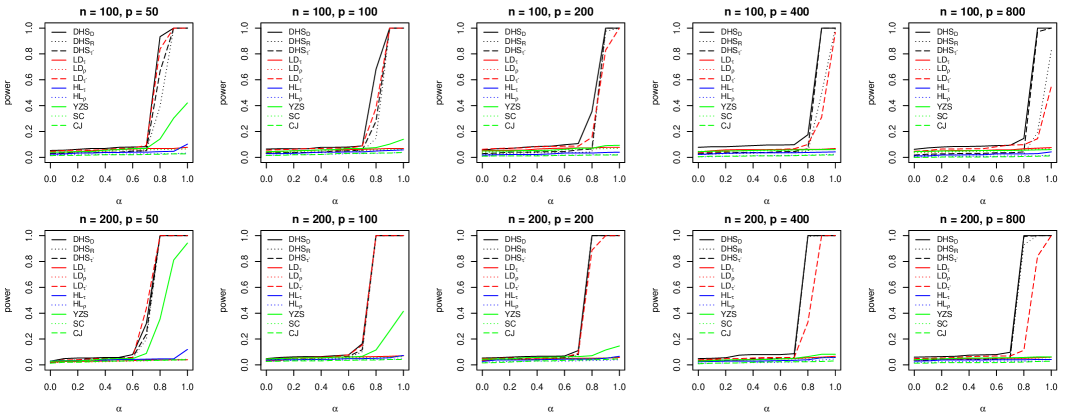
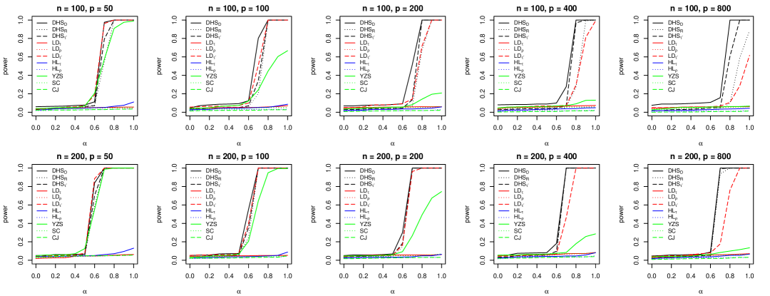
Figure 2: Empirical powers of the eleven competing tests in continued Example 5.2(a) (first two rows) and continued Example 5.2(b) (last two rows). The y-axis represents the power based on 5,000 replicates and the x-axis represents the level of a desired signal.

 

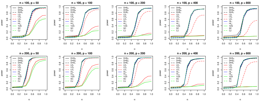
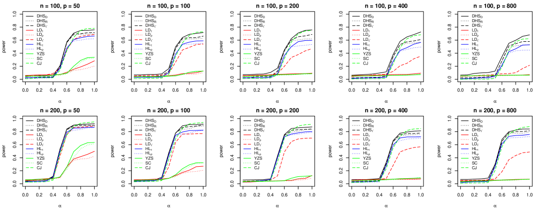
Figure 3: Empirical powers of the eleven competing tests in continued Example 5.3(a) (first two rows) and continued Example 5.3(b) (last two rows). The y-axis represents the power based on 5,000 replicates and the x-axis represents the level of a desired signal.

 

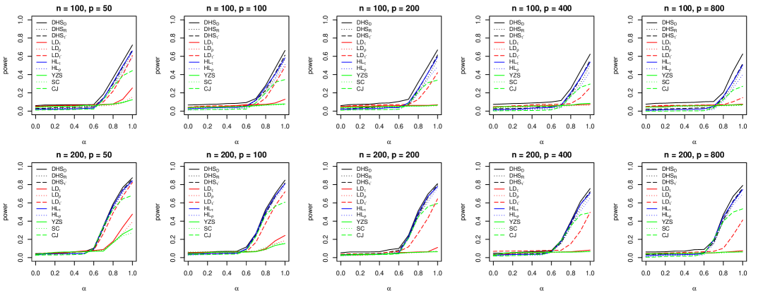
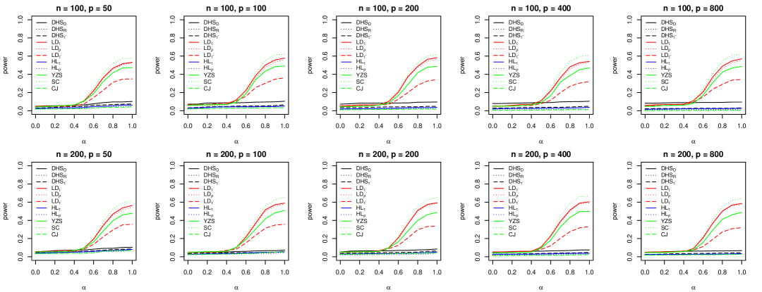
Figure 4: Empirical powers of the eleven competing tests in continued Example 5.3(c) (first two rows) and continued Example 5.4(a) (last two rows). The y-axis represents the power based on 5,000 replicates and the x-axis represents the level of a desired signal.

 

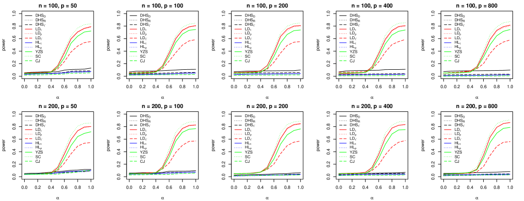
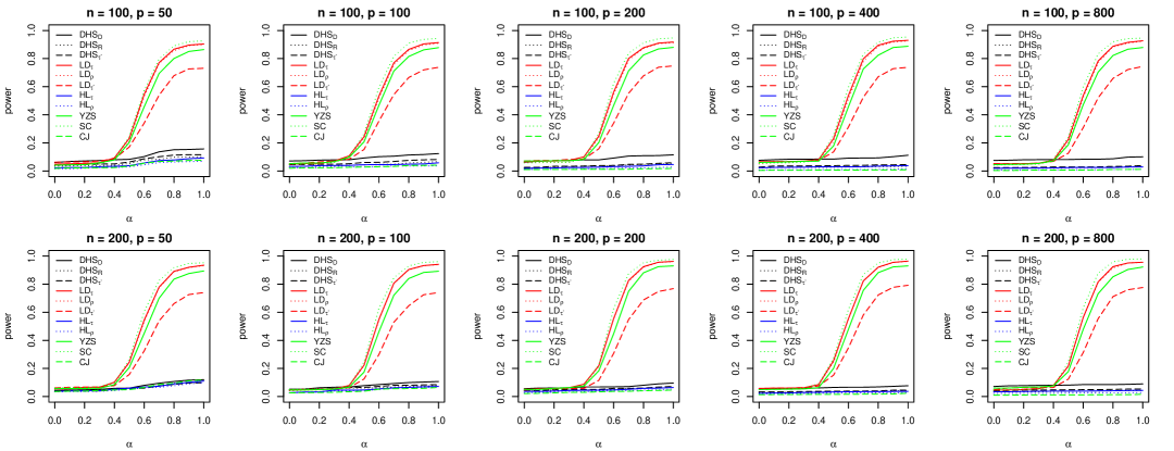
Figure 5: Empirical powers of the eleven competing tests in continued Example 5.4(b) (first two rows) and continued Example 5.4(c) (last two rows). The y-axis represents the power based on 5,000 replicates and the x-axis represents the level of a desired signal.

References

- Anderson, (2003) Anderson, T. W. (2003). An introduction to multivariate statistical analysis (3rd ed.). Wiley Series in Probability and Statistics. John Wiley and Sons, Inc., Hoboken, NJ.
- Arcones and Giné, (1993) Arcones, M. A. and Giné, E. (1993). Limit theorems for -processes. Ann. Probab., 21(3):1494–1542.
- Arratia et al., (1989) Arratia, R., Goldstein, L., and Gordon, L. (1989). Two moments suffice for Poisson approximations: the Chen-Stein method. Ann. Probab., 17(1):9–25.
- Bai et al., (2009) Bai, Z., Jiang, D., Yao, J.-F., and Zheng, S. (2009). Corrections to LRT on large-dimensional covariance matrix by RMT. Ann. Statist., 37(6B):3822–3840.
- Bao, (2019) Bao, Z. (2019). Tracy–Widom limit for Kendall’s tau. Ann. Statist., 47(6):3504–3532.
- Bao et al., (2012) Bao, Z., Pan, G., and Zhou, W. (2012). Tracy-Widom law for the extreme eigenvalues of sample correlation matrices. Electron. J. Probab., 17(88):1–32.
- Bentkus and Götze, (1997) Bentkus, V. and Götze, F. (1997). Uniform rates of convergence in the CLT for quadratic forms in multidimensional spaces. Probab. Theory Related Fields, 109(3):367–416.