Many-body theory of optical absorption in doped two-dimensional semiconductors

Abstract

In this article, we use a many-body approach to study the absorption spectra of electron-doped two-dimensional semiconductors. Optical absorption is modeled by a many-body scattering Hamiltonian which describes an exciton immersed in a Fermi sea. The interaction between electron and exciton is approximated by an effective scattering potential, and optical spectra are calculated by solving for the exciton Green’s function. From this approach, a trion state can be assigned as a bound state of an electron-exciton scattering process, and the doping-dependent phenomena observed in the spectra can be attributed to several many-body effects induced by the interaction with the Fermi sea. While the many-body scattering Hamiltonian can not solved exactly, we reduce the problem to two limiting solvable situations. The first approach approximates the full many-body problem by a simple scattering process between the electron and the exciton, with a self-energy obtained by solving a Bethe-Salpeter equation (BSE). An alternate approach assumes an infinite mass for the exciton, such that the many-body scattering Hamiltonian reduces to a Mahan-Noziéres-De Dominicis (MND) model. The exciton Green’s function can then be solved numerically exactly by a determinantal formulation, and the optical spectra show signatures of the Fermi-edge singularity at high doping densities. The full doping dependence and temperature dependence of the exciton and trion lineshapes are simulated via these two approximate approaches, with the results compared to each other and to experimental expectations.

I Introduction

A trion is a three-particle bound state which is composed of two electrons and one hole or two holes and one electronkheng1993observation . It can also be viewed as a negatively or positively charged exciton, which is generated by optical absorption in doped semiconductors or nanostructures. In the absorption or photoluminescence spectra of such systems at low doping density, the trion peak is observed on the low energy side of the exciton peak. The energy difference between the trion and exciton peaks in the zero doping-density limit is called the trion binding energy (denoted as $\Delta_{\text{T}}$). For semiconducting quantum wells, this binding energy is a few meVkheng1993observation ; huard2000bound ; astakhov2000oscillator ; ciulin2000radiative . The trion binding energy rises to about 30 meV for monolayer transition metal dichalcogenides (TMDCs)mak2013tightly ; berkelbach2013theory ; yang2015robust ; berkelbach2017optical and about 100 meV for single-wall carbon nanotubesakizuki2014nonlinear ; hartleb2015evidence .

While the nature of trion state in the limit of vanishing doping density is well studied and well understood, the physical description of the ”trion transition” as a function of doping remains unclearcombescot2003trion ; combescot2005many . A trion transition is an optical process of trion creation by photon absorption or trion annihilation via emission of light. In this discussion we consider specifically the optical absorption of electron-doped materials. Assuming electron doping can be described by altering the Fermi level in the conduction band, one can use the Fermi energy (denoted as $\varepsilon_{\text{F}}$) to estimate the scale of the electron doping density. According to various experimental measurementskheng1993observation ; huard2000bound ; astakhov2000oscillator ; ciulin2000radiative ; mak2013tightly ; yang2015robust , the lineshapes and intensities of exciton and trion transitions are notably affected by the doping density. For example as $\varepsilon_{\text{F}}$ increases, the exciton peak diminishes and the trion peak amplifies. The exciton peak begins to be depleted as the Fermi energy exceeds the trion binding energy ($\varepsilon_{\text{F}}\geq\Delta_{\text{T}}$). The total area of the combination of the two peaks in the absorption spectrum is relatively insensitive to the doping density variation. This behavior is connected to a sum rule that conserves the total oscillator strength. In addition, the energy splitting between the exciton peak and trion peak grows with increasing doping density, and is roughly given by $E_{\text{split}}\simeq\Delta_{\text{T}}+\varepsilon_{\text{F}}$. Some experiments also show that the exciton linewidth increases proportionally to the Fermi energy, while the trion linewidth is relatively insensitive to itastakhov2000oscillator . Finally, in the high doping density regime, the trion and exciton lineshapes are susceptible to temperature, and may become strongly asymmetrichuard2000bound ; astakhov2000oscillator . This latter feature implies the possible existence of a Fermi-edge singularity, which has been shown to exist in doped two-dimensional semiconductorsruckenstein1987many ; hawrylak1991optical ; brown1996evolution . All of these doping-dependent phenomena suggest the importance of many-body effects on the trion transition.

Various theories have been proposed to study the trion transition and simulate the doping-dependent optical spectra in semiconductorscombescot2003trion ; stebe1998optical ; esser2000photoluminescence ; bronold2000absorption ; esser2001theory ; suris2001excitons ; ossau2012optical ; shiau2012trion ; baeten2015many ; efimkin2017many , but many questions remain. A common picture of the trion transition is that of an electron-hole-pair generated in the presence of a background doping electron, from which the bound trion state forms. The transition amplitude connecting the exciton, the background electron and the trion state can be calculated by Fermi’s golden rulecombescot2003trion ; stebe1998optical ; esser2000photoluminescence ; shiau2012trion . This method is useful in the extremely low doping-density limit ($\varepsilon_{\text{F}}\ll\Delta_{\text{T}}$), but it fails to explain doping-dependent phenomena for higher doping densities.

An improved approach proposed by Bronoldbronold2000absorption ; ossau2012optical suggests a dynamical theory to explain the oscillator-strength competition between the exciton and trion transitions. Accordingly, the photogenerated valence hole scatters and transfers momentum to excite a Fermi sea electron-hole pair in the conduction band. The excited electron interacts with the photogenerated electron-hole pair to form a bound trion state. Along with the hole in the Fermi sea, the trion transition is interpreted as a dynamical trion-hole generation process. Bronold employed an exciton Green’s function formalism to simulate the absorption lineshape, and included the dynamical trion-hole generation by means of diagrammatic self-energy corrections. Within this formalism, the doping-dependent optical spectrum can be simulated in low doping-density regime ($\varepsilon_{\text{F}}<\Delta_{\text{T}}$), and the sum rule and oscillator strength transfer can be elucidated well. In addition to this study, Esser et al. also proposed a similar dynamical theory based on the density-matrix approachesser2001theory . They applied their theory to the optical spectra of one-dimensional nanostructures and found a good correspondence with expectations from experimental work. However, a detailed discussion of the trion and exciton lineshapes with respect to different doping densities and temperatures in two dimensions has not been carried out within these theoretical frameworks.

Other theories exist which describe the dynamical process of trion-hole generation. One such theory is the T-matrix model proposed by Suris et al.suris2001excitons ; ossau2012optical . Based on this approach, the trion binding energy can be obtained by solving a two-particle Lippmann-Schwinger equation which describes electron-exciton scattering. By assuming that only s-wave scattering is important and parametrizing the T-matrix phenomenologically, the authors found reasonable doping-dependent lineshape variation without concern for the details of the scattering potential. Recently, Efimkin and MacDonald extended the T-matrix model to create a Fermi-polaron theory of trion transitionefimkin2017many . The Fermi-polaron picture is normally employed in the study of the quasi-particle properties of impurity atoms immersed in, and strongly coupled to, an ultracold Fermi gasklawunn2011fermi ; schmidt2012fermi ; parish2013highly ; massignan2014polarons . In the present context, the impurity atom is replaced by an exciton and the Fermi gas is represented by the electron gas, such that the quasi-particle is given the name ”exciton-polaron.” In this framework, the trion transition can be interpreted as the lower-energy attractive exciton-polaron branch. A derivable scattering model has been built by approximating the electron-exciton scattering potential by a contact interaction. The trion binding energy ($\Delta_{\text{T}}$) can then be calculated and the optical spectrum in full doping-density regime can also be obtained. However, the trion binding energy appears to be overestimated and is found to be dependent on an ultraviolet cut-off energy. Since the cut-off dependence is abruptly distinguishable with a trion model described by the three-particle Schrödinger-equation (presumably valid in the limit of vanishing doping density), the difference between the exciton-polaron state and the standard view of a trion state requires further investigation.

Based on concepts related to the Fermi-polaron approach, the Fermi-edge singularity associated with optical transitions in doped materials in the large exciton mass limit can also be studied. In particular, the Mahan-Noziéres-De Dominicis (MND) theory provides a framework to study the doping dependence of optical lineshapes in a dense electron gasmahan1967excitons ; ruckenstein1987many ; nozieres1969singularities ; gavoret1969optical ; combescot1971infrared ; mahan1980final ; von1982dynamical ; hawrylak1991optical ; mahan2013many ; pimenov2017fermi . Traditionally, the MND model is used to study an infinite-mass hole immersed in a Fermi sea in conjunction with an electron-hole scattering potential to explain the origin of edge singularity behavior. In a recent work, Baeten and Wouters applied an electron-exciton-scattering version of MND theory to the study of trion-polaritonsbaeten2015many . A long-range attractive Yukawa potential was used to simulate the electron-exciton interaction, and a trion transition can be obtained by numerically solving the model. The calculated doping-dependent optical spectra show some features coincident with behaviors observed in the optical spectra of TMDCs. However, the use of a Yukawa form of the scattering potential results in an overestimation of the trion binding energy and a doping-independent exciton linewidth. A better choice of model potential to describe electron-exciton scattering would be helpful to remedy these issues for applications in two-dimensional semiconductors.

The goal of the present work is to unify our understanding of the doping-dependent optical spectra of two-dimensional semiconductors via a systematic exploration of these related approaches. An appropriate electron-exciton scattering potential is derived, and a many-body scattering Hamiltonian which describes an exciton immersed in Fermi sea interacting with electrons through this potential is written down. While the many-body Hamiltonian can not be solved exactly, we reduce the description to two limiting situations which correspond to a particular type of electron-exciton scattering problem and the MND problem. The electron-exciton scattering problem can be solved by a Bethe-Salpeter equation (BSE), whose eigenspectrum can be included into the self-energy in a Green’s function formalism. We show that this approach, which we will call the BSE formalism in the following discussions, is conceptually equivalent to Bronold’s dynamical theory of trion-hole generation, Suris’ T-matrix model, and Efimkin-MacDonald’s Fermi-polaron theory. The doping-dependent exciton and trion lineshapes can be studied analytically in low doping-density regime, and extended to higher doping densities numerically. In the other limiting situation of infinite exciton mass the MND model is numerically solved and the optical spectrum is obtained by propagating the Green’s function in the time domain. The doping-dependent and temperature-dependent optical spectra of two-dimensional materials can then be numerically studied and compared to that of the BSE approach and to experimental expectations.

This article is organized as follows. In Sec. II, we give a heuristic review of the theories of optical transitions in doped semiconductors by writing down the wavefunctions associated with the optically-generated quasi-particles. The concepts and relationship between the exciton state, trion state, trion transition, electron-exciton scattering, dynamical trion-hole generation, Fermi-polaron and Fermi-edge singularity are introduced in a second-quantization language. Building on these concepts, the derivation of the electron-exciton scattering potential becomes manifest. In Sec. III, the electron-exciton scattering potential is derived and the many-body scattering Hamiltonian is written down. Approximate methods based on the BSE formalism and the MND theory to solve the Hamiltonian are introduced. The connection between the BSE formalism and Efimkin-MacDonald’s Fermi-polaron theory is also discussed. By using the self-energy from the BSE formalism, the exciton and trion transitions are analyzed in Sec. IV. Numerical calculations within both the BSE formalism and the MND theory are provided in Sec. V to study the exciton and trion lineshapes. The optical energy renormalization and Pauli-blocking effects due to electron-doping in two-dimensional materials are also discussed. Finally, our conclusions are given in Sec. VI.

II Heuristic wavefunction theory

In the case of weak light-matter interaction, the optical absorption of solid-state materials can be realized as a dynamical conduction process. The creation of an exciton is associated with the electron-hole-pair generation process, whereby the electron and hole become bound due to the attractive Coulomb interaction between them. The frequency-dependent transition spectral density of this process is proportional to

$$\mathcal{A}(\omega)\sim\frac{1}{\omega}|\braket{\text{X}_{\mathbf{K}}}{\hat{j}}{0}|^{2}\delta(\omega-\varepsilon_{\text{X},\mathbf{K}}),$$ (1)

where $\ket{\text{X}_{\mathbf{K}}}$ is an exciton state, $\ket{0}$ is the ground state, $\varepsilon_{\text{X},\mathbf{K}}=\braket{\text{X}_{\mathbf{K}}}{\hat{\mathcal{H}}}{\text{X}_{\mathbf{K}}}-\braket{0}{\hat{\mathcal{H}}}{0}$ is the exciton transition energy, and $\hat{j}$ is the current operatormahan2013many . The ground state can be described as one with the valence band fully occupied and the conduction band completely empty. The exciton state can then be written as $\ket{\text{X}_{\mathbf{K}}}=\hat{X}^{\dagger}_{\mathbf{K}}\ket{0}$, where

$$\hat{X}^{\dagger}_{\mathbf{K}} = \sum_{\mathbf{p}}\Psi_{\text{X},\mathbf{p}}\hat{c}^{\dagger}_{\mathbf{p}+\mathbf{K}}\hat{d}^{\dagger}_{-\mathbf{p}},$$ (2)

is the exciton creation operator, $\hat{c}^{\dagger}_{\mathbf{p}}$ is the creation operator of electron in the conduction band with quasi-momentum $\mathbf{p}$, $\hat{d}^{\dagger}_{\mathbf{p}}$ is the creation operator of hole in the valence band, and $\Psi_{\text{X},\mathbf{p}}$ is the exciton wavefunction. For a direct band-gap semiconductor, the electric current operator is written as

$$\hat{{j}}\simeq e\sum_{\mathbf{k}}\left(\mathcal{P}_{\mathbf{k}\text{cv}}\hat{c}^{\dagger}_{\mathbf{k}}\hat{d}^{\dagger}_{\mathbf{k}}+\mathcal{P}^{*}_{\mathbf{k}\text{cv}}\hat{d}_{\mathbf{k}}\hat{c}_{\mathbf{k}}\right),$$ (3)

where $\mathcal{P}_{\mathbf{k}\text{cv}}$ is the momentum matrix element. Therefore, a vertical transition selection rule $\braket{\text{X}_{\mathbf{0}}}{\hat{j}}{0}\neq{0}$ can be found.

On the other hand, the trion transition is more complex. The trion state can be written as $\ket{\text{T}_{\mathbf{Q}}}=\hat{T}^{\dagger}_{\mathbf{Q}}\ket{0}$, where the trion creation operator is

$$\hat{T}^{\dagger}_{\mathbf{Q}} = \sum_{\mathbf{p}\mathbf{q}}\Psi_{\text{T},\mathbf{p}\mathbf{q}}\hat{c}^{\dagger}_{\mathbf{p}+\frac{m_{\text{e}}}{M_{\text{T}}}\mathbf{Q}}\hat{c}^{\dagger}_{\mathbf{q}+\frac{m_{\text{e}}}{M_{\text{T}}}\mathbf{Q}}\hat{d}^{\dagger}_{-\mathbf{p}-\mathbf{q}+\frac{m_{\text{h}}}{M_{\text{T}}}\mathbf{Q}},$$ (4)

with $\Psi_{\text{T},\mathbf{p}\mathbf{q}}$ the trion wavefunction, $m_{\text{e}}$ the electron mass, $m_{\text{e}}$ the hole mass, and $M_{\text{T}}=2m_{\text{e}}+m_{\text{h}}$ the trion mass. With these assumptions, it is found that the transition amplitude $\braket{\text{T}_{\mathbf{Q}}}{\hat{j}}{0}$ is zero. A commonly used modification is to employ a different initial state in calculating the transition rate. Assuming that the initial state is $\ket{\text{e}_{\mathbf{Q}}}=\hat{c}^{\dagger}_{\mathbf{Q}}\ket{0}$, such that the transition amplitude $\braket{\text{T}_{\mathbf{Q}}}{\hat{j}}{\text{e}_{\mathbf{Q}}}$ is non-zero, then the transition spectral density based on Fermi’s golden rule isstebe1998optical ; esser2000photoluminescence ; shiau2012trion

$$\mathcal{A}(\omega) \sim \frac{1}{\omega}\left(1-\sigma\sum\nolimits_{\mathbf{Q}}n_{\mathbf{Q}}\right)|\braket{\text{X}_{\mathbf{0}}}{\hat{j}}{0}|^{2}\delta\left(\omega-\varepsilon_{\text{X}}\right)$$

$$+\frac{\sigma}{\omega}\sum_{\mathbf{Q}}n_{\mathbf{Q}}|\braket{\text{T}_{\mathbf{Q}}}{\hat{j}}{\text{e}_{\mathbf{Q}}}|^{2}\delta\left(\omega-\varepsilon_{\text{T},\mathbf{Q}}+\varepsilon_{\text{e},\mathbf{Q}}\right),$$

where $\sigma$ is an adjustable parameter related to the photon-electron scattering cross-section, $n_{\mathbf{Q}}$ is the electron density distribution of the $\ket{\text{e}_{\mathbf{Q}}}$ state, $\varepsilon_{\text{T},\mathbf{Q}}=\braket{\text{T}_{\mathbf{Q}}}{\hat{\mathcal{H}}}{\text{T}_{\mathbf{Q}}}-\braket{0}{\hat{\mathcal{H}}}{0}$ is the trion transition energy, and $\varepsilon_{\text{e},\mathbf{Q}}=\braket{\text{e}_{\mathbf{Q}}}{\hat{\mathcal{H}}}{\text{e}_{\mathbf{Q}}}-\braket{0}{\hat{\mathcal{H}}}{0}$ is the electron quasi-particle energy. Although this is an ad hoc description, the above formula is quite useful and physical in the extreme low doping-density limit ($\varepsilon_{\text{F}}\ll\Delta_{\text{T}}$). Particularly if we assume $\braket{\text{X}_{\mathbf{0}}}{\hat{j}}{0}\simeq\braket{\text{T}_{\mathbf{Q}}}{\hat{j}}{\text{e}_{\mathbf{Q}}}$, integration over the rate constant $\int\text{d}\omega\;\mathcal{A}(\omega)$ is roughly invariant to doping density, implying that the lowest-order sum rule is fulfilled. However, with higher doping density and thus $\sum_{\mathbf{Q}}n_{\mathbf{Q}}\gtrsim 1/\sigma$, the transition rate constant becomes negative and the formula becomes unphysical.

Another description of the trion transition is given by Fermi-polaron approachefimkin2017many . Based on this framework, the ground state is described by the Fermi sea formed by the electron gas that resides in the conduction band, in addition to the fully occupied valence band. When an exciton is excited, the Coulomb interaction between the exciton and the Fermi sea induces electron-hole polarization near the Fermi surface. The Fermi-polaron state $\ket{\text{P}}$ can be written asparish2013highly

$$\ket{\text{P}} = \Phi_{0}\hat{X}^{\dagger}_{\mathbf{0}}\ket{\text{FS}}+\sum_{\mathbf{q},\mathbf{K}}\Phi_{\mathbf{K}}\hat{X}^{\dagger}_{-\mathbf{K}}\hat{c}^{\dagger}_{\mathbf{q}+\mathbf{K}}\hat{c}_{\mathbf{q}}\ket{\text{FS}},$$ (6)

where $\Phi_{0}$, $\Phi_{\mathbf{K}}$ are superposition coefficients, and $\ket{\text{FS}}$ is the Fermi sea conduction-band plus fully occupied valence-band state. The coefficients $\Phi_{0}$, $\Phi_{\mathbf{K}}$ can be evaluated by treating $\ket{\text{P}}$ as variational wavefunction to minimize the variational energy. Since we are not considering the Coulomb interaction among the electrons in the Fermi sea, we can assume the Fermi sea is composed of independent electrons and then replace $\ket{\text{FS}}$ by $\hat{c}^{\dagger}_{\mathbf{Q}}\ket{\tilde{\text{FS}}}$, where $\ket{\tilde{\text{FS}}}=\hat{c}_{\mathbf{Q}}\ket{\text{FS}}$. Therefore, the Fermi-polaron state becomes

$$\ket{\text{P}} = \Phi_{0}\hat{X}^{\dagger}_{\mathbf{0}}c^{\dagger}_{\mathbf{Q}}\ket{\tilde{\text{FS}}}+\sum_{\mathbf{K}}\Phi_{\mathbf{K}}\hat{X}^{\dagger}_{-\mathbf{K}}\hat{c}^{\dagger}_{\mathbf{Q}+\mathbf{K}}\ket{\tilde{\text{FS}}}.$$ (7)

If we define the incoming state and outgoing state as

$$\ket{\text{in}}=\hat{X}^{\dagger}_{\mathbf{0}}c^{\dagger}_{\mathbf{Q}}\ket{\tilde{\text{FS}}},\hskip 8.61108pt\ket{\text{out}}=\hat{X}^{\dagger}_{-\mathbf{K}}\hat{c}^{\dagger}_{\mathbf{Q}+\mathbf{K}}\ket{\tilde{\text{FS}}},$$ (8)

then solving for the variational coefficients reduces to an electron-exciton scattering problem. If there is an attractive interaction between the electron and the exciton, an extra bound state may exist, which can be interpreted as the trion state.

Although the Fermi-polaron state and the trion state appear to be different, the two pictures can be connected if the electron-exciton bound state can be related to the trion state by a linear transformation with the coefficient $\Phi_{\mathbf{K}}$,

$$\hat{T}^{\dagger}_{\mathbf{Q}} = \sum_{\mathbf{K}}\Phi_{\mathbf{K}}\hat{X}^{\dagger}_{-\mathbf{K}}\hat{c}^{\dagger}_{\mathbf{Q}+\mathbf{K}}.$$ (9)

In this case, the Fermi-polaron state can be rewritten as

$$\ket{\text{P}} = \Phi_{\mathbf{0}}\hat{X}^{\dagger}_{\mathbf{0}}\ket{\text{FS}}+\sum_{\mathbf{Q}}\hat{T}^{\dagger}_{\mathbf{Q}}\hat{c}_{\mathbf{Q}}\ket{\text{FS}}.$$ (10)

Therefore, Fermi-polaron generation can be seen as the collective excitation of trion-hole-pair states near the Fermi surface, where the hole is created by annihilating an electron in the Fermi sea. If the trion-hole interaction energy is small in compared to the trion binding energy, the excitation will show particle-like features, such that the process can be interpreted as trion generation. The collective nature of dynamical trion-hole generation and the trion-hole interaction will however affect the trion and exciton transition energies and lineshapes.

The problem of the Fermi-edge singularity is naturally connected to that of the Fermi-polaron, since they both describe an impurity immersed in, and interacting with, the Fermi sea. In the case under consideration here, the impurity is an exciton. While the scattering function formalism describes single electron-hole pair excitation near Fermi surface, the Fermi-edge singularity is an effect caused by multiple electron-hole pair excitation. Based on the Fermi-polaron state wavefunction, if the exciton mass is much larger than the electron mass and the electron-density is sufficiently high, the edge singularity state will include the multiple-excitation terms as

$$\ket{\text{ES}} = \Phi_{0}\hat{X}^{\dagger}_{\mathbf{0}}\ket{\text{FS}}+\sum_{\mathbf{K}}\Phi_{\mathbf{K}}\hat{X}^{\dagger}_{-\mathbf{K}}\hat{B}^{\dagger}_{\mathbf{K}}\ket{\text{FS}}$$ (11)

$$+\sum_{\mathbf{K}_{1}\mathbf{K}_{2}}\Phi_{\mathbf{K}_{1},\mathbf{K}_{2}}\hat{X}^{\dagger}_{-\mathbf{K}_{1}-\mathbf{K}_{2}}\left(\hat{B}^{\dagger}_{\mathbf{K}_{1}}\hat{B}^{\dagger}_{\mathbf{K}_{2}}\right)\ket{\text{FS}}+\cdots$$

$$+\sum_{\mathbf{K}_{1}\cdots\mathbf{K}_{n}}\Phi_{\mathbf{K}_{1}\cdots\mathbf{K}_{n}}\hat{X}^{\dagger}_{-\sum^{n}_{\alpha=1}\mathbf{K}_{\alpha}}\left(\prod^{n}_{\alpha^{\prime}=1}\hat{B}^{\dagger}_{\mathbf{K}_{\alpha^{\prime}}}\right)\ket{\text{FS}}$$

$$+\cdots,$$

where $\hat{B}^{\dagger}_{\mathbf{K}}=\sum_{\mathbf{q}}\hat{c}^{\dagger}_{\mathbf{q}+\mathbf{K}}\hat{c}_{\mathbf{q}}$ is the Fermi sea electron-hole excitation operator. If the hole and electron are excited within the energy scale of the Fermi surface, the Fermi sea electron-hole excitation energy will be close to zero. When the exciton mass is large, the exciton kinetic energy makes a vanishingly small contribution to the excitation energy. Therefore, the all multiple-excitation terms can have an excitation energy coincident with the exciton transition energy, producing a divergence in the oscillator strength close to the exciton transition energy.

To describe all relevant transitions, the Fermi-polaron state wavefunction in Eq. (6) or the edge-singularity state wavefunction in Eq. (11) can act as variational wavefunctions, and the wavefunction coefficients can be treated as variational parameters. If the lowest-energy solution of the variation problem has a lower energy than the exciton transition energy, the state may be interpreted as a trion bound state. Other solutions with energies higher than the exciton transition energy can be interpreted as electron-exciton scattering states. However, the variational problem is too difficult to solve in the electron-hole basis due to the large number of degrees of freedom. Approximations are needed in order to reduce the numerical effort. In the present work, one approximation we consider is to reduce the electron-hole basis to an electron-exciton basis. The exciton state is presumed to be a particle state that can not be decomposed, and the exciton transition energy is parametrized. Via this approximation, the number of degrees of freedom is greatly reduced. In Sec. III, we will give the formal theory of this reduction and provide the methods of solution.

III Formal theory

In this section, we give a formal theory of a trion transition based on a many-body scattering Hamiltonian, which includes electron and exciton kinetic energies and an appropriate electron-exciton scattering potential. We assume that, by solving the exciton Green’s function of the many-body scattering Hamiltonian, the trion transition can be found and the doping dependence of the lineshapes can be explained. In Sec. III.1 and Sec. III.2 the electron-exciton scattering potential is derived and the many-body scattering Hamiltonian is introduced. However the many-body Hamiltonian is not exactly solvable, and some approximations must be employed. One avenue to approximation is the reduction of the many-body problem to a two-particle scattering problem between an electron and an exciton, with the inclusion of the scattering processes directly into the exciton self-energy. In Sec. III.3, we introduce this method and show that it is essentially equivalent to Efimkin and MacDonald’s Fermi-polaron theory for optical absorption of a two-dimensional doped semiconductorefimkin2017many . While their Fermi-polaron theory requires a cut-off energy-dependent trion binding energy, an alternate method is preferred. In Sec. III.4, a BSE formalism that employs Bronold’s dynamical theory of trion-hole generationbronold2000absorption is derived. Finally, we consider another approximate method valid in the limiting situation where the exciton mass is infinitely large. Here, the many-body scattering Hamiltonian is reduced to an electron-exciton version of the MND modelbaeten2015many . In Sec. III.5, the MND model and its numerical method of solution are introduced.

III.1 Scattering potential

In order to find the scattering potential between electron and exciton, we consider the electron-hole Hamiltonian for electron-doped semiconductorshaug2009quantum

$$\hat{\mathcal{H}} = \sum_{\mathbf{k}}\left(\varepsilon_{\text{e},\mathbf{k}}\hat{c}^{\dagger}_{\mathbf{k}}\hat{c}_{\mathbf{k}}+\varepsilon_{\text{h},\mathbf{k}}\hat{d}^{\dagger}_{\mathbf{k}}\hat{d}_{\mathbf{k}}\right)$$

$$+\sum_{\mathbf{k}\mathbf{k}^{\prime}\mathbf{q}}\frac{U_{\mathbf{q}}}{2}\Big{(}\hat{c}^{\dagger}_{\mathbf{k}+\mathbf{q}}\hat{c}^{\dagger}_{\mathbf{k}^{\prime}-\mathbf{q}}\hat{c}_{\mathbf{k}^{\prime}}\hat{c}_{\mathbf{k}}-2\hat{c}^{\dagger}_{\mathbf{k}+\mathbf{q}}\hat{d}^{\dagger}_{-\mathbf{k}^{\prime}-\mathbf{q}}\hat{d}_{-\mathbf{k}^{\prime}}\hat{c}_{\mathbf{k}}\Big{)},$$

where the Hamiltonian contains kinetic energy terms and Coulomb interaction terms, $\varepsilon_{\text{e},\mathbf{k}}$, $\varepsilon_{\text{h},\mathbf{k}}$ are the kinetic energies of electron and hole, and $U_{\mathbf{q}}=v_{\mathbf{q}}/{L^{\text{D}}}$, with $v_{\mathbf{q}}$ the Coulomb potential and $L^{\text{D}}$ the dimension of the system. The scattering transition amplitudes can be calculated by using the electron-exciton basis states of Eq. (8). Note that the $\mathbf{Q}$ of all basis states are equal in order to fulfill momentum conservation. For the diagonal term of the Hamiltonian matrix, we find

$$\left(\bra{\tilde{\text{FS}}}\hat{c}_{\mathbf{Q}+\mathbf{K}}\hat{X}_{-\mathbf{K}}\right)\hat{\mathcal{H}}\left(\hat{X}^{\dagger}_{-\mathbf{K}}\hat{c}^{\dagger}_{\mathbf{Q}+\mathbf{K}}\ket{\tilde{\text{FS}}}\right)$$ (13)

$$\simeq E_{\tilde{\text{FS}}}+\varepsilon_{\text{X},-\mathbf{K}}+\varepsilon_{\text{e},\mathbf{Q}+\mathbf{K}},$$

where $E_{\tilde{\text{FS}}}=\bra{\tilde{\text{FS}}}\hat{\mathcal{H}}\ket{\tilde{\text{FS}}}=\bra{\text{FS}}\hat{\mathcal{H}}\ket{\text{FS}}-\varepsilon_{\text{e},\mathbf{Q}}$ is the Fermi sea ground state energy and $\varepsilon_{\text{X},\mathbf{K}}$ is the exciton excitation energy. The nondiagonal terms of the Hamiltonian matrix give the scattering potential

$$V_{\mathbf{K}\mathbf{K}^{\prime},\mathbf{Q}} = \left(\bra{\tilde{\text{FS}}}\hat{c}_{\mathbf{Q}+\mathbf{K}}\hat{X}_{-\mathbf{K}}\right)\hat{\mathcal{H}}\left(\hat{X}^{\dagger}_{-\mathbf{K}^{\prime}}\hat{c}^{\dagger}_{\mathbf{Q}+\mathbf{K}^{\prime}}\ket{\tilde{\text{FS}}}\right).$$

The exciton creation operator is assumed to be $\hat{X}^{\dagger}_{-\mathbf{K}}=\sum_{\mathbf{p}}\Psi_{\mathbf{p}}\hat{c}^{\dagger}_{\mathbf{p}}\hat{d}^{\dagger}_{-\mathbf{p}-\mathbf{K}}$, where $\Psi_{\mathbf{p}}$ is the exciton wavefunction. Since the electron-exciton interaction only involves the electron and hole degrees of freedom contained in the basis states, Eq. (LABEL:scattering) becomes

$$V_{\mathbf{K}\mathbf{K}^{\prime},\mathbf{Q}} = \sum_{\mathbf{p}\mathbf{p}^{\prime}}\Psi^{*}_{\mathbf{p}}\Psi_{\mathbf{p}^{\prime}}$$

$$\times\braket{\hat{c}_{\mathbf{Q}+\mathbf{K}}\hat{c}_{\mathbf{p}}\hat{d}_{-\mathbf{p}-\mathbf{K}}:\hat{\mathcal{H}}:\hat{c}^{\dagger}_{\mathbf{p}^{\prime}}\hat{d}^{\dagger}_{-\mathbf{p}^{\prime}-\mathbf{K}^{\prime}}\hat{c}^{\dagger}_{\mathbf{Q}+\mathbf{K}^{\prime}}},$$

where $:\hat{\mathcal{H}}:$ indicates that the number operators in the Hamiltonian are already contracted, i.e., $\braket{:\hat{d}^{\dagger}\hat{d}:}=\braket{:\hat{c}^{\dagger}\hat{c}:}=0$. The electron-electron interaction may be expressed

$$\braket{\hat{c}_{\mathbf{Q}+\mathbf{K}}\hat{d}_{-\mathbf{p}-\mathbf{K}}\hat{c}_{\mathbf{p}}:\hat{\mathcal{H}}_{\text{e-e}}:\hat{c}^{\dagger}_{\mathbf{p}^{\prime}}\hat{d}^{\dagger}_{-\mathbf{p}^{\prime}-\mathbf{K}^{\prime}}\hat{c}^{\dagger}_{\mathbf{Q}+\mathbf{K}^{\prime}}} = \sum_{\mathbf{k}\mathbf{k}^{\prime}\mathbf{q}}\frac{U_{\mathbf{q}}}{2}\braket{\hat{c}_{\mathbf{Q}+\mathbf{K}}\hat{d}_{-\mathbf{p}-\mathbf{K}}\hat{c}_{\mathbf{p}}:\hat{c}^{\dagger}_{\mathbf{k}+\mathbf{q}}\hat{c}^{\dagger}_{\mathbf{k}^{\prime}-\mathbf{q}}\hat{c}_{\mathbf{k}^{\prime}}\hat{c}_{\mathbf{k}}:\hat{c}^{\dagger}_{\mathbf{p}^{\prime}}\hat{d}^{\dagger}_{-\mathbf{p}^{\prime}-\mathbf{K}^{\prime}}\hat{c}^{\dagger}_{\mathbf{Q}+\mathbf{K}^{\prime}}}$$ (16)

$$= \delta_{\mathbf{p}-\mathbf{p}^{\prime},\mathbf{K}^{\prime}-\mathbf{K}}\big{(}U_{\mathbf{K}^{\prime}-\mathbf{K}}-U_{\mathbf{p}-\mathbf{Q}-\mathbf{K}^{\prime}}\big{)}.$$

$$\braket{\hat{c}_{\mathbf{Q}+\mathbf{K}}\hat{d}_{-\mathbf{p}-\mathbf{K}}\hat{c}_{\mathbf{p}}:\hat{\mathcal{H}}_{\text{e-h}}:\hat{c}^{\dagger}_{\mathbf{p}^{\prime}}\hat{d}^{\dagger}_{-\mathbf{p}^{\prime}-\mathbf{K}^{\prime}}\hat{c}^{\dagger}_{\mathbf{Q}+\mathbf{K}^{\prime}}} = -\sum_{\mathbf{k}\mathbf{k}^{\prime}\mathbf{q}}U_{\mathbf{q}}\braket{\hat{c}_{\mathbf{Q}+\mathbf{K}}\hat{d}_{-\mathbf{p}-\mathbf{K}}\hat{c}_{\mathbf{p}}:\hat{c}^{\dagger}_{\mathbf{k}+\mathbf{q}}\hat{d}^{\dagger}_{-\mathbf{k}^{\prime}-\mathbf{q}}\hat{d}_{-\mathbf{k}^{\prime}}\hat{c}_{\mathbf{k}}:\hat{c}^{\dagger}_{\mathbf{p}^{\prime}}\hat{d}^{\dagger}_{-\mathbf{p}^{\prime}-\mathbf{K}^{\prime}}\hat{c}^{\dagger}_{\mathbf{Q}+\mathbf{K}^{\prime}}}$$

$$= -\big{(}U_{\mathbf{p}-\mathbf{p}^{\prime}}-U_{\mathbf{Q}+\mathbf{K}-\mathbf{p}^{\prime}}\delta_{\mathbf{p},\mathbf{Q}+\mathbf{K}^{\prime}}-U_{\mathbf{p}-\mathbf{Q}-\mathbf{K}^{\prime}}\delta_{\mathbf{Q}+\mathbf{K},\mathbf{p}^{\prime}}+U_{\mathbf{K}-\mathbf{K}^{\prime}}\delta_{\mathbf{p},\mathbf{p}^{\prime}}\big{)}.$$

The scattering potential can thus be written as

$$V_{\mathbf{K}\mathbf{K}^{\prime},\mathbf{Q}} = V^{\text{di-ee}}_{\mathbf{K}\mathbf{K}^{\prime}}+V^{\text{ex-ee}}_{\mathbf{K}\mathbf{K}^{\prime},\mathbf{Q}}+V^{\text{di-eh}}_{\mathbf{K}\mathbf{K}^{\prime}}+V^{\text{ex-eh}}_{\mathbf{K}\mathbf{K}^{\prime},\mathbf{Q}},$$ (18)

with a direct electron-electron interaction $V^{\text{di-ee}}_{\mathbf{K}\mathbf{K}^{\prime}}$, an exchange electron-electron interaction $V^{\text{ex-ee}}_{\mathbf{K}\mathbf{K}^{\prime},\mathbf{Q}}$, a direct electron-hole interaction $V^{\text{di-eh}}_{\mathbf{K}\mathbf{K}^{\prime}}$, and an exchange electron-hole interaction $V^{\text{ex-eh}}_{\mathbf{K}\mathbf{K}^{\prime},\mathbf{Q}}$. The interactions are

$$V^{\text{di-ee}}_{\mathbf{K}\mathbf{K}^{\prime}} = \sum_{\mathbf{p}}U^{*}_{\mathbf{K}-\mathbf{K}^{\prime}}\Psi^{*}_{\mathbf{p}}\Psi_{\mathbf{p}+\mathbf{K}-\mathbf{K}^{\prime}},$$ (19)

$$V^{\text{ex-ee}}_{\mathbf{K}\mathbf{K}^{\prime},\mathbf{Q}} = -\sum_{\mathbf{p}}U_{\mathbf{p}}\Psi^{*}_{\mathbf{p}+\mathbf{Q}+\mathbf{K}^{\prime}}\Psi_{\mathbf{p}+\mathbf{Q}+\mathbf{K}},$$ (20)

$$V^{\text{di-eh}}_{\mathbf{K}\mathbf{K}^{\prime}} = -U_{\mathbf{K}-\mathbf{K}^{\prime}},$$ (21)

$$V^{\text{ex-eh}}_{\mathbf{K}\mathbf{K}^{\prime},\mathbf{Q}} = \sum_{\mathbf{p}}\big{(}U^{*}_{\mathbf{p}}\Psi^{*}_{\mathbf{Q}+\mathbf{K}^{\prime}}\Psi_{\mathbf{p}+\mathbf{Q}+\mathbf{K}}$$ (22)

$$+U_{\mathbf{p}}\Psi^{*}_{\mathbf{p}+\mathbf{Q}+\mathbf{K}^{\prime}}\Psi_{\mathbf{Q}+\mathbf{K}}\big{)}.$$

It it important to note that the present derivation does not consider the spin degree of freedom. Therefore the electron and hole creation operators contained in the trion creation operator can be seen to have the same spin quantum number. In this case, the exchange interaction is of opposite sign to that of the direct interaction. However, if the two electrons which comprise the electron portion of the trion have different spin quantum numbers, the exchange interaction can be zero or of the same sign as the direct interaction, and will depend on the overall spin state of the trion. The spin dependence of the trion transition is beyond the scope of this work, and we will ignore all exchange interactions in the following discussion. The effect of spin and exchange interactions will be studied in future work.

Assuming $U_{\mathbf{q}}=U^{*}_{\mathbf{q}}$ and $\Delta\mathbf{K}=\mathbf{K}-\mathbf{K}^{\prime}$, the total direct interaction can be written as

$$V^{\text{di}}_{\mathbf{K}\mathbf{K}^{\prime}} = -U_{\Delta\mathbf{K}}\left(1-\sum_{\mathbf{p}}\Psi^{*}_{\mathbf{p}}\Psi_{\mathbf{p}+\Delta\mathbf{K}}\right).$$ (23)

The wavefunction overlap $\sum_{\mathbf{p}}\Psi^{*}_{\mathbf{p}}\Psi_{\mathbf{p}+\Delta\mathbf{K}}$ is unity for $\Delta\mathbf{K}=0$ and tends to zero as $\Delta\mathbf{K}\rightarrow\infty$. Via Taylor expansion with respect to $|\Delta\mathbf{K}|$, the wavefunction overlap can be expressed as

$$\sum_{\mathbf{p}}\Psi^{*}_{\mathbf{p}}\Psi_{\mathbf{p}+\Delta\mathbf{K}} \simeq \sum_{\mathbf{p}}\Psi^{*}_{\mathbf{p}}\Psi_{\mathbf{p}}-\mathtt{i}|\Delta\mathbf{K}|\sum_{\mathbf{p}}\Psi^{*}_{\mathbf{p}}\left(\mathtt{i}\frac{\partial}{\partial{p}}\right)\Psi_{\mathbf{p}}$$

$$-\frac{1}{2}|\Delta\mathbf{K}|^{2}\sum_{\mathbf{p}}\Psi^{*}_{\mathbf{p}}\left(\mathtt{i}\frac{\partial}{\partial{p}}\right)^{2}\Psi_{\mathbf{p}}+\cdots.$$

Assuming the exciton wavefunction is given by the nodeless 1s-orbital wavefunction obtained from the two-dimensional hydrogen atom problem, the wavefunction overlap can be approximated as

$$\sum_{\mathbf{p}}\Psi^{*}_{\mathbf{p}}\Psi_{\mathbf{p}+\Delta\mathbf{K}} \simeq \exp\left(-\frac{1}{2}|\Delta\mathbf{K}|^{2}\xi^{2}\right),$$ (25)

where $\xi^{2}=\sum_{\mathbf{p}}\Psi^{*}_{\mathbf{p}}\left(\mathtt{i}{\partial}/{\partial{p}}\right)^{2}\Psi_{\mathbf{p}}$, since it can be shown that $\sum_{\mathbf{p}}\Psi^{*}_{\mathbf{p}}\left(\mathtt{i}{\partial}/{\partial{p}}\right)\Psi_{\mathbf{p}}=0$ for a 1s-orbital. The exponential form of the approximate wavefunction overlap reproduces the correct behavior as $\Delta\mathbf{K}\rightarrow{0}$. The characteristic length $\xi$ can be rewritten as

$$\xi^{2} = \int\text{d}^{\text{D}}\mathbf{r}\;\tilde{\Psi}^{*}(\mathbf{r})|\mathbf{r}|^{2}\tilde{\Psi}(\mathbf{r}),$$ (26)

where $\tilde{\Psi}(\mathbf{r})$ is the real space Fourier transform of $\Psi_{\mathbf{p}}$. Therefore, $\xi$ can be interpreted as the root-mean-square exciton radius.

III.2 Many-body scattering Hamiltonian

With exchange interactions ignored, the many-body scattering Hamiltonian for an exciton immersed in an electron gas can be written as

$$\hat{\mathcal{H}}_{\text{eff}} = \sum_{\mathbf{K}}\varepsilon_{\text{X},\mathbf{K}}\hat{X}^{\dagger}_{\mathbf{K}}\hat{X}_{\mathbf{K}}+\sum_{\mathbf{k}}\varepsilon_{\text{e},\mathbf{k}}\hat{c}^{\dagger}_{\mathbf{k}}\hat{c}_{\mathbf{k}}$$ (27)

$$+\sum_{\mathbf{Q}\mathbf{K}\mathbf{K}^{\prime}}V_{\mathbf{K},\mathbf{K}^{\prime}}\hat{c}^{\dagger}_{\mathbf{K}+\mathbf{Q}}\hat{c}_{\mathbf{K}^{\prime}+\mathbf{Q}}\hat{X}^{\dagger}_{-\mathbf{K}}\hat{X}_{-\mathbf{K}^{\prime}},$$

where the exciton kinetic energy and electron kinetic energy can be written as

$$\varepsilon_{\text{X},\mathbf{K}}=\varepsilon_{\text{X}}+\frac{|\mathbf{K}|^{2}}{2M_{\text{X}}},\hskip 8.61108pt\varepsilon_{\text{e},\mathbf{k}}=\frac{|\mathbf{k}|^{2}}{2m_{\text{e}}},$$ (28)

where $\varepsilon_{\text{X}}=\varepsilon_{\text{X},\mathbf{K}=\mathbf{0}}$ is the exciton transition energy, $M_{\text{X}}$ is the exciton mass and $m_{\text{e}}$ is the electron mass. The scattering potential is assumed to have the form

$$V_{\mathbf{K},\mathbf{K}^{\prime}} = -\frac{v_{\mathbf{K}-\mathbf{K}^{\prime}}}{L^{2}}\left[1-\exp\left(-\frac{1}{2}|\mathbf{K}-\mathbf{K}^{\prime}|^{2}\xi^{2}\right)\right],$$ (29)

where $v_{\mathbf{K}-\mathbf{K}^{\prime}}$ can be taken to be the screened Coulomb potential and $\xi$ is the exciton radius.

The electric current operator for the electron-hole excitation process is given by

$$\hat{{j}} \simeq e\left(\mathcal{P}\hat{X}^{\dagger}_{\mathbf{0}}+\mathcal{P}^{*}\hat{X}_{\mathbf{0}}\right),$$ (30)

where $\mathcal{P}=\sum_{\mathbf{p}}\Psi_{\mathbf{p}}\mathcal{P}_{\mathbf{p}\text{cv}}$ is the transition momentum matrix element. The absorption spectrum can be calculated by the real part of the optical conductivity or the imaginary part of the current-current response functionmahan2013many ,

$$\mathcal{A}(\omega) = 2\;\text{Re }\sigma(\omega)=-\frac{2}{\omega}\text{Im }\int^{\infty}_{-\infty}\text{d}t\;e^{\mathtt{i}\omega t}\pi^{\text{R}}(t),$$ (31)

$$\pi^{\text{R}}(t) = -\mathtt{i}\theta(t)\braket{\text{G}}{\left[\hat{j}(t),\hat{j}\right]}{\text{G}},$$ (32)

where $\theta(t)$ is a step function. The ground state $\ket{\text{G}}=\ket{0}\ket{\text{FS}}$ is a direct product of the vacuum state of the exciton ($\ket{0}$) and the Fermi sea of electrons ($\ket{\text{FS}}$). The response function can be obtained from the exciton Green’s function,

$$\pi^{\text{R}}(t) = e^{2}|\mathcal{P}|^{2}\mathcal{G}^{\text{R}}(t),$$ (33)

$$\mathcal{G}^{\text{R}}(t) = -\mathtt{i}\theta(t)\braket{\text{G}}{\left[\hat{X}_{\mathbf{0}}(t),\;\hat{X}^{\dagger}_{\mathbf{0}}\right]}{\text{G}}.$$ (34)

Then the absorption spectrum is expressed as

$$\mathcal{A}(\omega) = -\frac{2e^{2}}{\omega}|\mathcal{P}|^{2}\text{Im }\mathcal{G}^{\text{R}}(\omega).$$ (35)

The commutator in the Green’s function written in Eq. (34) implies that the exciton operators are presumed to be bosonic particles. However, since the ground state is an empty state for the exciton, and only single exciton generation is considered, the type of the commutation relation chosen in Eq. (34) does not alter the final results.

III.3 Scattering function and Fermi polaron theory

In the frequency domain, the exciton Green’s function can be solved by the Dyson’s equation

$$\mathcal{G}^{\text{R}}(\omega) = \frac{1}{\omega-\varepsilon_{\text{X}}-\Sigma^{\text{R}}(\omega)},$$ (36)

where $\Sigma^{\text{R}}(\omega)$ is the exciton self-energy. Based on perturbation theory, the lowest-order expression for the exciton self-energy is given by

$${\Sigma}^{\text{R}}(\omega) = \sum_{\mathbf{p}\mathbf{Q}}\frac{\left(1-n_{\mathbf{p}+\frac{m_{\text{e}}}{M_{\text{T}}}\mathbf{Q}}\right)n_{\mathbf{Q}}|V_{\mathbf{p}+\frac{m_{\text{e}}}{M_{\text{T}}}\mathbf{Q},\mathbf{Q}}|^{2}}{\omega-{\varepsilon}_{\text{X},-\mathbf{p}+\frac{M_{\text{X}}}{M_{\text{T}}}\mathbf{Q}}-{\varepsilon}_{\text{e},\mathbf{p}+\frac{m_{\text{e}}}{M_{\text{T}}}\mathbf{Q}}+\varepsilon_{\text{e},\mathbf{Q}}+\mathtt{i}0^{+}},$$

where $M_{\text{T}}=M_{\text{X}}+m_{\text{e}}$ is the trion mass. It is not difficult to show that the imaginary part of the self-energy corresponds to the damping constant of electron-exciton scattering derived from Fermi’s golden rule,

$$\eta_{\text{e-X}} = -2\text{Im }{\Sigma}^{\text{R}}(\varepsilon_{\text{X}}).$$ (38)

This confirms that the self-energy is simply the second-Born approximation of the electron-exciton scattering problem. However, one cannot find a bound-state solution via a simple perturbative self-energy approximation. One needs to consider, in an exact or approximate way, the complete Born series. We assume that at lowest-order the two-particle scattering function can be written as

$$\Gamma^{\text{R}}_{\mathbf{Q},\mathbf{Q}}(\omega) = \sum_{\mathbf{p}}\frac{\left(1-n_{\mathbf{p}+\frac{m_{\text{e}}}{M_{\text{T}}}\mathbf{Q}}\right)|V_{\mathbf{p}+\frac{m_{\text{e}}}{M_{\text{T}}}\mathbf{Q},\mathbf{Q}}|^{2}}{\omega-{\varepsilon}_{\text{X},-\mathbf{p}+\frac{M_{\text{X}}}{M_{\text{T}}}\mathbf{Q}}-{\varepsilon}_{\text{e},\mathbf{p}+\frac{m_{\text{e}}}{M_{\text{T}}}\mathbf{Q}}+\mathtt{i}0^{+}},$$

with the self-energy

$$\Sigma^{\text{R}}(\omega) = \sum_{\mathbf{Q}}n_{\mathbf{Q}}\Gamma^{\text{R}}_{\mathbf{Q},\mathbf{Q}}(\omega+\varepsilon_{\text{e},\mathbf{Q}}).$$ (40)

The scattering function can be extended to the solution of a two-particle Lippmann-Schwinger equationlippmann1950variational ; taylor2006scattering ; vagov2007generalized

$$\Gamma^{\text{R}}_{\mathbf{Q},\mathbf{Q}^{\prime}}(\omega) = V_{\mathbf{Q},\mathbf{Q}^{\prime}}+\sum_{\mathbf{p}}V_{\mathbf{Q},\mathbf{p}+\frac{m_{\text{e}}}{M_{\text{T}}}\mathbf{Q}}$$

$$\times\frac{\left(1-n_{\mathbf{p}+\frac{m_{\text{e}}}{M_{\text{T}}}\mathbf{Q}}\right)\Gamma_{\mathbf{p}+\frac{m_{\text{e}}}{M_{\text{T}}}\mathbf{Q},\mathbf{Q}^{\prime}}(\omega)}{\omega-\varepsilon_{\text{X},-\mathbf{p}+\frac{M_{\text{X}}}{M_{\text{T}}}\mathbf{Q}}-\varepsilon_{\text{e},\mathbf{p}+\frac{m_{\text{e}}}{M_{\text{T}}}\mathbf{Q}}+\mathtt{i}0^{+}},$$

where we have used $V_{\mathbf{Q},\mathbf{Q}}=0$. By solving the Lippmann-Schwinger equation, bound states can be found as the poles of the scattering function.

If we assume that for s-wave scattering the scattering potential and the scattering function can be approximated as

$$V_{\mathbf{Q},\mathbf{Q}^{\prime}}\simeq V,\hskip 8.61108pt\Gamma^{\text{R}}_{\mathbf{Q},\mathbf{Q}^{\prime}}(\omega)\simeq\Gamma^{\text{R}}(\omega,\mathbf{Q}),$$ (42)

then the Lippmann-Schwinger equation becomes

$$\Gamma^{\text{R}}(\omega,\mathbf{Q})=V+VK^{\text{R}}(\omega,\mathbf{Q})\Gamma^{\text{R}}(\omega,\mathbf{Q}),$$ (43)

where the scattering kernel is

$$K^{\text{R}}(\omega,\mathbf{Q}) = \sum_{\mathbf{p}}\frac{1-n_{\mathbf{p}+\frac{m_{\text{e}}}{M_{\text{T}}}\mathbf{Q}}}{\omega-\varepsilon_{\text{X},-\mathbf{p}+\frac{M_{\text{X}}}{M_{\text{T}}}\mathbf{Q}}-\varepsilon_{\text{e},\mathbf{p}+\frac{m_{\text{e}}}{M_{\text{T}}}\mathbf{Q}}+\mathtt{i}0^{+}}.$$

The two energy terms that appear as poles of the kernel function can be rewritten as

$${\varepsilon}_{\text{X},-\mathbf{p}+\frac{M_{\text{X}}}{M_{\text{T}}}\mathbf{Q}}+{\varepsilon}_{\text{e},\mathbf{p}+\frac{m_{\text{e}}}{M_{\text{T}}}\mathbf{Q}} = {\varepsilon}_{\text{X}}+\frac{|\mathbf{Q}|^{2}}{2M_{\text{T}}}+\frac{|\mathbf{p}|^{2}}{2\overline{m}_{\text{T}}},$$ (45)

where $\overline{m}_{\text{T}}=\left(M^{-1}_{\text{X}}+m^{-1}_{\text{e}}\right)^{-1}$ is the electron-exciton reduced mass. Eq. (43) and Eq. (LABEL:kernel) are effectively the starting point of Efimkin and MacDonald’s Fermi-polaron theoryefimkin2017many . If the scattering process occurs in two dimensions, the approximation in Eq. (42) introduces a bound state with a binding energy depending on the ultraviolate cut-off momentum, $k_{\Lambda}$, asefimkin2017many

$$\Delta_{\text{T}} = \frac{k^{2}_{\Lambda}}{2\overline{m}_{\text{T}}}\exp\left({-\frac{2\pi}{\overline{m}_{\text{T}}g}}\right),$$ (46)

with the coupling constant $g$ connected to $V$ via $V=-g/L^{2}$. Note that the cut-off energy can be related to the band-width of the conduction band and is thus not unphysical. However, a cut-off dependent bound state is fundamentally inconsistent with the trion model, valid in the limit of small doping, based on solving the three-particle Schrödinger equation. The cut-off dependent bound state originates from the contact potential approximation in Eq. (42), and the cut-off dependence is known as the quantum anomaly in the two-dimensional quantum scattering problemholstein1993anomalies ; nyeo2000regularization . To avoid this problem, an interaction with some spatial range must be retained, such that a more sophisticated method of solution is required.

III.4 BSE and dynamical trion-hole generation

To avoid the brute force solution of an integral equation, the two-particle Lippmann-Schwinger equation can be solved by an orthogonal polynomial expansion, with basis functions given by the eigenstates of the corresponding two-particle Schrödinger equationvagov2007generalized . The connection between Lippmann-Schwinger equation and Schrödinger equation can be derived by a BSE formalism. The two-particle Lippmann-Schwinger equation in Eq. (LABEL:LSE1) can be rewritten as

$$\Gamma^{\text{R}}_{\mathbf{Q},\mathbf{Q}^{\prime}}(\omega) = V_{\mathbf{Q},\mathbf{Q}^{\prime}}+\sum_{\mathbf{p}\mathbf{p}^{\prime}}V_{\mathbf{Q},\mathbf{p}+\frac{m_{\text{e}}}{M_{\text{T}}}\mathbf{Q}}$$ (47)

$$\times P^{\text{R}}_{\mathbf{p},\mathbf{p}^{\prime}}(\omega,\mathbf{Q})V_{\mathbf{p}^{\prime}+\frac{m_{\text{e}}}{M_{\text{T}}}\mathbf{Q},\mathbf{Q}^{\prime}},$$

where the polarization is given by

$$P^{\text{R}}_{\mathbf{p},\mathbf{p}^{\prime}}(\omega,\mathbf{Q}) = \delta_{\mathbf{p},\mathbf{p}^{\prime}}\Pi^{\text{R}}_{\mathbf{p}}(\omega,\mathbf{Q})$$ (48)

$$+\sum_{\mathbf{q}}\Pi^{\text{R}}_{\mathbf{p}}(\omega,\mathbf{Q})V_{\mathbf{p},\mathbf{q}}P^{\text{R}}_{\mathbf{q},\mathbf{p}^{\prime}}(\omega,\mathbf{Q}),$$

and the zeroth-order polarization is

$$\Pi^{\text{R}}_{\mathbf{p}}(\omega,\mathbf{Q}) = \frac{1-n_{\mathbf{p}+\frac{m_{\text{e}}}{M_{\text{T}}}\mathbf{Q}}}{\omega-\varepsilon_{\text{X},-\mathbf{p}+\frac{M_{\text{X}}}{M_{\text{T}}}\mathbf{Q}}-\varepsilon_{\text{e},\mathbf{p}+\frac{m_{\text{e}}}{M_{\text{T}}}\mathbf{Q}}+\mathtt{i}0^{+}}.$$ (49)

Eq. (48) is known as the BSE. The BSE can be solved by the spectral representation

$$P^{\text{R}}_{\mathbf{p},\mathbf{p}^{\prime}}(\omega,\mathbf{Q}) = \sum_{n}\frac{\rho_{n,\mathbf{Q}}\Phi_{\mathbf{p};n,\mathbf{Q}}\Phi^{*}_{\mathbf{p}^{\prime};n,\mathbf{Q}}}{\omega-{\varepsilon}_{\text{X}}-\tilde{\varepsilon}_{n,\mathbf{Q}}+\mathtt{i}0^{+}},$$ (50)

where $\rho_{n,\mathbf{Q}}$ is the distribution function of allowed transitions, and $\tilde{\varepsilon}_{n,\mathbf{Q}}$ and $\Phi_{\mathbf{p};n,\mathbf{Q}}$ are obtained from the two-particle Schrödinger equation

$$\sum_{\mathbf{p}^{\prime}}\Bigg{[}\delta_{\mathbf{p},\mathbf{p}^{\prime}}\left(\frac{|\mathbf{Q}|^{2}}{2M_{\text{T}}}+\frac{|\mathbf{p}|^{2}}{2\overline{m}_{\text{T}}}\right)$$

$$+V_{\mathbf{p}+\frac{m_{\text{e}}}{M_{\text{T}}}\mathbf{Q},\mathbf{p}^{\prime}+\frac{m_{\text{e}}}{M_{\text{T}}}\mathbf{Q}}\Bigg{]}\Phi_{\mathbf{p}^{\prime};n,\mathbf{Q}}=\tilde{\varepsilon}_{n,\mathbf{Q}}\Phi_{\mathbf{p};n,\mathbf{Q}}.$$ (51)

Note that Eq. (45) has been used to derive the kinetic-energy part of the Schrödinger equation. The distribution function of allowed transitions is defined by

$$\rho_{n,\mathbf{Q}} \equiv \braket{\text{G}}{\big{\{}\hat{T}_{n,\mathbf{Q}},\;\hat{T}^{\dagger}_{n,\mathbf{Q}}\big{\}}}{\text{G}},$$ (52)

where $\hat{T}^{\dagger}_{n,\mathbf{Q}}=\sum_{\mathbf{p}}\Phi_{\mathbf{p};n,\mathbf{Q}}\hat{X}^{\dagger}_{-\mathbf{p}+({M_{\text{X}}}/{M_{\text{T}}})\mathbf{Q}}\hat{c}^{\dagger}_{\mathbf{p}+({m_{\text{e}}}/{M_{\text{T}}})\mathbf{Q}}$ is the trion creation operator. Since the exciton state is initially empty, we find $\braket{\hat{X}_{\mathbf{k}}\hat{X}^{\dagger}_{\mathbf{k}^{\prime}}}=\delta_{\mathbf{k},\mathbf{k}^{\prime}}$ and $\braket{\hat{X}^{\dagger}_{\mathbf{k}^{\prime}}\hat{X}_{\mathbf{k}}}=0$. The distribution function of allowed transitions becomes

$$\rho_{n,\mathbf{Q}} = \sum_{\mathbf{p}}\Phi^{*}_{\mathbf{p};n,\mathbf{Q}}\Phi_{\mathbf{p};n,\mathbf{Q}}\braket{\text{FS}}{\hat{c}_{\mathbf{p}+\frac{m_{\text{e}}}{M_{\text{T}}}\mathbf{Q}}\hat{c}^{\dagger}_{\mathbf{p}+\frac{m_{\text{e}}}{M_{\text{T}}}\mathbf{Q}}}{\text{FS}}$$ (53)

$$= 1-\sum_{\mathbf{p}}|\Phi_{\mathbf{p};n,\mathbf{Q}}|^{2}n_{\mathbf{p}+\frac{m_{\text{e}}}{M_{\text{T}}}\mathbf{Q}}.$$

This function allows for the bound state to be unfilled even though the transition energy is below the Fermi energy, and introduces a Pauli-blocking effect to the transition as the doping density increases. From Eq. (47) and Eq. (50), the exciton self-energy can be solved as

$$\Sigma^{\text{R}}(\omega) = \sum_{\mathbf{Q}}\sum_{n}\frac{n_{\mathbf{Q}}\rho_{n,\mathbf{Q}}\mathcal{B}_{n,\mathbf{Q}}}{\omega-{\varepsilon}_{\text{X}}-\tilde{\varepsilon}_{n,\mathbf{Q}}+\varepsilon_{\text{e},\mathbf{Q}}+\mathtt{i}0^{+}},$$ (54)

where the self-energy spectral density is

$$\mathcal{B}_{n,\mathbf{Q}} = \Big{|}\sum_{\mathbf{p}}V_{\mathbf{Q},\mathbf{p}+\frac{m_{\text{e}}}{M_{\text{T}}}\mathbf{Q}}{\Phi}_{\mathbf{p};n,\mathbf{Q}}\Big{|}^{2}.$$ (55)

Therefore, the eigenvalues and eigenstates of Eq. (51) contain all the information needed to construct the self-energy. The eigenstates include the electron-exciton bound states, which we interpret as the trion states, and the electron-exciton scattering states.

The formalism described here is equivalent to Bronold’s dynamical theory of trion-hole generationbronold2000absorption , except that Bronold solved for the trion transition energy and the trion state by using a three-particle Schrödinger equation. Note that the exact solutions of Eq. (51) is intrinsically independent of the cut-off momentum. Since the BSE formalism is equivalent to the two-particle Lippmann-Schwinger equation formalism, the theory of dynamical trion-hole generation is consistent with the Fermi-polaron picture with a cut-off independent trion bound state.

III.5 MND theory and Fermi-edge singularity

To introduce Fermi-edge singularity behavior, one possible method is to include the self-energy corresponding to the contributions of multiple electron-hole pair excitations. However, this method is complicated and numerically demanding. A simpler method is to reduce the present formalism to an electron-exciton scattering version of the MND theory, which was originally used to describe the response of the Fermi sea to a core-hole potentialmahan1967excitons ; nozieres1969singularities ; gavoret1969optical ; combescot1971infrared ; mahan1980final ; von1982dynamical . The MND theory has a straightforward and numerically exact solution for the response function in terms of a time-dependent determinantal formulation. In this section, we will derive the MND Hamiltonian and introduce this solution.

By a change of variables, the effective Hamiltonian can be reformulated as

$$\hat{\mathcal{H}}_{\text{eff}} = \sum_{\mathbf{Q}}\varepsilon_{\text{X},\mathbf{Q}}\hat{X}^{\dagger}_{\mathbf{Q}}\hat{X}_{\mathbf{Q}}+\sum_{\mathbf{k}}\varepsilon_{\text{e},\mathbf{k}}\hat{c}^{\dagger}_{\mathbf{k}}\hat{c}_{\mathbf{k}}$$ (56)

$$+\sum_{\mathbf{Q}\mathbf{K}\mathbf{K}^{\prime}}V_{\mathbf{K},\mathbf{K}^{\prime}}\hat{c}^{\dagger}_{\mathbf{K}}\hat{c}_{\mathbf{K}^{\prime}}\hat{X}^{\dagger}_{\mathbf{Q}-\mathbf{K}+\mathbf{K}^{\prime}}\hat{X}_{\mathbf{Q}}.$$

Assuming that the exciton mass is infinitely large, the excitonic states can be expressed as

$$\hat{X}^{\dagger}_{\mathbf{Q}-\mathbf{K}+\mathbf{K}^{\prime}}\hat{X}_{\mathbf{Q}} \simeq \hat{X}^{\dagger}_{\mathbf{Q}}\hat{X}_{\mathbf{Q}}.$$ (57)

Due to the infinite exciton mass, the exciton transition energy becomes $\varepsilon_{\text{X},\mathbf{Q}}\simeq\varepsilon_{\text{X}}$, and the quasi-momentum $\mathbf{Q}$ becomes irrelevant. The effective Hamiltonian can be reduced to the MND Hamiltonianmahan1967excitons ; nozieres1969singularities

$$\hat{\mathcal{H}}_{\text{MND}} = \varepsilon_{\text{X}}\hat{X}^{\dagger}\hat{X}+\sum_{\mathbf{k}}\varepsilon_{\text{e},\mathbf{k}}\hat{c}^{\dagger}_{\mathbf{k}}\hat{c}_{\mathbf{k}}+\sum_{\mathbf{k}\mathbf{k}^{\prime}}V_{\mathbf{k},\mathbf{k}^{\prime}}\hat{c}^{\dagger}_{\mathbf{k}}\hat{c}_{\mathbf{k}^{\prime}}\hat{X}^{\dagger}\hat{X},$$

where $\hat{X}^{\dagger}$ and $\hat{X}$ are creation and annihilation operators of the immobile exciton.

Based on this Hamiltonian, the exciton Green’s function in the frequency-domain can be solved exactly bybaeten2015many ; combescot1971infrared ; mahan1980final ; von1982dynamical ; schmidt2018universal

$$\mathcal{G}^{\text{R}}(\omega) = -\mathtt{i}\int^{\infty}_{0}\text{d}t\;e^{\mathtt{i}\left(\omega-\varepsilon_{\text{X}}\right)t}\text{det}\big{[}{S}_{\mathbf{k},\mathbf{k}^{\prime}}(t)\big{]}_{|\mathbf{k}|,|\mathbf{k}^{\prime}|\leq k_{\text{F}}},$$

where $\text{det}[{S}_{\mathbf{k},\mathbf{k}^{\prime}}(t)]_{|\mathbf{k}|,|\mathbf{k}^{\prime}|\leq k_{\text{F}}}$ is the determinant of the matrix

$${S}_{\mathbf{k},\mathbf{k}^{\prime}}(t)=\sum_{n}\Phi^{*}_{\mathbf{k},n}\exp\left[{-\mathtt{i}\left(\tilde{\varepsilon}_{n}-\varepsilon_{\mathbf{k}^{\prime}}\right)t}\right]\Phi_{\mathbf{k}^{\prime},n},$$ (60)

with $\tilde{\varepsilon}_{n}$, $\Phi_{\mathbf{k},n}$ given by the solution of the eigenvalue problem

$$\sum_{\mathbf{k}^{\prime}}\left(\delta_{\mathbf{k},\mathbf{k}^{\prime}}\frac{|\mathbf{k}|^{2}}{2m_{\text{e}}}+V_{\mathbf{k},\mathbf{k}^{\prime}}\right)\Phi_{\mathbf{k}^{\prime},n}=\tilde{\varepsilon}_{n}\Phi_{\mathbf{k},n}.$$ (61)

The exciton Green’s function can be generalized to include the effect of finite temperatures and spectral line-broadening by including an electron distribution factor ($n_{\mathbf{k}}$) and a line-broadening parameter ($\gamma$) asbaeten2015many ; schmidt2018universal

$$\mathcal{G}^{\text{R}}(\omega) = -\mathtt{i}\int^{\infty}_{0}\text{d}t\;e^{\mathtt{i}\left(\omega-\varepsilon_{\text{X}}+\mathtt{i}\gamma\right)t}$$ (62)

$$\times\text{det}\Big{[}\delta_{\mathbf{k},\mathbf{k}^{\prime}}(1-n_{\mathbf{k}})+n_{\mathbf{k}}{S}_{\mathbf{k},\mathbf{k}^{\prime}}(t)\Big{]}.$$

IV Exciton and trion transitions

In this section, we scrutinize the exciton Green’s function within the BSE formalism to investigate the exciton and trion transitions in two dimensions. Since the exciton self-energy contributes to the linewidth broadening of the exciton peak and the emerging trion peak, an analytical study of the self-energy can help us understand the effects of the electron-exciton interaction on the doping dependence of the optical spectra. In Sec. IV.1, the exciton self-energy and the bound-state solution of the BSE are used to discuss the trion peak emergence. In Sec. IV.2, the scattering-state solutions of the BSE is included to explain exciton linewidth broadening. In Sec. IV.3, the oscillator strength transfer from the exciton peak to the trion peak is studied by analytically solving for the spectral weight of the exciton transition. In Sec. V we follow up on our analytical explorations with extensive numerical calculations.

IV.1 Trion peak emergence

Based on the sign of the eigenvalues of the two-particle Schrödinger equation at $\mathbf{Q}=\mathbf{0}$, the exciton self-energy can be separated into bound-state contributions, $\Sigma^{\text{R}}_{\text{b}}(\omega)$ for $\tilde{\varepsilon}_{n,\mathbf{0}}<0$, and scattering-state contributions, $\Sigma^{\text{R}}_{\text{s}}(\omega)$, for $\tilde{\varepsilon}_{n,\mathbf{0}}\geq 0$. In the following, we will illustrate that the bound-state contribution is responsible for the emerging trion lineshape and that the electron-exciton scattering states contribute to the exciton linewidth broadening and energy shift.

In the low-doping density regime, only $|{\mathbf{Q}}|\rightarrow{0}$ needs be considered. The self-energy spectral density $B_{n,\mathbf{Q}}$ in this regime is insensitive to $\mathbf{Q}$ and can be approximated as a constant. Assuming that the the lowest eigenvalue of the Schrödinger equation is

$$\tilde{\varepsilon}_{0,\mathbf{Q}} = -\Delta_{\text{T}}+\frac{|\mathbf{Q}|^{2}}{2M_{\text{T}}},$$ (63)

the self-energy contribution from bound states can be written as

$$\Sigma^{\text{R}}_{\text{b}}(\omega) \simeq \int\text{d}\varepsilon\;\frac{\mathcal{D}(\varepsilon)f(\varepsilon)\rho_{0}\mathcal{B}_{0}}{\omega-{\varepsilon}_{\text{X}}+\Delta_{\text{T}}+\left(1-m_{\text{e}}/M_{\text{T}}\right)\varepsilon+\mathtt{i}0^{+}},$$

where $\mathcal{D}(\varepsilon)$ is the density of states, $f(\varepsilon)$ is the Fermi-Dirac distribution function, $\rho_{0}$ is the transition probability to the bound state, $\mathcal{B}_{0}$ is the self-energy spectral density of the bound state with $|{\mathbf{Q}}|\rightarrow{0}$, and $\Delta_{\text{T}}$ is the trion binding energy. For a two-dimensional system, $\mathcal{D}(\varepsilon)=\theta(\varepsilon)m_{\text{e}}/(2\pi)$. In the zero-temperature limit, $f(\varepsilon)=\theta(\varepsilon_{\text{F}}-\varepsilon)$, and the self-energy becomes

$$\Sigma^{\text{R}}_{\text{b}}(\omega) \simeq \alpha_{0}\ln\left[1+\frac{\left(1-m_{\text{e}}/M_{\text{T}}\right)\varepsilon_{\text{F}}}{\omega-\varepsilon_{\text{X}}+\Delta_{\text{T}}}\right]$$ (65)

$$-\mathtt{i}\pi\alpha_{0}\theta\left({\varepsilon}_{\text{X}}-\Delta_{\text{T}}-\omega\right)$$

$$\times\theta\left[\omega-{\varepsilon}_{\text{X}}+\Delta_{\text{T}}+\left(1-\frac{m_{\text{e}}}{M_{\text{T}}}\right)\varepsilon_{\text{F}}\right],$$

where $\alpha_{0}={\rho_{0}\mathcal{B}_{0}m_{\text{e}}}/\left[{2\pi}\left(1-{m_{\text{e}}}/{M_{\text{T}}}\right)\right]^{-1}$. The self-energy diverges at $\omega=\varepsilon_{\text{X}}-\Delta_{\text{T}}$ and $\omega=\varepsilon_{\text{X}}-\Delta_{\text{T}}-\left(1-m_{\text{e}}/M_{\text{T}}\right)\varepsilon_{\text{F}}$ with $\varepsilon_{\text{F}}>0$. The trion transition energy ($\varepsilon_{\text{T}}$) can be solved from $\varepsilon_{\text{T}}-\varepsilon_{\text{X}}-\text{Re }\Sigma^{\text{R}}(\varepsilon_{\text{T}})=0$ and turns out to be slightly larger than $\varepsilon_{\text{X}}-\Delta_{\text{T}}-\left(1-m_{\text{e}}/M_{\text{T}}\right)\varepsilon_{\text{F}}$. The linewidth broadening arises from the imaginary part of the self-energy, which includes the branch-cut of the first term and the whole second term in Eq. (65). The linewidth of the trion peak is approximately

$$\eta_{\text{T}}=-2\text{Im }\Sigma^{\text{R}}_{\text{b}}(\varepsilon_{\text{T}})=2\pi\alpha_{0}.$$ (66)

In this regime, the trion transition is a discrete quasi-particle-like excitation as opposed to a collective excitation, and the trion linewidth is basically independent of the doping density.

IV.2 Exciton linewidth broadening

In addition to the bound-state solutions of the BSE, the scattering-state solutions are also included in the exciton self-energy. The transition energies of the scattering states are close to or larger than the exciton transition energy, and the associated wavefunctions can be approximated as plane-wave functions. For these scattering-state contributions, the second-Born self-energy in Eq. (LABEL:second_born) can be used as an approximation. By a change of variables, Eq. (LABEL:second_born) can be rewritten as

$$\Sigma^{\text{R}}_{\text{s}}(\omega) = \sum_{\mathbf{p}\mathbf{q}}\frac{\left(1-n_{\mathbf{p}+\mathbf{q}}\right)n_{\mathbf{q}}|V_{\mathbf{p}+\mathbf{q},\mathbf{q}}|^{2}}{\omega-\varepsilon_{\text{X}}-\frac{|\mathbf{p}|^{2}}{2M_{\text{X}}}-\frac{|\mathbf{p}+\mathbf{q}|^{2}}{2m_{\text{e}}}+\frac{|\mathbf{q}|^{2}}{2m_{\text{e}}}+\mathtt{i}0^{+}}.$$

Replacing the scattering potential by $V_{\mathbf{p}+\mathbf{q},\mathbf{q}}=\tilde{v}_{\mathbf{p}}/L^{2}$ and converting summation to integration, the self-energy can be reformulated as

$$\Sigma^{\text{R}}_{\text{s}}(\omega) = \int\frac{\text{d}^{2}\mathbf{p}\text{d}^{2}\mathbf{q}}{(2\pi)^{4}}\frac{\left(1-n_{\mathbf{p}+\mathbf{q}}\right)n_{\mathbf{q}}\tilde{v}^{2}_{\mathbf{p}}}{\omega-\varepsilon_{\text{X}}-\frac{|\mathbf{p}|^{2}}{2\overline{m}_{\text{T}}}-\frac{\mathbf{p}\cdot\mathbf{q}}{m_{\text{e}}}+\mathtt{i}0^{+}}.$$ (68)

In the integration, the range of quasi-momentum $\mathbf{q}$ is confined by the electron-density distribution $n_{\mathbf{q}}$, and the range of quasi-momentum $\mathbf{p}$ is determined by the electron-exciton potential $\tilde{v}_{\mathbf{p}}$. Clearly, the exciton linewidth broadening is dependent on the form of the electron-exciton potential.

For example, consider the case of a contact potential, $\tilde{v}_{\mathbf{p}}=\tilde{v}_{0}$. Since the Fermi energy is generally smaller than the bandwidth of conduction band, the range of $|\mathbf{q}|$ is much smaller than the range of $|\mathbf{p}|$, such that we can ignore the term $\mathbf{p}\cdot\mathbf{q}/m_{\text{e}}$ in the denominator and approximate $n_{\mathbf{p}+\mathbf{q}}\simeq n_{\mathbf{p}}$. The self-energy becomes

$$\Sigma^{\text{R}}_{\text{s}}(\omega) \simeq n_{\text{D}}\tilde{v}^{2}_{0}\int\frac{\text{d}^{2}\mathbf{p}}{(2\pi)^{2}}\frac{\left(1-n_{\mathbf{p}}\right)}{\omega-\varepsilon_{\text{X}}-\frac{|\mathbf{p}|^{2}}{2\overline{m}_{\text{T}}}+\mathtt{i}0^{+}},$$ (69)

where $n_{\text{D}}=\int\text{d}^{2}\mathbf{q}n_{\mathbf{q}}/(2\pi)^{2}$ is the doping density. The exciton linewidth broadening is then given by

$$\eta_{\text{X}}(\omega) = -2\text{Im }{\Sigma}^{\text{R}}_{\text{s}}(\omega)$$ (70)

$$\simeq 2\pi\;n_{\text{D}}\tilde{v}^{2}_{0}\int^{k_{\Lambda}}_{k_{\text{F}}}\frac{p\text{d}{p}}{2\pi}\delta\left(\omega-\varepsilon_{\text{X}}-\frac{p^{2}}{2\overline{m}_{\text{T}}}\right)$$

$$\propto n_{\text{D}}\tilde{v}^{2}_{0}\;\theta\left(\omega-\varepsilon_{\text{X}}-\frac{m_{\text{e}}}{\overline{m}_{\text{T}}}\varepsilon_{\text{F}}\right).$$

Based on this approximate linewidth function, the exciton linewidth is proportional to the doping density, and the lineshape is an asymmetric peak with a threshold energy $\omega_{\text{TH}}=\varepsilon_{\text{X}}+(m_{\text{e}}/\overline{m}_{\text{T}})\varepsilon_{\text{F}}$. On the other hand, if the electron-exciton potential diverges as $|\mathbf{p}|\rightarrow{0}$, the approximation in Eq. (69) is no longer valid. As an extreme example, consider a case where the scattering potential diverges at a quasi-momentum much smaller than $k_{\text{F}}$; here we can assume $\tilde{v}_{\mathbf{p}}\sim 2\pi\tilde{v}_{0}\delta_{\mathbf{p},\mathbf{0}}$. The exciton linewidth broadening becomes

$$\eta_{\text{X}}(\omega) = -2\tilde{v}^{2}_{0}\;\text{Im}\int\frac{\text{d}^{2}\mathbf{q}}{(2\pi)^{2}}\frac{\left(1-n_{\mathbf{q}}\right)n_{\mathbf{q}}}{\omega-\varepsilon_{\text{X}}+\mathtt{i}0^{+}}$$ (71)

$$\sim 2\pi\tilde{v}^{2}_{0}\beta^{-1}\delta(\omega-\varepsilon_{\text{X}}).$$

In this case exciton linewidth broadening becomes independent of doping density and proportional to the temperature. The exciton peak is also fixed at the vertical transition energy.

Based on the above considerations, the doping-dependent exciton linewidth in Efimkin and MacDonald’s workefimkin2017many and the doping-independent exciton linewidth in Baeten and Wouters’ work can be explained, since the former’s work uses a contact potential and the later’s model uses a Yukawa potentialbaeten2015many which approaches singular behavior near zero quasi-momentum. Clearly the form of the doping dependence is affected by the screening length of the Coulomb potential. A numerical calculation is needed in realistic cases, as we will study in Sec. V.4.

IV.3 Oscillator strength transfer

Based on standard Green’s function considerations, the spectral weight of the exciton transition can be calculated frommahan2013many

$$Z_{\text{X}} = \left[1-\frac{\partial}{\partial\omega}\text{Re }\Sigma^{\text{R}}(\omega)\Big{|}_{\omega=\varepsilon_{\text{X}}+\Sigma^{\text{R}}(\varepsilon_{\text{X}})}\right]^{-1},$$ (72)

where $\Sigma^{\text{R}}(\omega)=\Sigma^{\text{R}}_{\text{b}}(\omega)+\Sigma^{\text{R}}_{\text{s}}(\omega)$. Since the scattering-state self-energy only contributes to the exciton line-broadening and does not affect the total area of the lineshape, we only need consider the bound-state self-energy at the exciton transition energy, $\varepsilon_{\text{X}}$, to probe the spectral weight shift. Thus the spectral weight can be approximated as

$$Z_{\text{X}} \simeq \left[1-\frac{\partial}{\partial\omega}\text{Re }\Sigma^{\text{R}}_{\text{b}}(\omega)\Big{|}_{\omega=\varepsilon_{\text{X}}}\right]^{-1}$$ (73)

$$= \Bigg{[}1+\frac{\alpha_{0}}{\Delta_{\text{T}}}\frac{\left(1-m_{\text{e}}/M_{\text{T}}\right)\varepsilon_{\text{F}}}{\Delta_{\text{T}}+\left(1-m_{\text{e}}/M_{\text{T}}\right)\varepsilon_{\text{F}}}\Bigg{]}^{-1}.$$

We find $Z_{\text{X}}=1$ at $\varepsilon_{\text{F}}=0$. Assuming that $Z_{\text{X}}\rightarrow{0}$ as $\varepsilon_{\text{F}}\rightarrow\infty$, which implies $\alpha_{0}/\Delta_{\text{T}}\rightarrow\infty$, the competition between exciton and trion oscillator strengths would be significant at the scale of the Fermi energy $\varepsilon_{\text{F}}\sim\Delta_{\text{T}}$. This matches the observed scale where the exciton peak is depleted.

We note that $\alpha_{0}$ is a constant only for low doping-density regime, and thus all statements of this section are restricted by this consideration. A full numerical investigation will be carried out in Sec. V.4.

V Numerical calculations

In this section, numerical calculations employing both the BSE formalism and the MND theory are performed to compare the two methods and discuss the effects of a broad range of doping densities as well as edge-singularity effects. First, it is necessary to discuss the optical energy renormalization due to doping, since it will affect the positions of the trion and exciton peaks. In Sec. V.1, the parameters for two-dimensional materials are given, and some energy-scale and momentum-scale parameters of the two-dimensional electron gas model are introduced for usage in the following discussions. In Sec. V.2, the scale of optical energy renormalization due to doping electrons is estimated. In Sec. V.3, the differential density of states is plotted by solving the Schrödinger equation with the scattering potential. The calculated bound-state behavior and the relationship between the trion peak calculated via the BSE formalism and the MND theory are discussed. In Sec. V.4 and Sec. V.5, the doping dependence and temperature dependence of the optical spectra calculated by BSE formalism and MND theory are presented and discussed.

V.1 2D materials

The exciton transition energy of a doped material can be defined by the optical gap in the absence of doping and the doping-induced energy shift,

$$\varepsilon_{\text{X}}=\Delta+\delta\Delta,$$ (74)

where $\Delta$ is the optical gap and $\delta\Delta$ is the optical energy renormalization due to electron doping. For the BSE calculations, we assume that the electron mass and hole mass are equivalent, $m_{\text{e}}=m_{\text{h}}$, such that the exciton mass is $M_{\text{X}}=2m_{\text{e}}$, the trion mass is $M_{\text{T}}=3m_{\text{e}}$, and the electron-exciton reduced mass is $\overline{m}_{\text{T}}=2m_{\text{e}}/3$. On the other hand, for the MND calculations, the hole mass, exciton mass and trion mass are infinitely large. The electron mass and electron-exciton reduced mass are equal ($m_{\text{e}}=\overline{m}_{\text{T}}$). We assume that the screened Coulomb potential in two dimensions is described by the Rytova-Keldysh potentialberkelbach2013theory ; rytova ; Keldysh . Via Eq. (29), the scattering potential is written as

$$V_{\mathbf{k},\mathbf{k}^{\prime}} = \frac{-2\pi e^{2}/L^{2}}{|\mathbf{k}-\mathbf{k}^{\prime}|\left(1+r_{0}|\mathbf{k}-\mathbf{k}^{\prime}|\right)}\left(1-e^{-|\mathbf{k}-\mathbf{k}^{\prime}|^{2}\xi^{2}/2}\right),$$

where $L^{2}$ is the dimensional area, $r_{0}$ is the screening length, and $\xi$ is the exciton radius. We use a finite-size square box with square-lattice points to approach the infinite two-dimensional limit. The lattice k-grid is given by

$$\mathbf{k}=(k_{x},k_{y})=\left(\frac{2\pi}{L}\kappa_{x},\frac{2\pi}{L}\kappa_{y}\right),$$ (76)

where $\kappa_{x},\kappa_{y}=0,1,\cdots,N-1$ with $N$ the number of grid point in one direction. The box dimensional length is $L=Na_{\Lambda}$, where $a_{\Lambda}$ is the cut-off length and also the lattice constant. The cut-off momentum is $k_{\Lambda}=2\pi/a_{\Lambda}$ and cut-off energy is $\varepsilon_{\Lambda}=k_{\Lambda}^{2}/(2m_{\text{e}})$. In our calculations, we use the parameters $\Delta=2.0$ eV, $\varepsilon_{\Lambda}=2.0$ eV, $r_{0}=36$ Å, and the effective electron mass is assumed to be $m_{\text{e}}=0.045\;\text{eV}^{-1}\text{\AA}^{-2}$. We will discuss the dependence of electron mass on the trion binding energy in Sec V.3. The exciton radius $\xi$ is an adjustable parameter.

Electron doping in two-dimensional materials can be modeled by a noninteracting two-dimensional electron gas. The electron distribution is given by

$$n_{\mathbf{k}} = \left[e^{\beta\left(\varepsilon_{\text{e},\mathbf{k}}-\varepsilon_{\text{F}}\right)}+1\right]^{-1},$$ (77)

where $\beta$ is the inverse temperature and $\varepsilon_{\text{F}}$ is the Fermi energy. The total doping density is given by

$$n_{\text{D}} = \frac{\nu}{L^{2}}\sum_{\mathbf{k}}n_{\mathbf{k}}=\nu\int^{\infty}_{0}\frac{\text{d}k^{2}}{4\pi}\left[e^{\beta\left(k^{2}/(2m_{\text{e}})-\varepsilon_{\text{F}}\right)}+1\right]^{-1}$$ (78)

$$= \int^{\infty}_{-\infty}\text{d}\varepsilon\;\mathcal{D}(\varepsilon)f(\varepsilon),$$

where $\nu$ is the degeneracy factor, $\mathcal{D}(\varepsilon)=\theta(\varepsilon){\nu m_{\text{e}}}/({2\pi})$ is the density of states and $f(\varepsilon)=1/\left[e^{\beta\left(\varepsilon-\varepsilon_{\text{F}}\right)}+1\right]$ is the Fermi-Dirac distribution function. We can define the Fermi wavevector by

$$n_{\text{D}} = \nu\int^{k_{\text{F}}}_{0}\frac{k\text{d}k}{2\pi}=\frac{\nu k^{2}_{\text{F}}}{4\pi}.$$ (79)

The Fermi wavevector is given by $k_{\text{F}}=\sqrt{4\pi n_{\text{D}}/\nu}$. The chemical potential is defined as

$$\mu=\frac{k^{2}_{\text{F}}}{2m_{\text{e}}}.$$ (80)

Note that the chemical potential can be different from the Fermi energy at non-zero temperatures and becomes equivalent to it, namely $\mu=\varepsilon_{\text{F}}$, at zero temperature.

V.2 Optical energy renormalization

The contributions to the optical energy renormalization include a Pauli-blocking effect ($\delta\Delta_{\text{PB}}$), a vertical-excitation shift ($\delta\Delta_{\text{VE}}$), and a band-gap renormalization ($\delta\Delta_{\text{BG}}$)liu2016engineering ; yao2017optically

$$\delta\Delta=\delta\Delta_{\text{PB}}+\delta\Delta_{\text{VE}}+\delta\Delta_{\text{BG}}.$$ (81)

There are two additional contributions which are often mentioned in the literature but we do not consider here. One is the exciton binding energy renormalization and the other arises from dynamical screening. The former increases the optical energy and the later reduces it. According to some reports, the two terms are minor effects and roughly cancel with each otherzimmermann1978dynamical ; schmitt1985excitons . It should however be noted that these studies are performed in the low doping density regime. In the remainder of this work, we assume that these two contributions can be ignored.

The Pauli-blocking effect is assumed to be given by

$$\delta\Delta_{\text{PB}}=\mu,$$ (82)

since the conduction band states lower than the chemical potential are filled. The vertical excitation shift is accompanied by a Pauli-blocking effect, since the the quasi-momentum of the excited electron must be larger than the Fermi momentum $k_{\text{F}}$ when the excited hole has the same quasi-momentum as the excited electron. The energy shift is

$$\delta\Delta_{\text{VE}} = \frac{k^{2}_{\text{F}}}{2m_{\text{h}}}=\frac{m_{\text{e}}}{m_{\text{h}}}\mu.$$ (83)

The band-gap renormalization due to electron-electron interactions is

$$\delta{\Delta}_{\text{BG}}=\text{Re }\sigma_{\mathbf{k}}(\omega)\big{|}_{k=0,\;\omega=0},$$ (84)

where $\sigma_{\mathbf{k}}(\omega)$ is the quasi-particle self-energy. The self-energy is given by the static screened-exchange approximationinkson1976effect ; gao2017renormalization with a band-gap renormalization that can be written as

$$\delta{\Delta}_{\text{BG}} = -\frac{1}{L^{2}}\sum_{\mathbf{q}}n_{\mathbf{q}}W_{\mathbf{q}}.$$ (85)

The screened potential is given by $W_{\mathbf{q}}=\left(v^{-1}_{\mathbf{q}}-\Pi_{\mathbf{q}}\right)^{-1}$, where the Rytova-Keldysh potential $v_{\mathbf{q}}$ can be approximated as Coulomb potential in long-wavelength regime ($q\leq{k}_{\text{F}}$)

$${v}_{\mathbf{q}}\simeq\frac{2\pi e^{2}}{q}.$$ (86)

The polarization is given by the Stern’s formulastern1967polarizability ; galitski2004universal ; zhang2005quasiparticle

$$\Pi_{\mathbf{q}} = -\frac{\nu m_{\text{e}}}{2\pi}\left[1-\theta\left(q-2k_{\text{F}}\right)\sqrt{1-\left(2k_{\text{F}}/q\right)^{2}}\right].$$ (87)

Since $\Pi_{\mathbf{q}}=-{\nu m_{\text{e}}}/({2\pi})$ when $q\leq{k}_{\text{F}}$, the screened potential can be approximated as

$$W_{\mathbf{q}}\simeq\frac{2\pi e^{2}}{q+q_{\text{TF}}},$$ (88)

where $q_{\text{TF}}=\nu m_{\text{e}}e^{2}$ is the Thomas-Fermi wavevector in two dimensions. The band-gap renormalization in the zero-temperature limit is given by

$$\delta{\Delta}_{\text{BG}} = -\int\frac{\text{d}^{2}\mathbf{q}}{(2\pi)^{2}}n_{\mathbf{q}}W_{\mathbf{q}}$$ (89)

$$\simeq -e^{2}\left[k_{\text{F}}-q_{\text{TF}}\ln\left(1+\frac{k_{\text{F}}}{q_{\text{TF}}}\right)\right].$$

Since $k_{\text{F}}\ll q_{\text{TF}}$, we find

$$\delta{\Delta}_{\text{BG}} \simeq -e^{2}\left[k_{\text{F}}-q_{\text{TF}}\left(\frac{k_{\text{F}}}{q_{\text{TF}}}-\frac{k^{2}_{\text{F}}}{2q^{2}_{\text{TF}}}+\cdots\right)\right]$$ (90)

$$\simeq -\frac{e^{2}k^{2}_{\text{F}}}{2q_{\text{TF}}}=-\frac{k^{2}_{\text{F}}}{2\nu m_{\text{e}}}=-\frac{\mu}{\nu}.$$

For a spin-degenerate electron gas, the band-gap renormalization is about $\delta\Delta_{\text{BG}}\simeq-\mu/2$ as found from the static screened-exchange approximation. However, for the case where the spin-orbit coupling is large enough to split the spin degeneracy and the splitting energy is larger than or close to the chemical potential, the degeneracy factor becomes $\nu=1$. In this case the value of the band-gap renormalization becomes $\delta\Delta_{\text{BG}}\simeq-\mu$. This is the situation that occurs in TMDC monolayers and in most semiconducting quantum wells. In the present calculations, we will consider this later case.

In summary, when the contributions from band-gap renormalization and Pauli-blocking cancel with each other, the total optical energy renormalization is approximately

$$\delta\Delta=\frac{m_{\text{e}}}{m_{\text{h}}}\mu,$$ (91)

and the optical energy renormalization for the BSE calculations carried out here is given by $\delta\Delta=\mu$, since we choose equal electron and hole masses. The optical energy renormalization for the present MND calculations is $\delta\Delta=0$, since the hole mass is infinitely large.

V.3 Electron-exciton scattering and bound states

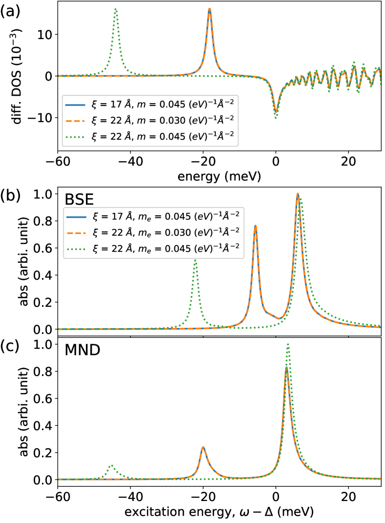
Figure 1: (a) Differential DOS; (b) Absorption spectrum from the BSE formalism; (c) Absorption spectrum from the MND theory with $\beta^{-1}=0$ meV, $\varepsilon_{\text{F}}=5$ meV, $\gamma=1$ meV, $N=140$.

In this section, we study the bound-state solution of the electron-exciton scattering problem by solving the eigenvalue problem

$$\sum_{\mathbf{k}^{\prime}}\left(\delta_{\mathbf{k},\mathbf{k}^{\prime}}\frac{|\mathbf{k}|^{2}}{2m}+V_{\mathbf{k},\mathbf{k}^{\prime}}\right)\Phi_{\mathbf{k}^{\prime},n}=\tilde{\varepsilon}_{n}\Phi_{\mathbf{k},n}.$$ (92)

The equation is identical to Eq. (61) in our discussion of the MND theory for $m=m_{\text{e}}$. The equation with $m=\overline{m}_{\text{T}}$ can also be used to find the eigenvalue and the eigenvector of Eq. (51) since the center-of-mass momentum can be decoupled as

$$\tilde{\varepsilon}_{n,\mathbf{Q}} = \tilde{\varepsilon}_{n}+\frac{|\mathbf{Q}|^{2}}{2M_{\text{T}}},\hskip 8.61108pt\Phi_{\mathbf{k};n,\mathbf{Q}}=\Phi_{\mathbf{k},n}.$$ (93)

In order to describe the impurity-induced bound states of the system, we define the differential density of states (diff. DOS) as

$$\Delta\rho(\omega) \equiv \frac{1}{N^{2}}\left[\sum_{n}\delta(\omega-\tilde{\varepsilon}_{n})-\sum_{\mathbf{k}}\delta(\omega-\varepsilon_{\mathbf{k}})\right].$$ (94)

This quantity measures the spectral density shift from the non-interacting Fermi gas to the reorganized Fermi gas due to the electron-exciton interaction. In Fig. 1 (a), the calculated diff. DOS with different values of the electron mass and exciton radius is shown. It is found that a negative energy weakly bound state exists for each parameter set. In the language employed in this work, the weakly bound state is assigned as the trion state. The trion binding energy depends on the mass and the exciton radius. It is found that the trion binding energy increases as the electron mass and exciton radius parameters increase.

In Fig. 1 (b), (c), the optical spectra given by (b) the BSE formalism and (c) the MND theory with electron mass $m_{\text{e}}=m$ are shown for different exciton radius. The peaks close to $\omega-\Delta\simeq{0}$ are assigned as exciton transitions and the additional peaks with lower energies are assigned as trion transitions. As can be seen, the trion binding energies calculated with the same parameters but by different methods are quite different. The binding energy calculated by the BSE formalism is consistently smaller than the one calculated by the MND theory. This occurs because that the binding energy given by the BSE formalism is calculated by diagonalizing Eq. (92) with $m=\overline{m}_{\text{T}}=2m_{\text{e}}/3$, while the binding energy given by the MND theory is calculated from the same equation with $m=m_{\text{e}}$. The binding energy obtained from the BSE formalism with $m_{\text{e}}=0.045\;(\text{eV})^{-1}\text{\AA}^{-2}$ is close to the binding energy of the MND theory with $m_{\text{e}}=0.030\;(\text{eV})^{-1}\text{\AA}^{-2}$. Since the electron mass can be found experimentally and is about $m_{\text{e}}=0.045\;(\text{eV})^{-1}\text{\AA}^{-2}$, we choose different exciton radii for different methods ($\xi=22$ Å  for BSE and $\xi=17$ Å  for MND) to adjust the binding energies to similar values. Through this adjustment, we can compare the optical spectra by the two methods and exclude the binding energy difference, thus enabling consideration of edge-singularity effects.

Note that we use an overestimate of the exciton radius for each method and still find an underestimate of the trion binding energy. For a monolayer TMDC, such as $\text{MoS}_{2}$, the exciton radius is about $10$ Å  and the trion binding energy is over $20$ meV based on the calculation of the three-particle Schrödinger equation modelberkelbach2013theory . The deviation is caused by some factors not considered in the present theory. First, we do not include the exchange energy in our model. The exchange energy can be described as the indistinguishability between the doping electron and the bound electron in the exciton. For the Schrödinger equation model, the exchange energy can be included by assuming that the variational wavefunction is symmetric to the exchange of the two electron degrees of freedom. Secondly, we do not consider the effect whereby the exciton transition energy relaxes to lower values due to the interaction with the doping electrons. Lastly, the electron-exciton scattering potential has been written by assuming that the exciton wavefunction is a 1s-orbital solution of the two-dimensional hydrogen atom. However, it is possible that there exists excited state orbitals that hybridize with the exciton wavefunction when the exciton interacts with doping electrons. All of these factors contribute to the observed deviations and are beyond the present discussion. We will leave these issues to a future study.

V.4 Doping-dependent optical spectra

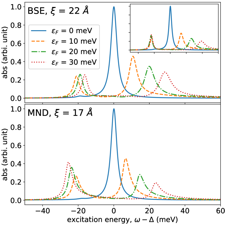
Figure 2: The doping-dependent optical spectra calculated by the BSE formalism (upper panel) and the MND theory (lower panel) with $m_{\text{e}}=0.045\;(\text{eV})^{-1}\text{\AA}^{-2}$, $\beta^{-1}=0.1$ meV, $\gamma=2$ meV, $N=140$. The inset in upper panel shows the spectra calculated by the BSE formalism without the distribution function of allowed transition $\rho_{n,\mathbf{Q}}$ for $n=0$ (the trion bound state) in Eq. (54).

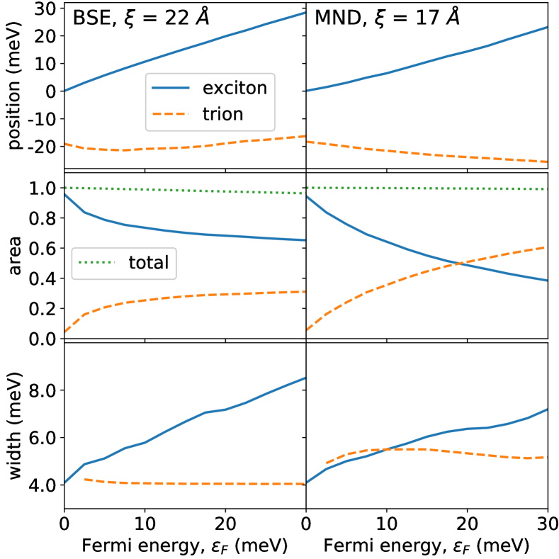
Figure 3: The doping-dependent exciton-trion peak positions, peak areas, and peak widths calculated by the BSE formalism (left) and the MND theory (right) with $m_{\text{e}}=0.045\;(\text{eV})^{-1}\text{\AA}^{-2}$, $\beta^{-1}=0.1$ meV, $\gamma=2$ meV, $N=140$. The peak areas are calculated by integrating the imaginary part of the exciton Green’s function, and are normalized to the total area at $\varepsilon_{\text{F}}=0$ for each method.

By altering the Fermi energy, the doping dependence of the optical spectrum can be studied. Fig. 2 shows the doping-dependent optical spectra calculated by both the BSE formalism and the MND theory. As can be seen, for both methods the trion peak emerges with positive Fermi energies, and the energy splitting between the exciton peak and the trion peak increases upon doping. The oscillator strength transfer from exciton peak to trion peak calculated by the BSE formalism saturates with increasing $\varepsilon_{\text{F}}$. The saturation can only be attributed partially to the Pauli-blocking effect discussed in Sec. IV.3. Via performing the BSE calculation without the distribution function of allowed transition $\rho_{n,\mathbf{Q}}$ for $n=0$ (the trion bound state) in Eq. (54), a new doping-dependent spectra is shown in the inset of Fig. 2 and a reduction of the saturation of the oscillator strength transfer is observed. The heights of the trion peaks in the high doping-density regime ($\varepsilon_{\text{F}}\geq\Delta_{\text{T}}$) surpass those of the exciton peaks. However, the peak area transfer between the exciton and trion peaks remains saturated. The result (the exceedance of the peak heights and the saturation of the peak areas) is consistent with the calculation of Refefimkin2017many , which also does not appear to contain explicit Pauli-blocking term for the trion transition. On the other hand, the oscillator strength transfer calculated by the MND theory shows no saturation.

Via simple curve fitting, the energy splitting between exciton peak and trion peak, the peak areas, and the peak widths of the two peaks calculated by the BSE formalism and the MND theory are estimated and shown in Fig. 3. For calculations based on the BSE formalism, the energy splitting is approximately proportional to the Fermi energy, $E_{\text{split}}\simeq\Delta_{\text{T}}+\varepsilon_{\text{F}}$, and $\Delta_{\text{T}}$ is about $19$ meV, where the trion binding energy is equal to the peak position of the Diff. DOS calculation shown in Fig. 1 (a) with $\xi=22\;\text{\AA}$ and $m=0.030\;\text{eV}^{-1}\text{\AA}^{-2}$. The increasing peak area of the trion transition and the decreasing peak area of the exciton transition with respect to increasing the Fermi energy are shown, and the total area is conserved for different Fermi energies. As can be seen in Fig. 3, the oscillator strength transfer is gradually saturated. For the peak widths, the exciton linewidth is roughly proportional to the Fermi energy, implying that the scattering potential is more similar to a contact potential at the relevant length scales. On the other hand, the trion linewidth is basically invariant to changes in the Fermi energy as found in Refefimkin2017many .

For the calculations based on the MND theory, the trion peak continues to grow as the Fermi energy increases, and the energy splitting is given by $E_{\text{split}}\simeq\Delta_{\text{T}}+\varepsilon_{\text{F}}$, with $\Delta_{\text{T}}$ about $19$ meV, where the trion binding energy is equal to the peak position of the Diff. DOS calculated in Fig. 1 (a) with $\xi=17\;\text{\AA}$ and $m=0.045\;\text{eV}^{-1}\text{\AA}^{-2}$. Note that the doping density is nonzero at $\varepsilon_{\text{F}}=0$ eV due to the small but non-zero temperature, such that the trion lineshape emerges and has a finite oscillator strength even at $\varepsilon_{\text{F}}=0$. Similar to the BSE calculation, with increasing Fermi energy the peak area of the trion transition increases and the peak area of the exciton transition decreases, with the total area conserved for different doping densities. The peak areas of exciton and trion transitions intersect around $18$ meV, which is also close to the trion binding energy. The peak widths of exciton and trion transitions are found to have a somewhat quantitatively different dependence with the Fermi energy. The trion linewidth calculated by the MND theory is roughly invariant to the Fermi energy, and the exciton linewidth is proportional to the Fermi energy, as in the BSE calculation.

In comparison with the results calculated by the BSE formalism, the MND results show better correspondence with at least some experiments which show an oscillator strength transfer that shows no sign of saturation with increasing $\varepsilon_{\text{F}}$kheng1993observation ; huard2000bound ; yang2015robust . This implies that the Fermi sea multiple-electron-hole excitations, which are responsible for the creation of the Fermi-edge singularity, may also contribute to the trion transition.

V.5 Temperature-dependent optical spectra

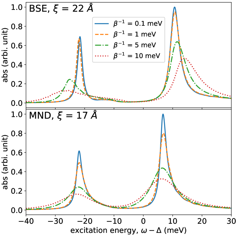
Figure 4: The temperature-dependent optical spectra calculated by the BSE formalism (upper panel) and the MND theory (lower panel) with $m_{\text{e}}=0.045\;(\text{eV})^{-1}\text{\AA}^{-2}$, $\varepsilon_{\text{F}}=10$ meV, $\gamma=1$ meV, $\varepsilon_{\Lambda}=2.0$ eV, $N=120$.

In this section, the temperature dependence of the optical spectrum is discussed. In Fig. 4, the temperature-dependent optical spectra calculated by both the BSE formalism and the MND theory are given. For both spectra, the linewidths are broadened and the peak-heights become lower as the temperature increases. For the spectra calculated by the MND theory in extremely low temperature regime (below $1$ meV), both the exciton and the trion peaks exhibit asymmetric lineshapes near the transition energies ($\omega-\Delta\simeq\mu$ for exciton and $\omega-\Delta\simeq-\Delta_{\text{T}}$ for trion), and the peak heights are sensitive to the temperature. Both of these features are signatures of the Fermi-edge singularity. On the other hand, the spectra calculated by the BSE formalism are relatively insensitive to temperature variations in this low temperature regime. As can be seen in Fig. 4, only very small variations of the trion and exciton lineshapes can be observed when the temperature is on the order of 5% of the trion binding energy.

VI Discussions and conclusion

In the present work, we have theoretically studied the problem of an exciton immersed in a Fermi sea which interacts with electrons through a scattering potential. We have focused on two approximate methods, the BSE formalism and the MND theory, to solve a many-body Hamiltonian parametrized to describe two-dimensional semiconductors. We find some results that are coincident with experimental observations and expectations. Both the BSE formalism and the MND theory describe the trion peak emergence, the oscillator strength transfer, and the doping-independent lineshapes in a sensible manner in the low doping-density regime. When the Fermi energy exceeds the trion binding energy, the BSE formalism may not account completely for the oscillator strength transfer from the exciton peak to the trion peak, while the MND theory is found to describe this effect. This limitation of the BSE approach can only be altered in part by the ad-hoc procedure of removing the Pauli-blocking term.

Neither the BSE nor the MND theories are expected to capture all experimental features over all parameter regimes, since they only describe two limiting physical situations of a simple model. Even if we could solve the many-body scattering Hamiltonian exactly, there are still many factors which are not included in our model which could affect the results of the calculations. In Sec. V.3 we have discussed three such factors that may result in an underestimation of the trion binding energy. The same missing physical ingredients may also cause errors in the prediction of the doping dependence and temperature dependence of optical spectra. In addition to the mentioned factors, a significant approximation of the many-body scattering Hamiltonian is that the Fermi sea is assumed to be composed of non-interacting electrons. This is not a particularly realistic assumption, since in two dimensions the long-range Coulomb interaction is not fully screened and thus electron correlation effects may be important. A direct consequence of electron correlation is that the electron mass, the exciton mass, and the scattering potential should be renormalized according to the Fermi energy and temperaturemahan2013many ; galitski2004universal ; zhang2005quasiparticle . Electron correlation can also affect the ratio between the electron mass and exciton mass, and alter the effective scattering potential, thus changing the trion binding energy and the absorption lineshapes. Without considering the renormalization induced by electron correlation, precise predictions are difficult to obtain. These issues are beyond the scope of the present work, and we leave the topic of electron-electron interactions in the optical spectra to a future study.

Despite the physical factors which we do not include, the present model and its approximate solutions still provide a qualitative description and a physically clear picture of the doping-dependent optical spectra in two-dimensional semiconductors. In a nutshell, trion formation can be realized as the dynamical generation of a trion and a hole in the Fermi sea. The dynamical process originates from the electron-hole polarization near the Fermi sea induced by electron-exciton interaction, with the trion state formed as the bound state of an electron-exciton scattering process. From the fundamental (electron/hole) particle point of view, the scattering event involves a four-particle generation process, with the participation of two electrons plus one hole in the conduction band, and one hole in the valence band. The wavefunction for the trion-hole state is coherently coupled with the exciton wavefunction, as the discussion in Sec. II. The coupling strength can be connected to the electron-exciton scattering potential. Recently, two-dimensional coherent spectra in quantum wellsmoody2014coherent and TMDCssingh2014coherent ; hao2016coherent ; shepard2017trion have been studied, and the role of coherent exciton-trion coupling has been discussed in the context of these experiments. Coherent coupling has been attributed to exciton-trion many-body interactionssingh2014coherent , but a microscopic theory of these interactions has not been put forward. The present theory supports the existence of such a coupling, and may provide a theoretical foundation for the study coherent multi-dimensional spectra in the future.

Note added - After this work was completed, we became aware of Ref.chang2018crossover which presents calculations related to, and several conclusions similar to, those found in this work.

References

- (1) K. Kheng, R. T. Cox, M. Y. d’Aubigné, F. Bassani, K. Saminadayar, and S. Tatarenko, Phys. Rev. Lett., 71, 1752 (1993).
- (2) V. Huard, R. T. Cox, K. Saminadayar, A. Arnoult, and S. Tatarenko, Phys. Rev. Lett., 84, 187 (2000).
- (3) G. V. Astakhov, V. P. Kochereshko, D. R. Yakovlev, W. Ossau, J. Nürnberger, W. Faschinger, and G. Landwehr, Phys. Rev. B, 62, 10345 (2000).
- (4) V. Ciulin, P. Kossacki, S. Haacke, J.-D. Ganiére, B. Deveaud, A. Esser, M. Kutrowski, and T. Wojtowicz, Phys. Rev. B, 62, R16310 (2000).
- (5) K. F. Mak, K. He, C. Lee, and G. H. Lee, J. Hone, T. F. Heinz, and J. Shan, Nature materials, 12, 207 (2013).
- (6) T. C. Berkelbach, M. S. Hybertsen, and D. R. Reichman, Phys. Rev. B, 88, 045318 (2013).
- (7) J. Yang, T. Lu, Y. W. Myint, J. Pei, D. Macdonald, J.-C. Zheng, and Y. Lu, ACS nano, 9, 6603 (2015).
- (8) T. C. Berkelbach, and D. R. Reichman, Ann. Rev. Condens. Matter Phys., 9, 379 (2018).
- (9) N. Akizuki, M. Iwamura, S. Mouri, Y. Miyauchi, T. Kawasaki, H. Watanabe, T. Suemoto, K. Watanabe, K. Asano, and K. Matsuda, Phys. Rev. B, 89, 195432 (2014).
- (10) H. Hartleb, F. Späth, and T. Hertel, ACS nano, 9, 10461 (2015).
- (11) A. E. Ruckenstein, and S. Schmitt-Rink, Phys. Rev. B, 35, 7551 (1987).
- (12) P. Hawrylak, Phys. Rev. B, 44, 3821 (1991).
- (13) S. A. Brown, J. F. Young, J. A. Brum, P. Hawrylak, and Z. Wasilewski, Phys. Rev. B, 54, R11082 (1996).
- (14) M. Combescot, and J. Tribollet, Solid State Commun., 128, 273 (2003).
- (15) M. Combescot, J. Tribollet, G. Karczewski, F. Bernardot, C. Testelin, and M. Chamarro, Europhys. Lett., 71, 431 (2005).
- (16) B. Stébé, E. Feddi, A. Ainane, and F. Dujardin, Phys. Rev. B, 58, 9926 (1998).
- (17) A. Esser, E. Runge, R. Zimmermann, W. Langbein, Phys. Rev. B, 62, 8232 (2000).
- (18) F. X. Bronold, Phys. Rev. B, 61, 12620 (2000).
- (19) A. Esser, R. Zimmermann, and Runge, phys, stat. sol. (b), 227, 317 (2001).
- (20) R. A. Suris, V. P. Kochereshko, G. V. Astakhov, D. R. Yakovlev, W. Ossau, J. Nur̈nberger, W. Faschinger, G. Landwehr, T. Wojtowicz, G. Karczewski, and J. Kossut, phys, stat. sol. (b), 227, 343 (2001).
- (21) W. J. Ossau, and R. Suris, Optical properties of 2D systems with interacting electrons, (Springer Science & Business Media, New York, 2012).
- (22) S.-Y. Shiau, M. Combescot, and Y.-C. Chang, Phys. Rev. B, 86, 115210 (2012).
- (23) M. Baeten, and M. Wouters, Phys. Rev. B, 91, 115313 (2015).
- (24) D. K. Efimkin, and A. H. MacDonald, Phys. Rev. B, 95, 035417 (2017).
- (25) M. Klawunn, and A. Recati, Phys. Rev. B, 84, 033607 (2011).
- (26) R. Schmidt, T. Enss, V. Pietilä and E. Demler, Phys. Rev. A, 85, 021602(R) (2012).
- (27) M. M. Parish, and J. Levinsen, Phys. Rev. A, 87, 033616 (2013).
- (28) P. Massignan, M. Zaccanti, and G. M. Bruun, Rep. Prog. Phys., 77, 034401 (2014).
- (29) G. D. Mahan, Phys. Rev., 163, 612 (1967).
- (30) P. Noziéres, and C. T. De Dominicis, Phys. Rev., 178, 1097 (1969).
- (31) J. Gavoret, P. Nozieres, B. Roulet, and M. Combescot, J. Phys., 30, 987 (1969).
- (32) M. Combescot, and P. Nozieres, J. Phys., 32, 913 (1971).
- (33) G. D. Mahan, Phys. Rev. B, 4, 1421 (1980).
- (34) U. von Barth, and G. Grossmann, Phys. Rev. B, 8, 5150 (1982).
- (35) G. D. Mahan, Many-particle physics, (Springer Science & Business Media, New York, 2013).
- (36) D. Pimenov, J. von Delft, L. Glazman, and M. Goldstein, Phys. Rev. B, 96, 155310 (2017).
- (37) R. Schmidt, M. Knap, D. A. Ivanov, J.-S. You, M. Cetina, and E. Demler, Rep. Prog. Phys., 81, 024401 (2018).
- (38) H. Haug, and S. W. Koch, Quantum Theory of the Optical and Electronic Properties of Semiconductors: Fivth Edition, (World Scientific Publishing Co. Pte. Ltd, Singapore, 2009).
- (39) B. A. Lippmann, and J. Schwinger, Phys. Rev., 79, 469 (1950).
- (40) J. R. Taylor, Scattering theory: the quantum theory of nonrelativistic collisions (Dover Publications, Inc., Mineola, New York, 2006).
- (41) A. Vagov, H. Schomerus, and A. Shanenko, Phys. Rev. B, 76, 214513 (2007).
- (42) B. R. Holstein, Am. J. Phys., 61, 142 (1992).
- (43) S.-L. Nyeo, Am. J. Phys., 68, 571 (2000).
- (44) N. S. Rytova, Vestn. Mosk. Univ. Fiz. Astron., 3, 30 (1967).
- (45) L. V. Keldysh, J. Exp. Theoret. Phys. Lett., 29, 658 (1979).
- (46) B. Liu, W. Zhao, Z. Ding, I. Verzhbitskiy, L. Li, J. Lu, J. Chen, G. Eda, and K. P. Loh, Adv. Mater., 28, 6457 (2016).
- (47) K. Yao, A. Yan, S. Kahn, A. Suslu, Y. Liang, E. S. Barnard, S. Tongay, A. Zettl, N. J. Borys, and P. J. Schuck, Phys. Rev. Lett., 119, 087401-1 (2017).
- (48) R. Zimmermann, K. Kilimann, W. D. Kraeft, D. Kremp, and G. Röpke, phys. stat. sol. (b), 90, 175 (1978).
- (49) S. Schmitt-Rink, and C. Ell, High Excitation and Short Pulse Phenomena, 585, (Elsevier, 1985).
- (50) J. C. Inkson, J. Phys. C: Solid State Physics, 9, 1177 (1976).
- (51) S. Gao, and L. Yang, Phys. Rev. B, 96, 155410 (2017).
- (52) F. Stern, Phys. Rev. Lett., 18, 546 (1967).
- (53) V. M. Galitski, and S. Das Sarma, Phys. Rev. B, 70, 035111 (2004).
- (54) Y. Zhang, and S. Das Sarma, Phys. Rev. B, 71, 045322 (2005).
- (55) G. Moody, I. A. Akimov, H. Li, R. Singh, D. R. Yakovlev, G. Karczewski, M. Wiater, T. Wojtowicz, M. Bayer, and S. T. Cundiff, Phys. Rev. Lett., 112, 097401 (2014).
- (56) A. Singh, G. Moody, S. Wu, Y. Wu, N. J. Ghimire, J. Yan, D. G. Mandrus, X. Xu, and X. Li, Phys. Rev. Lett., 112, 216804 (2014).
- (57) K. Hao, L. Xu, P. Nagler, A. Singh, K. Tran, C. K. Dass, C. Schuller, T. Korn, X. Li, and G. Moody, Nano lett., 16, 5109 (2016).
- (58) G. D. Shepard, J. V. Ardelean, O. A. Ajayi, D. Rhodes, X. Zhu, J. C. Hone, and S. Strauf, ACS nano, 11, 11550 (2017).
- (59) Y.-C. Chang, S.-Y. Shiau, and M. Combescot, arXiv:1810.13061v1.