Discrepancy in tidal deformability of GW170817 between the Advanced LIGO twin detectors

Abstract

We find that the Hanford and Livingston detectors of Advanced LIGO derive a distinct posterior probability distribution of binary tidal deformability $\tilde{\Lambda}$ of the first binary-neutron-star merger GW170817. By analyzing public data of GW170817 with a nested-sampling engine and the default TaylorF2 waveform provided by the LALInference package, the probability distribution of the binary tidal deformability derived by the LIGO-Virgo detector network turns out to be determined dominantly by the Hanford detector. Specifically, by imposing the flat prior on tidal deformability of individual stars, symmetric 90% credible intervals of $\tilde{\Lambda}$ are estimated to be $527^{+619}_{-345}$ with the Hanford detector, $927^{+522}_{-619}$ with the Livingston detector, and $455^{+668}_{-281}$ with the LIGO-Virgo detector network. Furthermore, the distribution derived by the Livingston detector changes irregularly when we vary the maximum frequency of the data used in the analysis. This feature is not observed for the Hanford detector. While they are all consistent, the discrepancy and irregular behavior suggest that an in-depth study of noise properties might improve our understanding of GW170817 and future events.

I Introduction

Tidal deformability of neutron stars can be a key quantity to understand the hitherto-unknown nature of supranuclear density matter (see Ref. Lattimer and Prakash (2016) for reviews). The relation between the mass and tidal deformability is uniquely determined by the neutron-star equation of state Harada (2001); Lindblom and Indik (2014) as is the mass–radius relation Lindblom (1992). Thus, simultaneous measurements of the mass and tidal deformability are eagerly desired, and gravitational waves from binary-neutron-star mergers give us a perfect opportunity. Once the mass–tidal deformability relation is understood accurately, binary neutron stars can be used as standard sirens to explore the expansion of the universe even in the absence of electromagnetic counterparts Messenger and Read (2012). Motivated by these facts, the influence of tidal deformability on gravitational waves from binary neutron stars has been studied vigorously in this decade Flanagan and Hinderer (2008); Damour and Nagar (2010); Vines et al. (2011); Damour et al. (2012); Hotokezaka et al. (2013); Read et al. (2013); Hinderer et al. (2016).

The direct detection of gravitational waves from a binary-neutron-star merger, GW170817, enabled us to measure the tidal deformability of a neutron star for the first time Abbott et al. (2017a). The LIGO-Virgo collaboration (LVC) reported an upper bound on the most influential combination of tidal deformability parameters of two neutron stars, the so-called binary tidal deformability $\tilde{\Lambda}$, to be $\lesssim 800$ (all the values in this paper refer to 90% credibility) in their discovery paper Abbott et al. (2017a) under the reasonable assumption of small neutron-star spins (later corrected to $\lesssim 900$ Abbott et al. (2019a)). Independent analysis in Ref. De et al. (2018) reported, e.g., $\tilde{\Lambda}=222^{+420}_{-138}$ with the flat prior on the mass of neutron stars and the reasonable assumption of a common, causal equation of state for both neutron stars. LVC also reported an updated highest-posterior-density interval, $\tilde{\Lambda}=300^{+420}_{-230}$ Abbott et al. (2019a) using sophisticated waveform models Dietrich et al. (2017, 2019) (see also Ref. Abbott et al. (2019b) for an update), and this is further restricted to $190^{+390}_{-120}$ if a common equation of state is assumed Abbott et al. (2018).

All these inferences are made by combining the output of Advanced LIGO twin detectors, i.e., the Hanford and Livingston detectors (and Advanced Virgo). It should be important to examine the extent to which results derived by individual detectors agree, particularly in the presence of a glitch near merger Abbott et al. (2017a). A study of p–g instability presented the posterior probability distribution of $\tilde{\Lambda}$ derived by individual detectors Abbott et al. (2019c), but this is estimated only by incorporating this effect and by allowing high spins, which broaden the distribution of $\tilde{\Lambda}$. Neither consistency nor discrepancy of the derived distribution is discussed.

In this paper, we present our independent analysis of GW170817 to show that the Advanced LIGO twin detectors derive a distinct posterior probability distribution of $\tilde{\Lambda}$ (and only for this quantity; see the Appendix). Although the 90% credible intervals of $\tilde{\Lambda}$ are nominally consistent between the twin detectors, the distribution derived by the Livingston detector tends to prefer larger values of $\tilde{\Lambda}$ than those reported in the literature. Close inspection of the distribution suggests that the difference between the twin detectors might not be purely statistical. Specifically, the distribution derived by the Livingston detector does not behave smoothly with respect to the variation of the maximum frequency of the data used for parameter estimation. This behavior is not expected from physics of tidal deformation and should be contrasted with that of the distribution derived by the Hanford detector. The discrepancy between the twin detectors presages a challenge for determining tidal deformability accurately in future detections.

II Parameter estimation

We perform a Bayesian parameter estimation of GW170817 for (1) the Hanford data (Hanford-only), (2) the Livingston data (Livingston-only), and (3) combined data of the twin detectors and Advanced Virgo (HLV) as in previous work Abbott et al. (2017a); De et al. (2018); Abbott et al. (2019b, a). The data of GW170817 are made public by LVC. The calibration error is taken into account by using the calibration uncertainty envelope release for GWTC-1. As far as we tested, results derived by the HLV data change very little when the data from Virgo are discarded, as expected from the small signal-to-noise ratio Abbott et al. (2017a).

Presuming that gravitational waves are detected in the relevant data, $s(t)$, we compute the posterior probability distribution of binary parameters $\boldsymbol{\theta}$ via

$$p(\boldsymbol{\theta}|s(t))\propto p(s(t)|\boldsymbol{\theta})p(\boldsymbol{\theta}),$$ (1)

where $p(s(t)|\boldsymbol{\theta})$ is the likelihood and $p(\boldsymbol{\theta})$ is the prior probability distribution. The parameters, $\boldsymbol{\theta}$, consist of two masses, (aligned components of) two spins, two tidal deformability parameters, the luminosity distance, the sky position, the binary inclination, the polarization angle, the coalescence time, and the coalescence phase Abbott et al. (2017a).

We employ the nested sampling Skilling (2006); Veitch and Vecchio (2010) for the practical analysis using an engine implemented in the public LALInference package Veitch et al. (2015), a part of LSC Algorithmic Library Suite. We checked that all the independent realizations of the nested-sampling chains derive consistent results. We also checked that Markov Chain Monte Carlo parameter estimation derive consistent results.

We evaluate the likelihood following the standard procedure (see, e.g., Refs. Jaranowski and Królak (2009); Creighton and Anderson (2011)) using the noise power spectrum derived by the relevant data using BayesWave (see Appendix A and Appendix B of Ref. Abbott et al. (2019b)). The noise is assumed to be stationary and Gaussian during the parameter estimation. Following previous work Abbott et al. (2017a); De et al. (2018), we adopt the restricted post-Newtonian TaylorF2 approximant as the waveform model (see Ref. Abbott et al. (2019a) and references therein). This choice facilitates comparisons with previous results. Because this approximant is implemented in LALInference, results presented in this work should not be affected by our own analysis method and should be easy to reproduce. The minimum frequency of the data used in the analysis is fixed to $23\text{\,}\mathrm{Hz}$, and the maximum frequency $f_{\mathrm{max}}$ is varied to investigate its influence on estimation of $\tilde{\Lambda}$. Because we truncate the TaylorF2 approximant above the frequency at the innermost stable circular orbit around a nonspinning black hole with its mass being equal to the total mass of the binary, the results become identical for $f_{\mathrm{max}}\gtrsim$1600\text{\,}\mathrm{Hz}$$. In this work, we represent them by $f_{\mathrm{max}}=$2048\text{\,}\mathrm{Hz}$$ for simplicity.

We caution that the inferred value of $\tilde{\Lambda}$ entails systematic errors associated with inaccuracy of the TaylorF2 approximant. While the systematic error is subdominant compared to the statistical error for GW170817 Abbott et al. (2019a), we are also conducting further analysis employing a sophisticated waveform model developed based on numerical-relativity simulations by the Kyoto group Kiuchi et al. (2017); Kawaguchi et al. (2018). Regarding the topic of this paper, preliminary results suggest that this model only enhances the discrepancy between the twin detectors. In particular, the posterior probability distribution derived by the HLV data begins to exhibit a multiply-peaked structure consistently with the LVC analysis performed employing other sophisticated waveform models Abbott et al. (2019a). These results will be presented in a separate publication focusing on the comparison among waveform models Narikawa et al. (prep).

The prior probability distribution is chosen to follow those adopted in the LVC analysis Abbott et al. (2019a), and we mention specific choices made in this work. The sky position is fixed to the location determined by optical followup observations Utsumi et al. (2017) to save the computational cost. We checked that this has a negligible impact on estimation of $\tilde{\Lambda}$. This is expected, because $\tilde{\Lambda}$ is determined entirely by the phase of gravitational waves, while the sky position affects only the amplitude (see also Refs. Abbott et al. (2017b); De et al. (2018)). It should be cautioned that the sky position cannot be determined to any accuracy by a single detector Fairhurst (2009) in the absence of electromagnetic information. The low-spin prior (see Ref. Abbott et al. (2019a)) is adopted for the neutron-star spins for simplicity. The prior of the tidal deformability is chosen to be flat in $[0:5000]$ for individual components. This choice neglects the underlying equation of state, and its appropriate incorporation will tighten the constraint on $\tilde{\Lambda}$ De et al. (2018); Abbott et al. (2018). If we impose the flat prior on $\tilde{\Lambda}$, the discrepancy between the twin detectors is alleviated but remains. This alleviation is reasonable, because the flat prior on $\tilde{\Lambda}$ gives weight to the low-$\tilde{\Lambda}$ region where the discrepancy is mild as we see below.

In this study, we focus primarily on the marginalized posterior probability distribution of $\tilde{\Lambda}$. For completeness, we present estimates of other parameters in the Appendix. The discrepancy between the Advanced LIGO twin detectors is not observed significantly for parameters other than binary tidal deformability.

III Posterior of tidal deformability

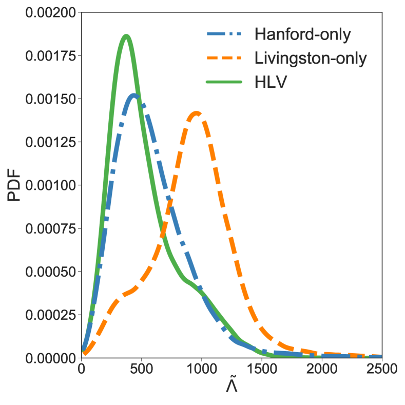
Figure 1: Marginalized posterior probability distribution of binary tidal deformability, $\tilde{\Lambda}$, derived by data of different detectors with $f_{\mathrm{max}}=$2048\text{\,}\mathrm{Hz}$$. The symmetric 90% credible intervals of $\tilde{\Lambda}$ for the Hanford-only data (blue) and the Livingston-only data (orange) are $\tilde{\Lambda}=527^{+619}_{-345}$ and $\tilde{\Lambda}=927^{+522}_{-619}$, respectively. The distribution obtained by combined data of Advanced LIGO twin detectors and Advanced Virgo (HLV, green) is closer to that derived by the Hanford-only data with its symmetric 90% credible interval being $\tilde{\Lambda}=455^{+668}_{-281}$.

Table 1: 90% credible interval of binary tidal deformability, $\tilde{\Lambda}$, for different data and the maximum frequency, $f_{\mathrm{max}}$. The upper group shows the symmetric intervals, and the lower shows the highest-posterior-density intervals, where the median is shown as a representative value for both groups.

$f_{\mathrm{max}}$	Hanford-only	Livingston-only	HLV
Symmetric interval
$800\text{\,}\mathrm{Hz}$	$1109^{+860}_{-798}$	$1023^{+750}_{-613}$	$988^{+591}_{-556}$
$900\text{\,}\mathrm{Hz}$	$667^{+651}_{-461}$	$913^{+729}_{-543}$	$671^{+489}_{-400}$
$1000\text{\,}\mathrm{Hz}$	$598^{+613}_{-413}$	$853^{+627}_{-479}$	$660^{+461}_{-384}$
$1100\text{\,}\mathrm{Hz}$	$636^{+566}_{-423}$	$785^{+601}_{-433}$	$659^{+397}_{-351}$
$1200\text{\,}\mathrm{Hz}$	$573^{+564}_{-372}$	$823^{+620}_{-449}$	$594^{+500}_{-362}$
$1300\text{\,}\mathrm{Hz}$	$579^{+543}_{-372}$	$889^{+573}_{-572}$	$521^{+557}_{-288}$
$1400\text{\,}\mathrm{Hz}$	$540^{+598}_{-342}$	$923^{+533}_{-611}$	$480^{+657}_{-280}$
$1500\text{\,}\mathrm{Hz}$	$526^{+627}_{-325}$	$925^{+526}_{-634}$	$438^{+655}_{-253}$
$2048\text{\,}\mathrm{Hz}$	$527^{+619}_{-345}$	$927^{+522}_{-619}$	$455^{+668}_{-281}$
Highest posterior density interval
$800\text{\,}\mathrm{Hz}$	$1109^{+797}_{-857}$	$1023^{+681}_{-677}$	$988^{+574}_{-577}$
$900\text{\,}\mathrm{Hz}$	$667^{+556}_{-529}$	$913^{+632}_{-620}$	$671^{+451}_{-437}$
$1000\text{\,}\mathrm{Hz}$	$598^{+508}_{-479}$	$853^{+549}_{-543}$	$660^{+424}_{-417}$
$1100\text{\,}\mathrm{Hz}$	$636^{+484}_{-487}$	$785^{+522}_{-495}$	$659^{+378}_{-369}$
$1200\text{\,}\mathrm{Hz}$	$573^{+451}_{-443}$	$823^{+530}_{-519}$	$594^{+444}_{-409}$
$1300\text{\,}\mathrm{Hz}$	$579^{+438}_{-437}$	$889^{+524}_{-615}$	$521^{+422}_{-362}$
$1400\text{\,}\mathrm{Hz}$	$540^{+485}_{-410}$	$923^{+468}_{-665}$	$480^{+541}_{-351}$
$1500\text{\,}\mathrm{Hz}$	$526^{+505}_{-399}$	$925^{+467}_{-684}$	$438^{+546}_{-320}$
$2048\text{\,}\mathrm{Hz}$	$527^{+498}_{-419}$	$927^{+467}_{-666}$	$455^{+562}_{-349}$

Figure 1 shows the marginalized posterior probability distribution of binary tidal deformability, $\tilde{\Lambda}$, derived by the Hanford-only data, Livingston-only data, and combined HLV data with $f_{\mathrm{max}}=$2048\text{\,}\mathrm{Hz}$$. The corresponding 90% credible intervals are presented in Table 1. The HLV distribution exhibits a peak at $\tilde{\Lambda}\approx 370$ with a tail extending to the high-$\tilde{\Lambda}$ region consistently with previous work De et al. (2018); Abbott et al. (2019a). Estimates of other parameters are also broadly consistent with those derived in previous work (see the Appendix).

The separate analysis of the data obtained by the individual of twin detectors reveals a mild discrepancy between them. On the one hand, the posterior probability distribution derived by the Hanford-only data is similar to that derived by the HLV data. It exhibits a peak at $\tilde{\Lambda}\approx 440$ with a tail at the high-$\tilde{\Lambda}$ region. Because the tail structure is enhanced for the HLV data due to the Livingston detector as we discuss below, the 90% credible intervals are similar for these two distributions (see Table 1). On the other hand, the distribution derived by the Livingston-only data peaks at a large value of $\tilde{\Lambda}\approx 960$, which is close to the edge of the 90% credible intervals of either the Hanford-only or HLV distribution. Conversely, the Livingston-only distribution has a small probability around $\tilde{\Lambda}\approx 400$.

We find that the HLV distribution is approximately reproduced by multiplying the Hanford-only distribution and the Livingston-only distribution if we appropriately incorporate the prior probability distribution of $\tilde{\Lambda}$ determined by that of other parameters. Specifically, we need to divide the multiplied distribution by the prior, because it is included in both the Hanford-only and Livingston-only distributions. The division by the prior reduces the probability at the high-$\tilde{\Lambda}$ region, and thus the data of the Livingston detector have a minor influence on the combined result. Still, the HLV distribution shows a bump at $\tilde{\Lambda}\approx 1000$ inherited from the peak of the Livingston-only distribution.

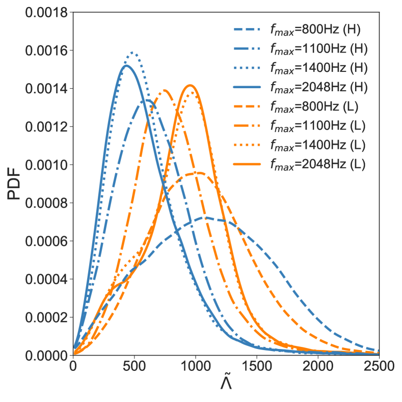
Figure 2: Dependence of the marginalized posterior probability distribution on the maximum frequency, $f_{\mathrm{max}}$, imposed in the data analysis. We adopt $f_{\mathrm{max}}=800$, 1100, 1400, and $2048\text{\,}\mathrm{Hz}$. While the distribution derived by the Hanford-only data (blue, denoted by H) shifts smoothly to the low-$\tilde{\Lambda}$ region as $f_{\mathrm{max}}$ increases, that by the Livingston-only data (orange, denoted by L) shows a turn at $f_{\mathrm{max}}\approx$1100\text{\,}\mathrm{Hz}$$.

Detailed features of the data from individual detectors are clarified by examining changes of the posterior probability distribution with respect to the variation of the maximum frequency, $f_{\mathrm{max}}$, imposed in the data analysis. Figure 2 shows the results for $f_{\mathrm{max}}=800$, 1100, 1400, and $2048\text{\,}\mathrm{Hz}$ (the same as Fig. 1). The Hanford-only distribution shifts smoothly to the low-$\tilde{\Lambda}$ region as $f_{\mathrm{max}}$ increases, and the median value decreases approximately monotonically. This is reasonably expected, because the tidal deformability is primarily determined by the gravitational-wave data at high frequency Damour et al. (2012); De et al. (2018). This feature results from the nature of tidal interaction and does not rely on complicated relativistic effects.

On another front, the posterior probability distribution derived by the Livingston-only data shows irregular behavior with respect to the increase of $f_{\mathrm{max}}$. At the beginning, the distribution shifts to the low-$\tilde{\Lambda}$ region in a similar manner to the Hanford-only distribution when $f_{\mathrm{max}}$ is decreased from $800\text{\,}\mathrm{Hz}$. However, the shift turns around at $f_{\mathrm{max}}\approx$1100\text{\,}\mathrm{Hz}$$, and then the distribution moves back to the high-$\tilde{\Lambda}$ region. The median values presented in Table 1 clearly exhibit the turn, and neither a systematic decrease nor increase is observed. This is not naturally anticipated from the viewpoint of measurability Damour et al. (2012); De et al. (2018).

Taking the fact that the distribution of $\tilde{\Lambda}$ obtained by the combined HLV data is similar to that by the Hanford-only data into account, the peculiar dependence on $f_{\mathrm{max}}$ might indicate that the high-frequency data of the Livingston detector are not very helpful to determine $\tilde{\Lambda}$ of GW170817. Note that the signal-to-noise ratio is larger for Livingston than for Hanford due to the higher sensitivity Abbott et al. (2017a, 2019a). Specifically, the signal-to-noise ratios derived in our analysis are 18.8, 26.8, and 32.6 for Hanford, Livingston, and HLV, respectively. Thus, the dominance of Hanford data in the combined result is not reasonably understood from the signal-to-noise ratio. Actually, we find that the posterior probability distributions of other parameters are more strongly influenced by Livingston than Hanford (see the Appendix).

A careful examination of Fig. 2 reveals that a small bump appears for $f_{\mathrm{max}}\gtrsim$1400\text{\,}\mathrm{Hz}$$ at the low-$\tilde{\Lambda}$ region of the posterior probability distribution derived by the Livingston-only data. The location of this bump is close to the peak of $\tilde{\Lambda}$ derived by the Hanford-only data. Thus, the Livingston-only distribution may consist of the main peak with a large value of $\tilde{\Lambda}$ associated with the low-frequency data and the side peak with a small value of $\tilde{\Lambda}$ associated with the high-frequency data.

IV Discussion

Our analysis suggests that the noise in the high-frequency region of the Livingston data somehow corrupted information about the tidal deformability of GW170817. Although this could simply be caused by the stationary and Gaussian noise, it could be worthwhile to look for possible peculiar features in the data of GW170817, e.g., a residual of the glitch in the Livingston data at about a half second before merger Abbott et al. (2017a) (but see also Ref. Pankow et al. (2018)) as it is quite important to estimate tidal deformability accurately. By contrast, the Hanford data seem to be well-behaved during the reception of GW170817.

Having said that, it is ultimately impossible to judge which of the Advanced LIGO twin detectors provides us with a more reliable estimate of the binary tidal deformability than the other does, or whether simply their combination is the most reliable, without meaningful data obtained by a third detector. It should be emphasized that the 90% credible intervals are consistent between the twin detectors. What we may safely conclude is that the posterior probability distribution is exceptionally distinct for binary tidal deformability (see the Appendix for other parameters) and that the Livingston data are not very useful for constraining its value in the case of GW170817. Secure parameter estimation will be helped by unambiguous detection by other instruments such as Advanced Virgo or KAGRA Abbott et al. (2016). However, if the irregular loss of information is typical for detections with a moderate signal-to-noise ratio, accurate determination of tidal deformability will remain challenging unless its origin is identified.

Appendix A Parameter other than tidal deformability

Table 2: 90% credible interval of the luminosity distance, the binary inclination, mass parameters, and the effective spin parameter derived by different data with $f_{\mathrm{max}}=$2048\text{\,}\mathrm{Hz}$$. We show 10%–100% regions of the mass ratio with the upper limit $q=1$ imposed by the prior, and those of $m_{1}$ and $m_{2}$ are given accordingly. We give symmetric 90% credible intervals, i.e., 5%–95%, for the other parameters with the median as a representative value. The binary inclination derived by either the Hanford-only or Livingston-only data is undetermined up to the orbital-plane reflection, and thus the 90% credible interval is very large.

	Hanford-only	Livingston-only	HLV
Luminosity distance $d_{L}~{}[$\mathrm{M}\mathrm{p}\mathrm{c}$]$	$40.8^{+10.3}_{-17.1}$	$39.0^{+9.0}_{-16.4}$	$41.0^{+7.7}_{-15.2}$
Binary inclination $\theta_{\mathrm{JN}}$ [degree]	$88^{+77}_{-74}$	$86^{+79}_{-72}$	$146^{+24}_{-28}$
Chirp mass in the detector frame $\mathcal{M}^{\mathrm{det}}~{}[M_{\odot}]$	$1.1978^{+0.0002}_{-0.0002}$	$1.1975^{+0.0001}_{-0.0001}$	$1.1975^{+0.0001}_{-0.0001}$
Chirp mass in the source frame $\mathcal{M}~{}[M_{\odot}]$	$1.187^{+0.005}_{-0.003}$	$1.187^{+0.004}_{-0.002}$	$1.187^{+0.004}_{-0.002}$
Primary mass $m_{1}~{}[M_{\odot}]$	(1.36, 1.56)	(1.36, 1.59)	(1.36, 1.59)
Secondary mass $m_{2}~{}[M_{\odot}]$	(1.20, 1.37)	(1.17, 1.37)	(1.17, 1.37)
Total mass $M_{\mathrm{tot}}:=m_{1}+m_{2}~{}[M_{\odot}]$	$2.73^{+0.03}_{-0.01}$	$2.74^{+0.04}_{-0.01}$	$2.74^{+0.04}_{-0.01}$
Mass ratio $q:=m_{2}/m_{1}$	(0.77, 1)	(0.74, 1)	(0.74, 1)
Effective spin $\chi_{\mathrm{eff}}$	$0.014^{+0.010}_{-0.011}$	$0.003^{+0.015}_{-0.010}$	$0.002^{+0.015}_{-0.009}$

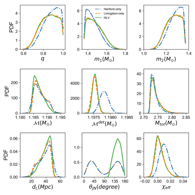
Figure 3: Marginalized posterior probability distribution of various parameters with $f_{\mathrm{max}}=$2048\text{\,}\mathrm{Hz}$$. The blue, orange, and green curves correspond to the Hanford-only, Livingston-only, and HLV data, respectively. The top-left, top-middle, top-right, middle-left, center, middle-right, bottom-left, bottom-middle, and bottom-right panels show $q$, $m_{1}$, $m_{2}$, $\mathcal{M}$, $\mathcal{M}^{\mathrm{det}}$, $M_{\mathrm{tot}}$, $d_{L}$, $\theta_{\mathrm{JN}}$, and $\chi_{\mathrm{eff}}$, respectively (see Table 2 for the definition of quantities). The distribution of $\theta_{\mathrm{JN}}$ for a single-detector data exhibits a bimodal structure due to the degeneracy of the orbital-plane reflection, and this is resolved for the HLV data.

We present estimates of parameters other than binary tidal deformability with $f_{\mathrm{max}}=$2048\text{\,}\mathrm{Hz}$$ for completeness. Table 2 presents the 90% credible intervals of the luminosity distance, the binary inclination, mass parameters, and the effective spin parameter derived by different data. We recall that the sky location is fixed by the information from electromagnetic observations and that the low-spin prior is imposed. The cosmological redshift is not taken from the host galaxy NGC4993 Abbott et al. (2017b) and is determined from the luminosity distance by assuming the Hubble constant $H_{0}=$69\text{\,}\mathrm{k}\mathrm{m}\,\mathrm{s}^{-1}\,\mathrm{M}\mathrm{p}\mathrm{c}^{-1}$$ (a default value in LAL) to derive the chirp mass in the source frame. The marginalized posterior distribution is presented in Fig. 3. The consistency of our results with previous work De et al. (2018); Abbott et al. (2019a) serves as an important sanity check. They also clarify that the estimation of binary tidal deformability is exceptionally delicate for GW170817.

Table 2 shows that the credible intervals agree remarkably between the Hanford-only and Livingston-only data. The marginalized posterior probability distribution depicted in Fig. 3 not only confirms this agreement but also shows that the distribution is approximately identical. The parameters shown here are estimated primarily from information at low frequency, where the gravitational-wave signal spends most of time with a large number of cycles Damour et al. (2012); De et al. (2018). The detector noise is also less severe at lower frequency. As a result, the situation is different from that of binary tidal deformability discussed in the main text.

The 90% credible intervals derived by combining the HLV data are very close to those of a single detector (Hanford-only or Livingston-only) except for the binary inclination, $\theta_{\mathrm{JN}}$. The reason for the difference in $\theta_{\mathrm{JN}}$ is that the degeneracy of the reflection with respect to the orbital plane, i.e., face-on or face-off, is resolved when the HLV data are combined. The resolution is clearly shown in the middle panel of the bottom row of Fig. 3, where the bimodal structure for a single detector is changed to a single peak for the HLV data favoring the face-off orientation. The posterior probability distribution of other parameters shifts only moderately.

Close inspection reveals that the posterior probability distribution derived by the HLV data closely follows that of the Livingston-only data for the chirp mass in the detector frame, the mass ratio, and the effective spin. Because they are determined by the gravitational-wave phase at low frequency, the closeness of the distribution can be understood as a result of the large signal-to-noise ratio for the Livingston detector. Again, these features are different from what we observe for the binary tidal deformability, where the distribution derived by the HLV data is closer to that derived by the Hanford-only data than the Livingston-only data.

References

- Lattimer and Prakash (2016) J. M. Lattimer and M. Prakash, Phys. Rep. 621, 127 (2016).
- Harada (2001) T. Harada, Phys. Rev. C 64, 048801 (2001).
- Lindblom and Indik (2014) L. Lindblom and N. M. Indik, Phys. Rev. D 89, 064003 (2014).
- Lindblom (1992) L. Lindblom, Astrophys. J. 398, 569 (1992).
- Messenger and Read (2012) C. Messenger and J. Read, Phys. Rev. Lett. 108, 091101 (2012).
- Flanagan and Hinderer (2008) É. É. Flanagan and T. Hinderer, Phys. Rev. D 77, 021502 (2008).
- Damour and Nagar (2010) T. Damour and A. Nagar, Phys. Rev. D 81, 084016 (2010).
- Vines et al. (2011) J. Vines, É. É. Flanagan, and T. Hinderer, Phys. Rev. D 83, 084051 (2011).
- Damour et al. (2012) T. Damour, A. Nagar, and L. Villain, Phys. Rev. D 85, 123007 (2012).
- Hotokezaka et al. (2013) K. Hotokezaka, K. Kyutoku, and M. Shibata, Phys. Rev. D 87, 044001 (2013).
- Read et al. (2013) J. S. Read, L. Baiotti, J. D. E. Creighton, J. L. Friedman, B. Giacomazzo, K. Kyutoku, C. Markakis, L. Rezzolla, M. Shibata, and K. Taniguchi, Phys. Rev. D 88, 044042 (2013).
- Hinderer et al. (2016) T. Hinderer, A. Taracchini, F. Foucart, A. Buonanno, J. Steinhoff, M. Duez, L. E. Kidder, H. P. Pfeiffer, M. A. Scheel, B. Szilagyi, K. Hotokezaka, K. Kyutoku, M. Shibata, and C. W. Carpenter, Phys. Rev. Lett. 116, 181101 (2016).
- Abbott et al. (2017a) B. P. Abbott, R. Abbott, T. D. Abbott, F. Acernese, K. Ackley, C. Adams, T. Adams, P. Addesso, R. X. Adhikari, V. B. Adya, and et al., Phys. Rev. Lett. 119, 161101 (2017a).
- Abbott et al. (2019a) B. P. Abbott, R. Abbott, T. D. Abbott, F. Acernese, K. Ackley, C. Adams, T. Adams, P. Addesso, R. X. Adhikari, V. B. Adya, and et al., Phys. Rev. X 9, 011001 (2019a).
- De et al. (2018) S. De, D. Finstad, J. M. Lattimer, D. A. Brown, E. Berger, and C. M. Biwer, Phys. Rev. Lett. 121, 091102 (2018).
- Dietrich et al. (2017) T. Dietrich, S. Bernuzzi, and W. Tichy, Phys. Rev. D 96, 121501 (2017).
- Dietrich et al. (2019) T. Dietrich, S. Khan, R. Dudi, S. J. Kapadia, P. Kumar, A. Nagar, F. Ohme, F. Pannarale, A. Samajdar, S. Bernuzzi, G. Carullo, W. D. Pozzo, M. Haney, C. Markakis, M. Pürrer, G. Riemenschneider, Y. Eka Setyawati, K. W. Tsang, and C. Van Den Broeck, Phys. Rev. D 99, 024029 (2019).
- Abbott et al. (2019b) B. P. Abbott, R. Abbott, T. D. Abbott, F. Acernese, K. Ackley, C. Adams, T. Adams, P. Addesso, R. X. Adhikari, V. B. Adya, and et al., Phys. Rev. X 9, 031040 (2019b).
- Abbott et al. (2018) B. P. Abbott, R. Abbott, T. D. Abbott, F. Acernese, K. Ackley, C. Adams, T. Adams, P. Addesso, R. X. Adhikari, V. B. Adya, and et al., Phys. Rev. Lett. 121, 161101 (2018).
- Abbott et al. (2019c) B. P. Abbott, R. Abbott, T. D. Abbott, F. Acernese, K. Ackley, C. Adams, T. Adams, P. Addesso, R. X. Adhikari, V. B. Adya, and et al., Phys. Rev. Lett. 122, 061104 (2019c).
- Skilling (2006) J. Skilling, Bayesian Analysis 1, 833 (2006).
- Veitch and Vecchio (2010) J. Veitch and A. Vecchio, Phys. Rev. D 81, 062003 (2010).
- Veitch et al. (2015) J. Veitch, V. Raymond, B. Farr, W. Farr, P. Graff, S. Vitale, B. Aylott, K. Blackburn, N. Christensen, M. Coughlin, W. Del Pozzo, F. Feroz, J. Gair, C.-J. Haster, V. Kalogera, T. Littenberg, I. Mandel, R. O’Shaughnessy, M. Pitkin, C. Rodriguez, C. Röver, T. Sidery, R. Smith, M. Van Der Sluys, A. Vecchio, W. Vousden, and L. Wade, Phys. Rev. D 91, 042003 (2015).
- Jaranowski and Królak (2009) P. Jaranowski and A. Królak, Analysis of gravitational-wave data (Cambridge University Press, 2009).
- Creighton and Anderson (2011) J. D. E. Creighton and W. G. Anderson, Gravitational-wave physics and astronomy: an introduction to theory, experiment and data analysys (Wiley-VCH, 2011).
- Kiuchi et al. (2017) K. Kiuchi, K. Kawaguchi, K. Kyutoku, Y. Sekiguchi, M. Shibata, and K. Taniguchi, Phys. Rev. D 96, 084060 (2017).
- Kawaguchi et al. (2018) K. Kawaguchi, K. Kiuchi, K. Kyutoku, Y. Sekiguchi, M. Shibata, and K. Taniguchi, Phys. Rev. D 97, 044044 (2018).
- Narikawa et al. (prep) T. Narikawa, N. Uchikata, K. Kawaguchi, K. Kiuchi, K. Kyutoku, M. Shibata, and H. Tagoshi, (in prep.).
- Utsumi et al. (2017) Y. Utsumi, M. Tanaka, N. Tominaga, M. Yoshida, S. Barway, T. Nagayama, T. Zenko, K. Aoki, T. Fujiyoshi, H. Furusawa, and et al., Publications of the Astronomical Society of Japan 69, 101 (2017).
- Abbott et al. (2017b) B. P. Abbott, R. Abbott, T. D. Abbott, F. Acernese, K. Ackley, C. Adams, T. Adams, P. Addesso, R. X. Adhikari, V. B. Adya, and et al., Nature (London) 551, 85 (2017b).
- Fairhurst (2009) S. Fairhurst, New Journal of Physics 11, 123006 (2009).
- Pankow et al. (2018) C. Pankow, K. Chatziioannou, E. A. Chase, T. B. Littenberg, M. Evans, J. McIver, N. J. Cornish, C.-J. Haster, J. Kanner, V. Raymond, S. Vitale, , and A. Zimmerman, Phys. Rev. D 98, 084016 (2018).
- Abbott et al. (2016) B. P. Abbott, R. Abbott, T. D. Abbott, M. R. Abernathy, F. Acernese, K. Ackley, C. Adams, T. Adams, P. Addesso, R. X. Adhikari, and et al., Living Reviews in Relativity 19, 1 (2016).