Revisiting the hardening of the stellar ionizing radiation in galaxy discs

Abstract

In this work we explore accurate new ways to derive the ionization parameter ($U$) and the equivalent effective temperature ($T_{*}$) in H ii regions using emission-line intensities from the ionized gas. The so-called softness parameter ($\eta$), based on [O ii], [O iii], [S ii], and [S iii] has been proposed to estimate the hardening of the ionizing incident field of radiation, but the simplest relation of this parameter with $T_{*}$ also depends on $U$ and metallicity ($Z$). Here we provide a Bayesian-like code (HCm-Teff) that compares the observed emission lines of $\eta$ with the predictions of a large grid of photoionization models giving precise estimations of both $U$ and $T_{*}$ when $Z$ is known. We also study the radial variation of these parameters in well-studied disc galaxies observed by the chaos collaboration. Our results indicate that the observed radial decreasing of $\eta$ can be attributed to a radial hardening of $T_{*}$, across galactic discs as in NGC 628 and NGC 5457. On the other hand NGC 5194, which presents a positive slope of the fitting of the softness parameter, has a flat slope in $T_{*}$. On the contrary the three galaxies do not seem to present large radial variations of the ionization parameter. When we inspect a larger sample of galaxies we observe steeper radial variations of $T_{*}$ in less bright and later-type galaxies, mimicking a similar trend observed for $Z$ but the studied sample should be enlarged to obtain more statistically significant conclusions.

1 Introduction

Objects whose luminosity is dominated by conspicuous emission lines from ionized gas are preferential targets in galaxies for the determination of many different physical properties of the spatial regions where they are located. Though the weighted average of the ionic species heavier than helium is usually lower than 2%, the relative intensity of the optical lines emitted by these elements is easily detectable in bright star-forming complexes. In the case of those elements that present more than one collisionally excited emission line corresponding to different ionization stages in the same spectral observed range, their study allows us to extract important conclusions about the photoionization equilibrium between the hardening of the ionizing radiation from massive stars and the density of elements in the surrounding gas.

According to McCall et al. (1985) most of the properties of the integrated emitting spectrum depend on three properties or so-called functional parameters: metallicity ($Z$), ionization parameter ($U$), and equivalent effective temperature ($T_{*}$). $Z$ is usually derived by means of measurement of the electron temperature using collisionally excited emission lines from one ion whose energies are similar (e.g. [O iii] 5007/4363). Alternatively, when no auroral emission line can be measured with enough confidence in the emission-line spectrum, we can resort to direct calibrations of the strong emission lines. $U$ can be estimated using ratios of emission lines corresponding to consecutive ionization stages, such as [O ii]/[O iii] and [S ii]/[S iii], although these ratios usually also present a strong additional dependence on the other functional parameters (e.g. Díaz 1998; Dors & Copetti 2003).

To calculate $T_{*}$ several authors have proposed different sensitive emission-line ratios, such as [Neiii] 3869 Å/H$\beta$ (Oey et al., 2000) and Hei/H$\beta$ (Vale Asari et al., 2016). Vilchez & Pagel (1988) proposed the use of two different ionic abundance ratios of consecutive ionization stages corresponding to species with very different excitation energies to trace the shape of the spectral ionizing energy distribution (SED). In the case of the optical range this can be obtained using oxygen and sulphur abundances that define the so-called softness parameter:

$$\eta=\frac{O^{+}/O^{2+}}{S^{+}/S^{2+}}$$ (1)

The softness parameter decreases at high $T_{*}$ of the field of radiation while it increases for low values of $T_{*}$.

These authors also defined the corresponding electron-temperature-independent line ratio quotient as:

$$\eta\prime=\frac{[OII]3727/[OIII]4959,5007}{[SII]6717,6731/[SIII]9059,9532}$$ (2)

Other authors have also proposed other sets of lines both in the optical (e.g. [Ariii]/[Ariv] vs [O ii]/[O iii]; Stasińska et al. 2015) and in the mid-infrared (e.g. [Neii]/[Neiii] vs [Siii]/[Siv]; Morisset 2004; Pérez-Montero & Vílchez 2009).

The use of this variant of the softness parameter based only on emission lines presents additional dependence on both $Z$ and $U$ (e.g. Morisset 2004). In addition a direct comparison between log $\eta\prime$ and $T_{*}$ of the field of radiation can result in uncertainty because the curves of equal $T_{*}$ predicted by single-star photoionization models have slopes lower than 1 in the plane log([S ii]/[S iii]) vs log([O ii]/[O iii]), so a spatial variation of $\eta\prime$ can also involve a variation of $U$ (e.g. Pérez-Montero et al. 2011; Fernández-Martín et al. 2017). In this way, Pérez-Montero et al. (2014) show in a 3D modelling of the giant H ii region NGC 595 that it can be predicted by a radial variation of log $\eta\prime$ only owing to the decrease of $U$ even if the ionizing central source is the same for all layers of the ionized gas. Therefore, it is necessary to provide new and more accurate recipes to give a trustable estimation of $T_{*}$ using the available optical emission lines.

One of the open issues on which a thorough study of the spatial variation of $T_{*}$ can shed some light is the radial variation of the functional parameters across spiral discs, which would help to constrain models of formation and build-up of these structures along cosmic time. From Searle (1971), it is known that there is a general trend to find higher excitations of the gas at larger galactocentric distances. This was soon linked with the presence of a decreasing radial variation of $Z$ (Smith 1975). The slope of these gradients correlates with the mass and luminosity of galaxies (e.g. Garnett et al. 1997; Pilyugin et al. 2004). The resulting slopes of the obtained fittings can even be normalized by the effective radius (Diaz, 1989), which can ease the study of the global radial variation of properties such as the total oxygen abundance (e.g. Sánchez et al. 2014) and the nitrogen-to-oxygen ratio (Pérez-Montero et al., 2016).

From the point of view of radial variation across galactic discs of $T_{*}$, Shields & Searle (1978) were the first to propose a radial enhancement in NGC 5457 based on the higher equivalent widths of H$\beta$ observed in the outermost H ii regions. Several authors have confirmed this trend in other spiral galaxies by means of a direct comparison between emission-line fluxes and photoionization models (e.g. Fierro et al. 1986; Dors & Copetti 2005; Dors et al. 2017. On the other hand this radial variation of $T_{*}$ with galactocentric distance is not apparently appreciated in the Milky Way (Morisset, 2004).

Pérez-Montero & Vílchez (2009) also measured a radial variation of the softness parameter in different disc galaxies. Most of the studied objects present lower values of $\eta\prime$ at larger galactocentric distances, which could be interpreted as a hardening of the ionizing stellar radiation across galactic discs. As in the case of $Z$ the scale of this variation seems to be related to the size and mass of the studied galaxies, though the sample of studied objects is still quite limited to establish solid conclusions in this respect. Therefore applying a new thorough analysis to a more complete sample of H ii regions in well-characterized galaxies would supply some clarification to the existence of gradients of one or various of the functional parameters in discs along with a possible connection between them and with other integrated properties of galaxies, as in the case of metallicity.

In this paper we present a new routine based on photoionization models to break the degeneracy of the softness parameter when it is calculated from emission lines and hence to provide precise estimates of both $U$ and $T_{*}$ in regions whose metallicity has been previously very well defined and with accurate measurements of the four optical emission lines involved in the calculation of $\eta\prime$. Our objective is to apply it to a sample of galaxies to study the radial variation of the derived properties and to verify whether the observed radial variation of the softness parameter can be attributed to a real variation of the hardening of the incident field of radiation across galactic discs.

The paper is organized as follows. In Section 2 we describe the new routine to obtain $U$ and $T_{*}$ using the emission lines involved in the definition of the softness parameter with the help of a large grid of photoionization models. Section 3 is devoted to comparing the results from this code with other models for both single stars and star clusters and with observational data. In Section 4 we study the radial variation of the softness parameter and the derived $U$ and $T_{*}$ using the code described in the previous sections in a sample of three galaxies of the chaos (CHemical Abundances Of Spiral galaxies) project Berg et al. (2015)) with good determinations of the chemical abundances following the direct method in a large number of H ii regions across the galactic discs. In Section 5 we compare the results obtained for the three chaos galaxies with the objects analysed in Pérez-Montero & Vílchez (2009) and we discuss the relation between the obtained slopes with other integrated properties in the same galaxies. Finally, in Section 6 we summarize our results and we present our conclusions.

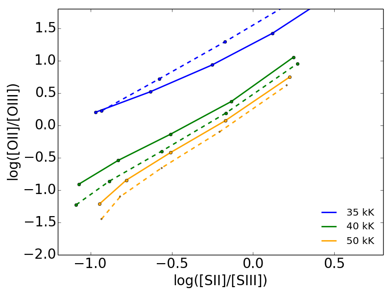
Figure 1: Relations between the emission-line ratios [S ii]/[S iii] and [O ii]/[O iii] predicted by some of the models described in the text. Each color represents different values of $T_{*}$. The values of log $U$ go from -3.5 to -1.5 in intervals of 0.5 dex from the lower left to the upper right part of the diagram. The solid lines join models with $Z$ = $Z_{\odot}$ while the dashed lines join models with $Z$ = $Z_{\odot}$/5.

2 Model and method description

The routine designed to calculate both $U$ and $T_{*}$ from the emission lines used in the definition of the $\eta\prime$ parameter is very similar to the Hii-Chi-mistry (Pérez-Montero, 2014) code used to derive chemical abundances in nebulae ionized by massive stars. The method consists of comparison between certain observed emission-line fluxes and the corresponding predictions made by a large grid of photoionization models covering the expected conditions in the studied object or position in an object.

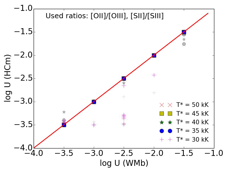
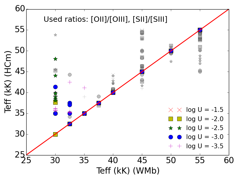
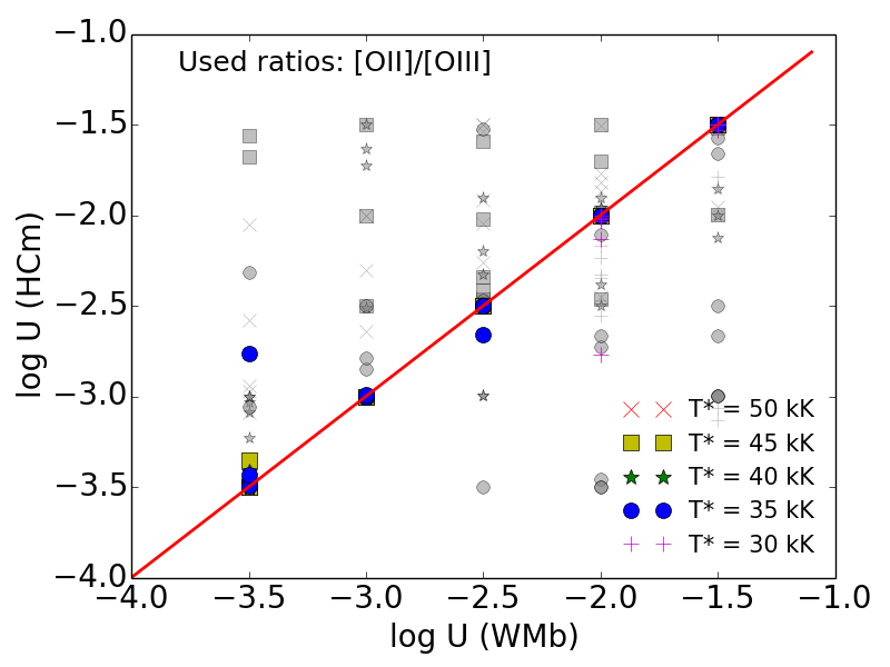
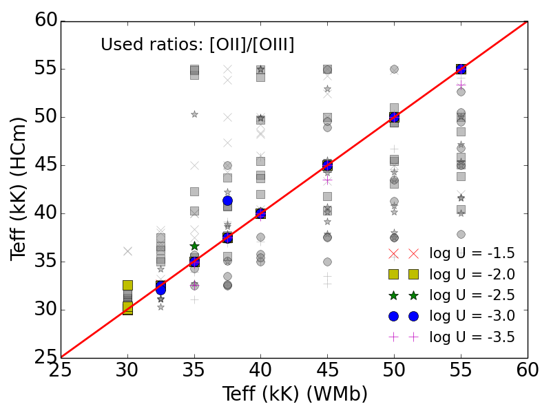
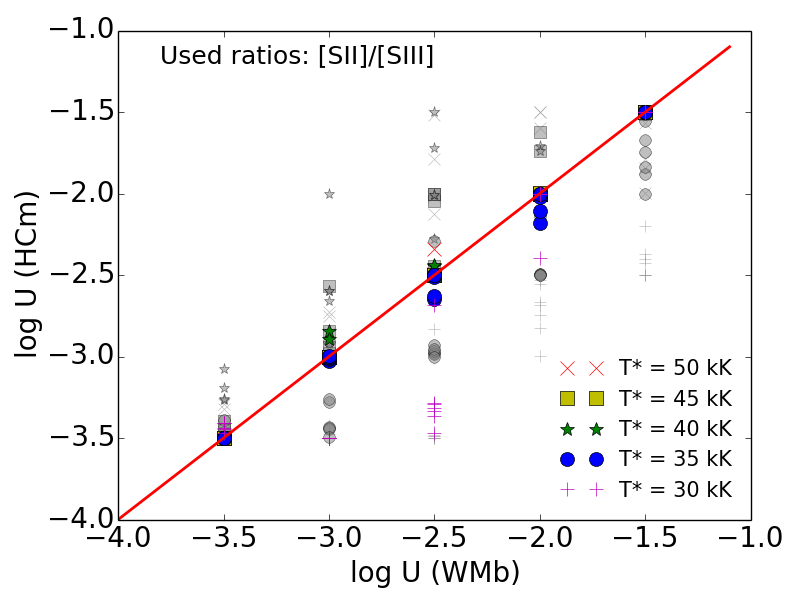
Figure 2: Comparison between the input $U$ (left-hand column) and $T_{*}$ (right-hand column) of the grid of models and the same properties predicted by our code using the corresponding different sets of emission-line ratios. In the top row the code uses as input both [O ii]/[O iii] and [S ii]/[S iii] line ratios. In the middle row we show the comparison when only the [O ii]/[O iii] emission-line ratio is used. Finally, in the bottom row we show the results when the code only makes use of the [S ii]/[S iii] emission-line ratio. In all panels thick coloured symbols correspond to calculations performed using metallicity as an input of the code, while thin-grey symbols leave metallicity as a free parameter.

The grid of models used in the routine described here was calculated using the code Cloudy v.17.00 (Ferland et al., 2017), which gives the relative intensities of the lines emitted by a one-dimensional distribution of gas ionized by a central source. For each model single ionizing source we used the SEDs of WM-Basic (Pauldrach et al., 2001) stellar atmospheres with $T_{*}$ values at 30, 32.5, 35, 37.5, 40, 45, 50, and 55 kK at the same $Z$ as the surrounding gas distribution. According to Zastrow et al. (2013) the synthetic WM-Basic SEDs in photoionization models lead to a better agreement with observed emission-line ratios in single-star H ii regions where they can be directly compared with the SED of the ionizing source.

For the gas we considered different $Z$ values scaled to the one of the oxygen abundance using the solar proportions given by Asplund et al. (2009) at the values 12+log(O/H) = 7.1, 7.4, 7.7, 8.0, 8.3, 8.6, and 8.9. We assumed in all models a constant electron density of 100 particles cm^-3 and a standard gas-to-dust mass ratio and depletion of the corresponding refractory elements. For $U$ we covered the values log $U$ = -3.5, -3.0, -2.5, -2.0, and -1.5. The stopping criterion to recover the calculated set of emission lines was reached when the electron temperature of the gas was lower than 4 000 K, which results in all models in a spherical geometry. The total number of models of the grid is then 280.

The python code Hii-Chi-mistry-Teff (hereafter HCm-Teff) makes a direct comparison between the model-predicted [O ii] 3727 Å relative to [O iii] 5007 Å and [S ii] 6717,6731 Å relative to [S iii] 9069 Å emission-line ratios with the corresponding reddening-corrected observed values in arbitrary units to give an estimation of both $U$ and T_∗. Although in the definition of the $\eta\prime$ parameter both lines of the [O iii] and [S iii] doublets are included, as there is a theoretical relation between the intensities of these lines [i.e. I(5007 Å) = 3$\times$ I(4959) and I(9069) = 2.44 $\times$I(9532 Å] that does not make it necessary to use of all them. In the case of [S iii] this is convenient as many times the emission line at 9532 Å is affected by atmospheric absorption, although this also depends on the redshift of the studied object. In addition it is necessary to be cautious with the extinction correction of these lines in the near-IR when it is performed in relation to H$\beta$ and it is convenient to use the close hydrogen recombination lines of the Paschen series to provide relative intensities that can be later expressed in terms of other lines in the optical range.

The code requires the oxygen abundance in each input observed object or position as the models predict a large dependence of the emission lines on $Z$. In Figure 1 we see the relation between both oxygen and sulphur optical emission-line ratios and the prediction from our grid of models for different $T_{*}$ at two $Z$ values ($Z_{\odot}$ and $Z_{\odot}/5$). As can be seen, the lines of equal $T_{*}$ tend to lie in a lower position for lower $Z$ and this effect is more noticeable for higher $T_{*}$. For this reason the code first interpolates a subset of emission-line predictions at the chosen oxygen abundance. In case this parameter is not provided the code assumes the complete grid of models in the calculation, which translates to a larger uncertainty of the final derived products.

Once the grid of models is chosen according to the provided $Z$, the code calculates both $U$ and $T_{*}$ as the weighted mean in the distribution of all the values in each model $i$ in the grid as

$$\log(U)_{f}=\frac{\sum_{i}\log(U)_{i}/\chi^{2}_{i}}{\sum_{i}1/\chi^{2}_{i}}$$ (3)

and

$$T_{*f}=\frac{\sum_{i}T_{*i}/\chi^{2}_{i}}{\sum_{i}1/\chi^{2}_{i}}$$ (4)

where the $\chi_{i}$ values in each model are calculated as the sum over the set of the normalized difference between certain observables, $O_{j}$, and the corresponding values predicted by each model, $T_{j}$, as

$$\chi_{i}^{2}=\sum_{j}\frac{(O_{j}-T_{ji})^{2}}{O_{j}}$$ (5)

The emission-line ratios used by the code as observed quantities are log ([O ii]/[O iii]) and log([S ii]/[S iii]) In case the four required lines are not available the code also allows us to perform the calculations using only one of the above emission-line ratios.

The errors are calculated as the standard deviations of these 1/$\chi^{2}$-weighted distributions. The code also requires the observed errors in each line, if available, and calculates their contribution to the corresponding $U$ and $T_{*}$ errors using a Monte Carlo iteration randomly varying the input intensities around the provided input errors. Then these two error sources are quadratically added by the code.

3 Comparison with models and observations

In order to test the validity of our method to estimate both $U$ and $T_{*}$ using the emission lines in the softness parameter we took the predicted emission lines in the same WM-Basic single-star models as input for our code and we checked whether we recovered the same input $U$ and $T_{*}$.

In Figure 2 we show a comparison between the conditions imposed in each model and the log $U$ and $T_{*}$ values derived from the HCm-Teff code using only the lines. We also checked how using metallicity as an input in the code impacts the accuracy of the results. We tested three different cases attending to the use of both oxygen and sulphur emission-line ratios or using only one of them.

As can be seen we recover values close to the conditions of the models for both $U$ and $T_{*}$ when we use the two emission-line ratios using the metallicity as an input. For log $U$ the mean offset is lower than 0.05 dex at all values with a mean standard deviation of the residuals of 0.2 dex while for $T_{*}$ for values larger than 35kK the mean offset and the standard deviation of the residuals are both lower than 500 K. When metallicity is not added as an input to the code, but it is left as a free parameter and the code has to explore the entire grid, both $T_{*}$ and $U$ become more uncertain. Anyway, for $T_{*}$ the standard deviation of the residuals is on average 2500 K and the mean offset is always lower than 5000 K. On the contrary, for $U$ the dependence on metallicity looks to be lower, as the mean offset is lower in all cases than 0.1 dex, although the uncertainty is higher for lower excitations.

When we use only one of the two involved emission-line ratios we clearly see that [O ii]/[O iii] is more appropriate for the calculation of $T_{*}$ while [S ii]/[S iii] gives reliable estimates of log $U$. The offsets and standard deviations between the model conditions and those derived by our code are very similar to those obtained using both emission-line ratios in these quantities. On the other hand [O ii]/[O iii] can lead to deviations larger than 1 dex for low values of log $U$ and [S ii]/[S iii] can overestimate $T_{*}$ on average more than 5 kK at values lower than 40Kk. This trend is even more pronounced when metallicity is not used as an input in the code and the derivation of T_∗ using only [O ii]/[O iii] and log $U$ from [S ii]/[S iii] is much worse than when we have the two emission-line ratios. Besides, the determination of $U$ using [O ii]/[O iii] has an uncertainty higher than 0.5 dex in all cases, and even larger than 1 dex for low excitation. In the case of [S ii]/[S iii], the uncertainty to derive $T_{*}$ is never lower than 5000 K.

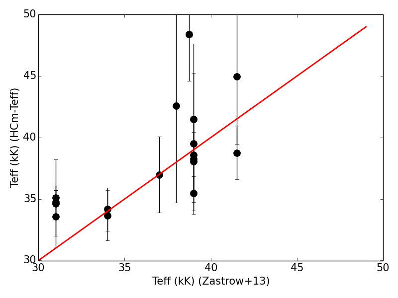
Figure 3: Comparison between the derived $T_{*}$ in single-star H ii regions given by Zastrow et al. (2013) and the results obtained from our code using only [O ii] and [O iii] emission lines, as provided by the authors.

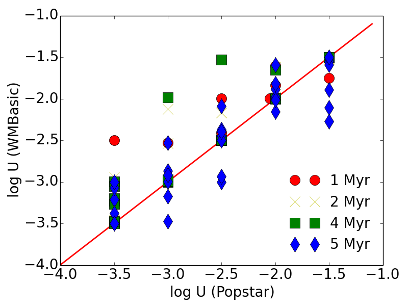
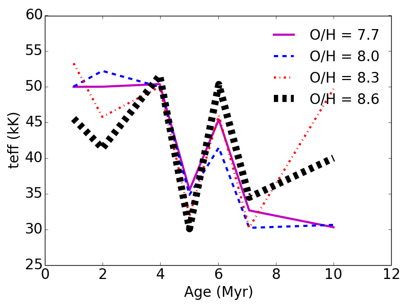
Figure 4: Results from the analysis of emission lines from models with popstar synthetic cluster SEDs using HCm-Teff. Left: comparison between the $U$ used as input in the models and the values predicted by the code for different ages. Right: relation between the age of the cluster and $T_{*}$ predicted by our code using the emission lines for different $Z$ values.

In addition it is possible to establish a direct comparison with data taking the spectroscopic optical observations of single-star H ii regions of the Galaxy given by Zastrow et al. (2013). These authors provide fittings from WM-Basic SED synthetic atmospheres and flux measurements of the most prominent emission lines in different long-sit positions in the surrounding gas, although the [S ii]/[S iii] emission-line ratio is not provided in this work. In Figure 3 we show the comparison between the $T_{*}$ values given by these authors and the values derived by our code using only [O ii] and [O iii], with the addition of $Z$ in those pointings with a measurement of the [O iii] auroral emission line at 4363 Å. As can be seen the scale of temperatures of the ionizing star is relatively well reproduced and the obtained values agree within the errors with the estimations given by the authors.

As a final test we checked the effect of applying our code using results from photoionization models based on single-star SEDS to the results from models using SEDs from massive clusters. To this aim we also produced a grid of photoionization models with the same gas conditions as described above but using a grid of POPSTAR (Mollá et al., 2009) with the same $Z$ as those defined in the grid of the code but with ages of 1,2,4,5, 7 and 10 Myr. We then used the resulting [O ii], [O iii], [S ii], and [S iii] predicted emission lines with their corresponding input $Z$ as input in our code.

In the left-hand panel of Figure 4 we show a comparison between the values of log $U$s chosen as input in the photoionization models calculated in this work using the popstar cluster synthetic SEDs and the results provided by HCm-Teff using the emission lines as input for the code. As can be seen the agreement is better for younger ages of the cluster. For an age of 1 Myr the mean offset of the log $U$ values is lower than 0.01 dex with a standard deviation of the residuals of only 0.1 dex. This dispersion grows with age and it is around 0.5 dex for ages larger than 5 Myr.

In the right-hand panel of the same figure we show a comparison between the resulting $T_{*}$ predicted by our code using only the emission lines and the corresponding cluster ages of the input models. As expected $T_{*}$ is higher for younger ages, with a decrease with age, a stage of hardening of the radiation corresponding to the Wolf-Rayet phase and a final decrease for old ages. The derived $T_{*}$ is lower at a specific age when $Z$ enhances as is expected from the effect of a larger blanketing from metals in the star atmospheres. Even for 12+log(O/H) = 8.6, the photoionization models do not predict the emission of high-excitation lines like [O iii] and [S iii] for ages larger than 6 Myr.

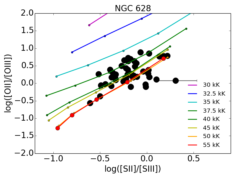
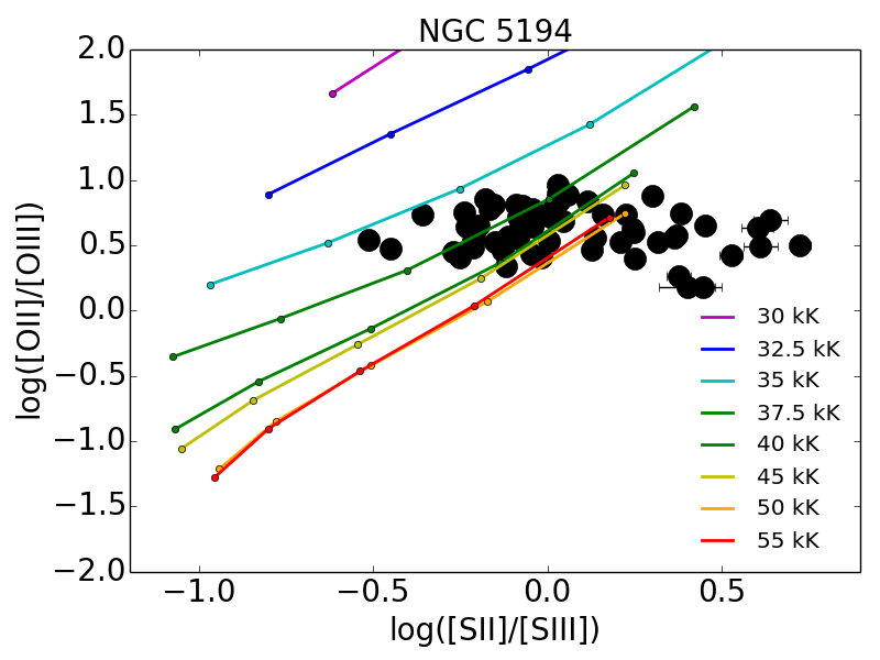
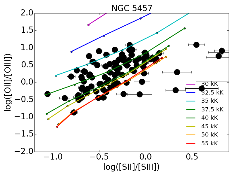
Figure 5: Relation between the emission-line ratios [S ii]6717,6731/[S iii]9069,9532 and [O ii]3727/[O iii]4959,5007 for the observed galaxies and comparison with models at different $T_{*}$ values at the average $Z$ measured in each galaxy.

4 Radial variations across galactic discs

4.1 Variations of the softness parameter

We evaluated the radial variations of the derived properties from our code HCm-Teff in the unique available sample in the literature that provides quality spectroscopic data for a representative subsample of H ii regions at all galactocentric distances, an accurate determination of the chemical abundances from the direct method, and with the required emission lines necessary for the calculation of the softness parameter (i.e. [O ii], [O iii], [S ii], [S iii]). This is the case of the chaos sample, which provides all this information for the galaxies NGC 628 (Berg et al., 2015), NGC 5194 (Croxall et al., 2015), and NGC 5457 (Croxall et al., 2016). We compiled from these works the listed reddening-corrected relative-to-H$\beta$ appropriate line fluxes and the derived total oxygen chemical abundances as derived from the direct method. In the case of the [S iii] 9069 Å line we rescaled its flux using the very close Pa10 line at 9015 Å to H$\beta$ using the expected theoretical ratio at a standard electron density and temperature to minimize reddening and flux calibration uncertainties. All the compiled H ii regions have H$\beta$ equivalent widths larger than 10 Å in emission, which ensures they are mostly ionized by very young episodes of star formation (Cid Fernandes et al., 2010) Overall, we compiled information from 46 H ii regions in NGC 628 [44 with a direct determination of 12+log(O/H)], 63 (29) in NGC 5194, and 102 (77) in NGC 5457.

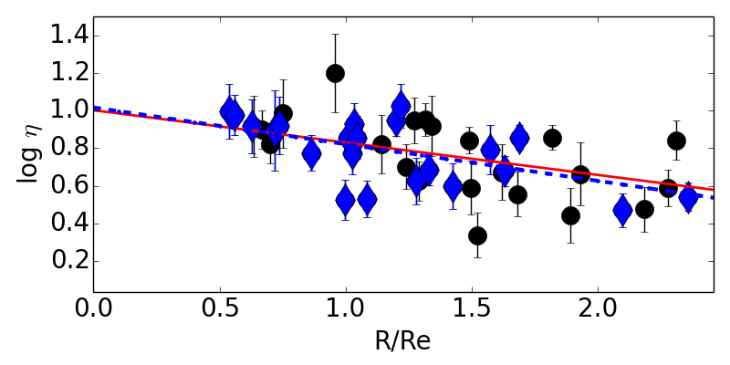
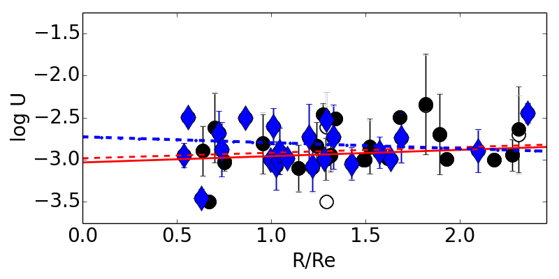
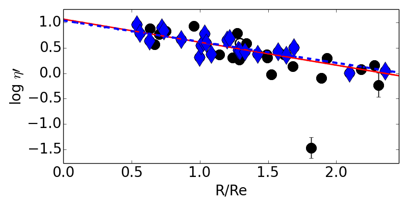
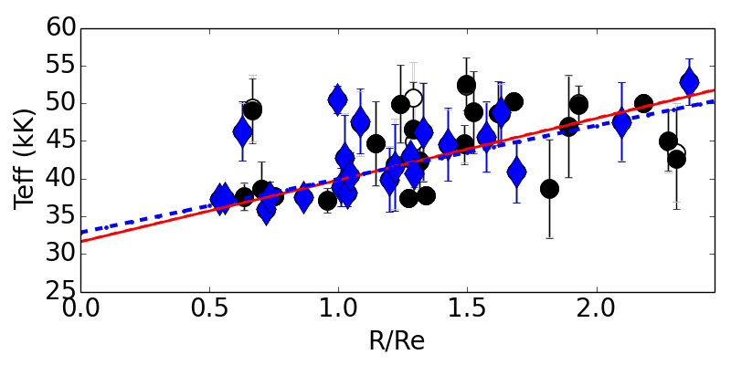
Figure 6: Radial distribution and linear fitting normalized to the effective radius for $\eta$ and $\eta\prime$ (left-hand panels), as derived from observations, and for $T_{*}$ and log U (right-hand panels) as derived using our code in NGC 628. The filled circles represent those H ii regions with a direct determination of the chemical abundance and its corresponding linear fitting is plotted with a dashed line. The white circles represent all the other regions whose O/H was derived using other methods. The linear fitting to the whole sample is represented with a solid line. Finally, blue diamonds represent those regions whose H$\alpha$ luminosity is larger than the average. The linear fitting to this subsample is represented with a blue dotted-dashed line.

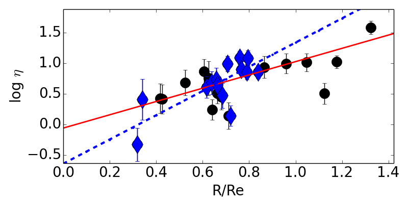
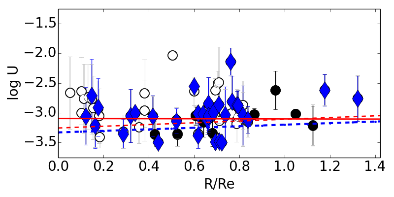
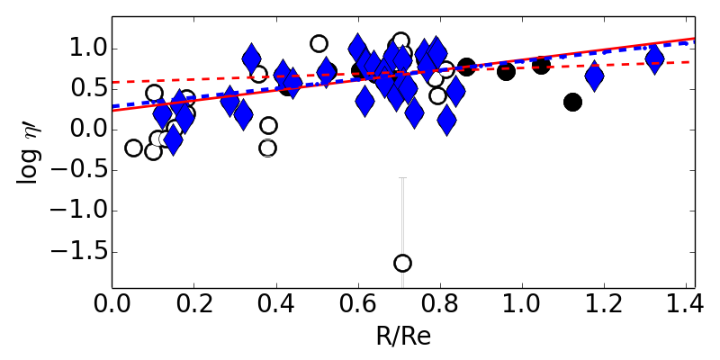
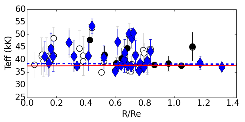
Figure 7: Same plots as those described in Fig.6 for the galaxy NGC 5194.

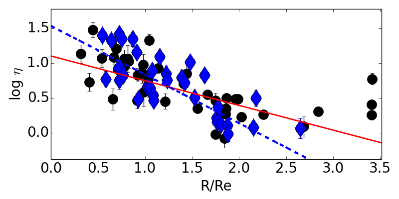
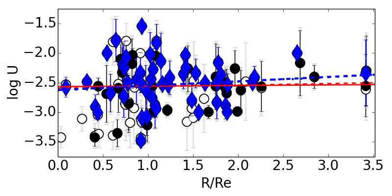
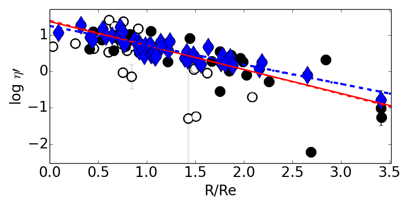
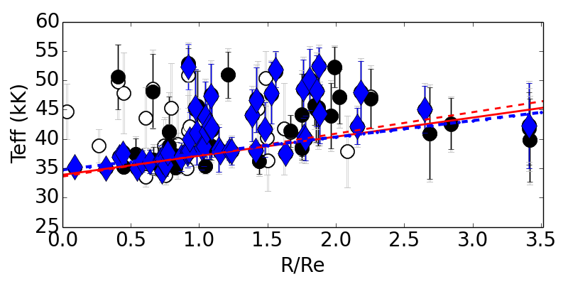
Figure 8: Same plots as those described in Fig.6 for galaxy NGC 5457.

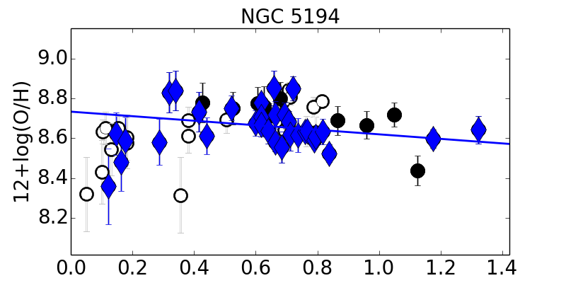
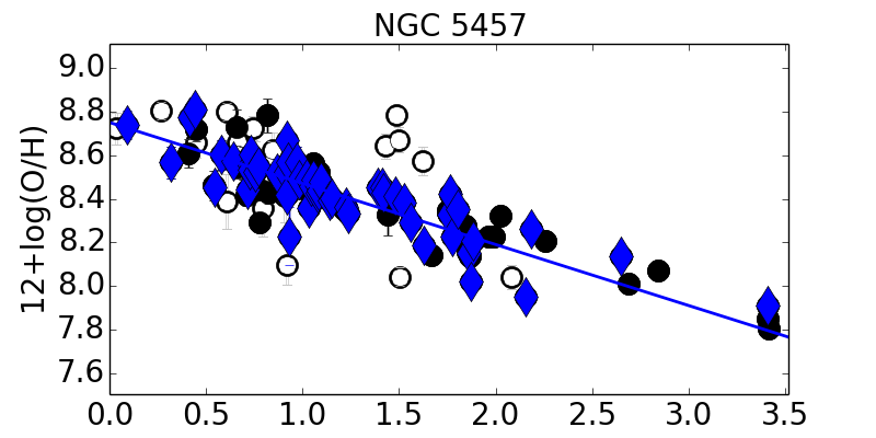
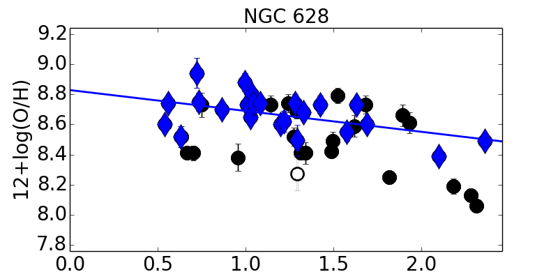
Figure 9: Radial distribution of the total oxygen abundances in the H ii regions of the three chaos galaxies. We show NGC 628 in the top panel, NGC 5194 in the middle panel, and NGC 5457 in the bottom panel. The radial scale is normalized to the effective radius in each object. The black circles represent regions whose abundances were derived using the direct method, the white circles have abundances derived using the HCM code, while diamonds represent regions with an H$\alpha$ luminosity larger than the average in each galaxy. The red solid line represents the error-weighted linear fitting to the whole sample. The dashed line represents the fitting to the regions with abundances derived following the DM, and the dot-dashed lines the fitting to the most luminous regions.

All these nearby star-forming disc galaxies present a spatial variation of $Z$ and, at the same time, different values of the hardening of the ionizing field of radiation in different positions of the galaxies as already described in Pérez-Montero & Vílchez (2009). In Figure 5 we show the position of the studied H ii regions of the three galaxies in the plane log([S ii]/[S iii]) vs log([O ii]/[O iii]). As reference we also plotted curves of equal $T_{*}$ from the models described above at the average $Z$ in each galaxy.

We can see that there is a good agreement between the position of the observations in the three galaxies and the space covered by the grid of models. Nevertheless there is a slight mismatch of some H ii regions lying below the space covered by the models that exceeds the maximum considered $T_{*}$. This partial disagreement between models and observations was already pointed out in Pérez-Montero & Vílchez (2009), notably for star-forming dwarf galaxies, and could be due to problems in the atomic coefficients used by the models, the stellar libraries, or to an oversimplification in the geometry of the models as the matter-bounded case is not assumed in the grid and this can largely affect the relative intensities of consecutive ionic stages across the radius of the ionized gas.

We explored the radial variation of the softness parameter in the three galaxies taking the corresponding deprojected galactocentric distance of each H ii region. We analysed both the $\eta$ parameter, based on ionic abundances only for those H ii regions with a direct estimation of the chemical abundance, and the $\eta\prime$ parameter, using only emission lines in all H ii regions. The results, normalized to the effective radius, are shown in Figure 6 for NGC 628, Figure 7 for NGC 5194, and Figure 8 for NGC 5457.

In Table LABEL:slopes we list the slopes of the corresponding linear fittings performed to the radial distribution of these parameters considering the weights of the associated errors as propagated from the reported relative intensities and ionic abundances. The fittings were calculated using the radii normalized to the effective radius in each object.

Both NGC 628 and NGC 5457 show very clear decreasing trends of $\eta^{\prime}$, while NGC 5194 presents an increasing radial variation, although sensibly flatter when we consider only those H ii regions with a direct determination of the oxygen abundance. These trends are confirmed when we explore the radial variations of $\eta$, which is possible in most of the H ii regions of the chaos sample due to the precision in the determination of the involved ionic abundances in each H ii region. The radial variations in these three objects were already observed by Pérez-Montero & Vílchez (2009) using a lower number of H ii regions.

We also checked whether these radial trends are affected by the luminosity of the regions, as $T_{*}$, one of the quantities governing the behavior of the softness parameter, could be affected by the statistical fluctuations in low-scale regions (Cerviño et al. 2000). We considered the mean H$\alpha$ luminosity of the H ii region distribution in each galaxy as a lower limit to look for differences with respect to the total sample. We found the values 10^39.8 erg/s in NGC 628, 10^40.1 erg/s in NGC 5194, and 10^40.1 erg/s in NGC 5457. Taking starburst99 (Leitherer et al., 1999) models as a reference, these luminosities would correspond to cluster masses of about 3$\times$10³ M_⊙ in NGC 628 and 6$\times$10³ M_⊙ in NGC 5194 and NGC 5457, assuming an instantaneous burst at $Z$ = $Z_{\odot}$ and standard conditions of the cluster. As can be seen in the corresponding figures and in Table LABEL:slopes the observed trends do not vary significantly even when we only consider the top half of the H$\alpha$ distribution of the H ii regions in these galaxies.

Nevertheless we still have to explore whether these radial variations of both softness parameters can be associated with a real radial variation of the hardening of the ionizing stellar radiation field across the galactic discs.

Table 1: Slopes and errors of the linear fittings for the studied galaxies normalized by the corresponding effective radius. We consider three different subsamples of regions in each galaxy: (i) the whole sample, (ii) only H ii regions with a direct determination of the chemical abundance, and (iii) regions with H$\alpha$ luminosity larger than the average in each galaxy.

Object	Selection	Regions	$\alpha$ (log $\eta$)	$\alpha$ (log $\eta\prime$)	$\alpha$ (log U)	$\alpha$ (T∗)	$\alpha$ (12+log(O/H))
	(DM)		(dex/Re)	(dex/Re)	(dex/R${}_{e})$	(kK/Re)	(dex/Re)
NGC 628	All	46	–	-0.45 $\pm$ 0.05	0.07 $\pm$ 0.10	8.2 $\pm$ 0.7	-0.21 $\pm$ 0.05
	O/H from DM	44	-0.17 $\pm$ 0.05	-0.45 $\pm$ 0.05	0.07 $\pm$ 0.09	8.2 $\pm$ 0.7	-0.21 $\pm$ 0.05
	L(H$\alpha$) $>$mean	23	-0.19 $\pm$ 0.06	-10.41 $\pm$ 0.07	-0.07 $\pm$ 0.15	7.1 $\pm$ 1.8	-0.14 $\pm$ 0.04
NGC 5194	All	68	–	0.62 $\pm$ 0.11	-0.01 $\pm$ 0.19	0.2 $\pm$ 1.8	0.01 $\pm$ 0.06
	O/H from DM	29	1.08 $\pm$ 0.21	0.18 $\pm$ 0.16	0.15 $\pm$ 0.28	-0.5 $\pm$ 2.6	-0.21 $\pm$ 0.08
	L(H$\alpha$) $>$mean	32	1.98 $\pm$ 0.63	0.55$\pm$ 0.15	0.13 $\pm$ 0.38	-0.1 $\pm$ 4.7	-0.11 $\pm$ 0.07
NGC 5457	All	102	–	-0.66 $\pm$ 0.05	0.01 $\pm$ 0.07	3.3 $\pm$ 0.5	-0.27 $\pm$ 0.02
	O/H from DM	78	-0.35 $\pm$ 0.05	-0.68 $\pm$ 0.05	0.03 $\pm$ 0.08	3.6 $\pm$ 0.6	-0.26 $\pm$ 0.02
	L(H$\alpha$) $>$mean	52	-0.70 $\pm$ 0.08	-0.53 $\pm$ 0.04	0.07 $\pm$ 0.09	2.8 $\pm$ 0.6	-0.28 $\pm$ 0.02

4.2 Radial variation of $U$ and $T_{*}$

In order to check whether the obtained radial variations of the softness parameter in the three studied galaxies can be really interpreted as a radial variation of the hardening of the ionizing stellar field of radiation, we applied HCm-Teff, described in Section 2, to the sample of H ii regions.

We considered the oxygen abundances derived following the direct method given by CHAOS to constrain the grid of models in those H ii regions where it was possible. For the rest of the H ii regions without a direct estimation of $Z$ we resorted to the code Hii-Chi-mistry v.3.0 (HCm; Pérez-Montero 2014) to provide an estimation of 12+log(O/H) for the calculation of both $U$ and $T_{*}$. This code follows a very similar methodology to the one described in this work as it is based on a Bayesian-like approach to establish a comparison between the measured optical emission lines to the values predicted by a large grid of photoionization models. The resulting abundances are consistent with the direct method even in the absence of any auroral line although the uncertainty in this case is larger. In addition the error fluxes of the used emission lines are taken into account by the code for the final error calculation following a Monte Carlo iteration. We checked that the oxygen total abundances derived using the HCm code in the absence of the [O iii] 4363 Å line agree with the abundances derived following the direct method in those chaos H ii regions with any auroral line with a dispersion lower than 0.2 dex and without any systematic offset even in the regime of oversolar metallicity. Although different authors point towards a systematic offset of around 0.2 dex between the abundances derived from the direct method and those coming from photoionization models (i.e. Blanc et al. 2015; Vale Asari et al. 2016), the Hii-Chi-mistry code obtains no discrepancies by means of an assumed empirical relation between metallicity and excitation. The agreement with the H ii regions of the chaos sample is also discussed in Pérez-Montero et al. 2016.

We calculated the slopes of the error-weighted linear fittings of log $\eta\prime$, 12+log(O/H), log $U$ and $T_{*}$ and we normalized to the effective radius (R_e) (i.e. the radius encompassing half of the total luminosity). The slopes of the linear fittings and their corresponding errors are listed in Table LABEL:slopes.

For the sake of consistency, we provide the results of the radial variations and fittings both for $U$ and $T_{*}$ and for those H ii regions only with a direct determination of O/H to explore whether the obtained dispersions can be caused due to the factor of including objects with abundances obtained from other methods. We also show in Figure 9 the radial profiles of the total oxygen abundance in the three galaxies, taking the whole analysed sample and only for regions with a direct estimation of the electron temperature. Clear negative radial variations of the metallicity are observed in the three objects, with slopes larger than -0.2 dex/R_e, in agreement with the results obtained by the chaos collaboration. Only in the case of NGC 5194 do we obtain a much flatter slope when the H ii regions in the central regions of this galaxy are considered using the values derived by HCM.

For the calculation of $T_{*}$ in those H ii regions that lie in the plane [S ii]/[S iii] vs. [O ii]/[O iii] below the space covered by the grid of models, we checked that the code always assigns to them values larger than 50k K, but we cannot confirm in these cases whether the position of these regions in the plot can be due to other factors (i.e. different geometry, photon leakage).

The distributions of the derived log $U$ and $T_{*}$ for H ii regions in the three galaxies across the deprojected galactocentric distances normalized to the effective radius are plotted in Figure 6 for NGC 628, Figure 7 for NGC 5491, and Figure 8 for NGC 5457.

Though the radial behavior of $\eta$ is different in the three galaxies, they show a flat radial slope of the ionization parameter so the H ii regions studied here present a similar ionization parameter, on average, independently of their galactocentric distance. We do not observe any great difference between the slopes fitted to all regions or just to the regions with a direct determination of the abundance or to the most luminous ones. The slope only appears to be slightly higher in NGC 5194 when only regions with a direct determination of O/H are considered. At the same time the H ii regions in the three galaxies present average excitation properties that are in agreement with their sizes and average $Z$, taking the characteristic value of the obtained linear fitting at the effective radius. In this way NGC 628 has a characteristic log $U$ value of -2.96, NGC 5194 has -3.11, and NGC 5457 has -2.56.

Regarding $T_{*}$ we observe radial variations consistent with those observed in the softness parameter, although the sign of the slope observed in $\eta$ cannot be always interpreted as radial variations of $T_{*}$ in a determined sense. On one hand the two galaxies with clear decreasing slopes of the $\eta$ parameter, NGC 628 and NGC 5457, present at the same time very clear increasing slopes of $T_{*}$. Therefore in these two galaxies the observed variation of the softness parameter can be directly associated with a hardening of the stellar radiation across the galactic disc. On the other hand, NGC 5194, presenting increasing slopes of $\eta$, has in average a flat radial distribution of the $T_{*}$ values. These flat radial distributions cannot be related to the large number of H ii regions not covered by the grid of models in this galaxy. Considering only the 35 H ii regions with values of [O ii]/[O iii] and [S ii]/[S iii] values reproduced by our grid, the slope of the linear fitting for $T_{*}$ is 500 $\pm$ 600 K/R_e, and for log $U$ it is -0.22 $\pm$ 0.26 dex/R_e.

Neither the obtained slopes nor the associated dispersions vary significantly when only H ii regions with a direct determination of the abundance or regions belonging to the top half of the H$\alpha$ luminosity distribution are considered in the three galaxies.

Therefore, though the direct analysis of the radial variation of the softness parameter in these three well-studied disc galaxies cannot be directly interpreted as equivalent radial variations of $U$ or $T_{*}$ we find some correlation between the obtained slopes. Moreover the results evidence the need for a detailed analysis of all involved quantities in the softness parameter instead of using this parameter as a direct indicator of the properties of an H ii region.

4.3 Correlation with other properties

Table 2: Slopes of the linear fittings to log $\eta\prime$ and 12+log(O/H) as measured, and log $U$ and $T_{*}$ as derived using our code as a function of the galactocentric distance in units of kpc for the chaos galaxies studied in this work and for the sample analyzed in Pérez-Montero & Vílchez (2009). We provide the references of the observed, used emission lines in each object.

Object	$\alpha$ (log $\eta\prime$)	$\alpha$ (O/H)	$\alpha$ (log $U$)	$\alpha$ ($T_{*}$)	Ref.
	dex/kpc	dex/kpc	dex/kpc	K/kpc
NGC 300	-0.059 $\pm$ 0.030	-0.008 $\pm$ 0.006	0.035 $\pm$ 0.029	1900 $\pm$ 800	Bresolin et al. (2009)
NGC 598	-0.175 $\pm$ 0.023	-0.016 $\pm$ 0.004	0.105 $\pm$ 0.039	1100 $\pm$ 300	Vilchez et al. (1988)
NGC 628	-0.062 $\pm$ 0.015	-0.029 $\pm$ 0.010	0.017 $\pm$ 0.023	1800 $\pm$ 200	Berg et al. (2015)
NGC 1232	-0.010 $\pm$ 0.018	-0.002 $\pm$ 0.029	0.052 $\pm$ 0.008	-100 $\pm$ 200	Bresolin et al. (2005)
NGC 1365	-0.010 $\pm$0.005	0.002 $\pm$ 0.005	-0.003 $\pm$ 0.007	-100 $\pm$ 100	Bresolin et al. (2005)
NGC 2403	-0.083 $\pm$0.022	-0.051 $\pm$ 0.028	-0.039 $\pm$ 0.031	2100 $\pm$ 300	Garnett et al. (1997)
NGC 2903	-0.003 $\pm$ 0.002	–	0.047 $\pm$ 0.040	500 $\pm$ 600	Bresolin et al. (2005)
NGC 2997	-0.002 $\pm$ 0.001	0.000 $\pm$ 0.001	0.030 $\pm$ 0.055	800 $\pm$ 600	Bresolin et al. (2005)
NGC 5194	-0.118 $\pm$ 0.116	-0.042 $\pm$ 0.025	0.063 $\pm$ 0.055	-300 $\pm$ 100	Bresolin et al. (2004)
NGC 5194	0.078 $\pm$ 0.012	0.003 $\pm$ 0.006	0.001 $\pm$ 0.002	0 $\pm$ 200	Croxall et al. (2015)
NGC 5236	-0.084 $\pm$ 0.046	-0.052 $\pm$ 0.028	0.012 $\pm$ 0.052	400 $\pm$ 500	Bresolin et al. (2005)
NGC 5457	-0.032 $\pm$ 0.009	-0.019 $\pm$ 0.005	0.002 $\pm$ 0.003	400 $\pm$ 100	Kennicutt et al. (2003)
NGC 5457	-0.077 $\pm$ 0.005	-0.030 $\pm$ 0.002	0.001 $\pm$ 0.007	400 $\pm$ 100	Croxall et al. (2016)

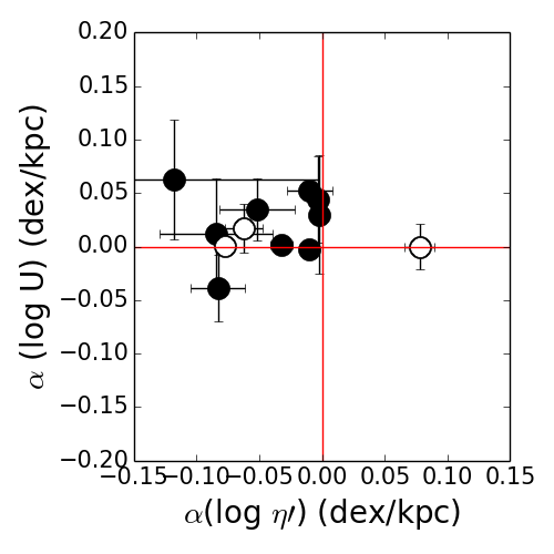
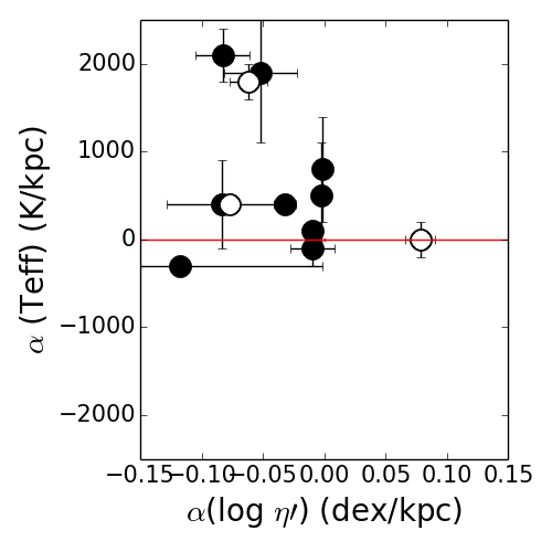
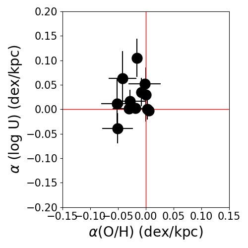
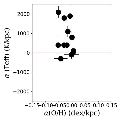
Figure 10: Relation between the slopes of the linear fittings and the radial distributions of several properties in the studied galaxies. The upper row represents the relation between the slopes of log $\eta\prime$ and log $U$ and T_∗ while in the lower row we show the slopes of 12+log(O/H) with the same derived properties. The white circles represent the chaos sample and the black circles the sample studied in Pérez-Montero & Vílchez (2009).

Once the different dependences of the softness parameter on the $U$ and $T_{*}$ have been analysed in the three studied objects, it is possible to re-examine the radial variations of these properties as a function of the slopes of other well-known derived quantities in the same galaxies and to establish correlations with other integrated properties.

In any case, the three-galaxy sample with good-quality data from the chaos collaboration is not enough to extract general conclusions about the behavior of these radial variations. In fact, only two out of the three galaxies present the decreasing gradient of the softness parameter already observed in the majority of the sample studied in Pérez-Montero & Vílchez (2009). Of the nine analysed galaxies with available data to study the radial variation of the softness parameter in Pérez-Montero & Vílchez (2009), most present a clear decreasing radial variation. For that reason, although that sample has a much lower number of H ii regions in each object and the determination of chemical abundances in each object is more uncertain, we reanalysed this sample in order to inspect the causes of the radial variation of the softness parameter.

In Table 2 we give the results of the application of the HCm-Teff code to those H ii regions presenting the lines involved in the calculation of the softness parameter. We also list the three CHAOS objects studied above multiplying the obtained slopes by the effective radius to give them in dex kpc^-1 as in the rest of the objects. We also list in the same table the slopes of the linear fittings in the same H ii regions corresponding to the radial distribution of log $\eta\prime$ and 12+log(O/H), as derived from the direct method in those H ii regions with at least an auroral emission line.

As can be seen, all of them present a positive or flat gradient of log $U$ with the exception of NGC 1365, which presents a value compatible with a flat slope, and NGC 2403, in this case with a large dispersion in the obtained slope. In the same way all galaxies present a clear positive slope in the gradient of $T_{*}$ or values compatible with a flat slope, but in none of them do we obtain clear evidence of a negative slope of $T_{*}$ across the galactic discs.

In Figure 10 we show a comparison between the slopes of the softness parameter, as calculated using log $\eta\prime$, and the slopes for both $U$ and $T_{*}$ to inspect which physical property has a larger weight. Although it is not possible to extract a clear correlation because of the shortage of the analysed sample, there is a large coincidence between the sign of the slope of $\eta\prime$ and log $U$ and $T_{*}$ for almost all the objects. The general picture is that of a galaxy with a positive gradient of the softness parameter, which translates from the models in a positive or flat gradient for $U$ and $T_{*}$ but with no clear evidence about which of them has a larger weight on the softness parameter.

Most of the disc galaxies present at the same time lower O/H values at larger galactocentric distances as studied by the authors presenting the spectroscopic studies of the corresponding H ii regions. This could be related to the existence of an excitation variation with distance or with a lower value of $T_{*}$ in the innermost regions, where the amount of metals is higher. To evaluate the existence of these correlations, we show in the lower panels of Figure 10 the relation between the slopes of the linear fittings (as a function of radius in kpc) of the total oxygen abundance and log $U$ and $T_{*}$. As in the case of $\eta$ there is a general concordance between the sign of the O/H slopes and those of excitation and hardening of the radiation but, on the other hand, it is not possible to extract the main source of correlation.

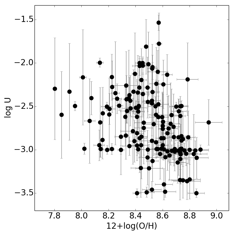
Figure 11: Relation between the total oxygen abundance as derived by the direct method and $U$ (left-hand panel) and $T_{*}$ (right-hand panel) derived from HCm-Teff in those H ii regions studied in the three chaos galaxies with the appropriate emission lines.

The existence of a correlation between $Z$ and $U$, in the sense that regions with a larger metal content are on average less excited, has been widely described and discussed in the literature (e.g. Pérez-Montero 2014) but it has been interpreted in terms of the additional dependence on $T_{*}$ of the emission-line ratios used to derive $U$. In fact, when we supply a methodology to resolve the dependence of emission lines on both $U$ and $T_{*}$ we appreciate a certain correlation between $Z$ and both the gas excitation and the hardness of the radiation. In Figure 11 we show the relation between the total oxygen abundance as derived by the direct method in the H ii regions of the three chaos galaxies and $U$ and $T_{*}$ as derived using the HCm-Teff code. We limit this plot to this sample as these H ii regions present a very accurate abundance determination from one or several auroral emission lines and were observed under much more homogeneous conditions. No clear general correlations are shown by the data in either plot; nonetheless, the influence of other HII region parameters (e.g. evolution of the ionizing clusters; geometry, multiple versus compact ionizing sources, luminosity/size) could be operating for each sample.

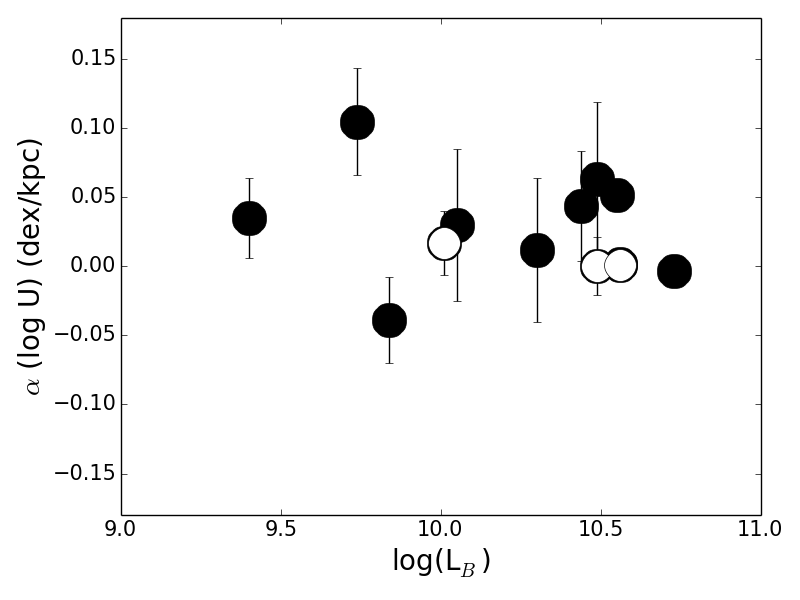
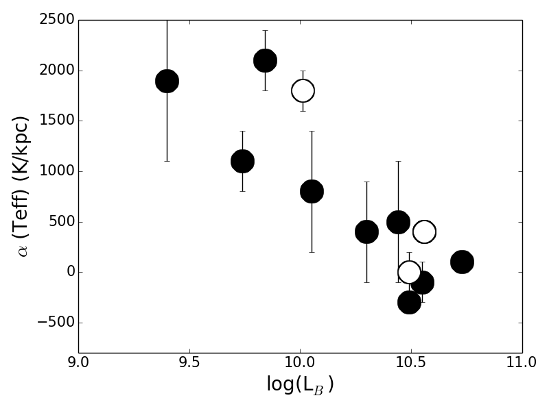
Figure 12: Relation between integrated luminosity in the $B$ band and the slopes of the linear fittings to log $U$ (left) and $T_{*}$ (right). The white circles correspond to the three chaos galaxies, while the black circles represent the results from the galaxies presented in Pérez-Montero & Vílchez (2009).

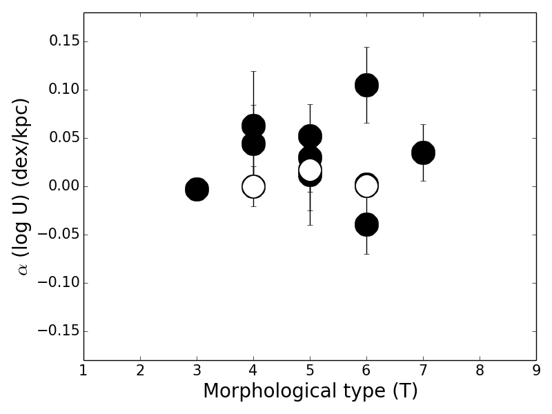
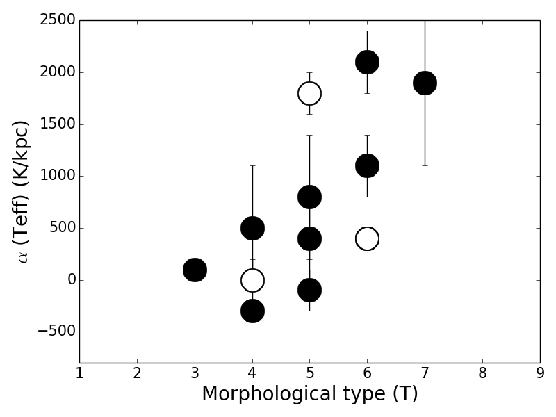
Figure 13: Relation between the Hubble morphological type and the slopes of the linear fittings to log $U$ (left) and $T_{*}$ (right). The white circles correspond to the three chaos galaxies, while the black circles represent the results from the galaxies presented in Pérez-Montero & Vílchez (2009).

Another interesting test to check the existence of a connection between excitation, radiation hardness, and $Z$ is exploration of the relation between the average radial variation of the softness parameter and the integrated luminosity of the galaxies. Pérez-Montero & Vílchez (2009) pointed out a certain correlation between the luminosity of galaxies and the slope of the linear fittings of log $\eta\prime$, as it has been observed in the case of $Z$. With the current study it is possible to figure out whether this correlation is mostly due to the dependence of the softness parameter on $U$ or on $T_{*}$. In Figure 12 we show this relation both for $U$ and for $T_{*}$ though no global trend can be extracted owing to the scarcity of our sample. Despite the large dispersion, it is possible to extract some average trends. In this way for those galaxies with log $L_{B}$ $<$ 10.2 erg/s the average log $U$ slope is 0.03 ($\pm$0.04) dex/kpc, while for galaxies with log $L_{B}$ $>$ 10.2 erg/s it is 0.02 ($\pm$ 0.02) dex/kpc, both values consistent to within the errors. However, a much clearer correlation is found when we perform the same analysis regarding $T_{*}$ as the slope for less bright galaxies (log $L_{B}$ $<$ 10.2 erg/s) is 1500 $\pm$ 400 K/kpc, while for the brighter galaxies (log $L_{B}$ $>$ 10.2 erg/s) is the mean value is only 400 $\pm$ 300K/kpc. This difference in the observed slopes appears well established; thus in order to derive a precise value a study with a larger number of galaxies will shed more light on the gradient of the hardening of the field of radiation in disc galaxies.

In the same way we explored the possible existence of a correlation between the slopes of these gradients and the Hubble morphological type. In Pérez-Montero & Vílchez (2009) it appeared that galaxies with a later type present on average more pronounced $\eta\prime$ slopes. In Figure 13 we now show this relation once the dependence of $\eta\prime$ has been divided in $U$ and $T_{*}$. As in the case of the total integrated luminosity the existence of a possible correlation appears now only in the case of the radial variation of the harness of the ionizing radiation. Galaxies with later Hubble types (T $>$ 5) have larger $\alpha_{T*}$ (1100 $\pm$ 500 K/kpc) than those with earlier types (T $\leq$ 5) which have on average 400 $\pm$ 500 K/kpc. On the contrary no noticeable difference is found for the case of the ionization parameter. This difference in the average slopes of $T_{*}$ as a function of the morphological type can just be the effect of a bias in the luminosities of the galaxies for different types. Indeed the mean total luminosity in the $B$ band for late types is lower (log $L_{B}$ = 10.0 erg/s) than for the early ones (10.4 erg/s).

Several works have found a clear correlation of stellar mass, stellar mass surface density, and luminosity with morphological types (González Delgado et al., 2015; García-Benito et al., 2017), in the sense that early-type galaxies on average are more massive, redder, and show larger absolute magnitudes.

5 Summary and conclusions

In this work we have presented a new methodology to derive $U$ and $T_{*}$ in H ii regions. These two parameters are key to understand many of the observed relations between the relative fluxes of their most prominent emission lines.

Our approach departs from the relation between the so-called softness parameter with both $U$ and $T_{*}$. In this case we explore the two-dimensional space of the plane [S ii]/[S iii] versus [O ii]/[O iii] emission-line ratios in the optical and near-infrared spectral range to figure out the combination of them that leads to the observed patterns in $\eta$. According to photoionization models there is a non-negligible dependence on $Z$ in this plane that must also be resolved. We used a Bayesian-like code called Hcm-Teff that compares the prediction of a large grid of photoionization models in this plane with the observed emission-line ratios. The code also allows us to use only a given pair of lines but as the slope of the curves with the same $U$ and $T_{*}$ is not 1, [O ii]/[O iii] leads only to good estimations of $T_{*}$ while [S ii]/[S iii] is more appropriate for log $U$.

Among the limitations that the used grid of models can present when its results are compared to observations we can identify the use of a central single-star ionizing spectral distribution, the spherical matter-bounded geometry of the surrounding gas, and the constancy of density or dust-to-gas ratios. A more sophisticated exploration of these quantities in the models can lead to different degeneracies on the predicted emission-line fluxes that can lead to variations in the final results. In addition the energies involved in the ionization potentials of the used ions are not high enough to identify and compare very high $T_{*}$ values in the ionizing stars or clusters. The higher ionization potential is that of S²⁺ so the resulting grid is not valid to find stars hotter than 50-55 kK and the precision of the code at this regime is then also affected.

However, we think that this routine largely improves the accuracy and consistency of other recipes based only on the use of emission-line fluxes in integrated ionized gaseous nebulae when the analysis of the SED of the ionizing source cannot be carried out and it can be used as a robust comparative tool when no evidence of a large deviation from the simplified model exposed here is observed.

On this basis, we studied a large well-characterized sample of H ii regions in the local Universe. The spectroscopic study carried out by the chaos collaboration has provided us with good-quality data at different galactocentric distances for the four used emission lines and with auroral lines in many of them, which also permits a precise determination of the gaseous ionic abundances. The radial variation of the softness parameter in the three studied galaxies is very different, as already observed by Pérez-Montero & Vílchez 2009. While in NGC 628 and NGC 5457 we observe a clear decrease of the softness parameter, in NGC 5194 the slope is positive.

Applying the HCm-Teff code, we conclude that these radial variations can be explained in terms of a real hardening of the incident ionizing radiation in NGC 628 and NGC 5457. On the contrary there is not any clear evidence of a radial variation of $T_{*}$ in NGC 5194 despite the radial decrease of $\eta$. In none of the three galaxies do we detect a large radial variation of $U$. No large differences in these results are found when we limit the sample of studied H ii regions to those with a direct determination of the chemical abundance or to the sample of the most luminous objects to limit the effects of stochastic fluctuations on the initial mass function. However, we cannot discard the influence of the radial variation of metallicity on the observed patterns of the softness parameter, as in NGC 5491, the unique object in this sample with a negative slope in $\eta$, the O/H slope is flat when the innermost H ii regions with no measurement of any auroral line are taken into account.

Using the data compiled by Pérez-Montero & Vílchez (2009) to obtain more results we observe a certain trend to find galaxies with negative slope of $\eta\prime$ in concordance with a negative gradient of $Z$ and a positive gradient of excitation and $T_{*}$ as obtained by our code, but no clear correlation is found for any of the studied slopes. The existence of a global correlation between excitation or $T_{*}$ and metallicity is observed in both cases, so the influence of these two physical properties on the global behavior of the softness parameter must be extracted.

On the other hand a certain trend of having steeper $T_{*}$ gradients is observed in less bright galaxies, which has been widely observed in the case of gradients of $Z$. On the contrary a large difference is not found in the case of excitation. Therefore, there is some evidence pointing towards a real hardening of the field of radiation in spiral discs as a consequence of the native metallicity gradient observed in many of these objects. In all cases, a more comprehensive study of a large sample of disc galaxies with good determinations of the involved emission lines necessary to break the $T_{*}$-$U$ degeneracy and accurate oxygen abundances are required to give a statistically significant answer.

References

- Asplund et al. (2009) Asplund M., Grevesse N., Sauval A. J., Scott P., 2009, ARA&A, 47, 481
- Berg et al. (2015) Berg D. A., Skillman E. D., Croxall K. V., Pogge R. W., Moustakas J., Johnson-Groh M., 2015, ApJ, 806, 16
- Blanc et al. (2015) Blanc G. A., Kewley L., Vogt F. P. A., Dopita M. A., 2015, ApJ, 798, 99
- Bresolin et al. (2004) Bresolin F., Garnett D. R., Kennicutt Jr. R. C., 2004, ApJ, 615, 228
- Bresolin et al. (2005) Bresolin F., Schaerer D., González Delgado R. M., Stasińska G., 2005, A&A, 441, 981
- Bresolin et al. (2009) Bresolin F., Gieren W., Kudritzki R.-P., Pietrzyński G., Urbaneja M. A., Carraro G., 2009, ApJ, 700, 309
- Cerviño et al. (2000) Cerviño M., Luridiana V., Castander F. J., 2000, A&A, 360, L5
- Cid Fernandes et al. (2010) Cid Fernandes R., Stasińska G., Schlickmann M. S., Mateus A., Vale Asari N., Schoenell W., Sodré L., 2010, MNRAS, 403, 1036
- Croxall et al. (2015) Croxall K. V., Pogge R. W., Berg D. A., Skillman E. D., Moustakas J., 2015, ApJ, 808, 42
- Croxall et al. (2016) Croxall K. V., Pogge R. W., Berg D. A., Skillman E. D., Moustakas J., 2016, ApJ, 830, 4
- Diaz (1989) Diaz A. I., 1989, in Beckman J. E., Pagel B. E. J., eds, Evolutionary Phenomena in Galaxies. pp 377–397
- Díaz (1998) Díaz Á. I., 1998, Ap&SS, 263, 143
- Dors & Copetti (2003) Dors Jr. O. L., Copetti M. V. F., 2003, A&A, 404, 969
- Dors & Copetti (2005) Dors Jr. O. L., Copetti M. V. F., 2005, A&A, 437, 837
- Dors et al. (2017) Dors O. L., Hägele G. F., Cardaci M. V., Krabbe A. C., 2017, MNRAS, 466, 726
- Ferland et al. (2017) Ferland G. J., et al., 2017, Rev. Mex. Astron. Astrofis., 53, 385
- Fernández-Martín et al. (2017) Fernández-Martín A., Pérez-Montero E., Vílchez J. M., Mampaso A., 2017, A&A, 597, A84
- Fierro et al. (1986) Fierro J., Torres-Peimbert S., Peimbert M., 1986, PASP, 98, 1032
- García-Benito et al. (2017) García-Benito R., et al., 2017, A&A, 608, A27
- Garnett et al. (1997) Garnett D. R., Shields G. A., Skillman E. D., Sagan S. P., Dufour R. J., 1997, ApJ, 489, 63
- González Delgado et al. (2015) González Delgado R. M., et al., 2015, A&A, 581, A103
- Kennicutt et al. (2003) Kennicutt Jr. R. C., Bresolin F., Garnett D. R., 2003, ApJ, 591, 801
- Leitherer et al. (1999) Leitherer C., et al., 1999, ApJS, 123, 3
- McCall et al. (1985) McCall M. L., Rybski P. M., Shields G. A., 1985, ApJS, 57, 1
- Mollá et al. (2009) Mollá M., García-Vargas M. L., Bressan A., 2009, MNRAS, 398, 451
- Morisset (2004) Morisset C., 2004, ApJ, 601, 858
- Oey et al. (2000) Oey M. S., Dopita M. A., Shields J. C., Smith R. C., 2000, ApJS, 128, 511
- Pauldrach et al. (2001) Pauldrach A. W. A., Hoffmann T. L., Lennon M., 2001, A&A, 375, 161
- Pérez-Montero (2014) Pérez-Montero E., 2014, MNRAS, 441, 2663