Nondipole effects in atomic dynamic interference

Abstract

Nondipole effects in the atomic dynamic interference are investigated by numerically solving the time-dependent Schrödinger equation (TDSE) of hydrogen. It is found that the inclusion of nondipole corrections in the TDSE can induce momentum shifts of photoelectrons in the opposite direction of the laser propagation. The magnitude of the momentum shift is roughly proportional to the laser peak intensity and to the momentum component of the photoelectron along the laser propagation. By including the nondipole corrections of the Volkov phase into a semi-analytical model previously developed under the dipole approximation, all the main features of the momentum shifts can be nicely reproduced. Through an analytic expression, the origin of such momentum shifts is attributed to the nondipole phase difference between the two electron wave packets ejected in the rising edge and the falling edge, which will interfere with each other and result in the final fringe pattern. One important consequence of such momentum shifts is that they can smooth out the peak splitting induced by the dynamic interference in the photoelectron energy spectrum. Nevertheless, it should be emphasized that the dynamic interference persists in the photoelectron momentum distributions and is not suppressed at all for the laser parameters considered in this work.

I INTRODUCTION

Interference processes are at the heart of the optical and quantum mechanical phenomena, which can be realized through a spatial or temporal double-slit prototype. The availability of different new light sources has enabled the possibility to observe new types of quantum interference in atomic and molecular systems. For example, free-electron lasers (FELs) Emma et al. (2010); McNeil and Thompson (2010); Ishikawa et al. (2012) can now provide x-rays at wavelengths down to  1 Ångstrom with an unprecedented intensity around $10^{20}$ W/cm²) (see, e.g, a recent review in Ref. Young et al. (2018) and reference therein). For laser pulses at large photon energies and high intensities, the so-called “dynamic interference” in the atomic ionization has been theoretically observed Toyota et al. (2007, 2008); Demekhin and Cederbaum (2012a, b); Yu et al. (2013); Toyota et al. (2015); Toyota (2016); Artemyev et al. (2016); Baghery et al. (2017); Ning et al. (2018). It refers to the interference between two electronic wave packets respectively ejected in the rising and the falling edge of a laser pulse.

According to the Einstein’s photoelectric law, a single peak at $E=\omega-I_{p}$ is expected in the photoelectron energy spectrum for one-photon ionization at a low laser intensity. However, the single peak can gradually evolve into a multi-peak structure due to the dynamic interference when the laser intensity is increased. The conditions to observe such a dynamic interference are recently discussed Baghery et al. (2017); Jiang and Burgdörfer (2018). In fact, to observe the dynamic interference in the ground state of hydrogen at a moderately high laser frequency ($\sim$50 eV), the peak intensity needs to be high enough (above $10^{18}$ W/cm²) for the atomic stabilization to occur Jiang and Burgdörfer (2018). The relative theoretical studies are presently limited to the dipole approximation for the laser-atom interaction. However, one expects that the nondipole correction may play a non-negligible role at large photon energies with such a high laser intensity Reiss (2014); Førre and Simonsen (2014). For instance, the inclusion of the nondipole corrections may weaken the atomic stabilization Kylstra et al. (2000); Gavrila (2002); Popov et al. (2003); Førre et al. (2005); Emelin and Ryabikin (2014); Simonsen and Førre (2015); Staudt and Keitel (2003, 2006); Emelin et al. (2017).

In the dipole approximation, the time-dependent Hamiltonian is cylindrically symmetric for a linearly polarized laser pulse. However, the inclusion of the leading-order corrections of the nondipole effects will break the cylindrical symmetry of the Hamiltonian. As a result, the cylindrical symmetry of the angular distribution of the photoelectrons can also be broken when the nondipole corrections become non-negligible. In some cases, the asymmetrical angular distribution of the photoelectrons can be treated as a result of the interference between the dipole ionization paths and the nondipole ionization paths. Actually, there is a long history in calculating and measuring the asymmetrical distribution parameters Krässig et al. (1995); Martin et al. (1998); Dolmatov and Manson (1999); Derevianko et al. (2000); Hemmers et al. (2001); Krässig et al. (2002); Hemmers et al. (2003, 2006). Recently, several theoretical studies discussed the nondipole asymmetrical angular distributions Førre et al. (2006); Førre (2006); Zhou and Chu (2013); Førre et al. (2007); Moe and Førre (2018); Førre and Simonsen (2014). A related topic is the photon-momentum transfer and partition in the atomic and molecular ionization Smeenk et al. (2011); Titi and Drake (2012); Klaiber et al. (2013); Reiss (2013); Liu et al. (2013); Yakaboylu et al. (2013); Ludwig et al. (2014); Chelkowski et al. (2014, 2015); Ivanov (2015); Cricchio et al. (2015); Tao et al. (2017); He et al. (2017); Chelkowski et al. (2017); Wang et al. (2017); Lao et al. (2016); Chelkowski and Bandrauk (2018). Here, the momentum of the photon can be related to the average value of the photoelectron momentum along the laser propagation direction, whose nonzero value is an appearance of the broken cylindrical symmetry.

In this work, we particularly investigate the nondipole effects in the dynamic interference by numerically solving the time-dependent Schrödinger equation (TDSE). We present detailed angularly distinguished momentum spectra of the photoelectron within/byeond the dipole application. In the dipole approximation, the ring structures resulted from the dynamic interference in the momentum spectra are concentric at a zero momentum and symmetric about the line of the laser polarization according to the dipole transition. For the nondipole calculations, ring-like structures caused by the dynamics interference are still clearly present, but their geometric centers are apparently shifted in the opposite direction of the laser propagation and the rings are asymmetric about the axis of the laser polarization, which is due to the leading-order consideration of the magnetic force of the pulse. Such a shift in the momentum spectra can significantly suppress the peak splitting in the angularly integrated energy spectrum. We further explore the origin of the momentum shift and find that it is closely related to the nondipole phase differences between electrons emitted in the rising and falling edge of the laser pulse. By including the nondipole phase term into a semi-analytical model previously developed, the momentum shifts of the interference rings can be nicely reproduced.

II Methods

In the nonrelativistic situation, the dynamics of a hydrogen atom interacting with a classical electromagnetic field can be described by the time-dependent Schrödinger equation (atomic units are employed throughout unless otherwise stated),

$${i}\frac{\partial}{\partial t}\Psi(\mathbf{r},t)={H}\Psi(\mathbf{r},t),$$ (1)

where the full Hamiltonian in the velocity gauge is given by

$$H=\frac{1}{2}\left[\mathbf{p}+\mathbf{A}(\mathbf{r},t)\right]^{2}+V(\mathbf{r}).$$ (2)

With the consideration of the lowest-order nondipole correction Walser et al. (2000); Kylstra et al. (2001); Førre and Simonsen (2014); Cricchio et al. (2015), the time- and space-dependent vector potential $\mathbf{A}(\mathbf{r},t)$ for a laser pulse linearly polarized along the $z$ axis with a propagation direction in the positive $x$ axis can be written as

$$A_{z}(x,t)=A_{z}(t)+\frac{x}{c}E_{z}(t),$$ (3)

in which $A_{z}(t)$ is the vector potential usually adopted in the dipole approximation and $E_{z}(t)$ is the corresponding electric field, with $c$ being the vacuum light speed. Inserting Eq. (3) into Eq. (2), one obtains the leading-order corrected nondipole Hamiltonian,

$$H_{\mathrm{nondipole}} = -\frac{1}{2}\nabla^{2}+V(r)-iA_{z}(t){\partial}_{z}$$

$$-i\frac{x}{c}E_{z}(t){\partial}_{z}+\frac{x}{c}A_{z}(t)E_{z}(t),$$

in which we assume a hydrogen system, with a spherically symmetric potential $V(\mathbf{r})=V(r)=-1/r$.

To solve the TDSE, we expand the wave function in terms of the spherical harmonics for the angular coordinates. The resultant Schrödinger equation for the radial wave function can be solved using various discretization methods Peng and Starace (2006); Peng et al. (2015); Jiang and Tian (2017). In the present work, we use the finite difference for the radial coordinate $r$ and the split-operator technique for the short-time propagator Bauer and Koval (2006). The initial state is obtained by an imaginary time propagation in the absence of the external field until the ground-state energy is fully converged. And the final wave function ${\Psi}_{{f}}$ after the end of the external fields is projected onto the scattering states ${\Psi}_{\mathbf{p}}^{(-)}$ Starace (1982) to obtain the differential distribution of the photoelectron with a momentum $\mathbf{p}$, i.e.,

$$D(\mathbf{p})=D(p,\theta,\phi)=|\langle{\Psi}_{\mathbf{p}}^{(-)}|{\Psi}_{f}\rangle|^{2},$$ (4)

where $\theta$ is the angle between the photoelectron emission direction and the $z$-axis. To obtain the angularly integrated energy spectrum $D(E)$, one can change from the momentum to the energy space according to their Jacobian matrix and carry out the following integration,

$$D(E)=\int\!\!\int D(\mathbf{p}){|\mathbf{p}|}\sin{\theta}d\theta d\phi.$$ (5)

III Results and Discussions

In this section, we will present our main results, which are calculated for a linearly polarized Gaussian-shaped pulse with a carrier frequency of $\omega=53.6$ eV and with a full width at half maximum (FWHM) about 7 cycle. We will first examine the photoelectron energy distribution $D(E)$ at various laser intensities, where the dynamic interference gradually appears and drastic differences are observed between the dipole and the nondipole results at higher intensities. One may suspect that the dynamic interference is severely suppressed by the nondipole effects.

However, as one turns to compare the differential momentum distributions at the highest intensity used ($1\times 10^{19}~{}\mathrm{W/{cm}^{2}}$), one finds that nice interference still persists but with momentum shifts of the ring structures in the opposite direction of the laser propagation. Finally, by including the nondipole phase shift into our previous semi-analytical model based on the dipole approximation, we can reproduce the momentum shifts and find that they smooth out the dynamic interference in the angularly integrated spectrum $D(E)$.

For all the results presented in the following, full convergences are guaranteed against the change of the temporal and spatial parameters. Typically, the angular momentum $l$ is taken up to 40 and the maximum radial coordinate $r_{\mathrm{max}}\approx 2800$ a.u.

III.1 Nondipole effects in the energy spectrum

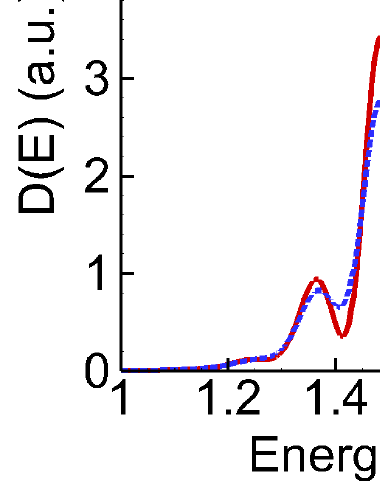
Figure 1: (Color online) The photoelectron energy distribution $D(E)$ for the 1s hydrogen state exposed to linearly polarized Gaussian-shaped pulses with a carrier frequency of $\omega=53.6$ eV and FWHM of 7 cycle at four different laser intensities: (a) $I_{0}=1.0\times 10^{17}~{}\mathrm{W/{cm}^{2}}$, (b) $I_{0}=1.0\times 10^{18}~{}\mathrm{W/{cm}^{2}}$, (c) $I_{0}=4.0\times 10^{18}~{}\mathrm{W/{cm}^{2}}$, and (d) $I_{0}=1.0\times 10^{19}~{}\mathrm{W/{cm}^{2}}$. Red solid line: the dipole result; blue dotted line: the nondipole result.

Previous studies on the dynamic interference were mainly focused on analysing the photoelectron energy spectrum. We show our results of photoelectron energy spectra in Fig. 1 at four different laser intensities. The results from the dipole approximation are consistent with previous studies, i.e., the dynamic interference does appear for pulse intensity above $10^{18}~{}\mathrm{W/{cm}^{2}}$ even for the ground state of hydrogen, due to the onset of the atomic stabilization Jiang and Burgdörfer (2018). Atomic stabilization can be involved if the laser intensity is larger than $c{\omega}^{4}/8\pi$ for the atomic hydrogen Jiang and Burgdörfer (2018). In addition, we notice that the results from the nondipole calculation can perfectly agree with those from the dipole calculations for laser intensity below $10^{18}$ W/cm², see Figs. 1(a) and 1(b). However, obvious differences can be observed for higher laser intensities, see Figs. 1(c) and 1(d). For present photon energy ($\sim 50$ eV), when the laser intensity is in the order of $10^{19}$ W/cm², one is approaching the limit of the dipole approximation (see, e.g. Fig.4 in Ref. Reiss (2014)) and the nondipole effects may be non-negligible. One can see from these results that the inclusion of the nondipole corrections can significantly suppress the peak splitting in the energy spectrum. Nevertheless, one can not draw the conclusion that the nondipole effects reduce the dynamic interference, as we will show below.

III.2 Momentum shifts in the rings of the dynamic interference

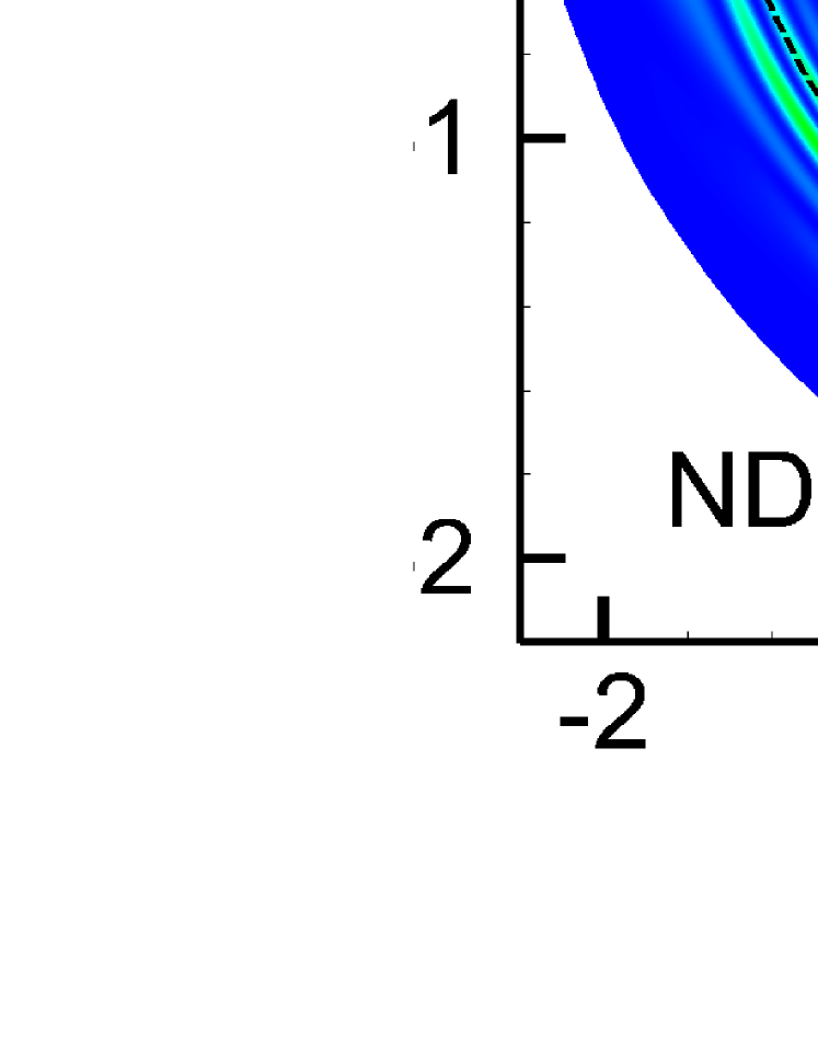
Figure 2: (Color online) The photoelectron momentum distribution $D(\mathbf{p})$ in the $p_{x}$-$p_{z}$ plane ($p_{y}=0$) plane at $I_{0}=1.0\times 10^{19}~{}\mathrm{W/{cm}^{2}}$. The upper (lower) half plane is the dipole (nondipole) result with a black solid (dashed) semi-circle as a reference to highlight the momentum shift.

In order to check whether the dynamic interference is destroyed by the nondiple effects, we turn to examine the differential distributions of photoelectrons in the momentum plane of $p_{x}$-$p_{z}$. In Fig. 2, we compare such momentum distributions from the dipole (upper half-plane) and nondipole (lower half-plane) calculations at the intensity of $1\times 10^{19}~{}\mathrm{W/{cm}^{2}}$.

Quite different from the gradual disappearance of the interference oscillations in the energy spectra of Figs. 1(c) and 1(d), one can see from Fig. 2 that the dynamic interference patterns are still present in the momentum space under the same laser parameters. As mentioned earlier, the inclusion of the nondipole terms in the Hamiltonian will break the cylindrical symmetry in the photoelectron distributions. Indeed, a careful examination for the lower half-plane can distinguish an asymmetric angular distribution in the positive and negative direction of the laser propagation, i.e., the spectrum is no more symmetric about the line of the laser polarization $z$-axis. The ring structures in the upper half plane of Fig. 2 precisely concenter at zero (marked as the origin point O), while the centers of those ring structures in the nondipole result in the lower half-plane of Fig. 2 are roughly shifted towards the opposite direction of the laser propagation (marked as the origin point O^′).

Such momentum shifts explain why the peak splitting in the angle-integrated energy spectrum is gradually smoothed out. From the TDSE calculations, we can extract the value of the center move from the point O to O^′ as the momentum shift $\Delta p$ at different laser intensities, which are shown by red solid circles in Fig. 3(a). One can see that the higher the laser intensity is, the larger the momentum shift is. The negative sign of $\Delta p$ means that the interference rings in the momentum space shift in the opposite direction of the laser propagation.

One expects, without considering the momentum shifts, the dynamic interference would still be present in the energy spectrum. To show this, in Fig. 3(b), we artificially move the shifted center O^′ of the nondipole interference patterns back to zero and recalculate the angle-integrated energy spectrum $D(E)$. Indeed, we find that the disappeared interference oscillations in Fig. 1(d) can be largely retrieved and the adjusted nondipole results agree with the dipole results rather well. From this respect, we can deduce that the dynamic interference process is not prohibited by the magnetic force for present laser parameters and the main nondipole effects should be the momentum shift of the interference patterns, whose underlying mechanism will be discussed in the following subsection.

III.3 Analytic expressions for the momentum shift

To see more clearly the nondipole effects, it’s better to examine the momentum distributions in the polar coordinates of the $p_{x}$-$p_{z}$ plane ($p_{y}=0$). As is shown in Fig. 4(a), the dipole results are identical for the electrons with $p_{x}>0$ and $p_{x}<0$. However, the angular distributions are drastically different for electrons with $p_{x}>0$ and those with $p_{x}<0$, as is respectively shown in Figs. 4(b) and 4(c): the momentum is shifted toward a smaller or a larger value. In the following, we will derive an analytical expression for the momentum shift.

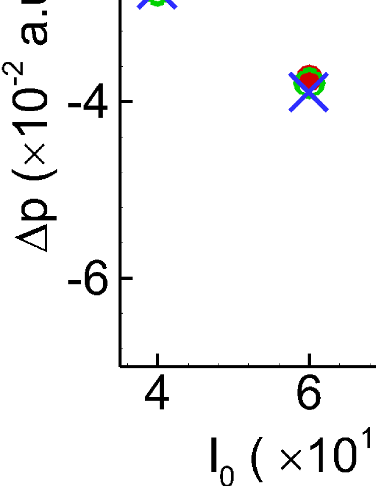
Figure 3: (Color online) (a) The momentum shift $\Delta p$ at various laser intensities: results in red solid circles (green open circles) are values extracted from the momentum distributions calculated by the nondipole TDSE (the semi-analytical model); the blue crosses refer to the analytic results from Eq. (13). In (b), angle-integrated energy spectra $D(E)$ are shown: for the dipole result as a red dotted line, and for the nondipole result respectively calculated before/after moving the center O^′ back to zero by a blue dashed/green solid line.

The dynamic interference origins from the AC-Stark shift of the initial ground state and the final continuum state. Models based on the dipole approximation can nicely explain the multi-peak structures in the energy spectrum Demekhin and Cederbaum (2012a); Jiang and Burgdörfer (2018). In the following, we are able to provide a physical explanation for the momentum shifts by including the nondipole corrections into our previous semi-analytical model Jiang and Burgdörfer (2018) and presenting an analytic expression for the momentum shift.

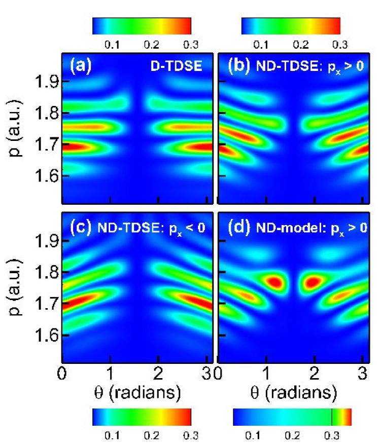
Figure 4: (Color online) The 2D photoelectron momentum distributions $D(\mathbf{p})$ in the $p_{x}$-$p_{z}$ plane ($p_{y}=0$) at $I_{0}=1.0\times 10^{19}~{}\mathrm{W/{cm}^{2}}$ are shown for: (a) the dipole TDSE calculation, (b) the nondipole TDSE calculation for $p_{x}>0$, (c) the nondipole TDSE calculation for $p_{x}<0$, and (d) semi-analytical model results for $p_{x}>0$.

It is too complicated to obtain an accurate expression for the AC-stark shift of the continuum state, but it is not difficult to get an analytic expression by neglecting the Coulomb potential in the Hamiltonian. The solution of the TDSE without considering the Coulomb potential is referred to the Volkov state. A Volkov state is a reasonable approximation for the continuum state when the laser intensity is high enough, as those considered in the present work. In addition, since the nondipole terms are only a small correction to the dipole interacting Hamiltonian, one expects that the magnitude of the transition matrix from the ground to the continuum state will not change much. On the contrary, for the dynamic interference discussed in this work, the phase of the transition matrix will play a much more important role. Therefore, let us satisfy ourselves by only including the nondipole modification in the phase.

The Volkov phase in the velocity gauge can be expressed as Joachain et al. (2011); He et al. (2017)

$$\Phi(t)=\phi_{0}(t)+\phi_{1}(t),$$ (6)

where

$$\phi_{0}(t)=\int_{-\infty}^{t}\left[\frac{p^{2}}{2}+p_{z}A(\tau)\right]d\tau$$ (7)

is the dipole Volkov phase, and

$$\phi_{1}(t)=\int_{-\infty}^{t}\frac{p_{x}}{c}\left[p_{z}A(\tau)+\frac{A^{2}(\tau)}{2}\right]d\tau$$ (8)

is the nondipole correction for the Volkov phase. In Eq. (8), we have neglected the small terms $\propto\frac{1}{c^{2}}$ and the space-dependent phases He et al. (2017), which have negligible influences on the interference.

By including the nondipole phase term into the semi-analytical model previously developed for the dynamic interference, the momentum shift observed in the TDSE calculations is nicely reproduced, as is shown in Fig. 4(d) for $p_{x}>0$. From the satisfactory agreement between Figs. 4(b) and 4(d), one can conclude that the momentum shift does mainly come from the nondipole correction of the Volkov phase.

With the help of Eq. (8), we can obtain the nondipole correction for the instantaneous AC-Stark energy shift in the continuum state to be

$$\delta E(t)=\frac{d\phi_{1}(t)}{dt}=\frac{p_{x}}{c}\left[p_{z}A(t)+\frac{A^{2}(t)}{2}\right].$$ (9)

Considering the high-frequency oscillations in the AC-Stark energy shift and the laser envelope varying slowly compared to the laser cycle, one may need to average the response of the system to the laser field over the laser cycle to arrive at a formulation solely expressed in terms of the laser envelope Baghery et al. (2017); Jiang and Burgdörfer (2018). Therefore a mean filter can be applied to obtain the smoothed AC-Stark energy shift $\overline{\delta E}(t)$ without high-frequency oscillations. The dipole term from Eq. (7) and the first term in the nondipole correction in Eq. (9) do not contribute to $\overline{\delta E}(t)$ because the time average of $A(t)$ is zero. $\overline{\delta E}(t)$ only comes from the second term in the right hand of Eq. (9) and this nondipole energy shift will affect the photoelectron momentum according to the energy conversation equation,

$$\omega=\frac{p^{2}}{2}+\overline{\delta E}(t)+I_{p}-\overline{\delta E_{0}}(t),$$ (10)

where $\overline{\delta E_{0}}(t)$ is the energy shift the ground state after the mean filter.

Considering the atomic stabilization effects, the time point of the maximal ejection rate is not at the peak of the pulse, but at the time when the instantaneous intensity is in the order of $10^{17}$ W/cm² for the present case. So the corresponding instantaneous AC-Stark energy shift $\overline{\delta E}(t)$ is rather small compared to the photoelectron kinetic energy. We believe the instantaneous energy shift $\overline{\delta E}(t)$ barely contributes to the momentum shift mentioned above.

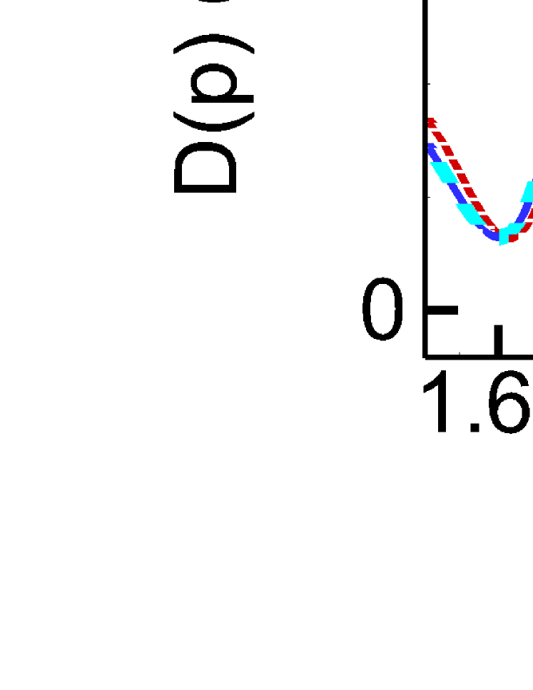
Figure 5: (Color online) The upper row shows the 2D photoelectron momentum distribution $D(\mathbf{p})$ in the $p_{y}$-$p_{z}$ plane ($p_{x}=0$) at $I_{0}=1.0\times 10^{19}~{}\mathrm{W/{cm}^{2}}$: (a) the dipole TDSE calculation for $p_{y}>0$, and (b) the nondipole TDSE calculation for $p_{y}>0$. The lower row shows both the dipole and the nondipole $D(p)$ result for photoelectrons with $p_{x}=0$: (c) along the laser polarization direction, and (d) along the direction of $\theta=\pi/4$.

Then we turn to the phase difference between two electron wave packets ejected in the rising edge and the falling edge, which will interfere with each other and result in the fringe patterns. The ejection time points $t_{1}$ (in the rising edge) and $t_{2}$ (in the falling edge) of the photoelectron with momentum $\bf{p}$ can be obtained by solving Eq. (10). In the period between the time point $t_{1}$ and $t_{2}$, the electron emitted at $t_{1}$ jumps to the Volkov state while the electron emitted at $t_{2}$ remains in the ground state. Due to the nondipole correction to the Volkov phase, a nondipole term needs to be added only to the phase of the electron emitted at $t_{1}$ in this period, which is equal to ${\phi}_{1}(t_{2})-{\phi}_{1}(t_{1})$, see Eq. (8). Therefore the nondipole correction to the phase difference between the two electrons ejected at $t_{1}$ and $t_{2}$ emerges during this period and equals ${\phi}_{1}(t_{1})-{\phi}_{1}(t_{2})$. As a result of the high-frequency oscillation, the phase difference of the two electrons induced by the first term in Eq. (8) is negligible. Therefore the nondipole term added to the phase difference can be expressed as,

$$\Delta\phi=-\frac{A_{0}^{2}p_{x}}{2c}\int_{t_{1}}^{t_{2}}g^{2}(t)dt,$$ (11)

in which the time integration of $A^{2}(t)$ is given by $A_{0}^{2}\int_{t_{1}}^{t_{2}}g^{2}(t)dt$, where $A_{0}$ is the peak value of the vector potential of the whole pulse.

Due to the positive AC-Stark shift of the ground state, the phase of the secondly ejected electron is larger than that of the firstly ejected electron when the two electrons interfere. The larger the ejection time difference is, the greater the phase difference will be. For positive (negative) $p_{x}$, the nondipole correction will decrease (increase) the phase difference, moving the dipole interference fringe to the direction of smaller (larger) momentum value. This finally leads to a momentum shift which is opposite to the laser propagation direction. If the change of the phase difference equals 2$\pi$, the peak positions will be shifted by the fringe spacing $\Delta p_{0}$. For $\Delta\phi$ much smaller than 2$\pi$, we assume the momentum shift depends on $\Delta\phi$ linearly. Then the shift of the peak positions in the momentum spectra can be estimated by,

$$\Delta p_{\text{peak}} =\frac{\Delta\phi}{2\pi}\Delta p_{0}$$ (12)

$$=-\frac{2\int_{t_{1}}^{t_{2}}g^{2}(t)dt}{{\omega}^{2}c^{2}}I_{0}\Delta p_{0}p_{x}.$$

where $I_{0}$ is the laser peak intensity, $\Delta p_{0}$ is the fringe spacing, and $p_{x}$ is the momentum component along the laser propagation direction.

In Eq. (12), it can be seen that the nondipole peak shift is zero if $p_{x}=0$. This is consistent with our TDSE results in Figs. 5(a) and 5(b), where the momentum distributions in the $p_{y}$-$p_{z}$ plane are shown for $p_{x}=0$. In this case, the nondipole effects can indeed be neglected, as can be observed more clearly by looking a line cut in Figs. 5(c) and 5(d). However, for $p_{x}\neq 0$, the nondipole effects will become significant and the momentum shift will depend on the sign of $p_{x}$. According to Eq. (12), $\Delta p_{\text{peak}}$ is negative for electrons with $p_{x}>0$ and positive for $p_{x}<0$. This can explain the different trends of shifts in the momentum space for electrons with positive and negative $p_{x}$ in Figs. 4 (b) and 4(c).

In Fig. 2, the peak positions in the nondipole calculation are roughly located at circles whose center has been shifted away from the origin of coordinates. This shift of center can be approximately deduced from Eq. (12) to be,

$$\Delta p\approx-\frac{2\int_{t_{1}}^{t_{2}}g^{2}(t)dt}{{\omega}^{2}c^{2}}p\Delta p_{0}I_{0}.$$ (13)

For present laser pulses with high intensities, the time points $t_{1}$ and $t_{2}$ of the dominated ejection are located close to the tails of the laser pulse due to the atomic stabilization. Hence in the estimation of Eq. (13), it is possible to approximate $\int_{t_{1}}^{t_{2}}g^{2}(t)dt$ by $\int_{-\infty}^{\infty}g^{2}(t)dt$. The predictions from Eq. (13) are presented as blue crosses in Fig. 3(a), and one can see that they agree very well with the shifts respectively extracted from the TDSE and the semi-analytical model.

IV Conclusions

In summary, by solving the 3D time-dependent Schrödinger equation within/beyond the dipole approximation, we have observed clear dynamic interference exhibited in the ionization of the hydrogen ground state by a super-intense high-frequency laser pulse. The oscillation patterns in the photoelectron energy spectra are controlled by the laser intensity and gradually wiped out in the nondipole calculations. However, through an all-round analysis of the differential momentum distributions of photoelectrons, we find that the smoothing of the peak splitting in the energy spectra is due to momentum shifts in the opposite direction of the laser propagation, which are proportional to the peak laser intensity. By developing a semi-analytical model including the nondipole Volkov phase, all the features observed in the TDSE calculations can be well reproduced. Through an analytic expression for the momentum shift, we point out that the physical origin of this momentum shift can be mainly attributed to the nondipole phase difference between the two electron wave packets ejected in the rising edge and the falling edge. With the fast development of the strong short-wavelength lasers, the predicted phenomena may be observed in the future.