Stochastic comparisons between the extreme claim amounts from two heterogeneous portfolios in the case of transmuted-G model

Abstract

Let $X_{\lambda_{1}},\ldots,X_{\lambda_{n}}$ be independent non-negative random variables belong to the transmuted-G model and let $Y_{i}=I_{p_{i}}X_{\lambda_{i}}$, $i=1,\ldots,n$, where $I_{p_{1}},\ldots,I_{p_{n}}$ are independent Bernoulli random variables independent of $X_{\lambda_{i}}$’s, with ${\rm E}[I_{p_{i}}]=p_{i}$, $i=1,\ldots,n$. In actuarial sciences, $Y_{i}$ corresponds to the claim amount in a portfolio of risks. In this paper we compare the smallest and the largest claim amounts of two sets of independent portfolios belonging to the transmuted-G model, in the sense of usual stochastic order, hazard rate order and dispersive order, when the variables in one set have the parameters $\lambda_{1},...,\lambda_{n}$ and the variables in the other set have the parameters $\lambda^{*}_{1},...,\lambda^{*}_{n}$. For illustration we apply the results to the transmuted-G exponential and the transmuted-G Weibull models.

Keywords Largest claim amount, Majorization, Smallest claim amount, Stochastic ordering.

1 Introduction

Annual premium is the amount paid by the policyholder as the cost of the insurance cover being purchased. Indeed, it is the primary cost to the policyholder for assigning the risk to the insurer which depends on the type of insurance. Determination of the annual premium is one of the important problem in insurance analysis. For this purpose, the smallest and the largest claim amounts play an important role in providing useful information. An attractive problem for the actuaries is expressing preferences between random future gains or losses (Barmalzan et al. bar2 (2017)). For this purpose, stochastic orderings are very helpful. Stochastic orderings have been extensively used in some areas of sciences such as management science, financial economics, insurance, actuarial science, operation research, reliability theory, queuing theory and survival analysis. For more details on stochastic orderings we refer to Müller and Stoyan must (2002), Shaked and Shanthikumar ss (2007) and Li and Li lll (2013). The transmuted-G $({\rm TG})$ model, which introduced by Mirhossaini and Dolati mir2 (2008) and Shaw and Buckley shbu (2009), is an attractive model for constructing new flexible distributions. Let $F$ be an absolutely continuous distribution function with the corresponding survival function ${\bar{F}}$. The random variables $X_{\lambda}$ said to belong to the ${\rm TG}$ model with the baseline distribution function $F$, if $X_{\lambda}$ has the distribution function

$$F_{X_{\lambda}}(x)=F(x)\left(1+\lambda{\bar{F}}(x)\right),$$

where $-1\leq\lambda\leq 1$. We use the notion $X_{\lambda}\thicksim{\rm TG}(\lambda)$ for the transmuted-G model.

Several distributions have been generalized by this transmuting approach in the literature. Some of them are the transmuted Weibull distribution by Aryal and Tsokos arts (2011), the transmuted Maxwell distribution by Iriarte and Astorga iras (2014), the transmuted linear exponential distribution by Tian et al. tian (2014), the transmuted log-logistic distribution by Granzotto and Louzada gr (2015), the transmuted Dagum distribution by Elbatal and Aryal elb (2015), the transmuted Erlang-truncated exponential distribution by Okorie et al. ok (2016), the transmuted exponentiated Weibull geometric distribution by Saboor et al. sab (2016), the transmuted exponential Pareto distribution by Al-Babtain alba (2017), the transmuted two-parameter Lindley distribution by Kemaloglu and Yilmaz keyi (2017) and the transmuted Birnbaum-Saunders distribution by Bourguignon et al. bou (2017).

The problem of stochastic comparisons of some quantities such as the number of claims, the aggregate claim amounts, the smallest and the largest claim amounts in two portfolios, have been considered by many researches in literature; see, e.g., Karlin and Novikoff kar (1963), Ma ma (2000), Frostig fro (2001), Hu and Ruan huru (2004), Denuit and Frostig defr (2006), Khaledi and Ahmadi khah (2008), Zhang and Zhao zz (2015), Barmalzan et al. bar1 (2015), Li and Li lili (2016), Barmalzan and Najafabadi bana (2015), Barmalzan et al. bar3 (2016), Barmalzan et al. bar2 (2017) and Balakrishnan et al. baet (2018). Flexibility of the transmuted-G model is a good property to assuming this model as the distribution of severities in insurance. Motivated by the extensive applications of the transmuted-G family to make flexible models from a given baseline distribution, in this paper we study stochastic comparisons between the extreme claim amounts from two heterogeneous portfolios in the case of transmuted-G model. To be exact, suppose that $X_{\lambda}$ denotes the total random severities of a policyholder in an insurance period, and let $I_{p}$ be a Bernoulli random variable associated with $X_{\lambda}$, such that $I_{p}=1$ whenever the policyholder makes random claim amounts $X_{\lambda}$ and $I_{p}=0$ whenever does not make a claim. In this notation, $Y=I_{p}X_{\lambda}$ is the claim amount in a portfolio of risks. Consider two sets of heterogeneous portfolios $X_{\lambda_{1}},\ldots,X_{\lambda_{n}}$ and $X_{\lambda^{*}_{1}},\ldots,X_{\lambda^{*}_{n}}$ belonging to the TG model and let $Y_{i}=I_{p_{i}}X_{\lambda_{i}}$ and $Y^{*}_{i}=I_{p^{*}_{i}}X_{\lambda^{*}_{i}}$, $i=1,\ldots,n$, where $I_{p_{i}}$ independent of $X_{\lambda_{i}}$ and $I_{p^{*}_{i}}$ independent of $X_{\lambda^{*}_{i}}$ are independent Bernoulli random variables with ${\rm E}[I_{p_{i}}]=p_{i}$ and ${\rm E}[I_{p^{*}_{i}}]=p^{*}_{i}$. Let $Y_{1:n}=\min(Y_{1},\ldots,Y_{n})$, $Y^{*}_{1:n}=\min(Y^{*}_{1},\ldots,Y^{*}_{n})$, $Y_{n:n}=\max(Y_{1},\ldots,Y_{n})$ and $Y^{*}_{n:n}=\max(Y^{*}_{1},\ldots,Y^{*}_{n})$ be the smallest and the largest claim amounts, arise from $Y_{1},\ldots,Y_{n}$ and $Y^{*}_{1},\ldots,Y^{*}_{n}$. In this paper we compare $Y_{1:n}$ and $Y^{*}_{1:n}$ in the sense of the usual stochastic order, hazard rate order and dispersive order and $Y_{n:n}$ and $Y^{*}_{n:n}$ in the sense of the usual stochastic order and hazard rate order. For illustration we apply the results to the transmuted-G exponential and the transmuted-G Weibull models. The rest of the paper is organized as follows. In Section 2, we recall some definitions and lemmas which will be used in the sequel. In Section 3, stochastic comparisons of the largest claim amounts from two heterogeneous portfolios of risks in a transmuted-G model in the sense of the usual stochastic ordering and reversed hazard rate ordering are discussed. In Section 4, stochastic comparisons of the smallest claim amounts from two heterogeneous portfolios of risks in a transmuted-G model in the sense of the usual stochastic ordering, hazard rate ordering and dispersive ordering are discussed. In Section 5 we consider the transmuted-G exponential and the transmuted-G Weibull models for illustration of the established results.

2 The basic definitions and some prerequisites

In this section, we recall some notions of stochastic orderings, majorization, weakly majorization and related orderings and some useful lemmas which are helpful to prove the main results. Throughout the paper, we use the notations $\mathbb{R}=(-\infty,+\infty)$, $\mathbb{R}_{+}=[0,+\infty)$ and $\mathbb{R}_{++}=(0,+\infty)$. The term increasing (decreasing) is used for monotone nondecreasing (nonincreasing). Let $X$ and $Y$ be two non-negative random variables with the respective distribution functions $F$ and $G$, the density functions $f$ and $g$, the survival functions $\bar{F}=1-F$ and $\bar{G}=1-G$, the right continuous inverses $F^{-1}$ and $G^{-1}$, the hazard rate functions $r_{X}={f}/{\bar{F}}$ and $r_{Y}={g}/{\bar{G}}$, and the reversed hazard rate functions $\tilde{r}_{X}={f}/{F}$ and $\tilde{r}_{Y}={g}/{G}$.

Definition 2.1.

$X$ is said to be smaller than $Y$ in the

• usual stochastic ordering, denoted by $X\leq_{\rm st}Y$, if $\bar{F}(x)\leq\bar{G}(x)$ for all $x\in\mathbb{R}$,

• hazard rate ordering, denoted by $X\leq_{\rm hr}Y$, if ${\bar{G}}(x)/{\bar{F}}(x)$ is increasing in $x\in\mathbb{R}$, or $r_{Y}(x)\leq r_{X}(x)$ for all $x\in\mathbb{R}$,

• reversed hazard rate ordering, denoted by $X\leq_{\rm rh}Y$, if $G(x)/F(x)$ is increasing in $x\in\mathbb{R}_{+}$, or $\tilde{r}_{X}(x)\leq\tilde{r}_{Y}(x)$ for all $x\in\mathbb{R}_{+}$,

• dispersive ordering, denoted by $X\leq_{\rm disp}Y$, if $F^{-1}(\beta)-F^{-1}(\alpha)\leq G^{-1}(\beta)-G^{-1}(\alpha)$ for all $0\leq\alpha\leq\beta\leq 1$.

We know that the hazard rate and reversed hazard rate orderings imply the usual stochastic ordering.

Lemma 2.1 (Shaked and Shanthikumarss (2007), Theorem 3.B.20).

Let $X$ and $Y$ be two non-negative random variables. If $X\leq_{{\rm hr}}Y$ and $X$ or $Y$ is decreasing failure rate (DFR), then $X\leq_{{\rm disp}}Y$.

For a comprehensive discussion on various stochastic orderings, we refer to Li and Li lll (2013) and Shaked and Shanthikumar ss (2007).

We also need the concept of majorization of vectors and matrices and the Schur-convexity and Schur-concavity of functions. For a comprehensive discussion of these topics we refer to Marshall et al. met (2011). We use the notation $x_{(1)}\leq x_{(2)}\leq...\leq x_{(n)}$ to denote the increasing arrangement of the components of the vector $\boldsymbol{x}=(x_{1},\ldots,x_{n})$.

Definition 2.2.

The vector $\boldsymbol{x}$ is said to be

• weakly submajorized by the vector $\boldsymbol{y}$ (denoted by $\boldsymbol{x}\preceq_{\rm w}\boldsymbol{y}$) if $\sum_{i=j}^{n}x_{(i)}\leq\sum_{i=j}^{n}y_{(i)}$ for all $j=1,\ldots,n$,

• weakly supermajorized by the vector $\boldsymbol{y}$ (denoted by $\boldsymbol{x}\mathop{\preceq}\limits^{{\mathop{\rm w}}}\boldsymbol{y}$) if $\sum_{i=1}^{j}x_{(i)}\geq\sum_{i=1}^{j}y_{(i)}$ for all $j=1,\ldots,n$,

• majorized by the vector $\boldsymbol{y}$ (denoted by $\boldsymbol{x}\mathop{\preceq}\limits^{{\mathop{\rm m}}}\boldsymbol{y}$) if $\sum_{i=1}^{n}x_{i}=\sum_{i=1}^{n}y_{i}$ and $\sum_{i=1}^{j}x_{(i)}\geq\sum_{i=1}^{j}y_{(i)}$ for all $j=1,\ldots,n-1$.

Definition 2.3.

A real valued function $\varphi$ defined on a set $\mathscr{A}\subseteq{\mathbb{R}}^{n}$ is said to be Schur-convex (Schur-concave) on $\mathscr{A}$ if

$$\boldsymbol{x}\mathop{\preceq}\limits^{{\mathop{\rm m}}}\boldsymbol{y}\quad\text{on}\quad\mathscr{A}\Longrightarrow\varphi(\boldsymbol{x})\leq(\geq)\varphi(\boldsymbol{y}).$$

Lemma 2.2 (Marshall et al.met (2011), Theorem 3.A.4).

Let $\mathscr{A}\subseteq\mathbb{R}$ be an open interval and let $l:\mathscr{A}^{n}\rightarrow\mathbb{R}$ be continuously differentiable. $l$ is Schur-convex (Schur-concave) on $\mathscr{A}^{n}$ if and only if, $l$ is symmetric on $\mathscr{A}^{n}$ and for all $i\neq j$,

$$(x_{i}-x_{j})\left(\frac{\partial{l(\boldsymbol{x})}}{\partial{x_{i}}}-\frac{\partial{l(\boldsymbol{x})}}{\partial{x_{j}}}\right)\geq(\leq)0,\quad\text{for all}\quad\boldsymbol{x}\in\mathscr{A}^{n}.$$

Lemma 2.3 (Marshall et al.met (2011), Theorem 3.A.8).

For a function $l$ on $\mathscr{A}\subseteq\mathbb{R}^{n}$, $\boldsymbol{x}\preceq_{\rm w}\boldsymbol{y}$ implies $l(\boldsymbol{x})\leq(\geq)l(\boldsymbol{y})$ if and only if it is increasing (decreasing) and Schur-convex (Schur-concave) on $\mathscr{A}$.

In the following we recall the concepts of $T$-transform matrix and chain majorization of matrices. We refer to Marshall et al. met (2011) for more details.

Definition 2.4.

A square matrix is called a

• permutation matrix if each row and each column has a single unit, and all other entries are zero,

• $T$-transform matrix if it is of the form $T_{\omega}=\omega I_{n}+(1-\omega)\Pi$, where $0\leq\omega\leq 1$, $I_{n}$ is an $n\times n$ identity matrix and $\Pi$ is a permutation matrix that just interchanges two coordinates.

Two $T$-transform matrices said to have the same structure if their permutation matrices are identical; otherwise they said to have different structures.

In the following definition, we recall a multivariate majorization notion which will be used in the sequel.

Definition 2.5.

Let $A=\{a_{ij}\}$ and $B=\{b_{ij}\}$ be two $m\times n$ matrices. Then $A$ is said to be chain majorized by $B$, denoted by $A\ll B$, if there exists a finite set of $n\times n$ $T$-transform matrices $T_{\omega_{1}},\ldots,T_{\omega_{k}}$ such that $A=BT_{\omega_{1}}\times\ldots\times T_{\omega_{k}}$.

For $i=1,\ldots,m$ , let $\boldsymbol{a}^{R}_{i}$ and $\boldsymbol{b}^{R}_{i}$, denote the $i$th row of $A$ and $B$, respectively. Then we have

$A\ll B$	$\Rightarrow$	$\boldsymbol{a}^{R}_{i}\mathop{\preceq}\limits^{{\mathop{\rm m}}}\boldsymbol{b}^{R}_{i}$	$\Rightarrow$	$\boldsymbol{a}^{R}_{i}\preceq_{\rm w}\boldsymbol{b}^{R}_{i}$
		$\Downarrow$
		$\boldsymbol{a}^{R}_{i}\mathop{\preceq}\limits^{{\mathop{\rm w}}}\boldsymbol{b}^{R}_{i}$	$\Rightarrow$	$\prod\limits_{j=1}^{n}b_{ij}\leq\prod\limits_{j=1}^{n}a_{ij}$,

where the last consequence holds whenever $\boldsymbol{a}^{R}_{i},\boldsymbol{b}^{R}_{i}\in\mathbb{R}^{n}_{++}$. Let

$$S_{n}=\bigg{\{}(\boldsymbol{x},\boldsymbol{y})=\begin{bmatrix}x_{1},\ldots,x_{n}\\ y_{1},\ldots,y_{n}\end{bmatrix}:-1\leq x_{i}\leq 1,y_{i}>0,\text{and}\quad(x_{i}-x_{j})(y_{i}-y_{j})\leq 0,$$

$\hskip 56.9055pti,j=1,\dots,n\bigg{\}}.$

We recall the following lemmas similar to the lemmas in Balakrishnan et al.bee (2015), which their proofs are very similar to the proofs of lemmas in Balakrishnan et al.bee (2015). So, the proofs are omitted for simplicity.

Lemma 2.4.

A differentiable function $\varphi:\mathbb{R}^{4}\longrightarrow\mathbb{R}_{+}$ satisfies

$$\varphi(A)\leq\varphi(B)\text{ for all }A,B\text{ such that }B\in S_{2},\text{ and }A\ll B$$ (1)

if and only if

• $\varphi(B)=\varphi(B\Pi)$ for all permutation matrices $\Pi$, and all $B\in S_{2}$; and

• $\sum_{i=1}^{2}(b_{ik}-b_{ij})(\varphi_{ik}(B)-\varphi_{ij}(B))\geq 0$ for all $j,k=1,2$, and all $B\in S_{2}$, where $\varphi_{ij}(B)=\dfrac{\partial\varphi(B)}{\partial b_{ij}}$.

Lemma 2.5.

Let $\Psi:\mathbb{R}^{2}\longrightarrow\mathbb{R}_{+}$ be a differentiable function, and let the function $\upsilon_{n}:\mathbb{R}^{2n}\longrightarrow\mathbb{R}_{+}$ defined by

$$\upsilon_{n}(B)=\prod_{i=1}^{n}\Psi(b_{1i},b_{2i}).$$

If $\upsilon_{2}$ satisfies (1), then, for $B\in S_{n}$, and $A=BT_{\omega}$, we have $\upsilon_{n}(A)\leq\upsilon_{n}(B)$.

Lemma 2.6.

Let $k$ be a function defined by

$$k(x,y,z):=\frac{x}{1-xyz}.$$

Then,

• $k$ is increasing in $x$,

• $k$ is increasing in $y$, when $z\geq 0$.

3 Results for the largest claim amounts

It is clear that the random variables $Y_{i}=I_{p_{i}}X_{\lambda_{i}}$, $i=1,\ldots,n$, are discrete-continuous, which are equal to zero with the probability $1-p_{i}$, and $X_{\lambda_{i}}$ with the probability $p_{i}$, $i=1,\ldots,n$. The distribution function and the reversed hazard rate function of $Y_{n:n}$, the largest claim amount, are given by

$$G_{Y_{n:n}}(x)=\prod\limits_{i=1}^{n}\Bigg{(}1-p_{i}{\bar{F}}(x)\Big{(}1-\lambda_{i}F(x)\Big{)}\Bigg{)},\quad x\geq 0.$$ (2)

and

$$\tilde{r}_{Y_{n:n}}(x)=\sum\limits_{i=1}^{n}\frac{f(x)\Big{(}1+\lambda_{i}(1-2F(x))\Big{)}p_{i}}{1-p_{i}{\bar{F}}(x)\left(1-\lambda_{i}F(x)\right)}{\rm I}_{[x>0]}+{\rm I}_{[x=0]},$$ (3)

respectively; where ${\rm I}_{A}$ denotes the indicator function. Similarly, the distribution function and the reversed hazard rate function of $Y^{*}_{n:n}$ is the same as in (2) and (3) upon replacing $\lambda_{i}$ by $\lambda^{*}_{i}$ and $p_{i}$ by $p^{*}_{i}$, $i=1,\ldots,n$, respectively.

The following theorem provides a comparison between the largest claim amounts in two heterogeneous portfolio of risks, in the sense of the usual stochastic ordering via matrix majorization.

Theorem 3.1.

Let $X_{\lambda_{1}},X_{\lambda_{2}}$ ($X_{\lambda^{*}_{1}},X_{\lambda^{*}_{2}}$) be independent non-negative random variables with $X_{\lambda_{i}}\thicksim{\rm TG}(\lambda_{i})$ ($X_{\lambda^{*}_{i}}\thicksim{\rm TG}(\lambda^{*}_{i})$), $i=1,2$. Further, suppose that $I_{p_{1}},I_{p_{2}}$ ($I_{p^{*}_{1}},I_{p^{*}_{2}}$) is a set of independent Bernoulli random variables, independent of the $X_{\lambda_{i}}$’s ($X_{\lambda^{*}_{i}}$’s), with ${\rm E}[I_{p_{i}}]=p_{i}$ (${\rm E}[I_{p^{*}_{i}}]=p^{*}_{i}$), $i=1,2$. Let $h:[0,1]\rightarrow I\subset\mathbb{R}_{+}$ be a differentiable and strictly increasing concave function on $[0,1]$ with the non-zero derivative. Then for $(\boldsymbol{\lambda},h(\boldsymbol{p}))\in S_{2}$, we have

$$\begin{bmatrix}\lambda^{*}_{1}&\lambda^{*}_{2}\\ h(p^{*}_{1})&h(p^{*}_{2})\\ \end{bmatrix}\ll\begin{bmatrix}\lambda_{1}&\lambda_{2}\\ h(p_{1})&h(p_{2})\\ \end{bmatrix}\Longrightarrow Y^{*}_{2:2}\leq_{\rm st}Y_{2:2}.$$

Proof.

In view of (2), the distribution function of $Y_{2:2}$ can be rewritten as

$$G_{Y_{2:2}}(x)=\prod\limits_{i=1}^{2}\Bigg{(}1-h^{-1}(u_{i}){\bar{F}}(x)\Big{(}1-\lambda_{i}F(x)\Big{)}\Bigg{)},\quad x\geq 0,$$

where $h^{-1}$ is the inverse of the function $h$, and $u_{i}=h(p_{i})$, $i=1,2$. For fixed $x\geq 0$, we have to show that the function $G_{Y_{2:2}}(x)$ satisfies the conditions of Lemma 2.4. Clearly, the condition (i) is satisfied. To check the condition (ii), consider the function $\rho$ given by

$$\rho(\boldsymbol{\lambda},\boldsymbol{u})=\rho_{1}(\boldsymbol{\lambda},\boldsymbol{u})+\rho_{2}(\boldsymbol{\lambda},\boldsymbol{u}),$$ (4)

where

$$\rho_{1}(\boldsymbol{\lambda},\boldsymbol{u})=(u_{1}-u_{2})\bigg{(}\dfrac{\partial G_{Y_{2:2}}(x)}{\partial u_{1}}-\dfrac{\partial G_{Y_{2:2}}(x)}{\partial u_{2}}\bigg{)},$$

and

$$\rho_{2}(\boldsymbol{\lambda},\boldsymbol{u})=(\lambda_{1}-\lambda_{2})\bigg{(}\dfrac{\partial G_{Y_{2:2}}(x)}{\partial\lambda_{1}}-\dfrac{\partial G_{Y_{2:2}}(x)}{\partial\lambda_{2}}\bigg{)}.$$

The partial derivatives of $G_{Y_{2:2}}(x)$ with respect to $u_{i}$ and $\lambda_{i}$ are given by

$$\dfrac{\partial G_{Y_{2:2}}(x)}{\partial u_{i}}=-\frac{(1-\lambda_{i}F(x))\frac{\partial h^{-1}(u_{i})}{\partial u_{i}}}{1-h^{-1}(u_{i}){\bar{F}}(x)\left(1-\lambda_{i}F(x)\right)}{\bar{F}}(x)G_{Y_{2:2}}(x),$$

and

$$\dfrac{\partial G_{Y_{2:2}}(x)}{\partial\lambda_{i}}=\frac{h^{-1}(u_{i})}{1-h^{-1}(u_{i}){\bar{F}}(x)\left(1-\lambda_{i}F(x)\right)}F(x){\bar{F}}(x)G_{Y_{2:2}}(x).$$

Thus

$$\rho_{1}(\boldsymbol{\lambda},\boldsymbol{u})=-(u_{1}-u_{2}){\bar{F}}(x)G_{Y_{2:2}}(x)\left(\eta_{1}(\lambda_{1},u_{1})\frac{\partial h^{-1}(u_{1})}{\partial u_{1}}-\eta_{1}(\lambda_{2},u_{2})\frac{\partial h^{-1}(u_{2})}{\partial u_{2}}\right),$$

where, $\eta_{1}(\lambda,u)=k\left(1-\lambda F(x),h^{-1}(u),{\bar{F}}(x)\right)$, and $k$ is the function defined in Lemma 2.6. The assumption $(\boldsymbol{\lambda},\boldsymbol{u})\in S_{2}$ implies that $(\lambda_{1}-\lambda_{2})(u_{1}-u_{2})\leq 0$ or equivalently, $\lambda_{1}\leq\lambda_{2}$ and $u_{1}\geq u_{2}$, or $\lambda_{1}\geq\lambda_{2}$ and $u_{1}\leq u_{2}$. We only state the proof for the case $\lambda_{1}\leq\lambda_{2}$ and $u_{1}\geq u_{2}$. The other case is analogously proven. Since $h$ is strictly increasing and concave then $h^{-1}$ is strictly increasing and convex. The convexity of $h^{-1}$ implies that

$$0\leq\frac{\partial h^{-1}(u_{2})}{\partial u_{2}}\leq\frac{\partial h^{-1}(u_{1})}{\partial u_{1}}.$$

In view of Lemma 2.6 the function $\eta_{1}$ is decreasing in $\lambda$ and increasing in $u$, so that

$$0\leq\eta_{1}(\lambda_{2},u_{2})\leq\eta_{1}(\lambda_{1},u_{2})\leq\eta_{1}(\lambda_{1},u_{1}),$$

which implies that

$$\rho_{1}(\boldsymbol{\lambda},\boldsymbol{u})\leq 0.$$ (5)

On the other hand,

$$\rho_{2}(\boldsymbol{\lambda},\boldsymbol{u})=(\lambda_{1}-\lambda_{2})F(x){\bar{F}}(x)G_{Y_{2:2}}(x)\Big{(}\eta_{2}(\lambda_{1},u_{1})-\eta_{2}(\lambda_{2},u_{2})\Big{)},$$

where, $\eta_{2}(\lambda,u)=k\left(h^{-1}(u),1-\lambda F(x),{\bar{F}}(x)\right)$. By a similar argument the function $\eta_{2}$ is decreasing in $\lambda$ and increasing in $u$ and

$$\eta_{2}(\lambda_{2},u_{2})\leq\eta_{2}(\lambda_{1},u_{2})\leq\eta_{2}(\lambda_{1},u_{1}),$$

which implies that

$$\rho_{2}(\boldsymbol{\lambda},\boldsymbol{u})\leq 0.$$ (6)

By using the inequalities (4), (5) and (6), we have that

$$\rho(\boldsymbol{\lambda},\boldsymbol{u})\leq 0,$$

and the function $G_{Y_{2:2}}(x)$ satisfies the condition (ii) of Lemma 2.4. Now Lemma 2.4 and the condition $(\boldsymbol{\lambda}^{*},\boldsymbol{u}^{*})\ll(\boldsymbol{\lambda},\boldsymbol{u})$ implies that

$$G_{Y_{2:2}}(x)\leq G_{Y^{*}_{2:2}}(x),$$

which is the required result. ∎

The following result provides a lower bound for the survival function of the largest claim amount based on a heterogeneous portfolio of risks in terms of the survival function of largest claim amounts based on a homogeneous portfolio of risks.

Corollary 3.1.

Let $\bar{\lambda}=\frac{1}{2}(\lambda_{1}+\lambda_{2})$ and $\overline{h(p)}=\frac{1}{2}(h(p_{1})+h(p_{2}))$. Under the conditions of Theorem 3.1 we have

$${\bar{G}}_{Y_{2:2}}(x)\geq 1-\Bigg{(}1-h^{-1}(\overline{h(p)}){\bar{F}}(x)\Big{(}1-\bar{\lambda}F(x)\Big{)}\Bigg{)}^{2}.$$

Proof.

It is clear that $\begin{bmatrix}\bar{\lambda}&\bar{\lambda}\\ \overline{h(p)}&\overline{h(p)}\\ \end{bmatrix}=\begin{bmatrix}\lambda_{1}&\lambda_{2}\\ h(p_{1})&h(p_{2})\\ \end{bmatrix}T_{0.5}$. Thus we have $\begin{bmatrix}\bar{\lambda}&\bar{\lambda}\\ \overline{h(p)}&\overline{h(p)}\\ \end{bmatrix}\ll\begin{bmatrix}\lambda_{1}&\lambda_{2}\\ h(p_{1})&h(p_{2})\\ \end{bmatrix}$. Now Theorem 2.4 gives the required result. ∎

The following result generalizes the result of Theorem 2.4 for an arbitrary number of random variables.

Theorem 3.2.

Let $X_{\lambda_{1}},\ldots,X_{\lambda_{n}}$ ($X_{\lambda^{*}_{1}},\ldots,X_{\lambda^{*}_{n}}$) be independent non-negative random variables with $X_{\lambda_{i}}\thicksim{\rm TG}(\lambda_{i})$ ($X_{\lambda^{*}_{i}}\thicksim{\rm TG}(\lambda^{*}_{i})$), $i=1,\ldots,n$. Further, suppose that $I_{p_{1}},\ldots,I_{p_{n}}$ ($I_{p^{*}_{1}},\ldots,I_{p^{*}_{n}}$) is a set of independent Bernoulli random variables, independent of the $X_{\lambda_{i}}$’s ($X_{\lambda^{*}_{i}}$’s), with ${\rm E}[I_{p_{i}}]=p_{i}$ (${\rm E}[I_{p^{*}_{i}}]=p^{*}_{i}$), $i=1,\ldots,n$. Let $h:[0,1]\rightarrow I\subset\mathbb{R}_{+}$ be a differentiable and strictly increasing concave function on $[0,1]$, with non-zero derivative. Then for $(\boldsymbol{\lambda},h(\boldsymbol{p}))\in S_{n}$, we have

$$\begin{bmatrix}\lambda^{*}_{1}&\ldots&\lambda^{*}_{n}\\ h(p^{*}_{1})&\ldots&h(p^{*}_{n})\\ \end{bmatrix}=\begin{bmatrix}\lambda_{1}&\ldots&\lambda_{n}\\ h(p_{1})&\ldots&h(p_{n})\\ \end{bmatrix}T_{\omega}\Longrightarrow Y^{*}_{n:n}\leq_{\rm st}Y_{n:n}.$$

Proof.

Using Lemma 2.5 and Theorem 3.1, we immediately obtain the required result. ∎

According to Balakrishnan et al.bee (2015), a finite product of $T$-transform matrices with the same structure is also a $T$-transform matrix. Thus the following result is a direct consequence of Theorem 3.2.

Corollary 3.2.

Under the assumptions of Theorem 3.2, for $(\boldsymbol{\lambda},h(\boldsymbol{p}))\in S_{n}$, we have

$$\begin{bmatrix}\lambda^{*}_{1}&\ldots&\lambda^{*}_{n}\\ h(p^{*}_{1})&\ldots&h(p^{*}_{n})\\ \end{bmatrix}=\begin{bmatrix}\lambda_{1}&\ldots&\lambda_{n}\\ h(p_{1})&\ldots&h(p_{n})\\ \end{bmatrix}T_{\omega_{1}}\ldots T_{\omega_{m}}\Longrightarrow Y^{*}_{n:n}\leq_{\rm st}Y_{n:n},$$

where $T_{\omega_{i}}$, $i=1,\ldots,m$, have the same structure.

The following corollary provides a result for the case where the $T$-transform matrices have different structures.

Corollary 3.3.

Under the assumptions of Theorem 3.2, for $(\boldsymbol{\lambda},h(\boldsymbol{p}))\in S_{n}$, and $(\boldsymbol{\lambda},h(\boldsymbol{p}))T_{\omega_{1}},\ldots,T_{\omega_{i}}\in S_{n}$, for $i=1,\ldots,m-1$, where $m\geq 2$, we have

$$\begin{bmatrix}\lambda^{*}_{1}&\ldots&\lambda^{*}_{n}\\ h(p^{*}_{1})&\ldots&h(p^{*}_{n})\\ \end{bmatrix}=\begin{bmatrix}\lambda_{1}&\ldots&\lambda_{n}\\ h(p_{1})&\ldots&h(p_{n})\\ \end{bmatrix}T_{\omega_{1}}\ldots T_{\omega_{m}}\Longrightarrow Y^{*}_{n:n}\leq_{\rm st}Y_{n:n},$$

Proof.

Using Theorem 3.2 consecutively, the desired result is immediately obtained. ∎

The following result deals with the comparison of the largest claim amounts in a homogeneous portfolio of risks, in the sense of the reversed hazard rate ordering via weakly majorization.

Theorem 3.3.

Under the assumptions of Theorem 3.2 with $\lambda_{i}=\lambda^{*}_{i}=\lambda$, for $i=1,\ldots,n$, we have

$$(h(p^{*}_{1}),\ldots,h(p^{*}_{n}))\preceq_{{\rm w}}(h(p_{1}),\ldots,h(p_{n}))\Longrightarrow Y^{*}_{n:n}\leq_{{\rm rh}}Y_{n:n}.$$

Proof.

According to (3), the reversed hazard rate function of $Y_{n:n}$ can be rewritten as

$$\tilde{r}_{Y_{n:n}}(x)=\sum_{i=1}^{n}\frac{f(x)\Big{(}1+\lambda(1-2F(x))\Big{)}h^{-1}(u_{i})}{1-h^{-1}(u_{i}){\bar{F}}(x)\left(1-\lambda F(x)\right)}{\rm I}_{[x>0]}+{\rm I}_{[x=0]},$$

where, $u_{i}=h(p_{i})$, $i=1,\ldots,n$. First, consider $x=0$. In this case, $\tilde{r}_{Y_{n:n}}(0)=\tilde{r}_{Y^{*}_{n:n}}(0)=1$, and the desired result is obvious. Now, consider $x>0$. Using Lemma 2.3, it is enough to show that the function $\tilde{r}_{Y_{n:n}}(x)$ is Schur-convex and increasing in $u_{i}$’s. The partial derivatives of $\tilde{r}_{Y_{n:n}}(x)$ with respect to $u_{i}$ is given by

$$\frac{\partial\tilde{r}_{Y_{n:n}}(x)}{\partial{u_{i}}}=\frac{f(x)\Big{(}1+\lambda(1-2F(x))\Big{)}\frac{\partial h^{-1}(u_{i})}{\partial u_{i}}}{\bigg{(}1-h^{-1}(u_{i}){\bar{F}}(x)\left(1-\lambda F(x)\right)\bigg{)}^{2}}\geq 0.$$

Thus, $\tilde{r}_{Y_{n:n}}(x)$ is increasing in each $u_{i}$. To prove the Schur-convexity of $\tilde{r}_{Y_{n:n}}(x)$, from Lemma 2.2, it is enough to show that for $i\neq j$,

$$(u_{i}-u_{j})\bigg{(}\frac{\partial\tilde{r}_{Y_{n:n}}(x)}{\partial u_{i}}-\frac{\partial\tilde{r}_{Y_{n:n}}(x)}{\partial u_{j}}\bigg{)}\geq 0,$$

that is, for $i\neq j$,

$$(u_{i}-u_{j})f(x)\Big{(}1+\lambda(1-2F(x))\Big{)}$$

$$\times\Bigg{(}\frac{\frac{\partial h^{-1}(u_{i})}{\partial u_{i}}}{\bigg{(}1-h^{-1}(u_{i}){\bar{F}}(x)\left(1-\lambda F(x)\right)\bigg{)}^{2}}-\frac{\frac{\partial h^{-1}(u_{j})}{\partial u_{j}}}{\bigg{(}1-h^{-1}(u_{j}){\bar{F}}(x)\left(1-\lambda F(x)\right)\bigg{)}^{2}}\Bigg{)}\geq 0.$$

Since $h$ is increasing and concave, then $h^{-1}$ is increasing and convex. Thus, the inequality immediately holds. ∎

4 Results for the smallest claim amounts

It can be easily seen that the survival function and the hazard rate function of $Y_{1:n}$, the smallest claim amount, are given by

$${\bar{G}}_{Y_{1:n}}(x)=\Bigg{(}\prod\limits_{i=1}^{n}p_{i}\Bigg{)}\prod\limits_{i=1}^{n}\Bigg{(}{\bar{F}}(x)\big{(}1-\lambda_{i}F(x)\big{)}\Bigg{)},\quad x\geq 0,$$ (7)

and

$$r_{Y_{1:n}}(x)=\sum_{i=1}^{n}\frac{1+\lambda_{i}(1-2F(x))}{1-\lambda_{i}F(x)}r(x){\rm I}_{[x>0]}+\left(1-\prod\limits_{i=1}^{n}p_{i}\right){\rm I}_{[x=0]},$$ (8)

respectively. Similarly, the survival function and the hazard rate function of $Y^{*}_{1:n}$ is the same as in (7) and (8) upon replacing $\lambda_{i}$ by $\lambda^{*}_{i}$ and $p_{i}$ by $p^{*}_{i}$, $i=1,\ldots,n$, respectively.

The following result deals with the comparison of the smallest claim amounts in a portfolio of risks, in the sense of the usual stochastic ordering via majorization.

Theorem 4.1.

Let $X_{\lambda_{1}},\ldots,X_{\lambda_{n}}$ ($X_{\lambda^{*}_{1}},\ldots,X_{\lambda^{*}_{n}}$) be independent non-negative random variables with $X_{\lambda_{i}}\thicksim{\rm TG}(\lambda_{i})$ ($X_{\lambda^{*}_{i}}\thicksim{\rm TG}(\lambda^{*}_{i})$), $i=1,\ldots,n$. Further, suppose that $I_{p_{1}},\ldots,I_{p_{n}}$ ($I_{p^{*}_{1}},\ldots,I_{p^{*}_{n}}$) is a set of independent Bernoulli random variables, independent of the $X_{\lambda_{i}}$’s ($X_{\lambda^{*}_{i}}$’s), with ${\rm E}[I_{p_{i}}]=p_{i}$ (${\rm E}[I_{p^{*}_{i}}]=p^{*}_{i}$), $i=1,\ldots,n$. Then, we have

$$\prod\limits_{i=1}^{n}p^{*}_{i}\leq\prod\limits_{i=1}^{n}p_{i},~{}(\lambda_{1},\ldots,\lambda_{n})\preceq_{{\rm w}}(\lambda^{*}_{1},\ldots,\lambda^{*}_{n})\Longrightarrow Y^{*}_{1:n}\leq_{\rm st}Y_{1:n}.$$

Proof.

Assume that $\prod\limits_{i=1}^{n}p^{*}_{i}\leq\prod\limits_{i=1}^{n}p_{i}$. Now using (7), the required result holds if $X^{*}_{1:n}\leq_{\rm st}X_{1:n}$, where $X^{*}_{1:n}$ and $X_{1:n}$ are the smallest order statistics of $(X_{\lambda^{*}_{1}},\ldots,X_{\lambda^{*}_{n}})$ and $(X_{\lambda_{1}},\ldots,X_{\lambda_{n}})$, respectively. The survival function of $X_{1:n}$ is given by

$${\bar{F}}_{X_{1:n}}(x)=\prod\limits_{i=1}^{n}\Bigg{(}{\bar{F}}(x)\big{(}1-\lambda_{i}F(x)\big{)}\Bigg{)},\quad x\geq 0.$$

Thus by Lemma 2.3, it is enough to show that the function ${\bar{F}}_{X_{1:n}}(x)$ is Schur-concave and decreasing in $\lambda_{i}$’s. The partial derivative of ${\bar{F}}_{X_{1:n}}(x)$ with respect to $\lambda_{i}$ is given by

$$\frac{\partial{\bar{F}}_{X_{1:n}}(x)}{\partial\lambda_{i}}=-\frac{F(x){\bar{F}}_{X_{1:n}}(x)}{1-\lambda_{i}F(x)}\leq 0.$$

Thus ${\bar{F}}_{X_{1:n}}(x)$ is decreasing in each $\lambda_{i}$. To prove the Schur-concavity of ${\bar{F}}_{X_{1:n}}(x)$, from Lemma 2.2, it is enough to show that for $i\neq j$,

$$(\lambda_{i}-\lambda_{j})\bigg{(}\frac{\partial{\bar{F}}_{X_{1:n}}(x)}{\partial\lambda_{i}}-\frac{\partial{\bar{F}}_{X_{1:n}}(x)}{\partial\lambda_{j}}\bigg{)}\leq 0,$$

that is, for $i\neq j$,

$$-(\lambda_{i}-\lambda_{j})F(x){\bar{F}}_{X_{1:n}}(x)\bigg{(}\frac{1}{1-\lambda_{i}F(x)}-\frac{1}{1-\lambda_{j}F(x)}\bigg{)}\leq 0,$$

which is immediately concluded. ∎

The following result provides a lower bound for the survival function of the smallest claim amount based on a heterogeneous portfolio of risks in terms of the survival function of smallest claim amounts based on a homogeneous portfolio of risks.

Corollary 4.1.

Under the assumption of Theorem 4.1

$${\bar{G}}_{Y_{1:n}}(x)\geq\Bigg{(}\tilde{p}{\bar{F}}(x)\big{(}1-\tilde{\lambda}F(x)\big{)}\Bigg{)}^{n},$$

where $\prod\limits_{i=1}^{n}p_{i}=\tilde{p}^{n}$ and $\tilde{\lambda}=\max\bigg{(}\frac{1}{2}(1+\lambda_{1}),\ldots,\frac{1}{2}(1+\lambda_{n})\bigg{)}$.

Proof.

It is clear that

$$(\lambda_{1},\ldots,\lambda_{n})\preceq_{{\rm w}}\bigg{(}\frac{1}{2}(1+\lambda_{1}),\ldots,\frac{1}{2}(1+\lambda_{n})\bigg{)}\preceq_{{\rm w}}(\tilde{\lambda},\ldots,\tilde{\lambda}).$$

These assumptions satisfy the conditions of Theorem 4.1, which implies the result. ∎

The following result shows that under the same conditions of Theorem 4.1, a stronger result also holds.

Theorem 4.2.

Under the assumptions of Theorem 4.1, we have

$$\prod\limits_{i=1}^{n}p^{*}_{i}\leq\prod\limits_{i=1}^{n}p_{i},~{}(\lambda_{1},\ldots,\lambda_{n})\preceq_{{\rm w}}(\lambda^{*}_{1},\ldots,\lambda^{*}_{n})\Longrightarrow Y^{*}_{1:n}\leq_{\rm hr}Y_{1:n}.$$

Proof.

According to (7), we have

$$\frac{{\bar{G}}_{Y_{1:n}}(x)}{{\bar{G}}_{Y^{*}_{1:n}}(x)}=\left(\frac{\prod\limits_{i=1}^{n}p_{i}}{\prod\limits_{i=1}^{n}p^{*}_{i}}\right)\frac{{\bar{F}}_{X_{1:n}}(x)}{{\bar{F}}_{X^{*}_{1:n}}(x)},\quad x\geq 0.$$

We have to show that $\frac{{\bar{G}}_{Y_{1:n}}(x)}{{\bar{G}}_{Y^{*}_{1:n}}(x)}$ is increasing in $x$, which holds if

$$1=\lim\limits_{{\mathop{x\rightarrow 0^{-}}}}\frac{{\bar{G}}_{Y_{1:n}}(x)}{{\bar{G}}_{Y^{*}_{1:n}}(x)}\leq\frac{{\bar{G}}_{Y_{1:n}}(0)}{{\bar{G}}_{Y^{*}_{1:n}}(0)}=\frac{\prod\limits_{i=1}^{n}p_{i}}{\prod\limits_{i=1}^{n}p^{*}_{i}},$$ (9)

and $\frac{{\bar{F}}_{X_{1:n}}(x)}{{\bar{F}}_{X^{*}_{1:n}}(x)}$ is increasing in $x$. Since Inequality (9) holds according to the assumptions, it is enough to show that $X^{*}_{1:n}\leq_{\rm hr}X_{1:n}$ or equivalently $r_{X_{1:n}}(x)\leq r_{X^{*}_{1:n}}(x)$, for $x\geq 0$. The hazard rate function of $X_{1:n}$ is given by

$$r_{X_{1:n}}(x)=\sum\limits_{i=1}^{n}\frac{1+\lambda_{i}\left(1-2F(x)\right)}{1-\lambda_{i}F(x)}r(x),\quad x\geq 0.$$

Thus by Lemma 2.3, it is enough to show that the function $r_{X_{1:n}}(x)$ is Schur-convex and increasing in $\lambda_{i}$’s. The partial derivative of $r_{X_{1:n}}(x)$ with respect to $\lambda_{i}$ is given by

$$\frac{\partial r_{X_{1:n}}(x)}{\partial\lambda_{i}}=\frac{{\bar{F}}(x)r(x)}{(1-\lambda_{i}F(x))^{2}}\geq 0.$$

Thus $r_{X_{1:n}}(x)$ is increasing in each $\lambda_{i}$. To prove the Schur-convexity of $r_{X_{1:n}}(x)$, from Lemma 2.2, it is enough to show that for $i\neq j$,

$$(\lambda_{i}-\lambda_{j})\bigg{(}\frac{\partial r_{X_{1:n}}(x)}{\partial\lambda_{i}}-\frac{\partial r_{X_{1:n}}(x)}{\partial\lambda_{j}}\bigg{)}\geq 0,$$

that is, for $i\neq j$,

$$(\lambda_{i}-\lambda_{j}){\bar{F}}(x)r(x)\bigg{(}\frac{1}{(1-\lambda_{i}F(x))^{2}}-\frac{1}{(1-\lambda_{j}F(x))^{2}}\bigg{)}\geq 0,$$

where, the inequality is immediately concluded. ∎

The following result deals with the comparison of the smallest claim amounts in two portfolios of risks, in the sense of the dispersive ordering via majorization.

Theorem 4.3.

Under the assumptions of Theorem 4.1, if $F$ is ${\rm DFR}$, $0\leq\lambda^{*}_{i}\leq 1$, $i=1,\ldots,n$, and $f(0)\leq\frac{1-\prod\limits_{i=1}^{n}p^{*}_{i}}{\sum\limits_{i=1}^{n}(1+\lambda^{*}_{i})}$, then we have

$$\prod\limits_{i=1}^{n}p^{*}_{i}\leq\prod\limits_{i=1}^{n}p_{i},~{}(\lambda_{1},\ldots,\lambda_{n})\preceq_{{\rm w}}(\lambda^{*}_{1},\ldots,\lambda^{*}_{n})\Longrightarrow Y^{*}_{1:n}\leq_{\rm disp}Y_{1:n}.$$

Proof.

By Theorem 4.2, we have that $Y^{*}_{1:n}\leq_{\rm hr}Y_{1:n}$. According to Mirhossaini et al. mir1 (2011), $F$ is ${\rm DFR}$ and $0\leq\lambda^{*}_{i}\leq 1$, $i=1,\ldots,n$, imply that the first terms of (8) is decreasing in $x>0$. Therefore,

$$1-\prod\limits_{i=1}^{n}p^{*}_{i}=r_{Y^{*}_{1:n}}(0)\geq\lim\limits_{{\mathop{x\rightarrow 0^{+}}}}r_{Y^{*}_{1:n}}(x)=\sum\limits_{i=1}^{n}(1+\lambda^{*}_{i})r(0)=\sum\limits_{i=1}^{n}(1+\lambda^{*}_{i})f(0),$$

implies that $r_{Y^{*}_{1:n}}(x)$ is decreasing in $x\geq 0$ and $Y^{*}_{1:n}$ is ${\rm DFR}$. Thus, Lemma 2.1 completes the proof. ∎

Note that under the assumptions of Theorem 4.3, we can conclude that the variance of $Y^{*}_{1:n}$ is equal or less than the variance of $Y_{1:n}$.

5 Application

In this section, we provide some special cases for illustration of some results of the paper for $n=3$.

5.1 Transmuted-G exponential distribution

Suppose that the baseline distribution in transmuted-G model is exponential distribution with mean $\theta$. Here this distribution is denoted by ${\rm TE}(\lambda,\theta)$. For more details on this distribution, we refer to Mirhossaini and Dolati mir2 (2008).

• Let $X_{\lambda_{1}},X_{\lambda_{2}},X_{\lambda_{3}}$ ($X_{\lambda^{*}_{1}},X_{\lambda^{*}_{2}},X_{\lambda^{*}_{3}}$) be independent random variables with $X_{\lambda_{i}}\thicksim{\rm TE}(\lambda_{i},0.5)$ ($X_{\lambda^{*}_{i}}\thicksim{\rm TE}(\lambda^{*}_{i},0.5)$), $i=1,2,3$. Further, suppose that $I_{p_{1}},I_{p_{2}},I_{p_{3}}$ ($I_{p^{*}_{1}},I_{p^{*}_{2}},I_{p^{*}_{3}}$) is a set of independent Bernoulli random variables, independent of the $X_{\lambda_{i}}$’s ($X_{\lambda^{*}_{i}}$’s), with ${\rm E}[I_{p_{i}}]=p_{i}$ (${\rm E}[I_{p^{*}_{i}}]=p^{*}_{i}$), $i=1,2,3$. Also, suppose that $(\lambda_{1},\lambda_{2},\lambda_{3})=(-0.7,0.8,-0.9)$, $(\lambda^{*}_{1},\lambda^{*}_{2},\lambda^{*}_{3})=(-0.1806,0.0896,-0.7090)$, $(p_{1},p_{2},p_{3})=(0.4,0.2,0.7)$, and $(p^{*}_{1},p^{*}_{2},p^{*}_{3})=(0.4345,0.3698,0.4711)$. Take $h(p)=\log(2+p)$ and the $T$-transform matrices with the different structures as

  $T_{0.9}=\begin{bmatrix}1&0&0\\ 0&0.9&0.1\\ 0&0.1&0.9\\ \end{bmatrix}$, $T_{0.3}=\begin{bmatrix}0.3&0&0.7\\ 0&1&0\\ 0.7&0&0.3\\ \end{bmatrix}$ and $T_{0.6}=\begin{bmatrix}0.6&0.4&0\\ 0.4&0.6&0\\ 0&0&1\\ \end{bmatrix}$.

  It can be easily verified that $(\boldsymbol{\lambda},h(\boldsymbol{p}))$, $(\boldsymbol{\lambda},h(\boldsymbol{p}))T_{0.9}$ and $(\boldsymbol{\lambda},h(\boldsymbol{p}))T_{0.9}T_{0.3}$ are in $S_{3}$, and $(\boldsymbol{\lambda}^{*},h(\boldsymbol{p}^{*}))=(\boldsymbol{\lambda},h(\boldsymbol{p}))T_{0.9}T_{0.3}T_{0.6}$. Thus, Corollary 3.3 implies $Y^{*}_{3:3}\leq_{\rm st}Y_{3:3}$.

• Let $X_{\lambda_{1}},X_{\lambda_{2}},X_{\lambda_{3}}$ ($X_{\lambda^{*}_{1}},X_{\lambda^{*}_{2}},X_{\lambda^{*}_{3}}$) be independent random variables with $X_{\lambda_{i}}\thicksim{\rm TE}(\lambda_{i},2)$ ($X_{\lambda^{*}_{i}}\thicksim{\rm TE}(\lambda^{*}_{i},2)$), $i=1,2,3$. Further, suppose that $I_{p_{1}},I_{p_{2}},I_{p_{3}}$ ($I_{p^{*}_{1}},I_{p^{*}_{2}},I_{p^{*}_{3}}$) is a set of independent Bernoulli random variables, independent of the $X_{\lambda_{i}}$’s ($X_{\lambda^{*}_{i}}$’s), with ${\rm E}[I_{p_{i}}]=p_{i}$ (${\rm E}[I_{p^{*}_{i}}]=p^{*}_{i}$), $i=1,2,3$. Also, suppose that $(\lambda_{1},\lambda_{2},\lambda_{3})=(0.1,0.3,-0.6)$, $(\lambda^{*}_{1},\lambda^{*}_{2},\lambda^{*}_{3})=(0.5,-0.3,0.1)$, $(p_{1},p_{2},p_{3})=(0.5,0.3,0.7)$, and $(p^{*}_{1},p^{*}_{2},p^{*}_{3})=(0.3,0.9,0.1)$. It can be easily verified that the conditions of Theorem 4.1 hold and so we can conclude that $Y^{*}_{1:3}\leq_{\rm st}Y_{1:3}$.

  Figure 1 (top panels) represents the survival functions of $Y_{1:3}$, $Y^{*}_{1:3}$, $Y_{3:3}$ and $Y^{*}_{3:3}$ for the transmuted exponential distribution.

5.2 Transmuted-G Weibull distribution

Suppose that the baseline distribution in transmuted-G model is Weibull distribution with shape parameter $\alpha$ and scale parameter $\beta$. Here this distribution is denoted by ${\rm TW}(\lambda,\alpha,\beta)$. For more details on this distribution, we refer to Aryal and Tsokos arts (2011) and Khan et al. khan (2017).

• Let $X_{\lambda_{1}},X_{\lambda_{2}},X_{\lambda_{3}}$ ($X_{\lambda^{*}_{1}},X_{\lambda^{*}_{2}},X_{\lambda^{*}_{3}}$) be independent random variables with $X_{\lambda_{i}}\thicksim{\rm TW}(\lambda_{i},0.3,1.5)$ ($X_{\lambda^{*}_{i}}\thicksim{\rm TW}(\lambda^{*}_{i},0.3,1.5)$), $i=1,2,3$. Further, suppose that $I_{p_{1}},I_{p_{2}},I_{p_{3}}$ ($I_{p^{*}_{1}},I_{p^{*}_{2}},I_{p^{*}_{3}}$) is a set of independent Bernoulli random variables, independent of the $X_{\lambda_{i}}$’s ($X_{\lambda^{*}_{i}}$’s), with ${\rm E}[I_{p_{i}}]=p_{i}$ (${\rm E}[I_{p^{*}_{i}}]=p^{*}_{i}$), $i=1,2,3$. Also, suppose that $(\lambda_{1},\lambda_{2},\lambda_{3})=(0.7,0.3,-0.9)$, $(\lambda^{*}_{1},\lambda^{*}_{2},\lambda^{*}_{3})=(0.1544,-0.5464,0.4920)$, $(p_{1},p_{2},p_{3})=(0.1,0.4,0.8)$, and $(p^{*}_{1},p^{*}_{2},p^{*}_{3})=(0.3506,0.6295,0.2124)$. Take $h(p)=\frac{5p+2}{p+1}$ and the $T$-transform matrices with the different structures as

  $T_{0.1}=\begin{bmatrix}1&0&0\\ 0&0.1&0.9\\ 0&0.9&0.1\\ \end{bmatrix}$, $T_{0.4}=\begin{bmatrix}0.4&0&0.6\\ 0&1&0\\ 0.6&0&0.4\\ \end{bmatrix}$ and $T_{0.8}=\begin{bmatrix}0.8&0.2&0\\ 0.2&0.8&0\\ 0&0&1\\ \end{bmatrix}$.

  It can be easily verified that $(\boldsymbol{\lambda},h(\boldsymbol{p}))$, $(\boldsymbol{\lambda},h(\boldsymbol{p}))T_{0.1}$ and $(\boldsymbol{\lambda},h(\boldsymbol{p}))T_{0.1}T_{0.4}$ are in $S_{3}$, and $(\boldsymbol{\lambda}^{*},h(\boldsymbol{p}^{*}))=(\boldsymbol{\lambda},h(\boldsymbol{p}))T_{0.1}T_{0.4}T_{0.8}$. Thus, Corollary 3.3 implies $Y^{*}_{3:3}\leq_{\rm st}Y_{3:3}$.

• Let $X_{\lambda_{1}},X_{\lambda_{2}},X_{\lambda_{3}}$ ($X_{\lambda^{*}_{1}},X_{\lambda^{*}_{2}},X_{\lambda^{*}_{3}}$) be independent random variables with $X_{\lambda_{i}}\thicksim{\rm TW}(\lambda_{i},2,0.6)$ ($X_{\lambda^{*}_{i}}\thicksim{\rm TW}(\lambda^{*}_{i},2,0.6)$), $i=1,2,3$. Further, suppose that $I_{p_{1}},I_{p_{2}},I_{p_{3}}$ ($I_{p^{*}_{1}},I_{p^{*}_{2}},I_{p^{*}_{3}}$) is a set of independent Bernoulli random variables, independent of the $X_{\lambda_{i}}$’s ($X_{\lambda^{*}_{i}}$’s), with ${\rm E}[I_{p_{i}}]=p_{i}$ (${\rm E}[I_{p^{*}_{i}}]=p^{*}_{i}$), $i=1,2,3$. Also, suppose $(\lambda_{1},\lambda_{2},\lambda_{3})=(0.3,0.7,0.5)$, $(\lambda^{*}_{1},\lambda^{*}_{2},\lambda^{*}_{3})=(0.8,0.4,0.5)$, $(p_{1},p_{2},p_{3})=(0.6,0.3,0.2)$, and $(p^{*}_{1},p^{*}_{2},p^{*}_{3})=(0.4,0.5,0.1)$. It can be easily verified that the conditions of Theorem 4.1 hold. Thus we can conclude that $Y^{*}_{1:3}\leq_{\rm st}Y_{1:3}$.

  Figure 1 (bottom panels) represents survival functions of $Y_{1:3}$, $Y^{*}_{1:3}$, $Y_{3:3}$ and $Y^{*}_{3:3}$ for the transmuted Weibull distribution.

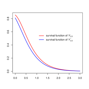
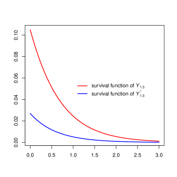
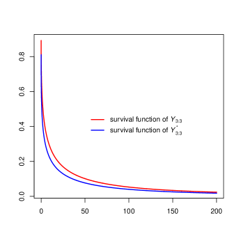
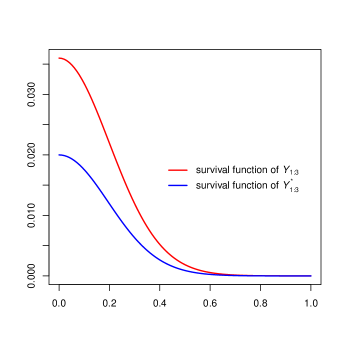
Figure 1: Plots of the survival functions of $Y_{1:3}$, $Y^{*}_{1:3}$, $Y_{3:3}$ and $Y^{*}_{3:3}$ in transmuted exponential distribution (top panels) and transmuted Weibull distribution (bottom panels).

Conclusion

In this paper, under some certain conditions, we discussed stochastic comparisons between the largest claim amounts in the sense of usual stochastic ordering and reversed hazard rate ordering and stochastic comparisons between the smallest claim amounts in the sense of usual stochastic ordering, hazard rate ordering and dispersive ordering in transmuted-G model. However, we applied some established results for two special cases of transmuted-G model, such as the transmuted exponential distribution and the transmuted Weibull distribution. It is very important to mention that the conditions of the most established results do not depend on the baseline distribution properties.

References

- (1) Al-Babtain, A. A. (2017). Transmuted Exponential Pareto Distribution with Applications. Journal of Computational and Theoretical Nanoscience, 14(11), 5484-5490.
- (2) Aryal, G.R., and Tsokos, C.P. (2011). Transmuted Weibull distribution: A generalization of the Weibull probability distribution. European Journal of Pure and Applied Mathematics, 4(2), 89-102.
- (3) Balakrishnan, N., Haidari, A. and Masoumifard, K. (2015). Stochastic comparisons of series and parallel systems with generalized exponential components. IEEE Transactions on Reliability, 64(1), 333-348.
- (4) Balakrishnan, N., Zhang, Y., and Zhao, P. (2018). Ordering the largest claim amounts and ranges from two sets of heterogeneous portfolios. Scandinavian Actuarial Journal, 2018(1), 23-41.
- (5) Barmalzan, G. and Najafabadi, A.T.P. (2015). On the convex transform and right-spread orders of smallest claim amounts. Insurance: Mathematics and Economics, 64, 380-384.
- (6) Barmalzan, G., Najafabadi, A.T.P. and Balakrishnan, N. (2015). Stochastic comparison of aggregate claim amounts between two heterogeneous portfolios and its applications. Insurance: Mathematics and Economics, 61, 235-241.
- (7) Barmalzan, G., Najafabadi, A.T.P. and Balakrishnan, N. (2016). Likelihood ratio and dispersive orders for smallest order statistics and smallest claim amounts from heterogeneous Weibull sample. Statistics and Probability Letters, 110, 1-7.
- (8) Barmalzan, G., Najafabadi, A.T.P. and Balakrishnan, N. (2017). Ordering properties of the smallest and largest claim amounts in a general scale model. Scandinavian Actuarial Journal, 2017(2), 105-124.
- (9) Bourguignon, M., Leão, J., Leiva, V., and Santos-Neto, M. (2017). The transmuted Birnbaum-Saunders distribution. REVSTAT Statistical Journal, 15, 601-628.
- (10) Denuit, M. and Frostig, E. (2006). Heterogeneity and the need for capital in the individual model. Scandinavian Actuarial Journal, 2006(1), 42-66.
- (11) Elbatal, I., and Aryal, G. (2015). Transmuted Dagum distribution with applications. Chilean Journal of Statistics, 6(12), 31-45.
- (12) Frostig, E. (2001). A comparison between homogeneous and heterogeneous portfolios. Insurance: Mathematics and Economics, 29(1), 59-71.
- (13) Granzotto, D. C. T., and Louzada, F. (2015). The transmuted log-logistic distribution: Modelling, inference, and an application to a polled tabapua race time up to first calving data. Communications in Statistics-Theory and Methods, 44(16), 3387-3402.
- (14) Hu, T. and Ruan, L. (2004). A note on multivariate stochastic comparisons of Bernoulli random variables. Journal of Statistical Planning and Inference, 126(1), 281-288.
- (15) Iriarte, Y. A., and Astorga, J. M. (2014). Transmuted Maxwell probability distribution. Revista Integración, 32(2), 211-221.
- (16) Karlin, S., and Novikoff, A. (1963). Generalized convex inequalities. Pacific Journal of Mathematics, 13(4), 1251-1279.
- (17) Kemaloglu, S. A., and Yilmaz, M. (2017). Transmuted two-parameter Lindley distribution. Communications in Statistics-Theory and Methods, 46(23), 11866-11879.
- (18) Khaledi, B.E., and Ahmadi, S.S. (2008). On stochastic comparison between aggregate claim amounts. Journal of Statistical Planning and Inference, 138(7), 3121-3129.
- (19) Khan, M.S., King, R., and Hudson, I.L. (2017). Transmuted Weibull distribution: Properties and estimation. Communications in Statistics-Theory and Methods, 46(11), 5394-5418.
- (20) Li, C. and Li, X. (2016). Sufficient conditions for ordering aggregate heterogeneous random claim amounts. Insurance: Mathematics and Economics, 70, 406-413.
- (21) Li, H. and Li, X. (2013). Stochastic Orders in Reliability and Risk. Springer, New York.
- (22) Ma, C. (2000). Convex orders for linear combinations of random variables. Journal of Statistical Planning and Inference, 84, 11-25.
- (23) Marshall, A.W., Olkin, I. and Arnold, B.C. (2011). Inequalities: Theory of Majorization and its Applications. Springer, New York.
- (24) Mirhossaini, S.M. and Dolati, A. (2008). On a New Generalization of the Exponential Distribution. Journal of Mathematical Extension, 3(1), 27-42.
- (25) Mirhossaini, S.M., Dolati, A., and Amini, M. (2011). On a class of distributions generated by stochastic mixture of the extreme order statistics of a sample of size two. Journal of Statistical Theory and Application, 10, 455-468.
- (26) Müller, A., and Stoyan, D. (2002). Comparison methods for stochastic models and risks. John Wiley & Sons, New York.
- (27) Okorie, I. E., Akpanta, A. C., and Ohakwe, J. (2016). Transmuted Erlang-truncated exponential distribution. Economic Quality Control, 31(2), 71-84.
- (28) Saboor, A., Elbatal, I., and Cordeiro, G. M. (2016). The transmuted exponentiated Weibull geometric distribution: Theory and applications. Hacettepe Journal of Mathematics and Statistics, 45, 973-987.
- (29) Shaked, M. and Shanthikumar, J.G. (2007). Stochastic Orders. Springer, New York.
- (30) Shaw, W.T. and Buckley, I.R. (2009). The alchemy of probability distributions: beyond Gram-Charlier expansions, and a skew-kurtotic-normal distribution from a rank transmutation map. arXiv preprint arXiv:0901.0434.
- (31) Tian, Y., Tian, M., and Zhu, Q. (2014). Transmuted linear exponential distribution: A new generalization of the linear exponential distribution. Communications in Statistics-Simulation and Computation, 43(10), 2661-2677.
- (32) Zhang, Y. and Zhao, P. (2015). Comparisons on aggregate risks from two sets of heterogeneous portfolios. Insurance: Mathematics and Economics, 65, 124-135.