Second-Harmonic Generation in Nano-Structured Metamaterials

Abstract

We conduct a theoretical and numerical study on the second-harmonic (SH) optical response of a nano-structured metamaterial composed of a periodic array of inclusions. Both the inclusions and their surrounding matrix are made of centrosymmetrical materials, for which SH is strongly suppressed, but by appropriately choosing the shape of the inclusions, we may produce a geometrically non-centrosymmetric system which does allow efficient SH generation. Variations in the geometrical configuration allows tuning the linear and quadratic spectra of the optical response of the system. We develop an efficient scheme for calculating the nonlinear polarization, extending a formalism for the calculation of the macroscopic dielectric function using Haydock’s recursion method. We apply the formalism developed here to an array of holes within an Ag matrix, but it can be readily applied to any metamaterial made of arbitrary materials and for inclusions of any geometry within the long-wavelength regime.

I Introduction

The advent of structured metamaterials has allowed the design of new materials, with an unprecedented amount of control over their intrinsic properties. These metamaterials are typically composite systems that consist of two or more ordinary materials, that are periodically structured or arranged in such a manner that the resulting properties differ from those of the constituent materials. These systems have been widely explored both theoretically and experimentally, with a plethora of new applications under development Veselago (1967); Garland and Tanner (1978); Smith et al. (2000, 2004); Husu et al. (2012); Larouche and Smith (2010). The variety of available fabrication techniques such as electron-beam lithography Akahane et al. (2003); Grigorenko et al. (2005); Balci et al. (2017), ion milling Gordon et al. (2004); Seniutinas et al. (2016), and even conventional 3D printing Wegener (2018); Shen et al. (2017); Mikheeva et al. (2018), allow for extremely precise designs of structured systems featuring arrays of inclusions (or holes) with specific shapes. These methods allow the fabrication of new devices with highly tunable optoelectronic properties Pendry (2000); Smith et al. (2000). A wide variety of applications using metamaterials have now been developed. Materials can be designed to have a negative index of refraction Shalaev et al. (2005); this has been implemented using periodic noble metal inclusions within a dielectric matrix Kildishev et al. (2006). Flat lens-like devices can be fabricated using metamaterials that can manipulate the propagation of light with sub-wavelength focusing capabilities; Pendry (2000) this type of device has been implemented for cloaking Pendry et al. (2006); Leonhardt (2006); Hao et al. (2010) and shielding applications Feng and Halterman (2008). The fabrication of these materials is not restricted to specific ranges of the electromagnetic spectrum, permitting, for example, the development of new devices designed to work in the terahertz regime Alekseyev et al. (2012); Born et al. (2015); Suzuki et al. (2018).

Metamaterials display a wide variety of optical phenomena Chen et al. (2010); of particular interest to us are their nonlinear optical properties. The nonlinear response is strongly sensitive to the natural atomic structure; for second-harmonic generation (SHG), the material must have a non-centrosymmetric crystalline structure in order to have a strong dipolar nonlinear response. Structured metamaterials, that can be designed with almost limitless configurations, make for a promising alternative for nonlinear optical applications. There have been numerous theoretical Larouche and Smith (2010); O’Brien et al. (2015); Larouche and Radisic (2018) and experimental Shadrivov et al. (2006); Feng and Halterman (2008); Husu et al. (2012) studies concerning the development of nonlinear devices using metamaterials. Some examples of nonlinear metamaterials have been fabricated using split-ring resonators Zharov et al. (2003); Klein et al. (2006) and nano-rod inclusions Marino et al. (2018), producing SHG-active, magnetic, and left-handed materials. Other inclusions can be intrinsically noncentrosymmetric Canfield et al. (2007), thus creating a strong SHG response. Tailored metamaterials allow for the possibility to tune the nonlinear optical response Chen et al. (2012); Timbrell et al. (2018); Bar-David and Levy (2018); Galanty et al. (2018) as a function of the geometrical configuration. These systems can be varied geometrically, changing their degree of non-centrosymmetry, thus allowing for the second-harmonic (SH) signal to be enhanced.

The required physical parameters (namely, the electric permittivity and magnetic permeability) that are used for calculating the linear optical response can be obtained via a homogenization procedure Smith et al. (2000); Simovski (2010); Alu (2011). The formalism presented in Refs. Mochán and Barrera, 1985a and Mochán and Barrera, 1985b is used in this work to describe the macroscopic linear response of inhomogeneous systems in terms of an average of certain specific microscopic response functions of the system. These quantities can then be used and the formalism may be extended to calculate the linear and non-linear optical responses of metamaterials of arbitrary composition Cortes et al. (2010); Mochán et al. (2010); Pérez-Huerta et al. (2013); Mochán et al. (2014); Mendoza and Mochán (2016). In this work, we explore the nonlinear SH response of a periodic nanostructured metamaterial comprised of an array of holes of a non-centrosymmetric geometry within a matrix made of a centrosymmeteric material, for which we chose silver. In this case, the SH generation from a homogeneous matrix would be strongly suppressed, but the noncentrosymmetric geometry of the holes allows a strong signal whose resonances may be tuned and enhanced through variations of the geometrical parametersButet et al. (2013, 2015). We systematically study the evolution of the nonlinear susceptibility tensor due to variations in the shape and position of the holes. Lastly, we elucidate the origin of the produced SH response by calculating and analyzing the charge density and polarization field at the metallic surface.

The paper is organized as follows. In Sec. II we present the theoretical approach used to calculate the dielectric response of the metamaterial that is then used to obtain the nonlinear SH polarization. In Sec. III we present results for a nanostructured metamaterial consisting of empty holes within a silver matrix. We explore a variety of geometric configurations to fine-tune the SH response. Finally, in Sec. IV we present our conclusions.

II Theory

The quadratic polarization forced at the second-harmonic (SH) frequency $2\omega$ by an inhomogeneous fundamental field $\bm{E}_{\omega}$ at frequency $\omega$ within an isotropic centrosymmetric material system made of polarizable entities within the non-retarded regime may be written as Jackson (1975)

$$\bm{P}^{f}({2\omega})=n\bm{p}({2\omega})-\frac{1}{2}\nabla\cdot n\bm{Q}({2\omega})$$ (1)

where $n$ is the number density of polarizable entities, $\bm{p}({2\omega})$ is their electric dipole moment, given within the dipolium modelMendoza and Mochán (1996) by

$$\bm{p}({2\omega})=-\frac{n}{2e}\alpha(\omega)\alpha(2\omega)\nabla E^{2}(\omega),$$ (2)

$\bm{Q}({2\omega})$ is their electric quadrupole moment, given by

$$\bm{Q}({2\omega})=\frac{1}{2e}n\alpha^{2}(\omega)\bm{E}(\omega)\bm{E}(\omega),$$ (3)

and $\alpha(\nu\omega)$ are the the linear polarizabilities of each entity at the fundamental ($\nu=1$) and at the SH ($\nu=2$), related to the dielectric function $\epsilon(\nu\omega)$ through

$$\epsilon(\nu\omega)=1+4\pi n\alpha(\nu\omega).$$ (4)

We allow the density $n$, the polarizability $\alpha$, the dielectric response $\epsilon$ and the field to depend on position. The total polarization induced at the SH is then

$$\bm{P}({2\omega})= n\alpha(2\omega)\bm{E}({2\omega})+\bm{P}^{f}({2\omega})$$

$$= n\alpha(2\omega)\bm{E}({2\omega})-\frac{n}{2e}\alpha(\omega)\alpha(2\omega)\nabla E^{2}(\omega)+\frac{1}{2e}\nabla\cdot n\alpha^{2}(\omega)\bm{E}(\omega)\bm{E}(\omega),$$ (5)

where we added to Eq. (1) the polarization linearly induced by the self-consistent electric field $\bm{E}({2\omega})$ produced by the total SH polarization $\bm{P}({2\omega})$.

We want to apply the equations above to obtain the nonlinear susceptibility of a binary metamaterial consisting of a host made up some material $A$ in which inclusions made up of a material $B$ are embeded forming a periodic lattice. In our actual calculations we will replace material B by vacuum. We denote by $\epsilon_{\gamma}$, $\alpha_{\gamma}$ and $n_{\gamma}$ the dielectric function, polarizability and number density corresponding to material $\gamma=A,$ $B$. We may describe the geometry of the metamaterial through a periodic characteristic function $B(\bm{r})=B(\bm{r}+\bm{R})$ which takes the values 1 or 0, according to whether the position $\bm{r}$ lies within the region occupied by material $B$ or $A$, respectively, and where $\bm{R}$ is a lattice vector. Thus, we may write the dielectric function as

$$\epsilon(\bm{r})=\frac{\epsilon_{A}}{u}(u-B(\bm{r})),$$ (6)

where we introduced the spectral variable

$$u=\frac{1}{1-\epsilon_{B}/\epsilon_{A}},$$ (7)

which takes complex values in general and accounts for the composition of the materials and for their frequency dependent response.

In the long wavelength approximation, assuming that the unit cell of the metamaterial is small compared to the wavelength of light in vacuum and the wave- or decay-length within each of its components, we may take the electric field within a single cell as longitudinal $\bm{E}=\bm{E}^{L}$ and we may identify the longitudinal part $\bm{D}^{L}$ of the displacement field $\bm{D}$ as an external field, which therefore has no fluctuations originated in the spatial texture of the metamaterial, and is thus a macroscopic field $\bm{D}^{L}=\bm{D}^{L}_{M}$. Thus, if we excite the system with a longitudinal external field we may write

$$\bm{E}=(\hat{\bm{\epsilon}}^{LL})^{-1}\bm{D}^{L},$$ (8)

and

$$\bm{E}_{M}=(\hat{\bm{\epsilon}}^{LL}_{M})^{-1}\bm{D}^{L}_{M},$$ (9)

where $\hat{\bm{\epsilon}}^{LL}=\hat{\mathcal{P}}^{L}\hat{\epsilon}\hat{\mathcal{P}}^{L}$ is the longitudinal projection of the dielectric function $\epsilon$ interpreted as a linear operator,

$$(\hat{\bm{\epsilon}}^{LL}_{M})^{-1}=\left\langle(\hat{\bm{\epsilon}}^{LL})^{-1}\right\rangle,$$ (10)

is the inverse of the macroscopic longitudinal dielectric operator, givenMochán and Barrera (1985a, b) by the spatial average, $\langle\ldots\rangle$, of the microscopic inverse longitudinal dielectric operator, and $\hat{\mathcal{P}}^{L}$ is the longitudinal projector operator, which may be represented in reciprocal space by the matrix

$$\mathcal{P}_{\bm{G}\bm{G}^{\prime}}=\hat{\bm{G}}\hat{\bm{G}}\delta_{\bm{G}\bm{G}^{\prime}},$$ (11)

with $\bm{G}$ and $\bm{G}^{\prime}$ reciprocal vectors of the metamaterial, where $\delta_{\bm{G}\bm{G}^{\prime}}$ is Kronecker’s delta,

$$\hat{\bm{G}}=\frac{\bm{k}+\bm{G}}{||\bm{k}+\bm{G}||}$$ (12)

a unit vector in the direction of the wavevector $\bm{k}+\bm{G}$, and $\bm{k}$ the conserved Bloch’s vector of the linear field which we interpret as the relatively small wavevector of the macroscopic field.

From Eq. (6) we may write

$$(\hat{\bm{\epsilon}}^{LL})^{-1}=\frac{u}{\epsilon_{A}}(u\hat{\mathcal{P}}^{L}-\hat{B}^{LL})^{-1},$$ (13)

in which we may interpret the inverse of the operator within parenthesis in terms of a Green’s function,

$$\hat{\mathcal{G}}(u)=(u-\hat{\mathcal{H}})^{-1},$$ (14)

the resolvent of a Hermitian operator $\hat{\mathcal{H}}$ with matrix elements

$$\mathcal{H}_{\bm{G}\bm{G}^{\prime}}=\hat{\bm{G}}\cdot B(\bm{G}-\bm{G}^{\prime})\hat{\bm{G}}^{\prime}$$ (15)

in reciprocal space, where $B(\bm{G}-\bm{G}^{\prime})$ is the Fourier coefficient of the periodic characteristic function $B(\bm{r})$ with wavevector $(\bm{G}-\bm{G}^{\prime})$. Notice that $B^{LL}_{\bm{G}\bm{G}^{\prime}}=\hat{\bm{G}}\mathcal{H}_{\bm{G}\bm{G}^{\prime}}\hat{\bm{G}}^{\prime}$, $(\bm{\epsilon}^{LL})^{-1}_{\bm{G}\bm{G}^{\prime}}=(u/\epsilon_{A})\hat{\bm{G}}\hat{\mathcal{G}}(u)\hat{\bm{G}^{\prime}}$, and that $(\bm{\epsilon}^{LL}_{M})^{-1}=(u/\epsilon_{A})\hat{\bm{k}}\langle\hat{\mathcal{G}}(u)\rangle\hat{\bm{k}}$.

To obtain the macroscopic dielectric response and the microscopic electric field we proceed as follows. We define a normalized macroscopic state $|0\rangle$ that represents a longitudinal field propagating with the given small wavevector $\bm{k}$ and we act repeatedly on this state with the operator $\hat{\mathcal{H}}$ to generate an orthonormal basis set $\{|n\rangle\}$ through Haydock’sHaydock (1980) recursion

$$\hat{\mathcal{H}}|n\rangle=b_{n+1}|n+1\rangle+a_{n}|n\rangle+b_{n}|n-1\rangle.$$ (16)

In this basis, $\hat{\mathcal{H}}$ may be represented by a tridiagonal matrix with elements

$$(\mathcal{H}_{nn^{\prime}})=\left(\begin{array}[]{ccccc}a_{0}&b_{1}&0&0&\cdots\\ b_{1}&a_{1}&b_{2}&0&\cdots\\ 0&b_{2}&a_{2}&b_{3}&\cdots\\ 0&0&b_{3}&a_{3}&\cdots\\ \vdots&\vdots&\vdots&\vdots&\ddots\end{array}\right)$$ (17)

given by Haydock’s coefficients $a_{n}$ and $b_{n}$. Thus, the macroscopic inverse longitudinal response may be obtained as a continued fraction Mochán et al. (2010); Pérez-Huerta et al. (2013)

$$\begin{split}(\hat{\bm{\epsilon}}^{LL}_{M})^{-1}&=\hat{\bm{k}}\hat{\bm{k}}\frac{u}{\epsilon_{A}}\langle 0|(u-\hat{H})^{-1}|0\rangle\\ &=\hat{\bm{k}}\hat{\bm{k}}\frac{u}{\epsilon_{A}}\frac{1}{u-a_{0}-\frac{b_{1}^{2}}{u-a_{1}-\frac{b_{2}^{2}}{u-a_{2}-\frac{b_{3}^{2}}{\ddots}}}}\end{split}$$ (18)

and the microscopic electric field (8) may be represented in reciprocal space by

$$E_{G}=\sum\zeta_{n}\langle\bm{G}|n\rangle$$ (19)

with coefficients $\zeta_{n}$ obtained by solving the tridiagonal system

$$\sum_{n^{\prime}}(u\delta_{nn^{\prime}}-H_{nn^{\prime}})\zeta_{n^{\prime}}=\delta_{n0}D^{L},$$ (20)

where we write the fields in real space as

$$\bm{D}^{L}(\bm{r})=\hat{\bm{k}}D^{L}e^{i\bm{k}\cdot\bm{r}}$$ (21)

and

$$\bm{E}(\bm{r})=\sum_{\bm{G}}\hat{\bm{G}}E_{G}e^{i(\bm{k}+\bm{G})\cdot\bm{r}}.$$ (22)

Notice that the results of the calculation above depend on the direction $\hat{\bm{k}}$ chosen as the propagation direction of the external field. As we may identify

$$(\bm{\hat{\epsilon}}_{M}^{LL})^{-1}=\frac{\hat{\bm{k}}\hat{\bm{k}}}{\hat{\bm{k}}.\bm{\hat{\epsilon}}_{M}^{LL}\cdot\hat{\bm{k}}},$$ (23)

all the components of the macroscopic dielectric tensor may be efficiently obtained from Eq. (18) by repeating the calculation of its longitudinal proyection for different propagation directions $\hat{\bm{k}}$, such as along all independent combinations $\hat{\bm{e}}_{i}+\hat{\bm{e}}_{j}$ of pairs of cartesian directions $\hat{\bm{e}}_{i}$ and $\hat{\bm{e}}_{j}$ ($i,j=x,$ $y$ or $z$).

Once we obtain the microscopic field from Eqs. (19), (20) and (22), we may substitute it in Eqs. (1)-(3) to obtain the forced SH polarization, which we may then substitute in Eq. (II) to obtain the self-consistent quadratic polarization in the SH. However, in order to solve Eq. (II) we need the self-consistent SH field, which in the long wavelength approximation is simply given by the depolarization field

$$\bm{E}({2\omega})=-4\pi\bm{P}^{L}({2\omega})$$ (24)

produced only by the longitudinal part of the SH polarization. Thus we write Eq. (II) as

$$\bm{P}({2\omega})=-4\pi n\alpha(2\omega)\bm{P}^{L}({2\omega})+\bm{P}^{f}({2\omega}).$$ (25)

By taking its longitudinal projection, we obtain a closed equation for $\bm{P}^{L}({2\omega})$ which we solve formally as

$$\bm{P}^{L}({2\omega})=(\hat{\bm{\epsilon}}^{LL}(2\omega))^{-1}\bm{P}^{fL}({2\omega})$$ (26)

using Eq. (4). Plugging this result back into Eq. (25), we finally obtain the SH polarization $\bm{P}(2\omega)$.

In order to perform the operation indicated in Eq. (26) we perform a Haydock recursion as in Eq. (16) but using $\bm{P}^{fL}{(2\omega)}$ to construct a new initial normalized state $|\tilde{0}\rangle$, with components $\langle\bm{G}|\tilde{0}\rangle$ in reciprocal given by

$$\bm{P}^{fL}_{\bm{G}}({2\omega})=\hat{\bm{G}}\langle\bm{G}|\tilde{0}\rangle f,$$ (27)

where $f$ is a normalization constant. From this state, we build a new Haydock orthonormal basis $|\tilde{n}\rangle$ using the same procedure as in Eq. (16). Thus, we write the self-consistent longitudinal SH polarization as

$$\bm{P}^{L}({2\omega};\bm{r})=\sum_{\bm{G}}P^{L}_{\bm{G}}(2\omega)\hat{\bm{G}}e^{i(\bm{k}+\bm{G})\cdot\bm{r}}.$$ (28)

with

$$P^{L}_{\bm{G}}{(2\omega)}=\frac{u_{2}}{\epsilon_{A2}}\sum_{\tilde{n}}\xi_{\tilde{n}}\langle\bm{G}|\tilde{n}\rangle$$ (29)

and with coefficients $\xi_{\tilde{n}}$ obtained by solving the tridiagonal system

$$\sum_{\tilde{n}^{\prime}}(u_{2}\delta_{\tilde{n}\tilde{n}^{\prime}}-H_{\tilde{n}\tilde{n}^{\prime}})\xi_{\tilde{n}^{\prime}}=\delta_{\tilde{n}\tilde{0}}f,$$ (30)

where $u_{2}$ and $\epsilon_{A2}$ are the spectral variable (7) and the dielectric response $\epsilon_{A}$ but evaluated at the SH frequency $2\omega$.

Substitution of $\xi_{\tilde{n}}$ from Eq. (30) into Eqs. (29) and (28) yields the SH longitudinal polarization, which may then be substituted into Eq. (25) to obtain the total SH polarization in the longwavelength limit when the system is excited by a longitudinal external field along $\hat{\bm{k}}$. Averaging the result, or equivalently, taking the $\bm{G}=0$ contribution in reciprocal space, we obtain the macroscopic SH polarization $\bm{P}_{M}(2\omega)$ which we write as

$$\bm{P}_{M}({2\omega})=\frac{1}{4\pi}(\bm{\epsilon}_{M}(2\omega)-\bm{1})\bm{E}_{M}({2\omega})+\bm{P}_{M}^{f}({2\omega}),$$ (31)

where the first term is the contribution of the linear response at $2\omega$ to the SH macroscopic field, and the second term

$$\bm{P}_{M}^{f}({2\omega})=\bm{\chi}^{(2)}_{M}:\bm{E}_{M}({\omega})\bm{E}_{M}({\omega})$$ (32)

is the sought after contribution to the SH macroscopic polarization forced by the fundamental macroscopic electric field, and $\bm{\chi}^{(2)}_{M}$ is the corresponding SH quadratic macroscopic susceptibility, given by a third rank tensor. Within our longwavelength longitudinal calculation the macroscopic field $\bm{E}_{M}({2\omega})$ is simply given by the longitudinal depolarization field

$$\bm{E}_{M}({2\omega})=\bm{E}^{L}_{M}({2\omega})=-4\pi\bm{P}^{L}_{M}({2\omega}),$$ (33)

so that, taking the longitudinal projection of Eq. (31) we obtain

$$\bm{P}_{M}^{fL}({2\omega})=\hat{\bm{k}}\hat{\bm{k}}\cdot\bm{P}_{M}^{f}({2\omega})=\bm{\epsilon}_{M}^{LL}(2\omega)\bm{P}_{M}^{L}({2\omega}).$$ (34)

Substituting $\bm{P}_{M}^{fL}({2\omega})$ from Eq. (34) into (33) and then into (31) we obtain the macroscopic forced quadratic SH polarization $\bm{P}_{M}^{f}(2\omega)$ produced by a longitudinal external $\bm{D}^{L}$ field pointing along $\hat{\bm{k}}$. As in the linear case, we finally repeat the calculation above, for several independent directions of propagation $\hat{\bm{k}}$ so that the corresponding Eqs. (32) become a system of linear equations in the unknown cartesian components $\chi^{(2)}_{M\,ijk}$ ($i,j,k=x,$ $y,$ or $z$) which we solve to obtain the third rank second order susceptibility tensor $\bm{\chi}^{(2)}_{M}$ of the metamaterial.

In summary, to obtain the quadratic response we first obtain the nonretarded microscopic field and the macroscopic dielectric tensor using a Haydock’s recursion starting from a macroscopic external longitudinal field, then we use the dipolium model to obtain the microscopic source of the SH polarization, we screen it using Haydock’s scheme again to obtain the full microscopic polarization, which we average to obtain the full macroscopic SH polarization. As this includes a contribution from the macroscopic SH depolarization field, we substract it before identifying the quadratic suceptibility tensor projected onto the longitudinal direction. We repeat the calculation along different independent directions so that we can extract all the components of the quadratic susceptibility.

In the process above we assumed that the unit cell of the metamaterial is small with respect to the wavelength at frequency $\omega$, and thus we introduced a long-wavelength approximation and assumed the external field and the electric field to be longitudinal. After obtaining all the components of the macroscopic response, we should not concern ourselves anymore with the texture of the metamaterial; the unit cell disappears from any further use we give to the macroscopic susceptibility. Thus, we can solve any macroscopic SH related electromagnetic problem using the suceptibility obtained above without using again the long wavelength approximation. Once we have the full macroscopic susceptibility tensor we may use it to calculate the response to transverse as well as longitudinal fields. Thus, we may use our susceptibility above to study the generation of electromagnetic waves at the SH from a propagating fundamental wave, in which case the macroscopic fields can no longer be assumed to be longitudinal.

III Results

We present results for a simple geometry in which we can control the degree of centrosymmetry. To that end, we incorporated the scheme described in the previous section into the package Photonic pho (2018), which is a modular, object oriented system based on the Perl programming language, its Perl Data Language (PDL) Glazebrook and Economou (1997) extension for efficient numerical calculations, and the Moose Ducasse et al. (2000) object system. The package implements Haydock’s recursive procedure to calculate optical properties of structured metamaterials in the nonretarded as well as in the retarded regime.

Our system consists of a square array of pairs of holes in the shape of prisms with a rectangular cross section within a metallic host (Fig. 1).

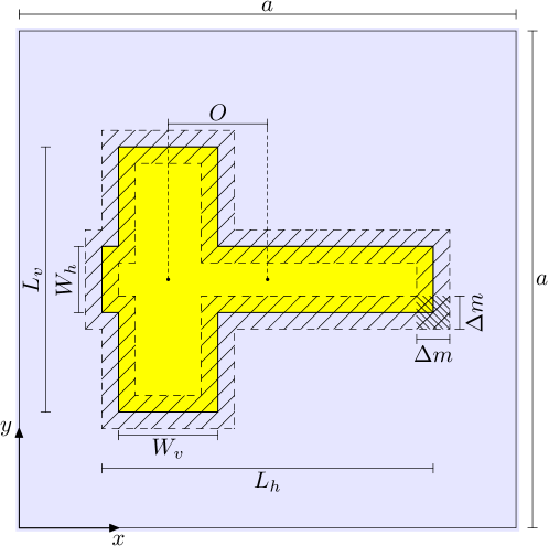
Figure 1: Unit cell of a metamaterial made up of a horizontal and a vertical rectangular hole within a conducting matrix. We indicate the lattice parameter $a$ of the square array, the length $L_{\beta}$ and width $W_{\beta}$ of each rectangle ($\beta=h,v$) and the offset $O$ of the center of the vertical rectangle with respect to that of the horizontal one. We indicate the directions $x$, $y$ of the crystalline axes. The shaded regions correspond to masks of width $\Delta m$ used to single out the surface, edge and corner contributions to the SH response.

Each rectangle is aligned with one of the crystalline axes $x$, $y$ of the metamaterial and is characterized by its length $L_{h}$ or $L_{v}$ and its width $W_{h}$ or $W_{v}$, where $h$ denotes horizontal (along $x$) and $v$ vertical (along $y$) alignment. The center of the vertical rectangle is shifted horizontally with respect to the center of the horizontal rectangle by an offset $O$. Thus, when $O=0$ our system is centrosymmetric and as $O$ increases it becomes noncentrosymmetric in varying degrees.

In order to simplify our analysis, we have chosen a system that has mirror symmetry $y\leftrightarrow-y$. Thus, the only in-plane non-null components of the SH susceptibility arePopov (2017) $\chi_{xxx}$, $\chi_{xyy}$, and $\chi_{yxy}=\chi_{yyx}$. We omit the subindex $M$ and the superindex $(2)$ that indicate these are components of the quadratic macroscopic susceptibility in order to simplify the notation, as we expect it yields no confusion. In Fig. 2 we show the spectra of the magnitude of these non-null components for an Ag hostYang et al. (2015) and for different values of the offset $O$. The parameters we used were $W_{h}=W_{v}=a/6$, $L_{h}=L_{v}=a/2$, $O=0\ldots a/3$.

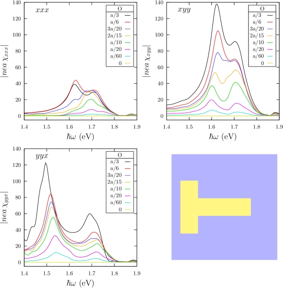
Figure 2: Normalized absolute value of the non-null components of the SH susceptiblity $nea\chi_{ijk}$, with $ijk=xxx$ (upper left), $xyy$ (upper right), and $yyx=yxy$ (lower left), for a square lattice of rectangular holes, as in Fig. 1 within an Ag matrix, with geometrical parameters $L_{h}=L_{v}=a/2$, $W_{h}=W_{v}=a/6$, for different values of the offset $O=0\ldots a/3$. The lower right panel displays the geometry corresponding to the largest offset. Notice that for these cases the holes overlap.

Notice that when $O=0$ the system is centrosymmetric and there is no SH signal. As $O$ increases towards $\pm a/3$ the system becomes noncentrosymmetric. Two resonances become clearly visible and they grow in size as $O$ increases and the system moves farther away from the centrosymmetric case. The lower energy resonance of $\chi_{yyx}$ is at a different frequency than those of $\chi_{xxx}$ and $\chi_{xyy}$ and is red shifted as the offset increases. If $O$ increases beyond $a/3$ (not shown) the two rectangles would cease to overlap and the quadratic suceptibility would rapidly decay, until $O=a/2$ for which the system becomes exactly centrosymmetric again and the quadratic susceptibility becomes exactly null.

According to Fig. 2, the order of magnitude of the SH susceptibility is around $10^{2}/nea$. For typical noncentrosymmetrical materials, such as quartz, the corresponding order of magnitude is about $1/nea_{B}$, where $a_{B}$ is Bohr radiusBoyd (2003). Thus, a centrosymmetric material with a noncentrosymmetric geometry can achieve susceptibilities of the order of $10^{2}a_{B}/a$ times that of noncentrosymmetrical materials. Thus, quadratic metamateriales made of centrosymmetrical materials may be competitive as long as the lattice parameter is not too large.

In order to understand the origin of the structure of the spectra discussed above, in Fig. 3 we plot the non-null components $\epsilon_{M}^{xx}$ and $\epsilon_{M}^{yy}$ of the macroscopic linear dielectric tensor $\bm{\epsilon}_{M}$ of a metamaterial made up of a square lattice of single rectangular holes with a horizontal orientation. Notice that there is a very weak resonance close to 3.4 eV corresponding to polarization along the length of the rectangle ($x$ direction) and a strong resonance corresponding to polarization along the width of the rectangle ($y$ direction) at a slightly smaller frequency.

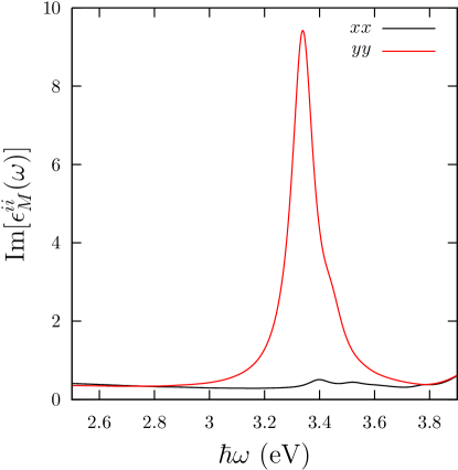
Figure 3: Non-null components of the macroscopic dielectric response, $\epsilon_{M}^{xx}$ and $\epsilon_{M}^{yy}$, of a metamaterial made up of a square array of horizontally oriented single rectangular holes with the same dimensions as in Fig. 2 within an Ag matrix.

Although there is a strong linear resonance in the $y$ direction, this system is centrosymmetrical and would yield no SH signal. When we combine horizontal and vertical rectangles (Fig. 4) with a null offset $O=0$ to make a centrosymmetric array of crosses, both resonances appear for both polarizations, although they now interact, partially exchange their strengths and repel so that both become clearly visible close to 3.4 eV and 3.2 eV.

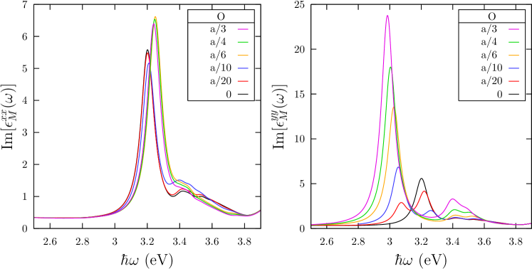
Figure 4: Non-null components $\epsilon_{M}^{xx}$ and $\epsilon_{M}^{yy}$ of the macroscopic dielectric tensor $\bm{\epsilon}_{M}$ of a metamaterial made up of a square lattice of pairs of horizontally and vertically oriented single rectangular holes within an Ag matrix as in Fig. 1 with the same parameters as in Fig. 2 for different values of the offset $O=0\ldots a/3$.

As the offset $O$ increases, there are only small changes to the spectra corresponding to $\epsilon_{M}^{xx}$, consisting in changes to the weights of the peaks. However, a new strong mode develops in the spectra of $\epsilon_{M}^{yy}$. This mode is due to the strong coupling of a quadrupolar oscillation in the vertical rectangle to the vertical dipolar oscillation of the horizontal rectangle. This quadrupole may be visualized as a horizontal polarization in the upper part of the vertical rectangle and a horizontal polarization in the opposite direction in the lower part of the rectangle, as illustrated by Fig. 5. The coupling is symmetry allowed as for a finite offset $O\neq 0$ the system looses the $x\leftrightarrow-x$ symmetry.

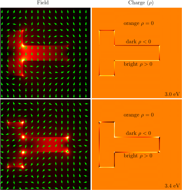
Figure 5: Magnitude (color coded) and direction (arrows) of the microscopic linear electric field (left) and induced charge density $\rho$ (right) for a metamaterial made of a square lattice of rectangular holes within an Ag matrix with the same parameters as in Fig. 2 with an offset $O=a/3$, excited by a macroscopic field along the $y$ (vertical) direction for $\hbar\omega\approx 3\,eV$ and $\hbar\omega\approx 3.4\,eV$ corresponding to the two peaks in $\epsilon_{M}^{yy}$ shown in Fig. 4. The field and the charge distribution correspond to a vertical polarization for the horizontal rectangle, a vertical polarization for the vertical rectangle and a nondiagonal quadrupole with opposite horizontal polarizations above and below the symmetry plane.

We expect the resonant structure of the quadratic susceptibility to have peaks corresponding to the resonances of the linear response at the fundamental and at the SH frequency. Thus, we expect peaks at the fundamental and at the subharmonics of those of the linear response. As there is no structure in the linear response within the region from 1.4 eV to 1.9 eV shown in Fig. 2, in our system we can only expect structure at the subharmonics, due to a resonant excitation of the polarization at the SH frequency. For a macroscopic field oriented along the cartesian directions $x$ or $y$ the SH harmonic polarization can only point along the $x$ direction, due to the $y\leftrightarrow-y$ mirror symmetry of our system. Thus, the subharmonics of the resonances of $\epsilon_{M}^{xx}$ (Fig. 4) appear in the susceptibility components $\chi_{xxx}$ and $\chi_{xyy}$ (Fig. 2). On the other hand, a macroscopic field that points along an intermediate direction between $x$ and $y$ may excite a quadratic polarization along $y$. Thus, the subharmonics of the resonances of $\epsilon_{M}^{yy}$ (Fig. 4) appear in the susceptibility components $\chi^{yxy}=\chi^{yyx}$ (Fig. 2).

To gain further insight into the nature of the resonances, in Fig. 6 we show the polarization maps evaluated at the maxima of the SH spectra corresponding to different directions of the macroscopic linear field, and for the offset $O=a/3$ that yields the largest signals.

Figure 6: Magnitude and direction of the quadratic polarization induced in the same system as in Fig. 2 for the largest offset $O=a/3$ at the resonant energies $\hbar\omega=1.62\,eV$ and the fundamental macroscopic field $\bm{E}_{M}$ along the direccion $\hat{x}$ (upper left), $\hbar\omega=1.62\,eV$ and $\bm{E}_{M}$ along $y$ (upper right) and for $\hbar\omega=1.5\,eV$ and $\hbar\omega=1.72\,eV$ with $\bm{E}_{M}$ along $\hat{x}+\hat{y}$ (bottom).

We notice that when the fundamental macroscopic field points along the $x$ or along the $y$ direction, the magnitude of the SH polarization is symmetric with respect to the mirror plane, the $y$ component of the polarization points towards opposite directions on either side of the mirror plane, yielding a macroscopic SH polarization along $x$. In these cases, the polarization has maxima near the four concave vertices of the vertical hole and near the convex vertex where the horizontal and vertical rectangles meet. On the other hand, when the fundamental macroscopic field points along the direction of $\hat{x}+\hat{y}$, the resulting quadratic polarization has no symmetry at all, and it yields a macroscopic SH polarization that has a $y$ component.

Finally, in Fig. 7 we illustrate the contributions of the surface region to the total quadratic susceptibility by adding only the contributions within bands of varying widths $\Delta m$ around the surface.

Figure 7: Contributions to the quadratic susceptibility $\chi_{xyy}$ of the same system as in Fig. 6 from the region within a distance $\Delta m$ from the surface, as defined in Fig. 1 for various values of $\Delta m=a/120,a/60,a/12$, and the full susceptibility.

We notice that although there is a very strong surface polarization, its contribution to the macroscopic quadratic susceptibility is relatively small, as it is confined to a very narrow region and it is partially cancelled by the polarization at other parts of the surface, so that for the geometry studied here, most of the SH signal comes from the bulk of the host.

IV Conclusions

We have developed a formalism for the calculation of the second order susceptibility of structured binary metamaterials formed by a lattice of particles embedded within a host, for the case where both components consists of centrosymmetric materials but where the geometry is not centrosymmetric. Although SH is strongly suppressed within a homogeneous centrosymmetric material, the noncentrosymmetric surface is capable of sustaining a surface nonlinear polarization and to induce a strongly varying linear field which induces a multipolar nonlinear polarization within the metamaterial components.

We implemented our formalism using the Haydock recursive scheme within the Photonic modular package and applied it to the calculation of the second-order nonlinear susceptibility of a structured metamaterial composed of a homogeneous Ag host with a lattice of pairs of rectangular holes. By modifying the geometry of the holes, we modify the degree of non-centrosymmetry of the material, allowing us to fine-tune both the peak position and intensity of the SH response. The SH signal is very sensitive to changes in the geometrical parameters of the structure.

After establishing the inclusion shape that most enhances this signal, we analyzed the polarization field and showed that the SH response is largest at resonance close to the concave and convex corners but it extends well into the host material. The order of magnitude of the susceptibility obtained in this calculation is comparable to that of typical non-centrosymmetric materials.

Although this study was carried out for one particular combination of materials, the employed procedure is equally valid for calculating the nonlinear properties for any metamaterial composed of arbitrary materials and inclusions. Only a priori knowledge of the dielectric function of each constituent material is required. This approach affords the opportunity to quickly and efficiently study a limitless range of possible metamaterial designs, with manifold optical applications in mind. Our hope is that this methodology will prove to be an important tool for future metamaterial design and fabrication.