Nucleon in a periodic magnetic field: finite-volume aspects

Abstract

The paper presents an extension and a refinement of our previous work on the extraction of the doubly virtual forward Compton scattering amplitude on the lattice by using the background field technique Agadjanov:2016cjc . The zero frequency limit for the periodic background field is discussed, in which the well-known result is reproduced. Further, an upper limit for the magnitude of the external field is established for which the perturbative treatment is still possible. Finally, the framework is set for the evaluation of the finite-volume corrections allowing for the analysis of upcoming lattice results.

I Introduction

Using the background field technique on the lattice for the extraction of various hadronic observables has proven to be extremely efficient. As examples we mention the measurement of magnetic moments, polarizabilities and axial-vector matrix elements of baryons and light nuclei in constant background fields Savage:2016kon ; Chang:2015qxa ; Beane:2014ora ; Beane:2015yha ; Chambers:2015bka ; Chambers:2014qaa ; Chang:2015qxa . Moreover, non-uniform background fields have been used for the calculation of the hadronic vacuum polarization tensor, hadronic form-factors and the nucleon structure functions, as the fields, which are periodic in space, allow one to measure current matrix elements at a given non-zero three-momentum transfer Bali:2015msa ; Chambers:2017tuf ; Chambers:2017dov . Different scenarios for implementing periodic background fields in lattice QCD calculations are considered in Ref. Davoudi:2015cba .

In Ref. Agadjanov:2016cjc we described a framework, based on the background field method, which enables one to extract the doubly-virtual forward Compton scattering amplitude from lattice QCD calculations (note that later, in Ref. Chambers:2017dov , a very similar formula was given without a derivation, see Eq. (12) in that paper). Low-energy Compton scattering plays an indispensable role in probing the electromagnetic structure of hadrons (for recent work, see Ref. Hagelstein:2015egb ). For example, it enters the expression for the proton-neutron electromagnetic mass difference Cottingham:1963zz , as well as the expression for the Lamb shift of the muonic hydrogen, which is used to extract the value of the proton radius (see, e.g. Ref. Carlson:2011zd ). In this paper, we in particular focus on the relevant spin-independent invariant amplitudes, denoted as $T_{1}$ and $T_{2}$, respectively. The experimental data on the structure functions completely determine the amplitude $T_{2}$ through dispersion relations. The fixed-$q^{2}$ dispersion relation for the amplitude $T_{1}$, however, requires a subtraction. Thus, the subtraction function $S_{1}(q^{2})\equiv T_{1}(0,q^{2})$ remains the only input in the calculations, which is not fixed by experimental data. Its elastic part is essentially given by the Born terms, but the inelastic piece is known only at the real photon point $q^{2}=0$ (the low-energy theorem, see, e.g., Ref. Gasser:2015dwa ).

In the past, there have been attempts to model the subtraction function, using phenomenological parameterizations WalkerLoud:2012bg ; Erben:2014hza ; Cushman:2018zza . However, this type of approach inherently contains a systematic error, which is very hard to control. Further, the subtraction function can be extracted from the Compton scattering amplitude, calculated in the low-energy EFT of QCD Bernard:2002pw ; Peset:2014jxa ; Bernard:2012hb . However, here the difficult question about the convergence of the chiral expansion arises, namely, up to which value of $q^{2}$ the results of the chiral expansion can be trusted. Recently, the authors of Ref. Gasser:2015dwa have been able to determine the subtraction function by invoking the so-called Reggeon dominance hypothesis, considered first in Ref. Gasser:1974wd . In particular, it is assumed that the forward Compton scattering amplitude does not contain any fixed pole. In Regge theory, such a pole generates an energy-independent contribution to the amplitude (such as, e.g., local two-photon couplings in scalar QED). If the fixed poles are present, the subtraction function, in general, deviates from the predicted one. In some cases, e.g., the $q^{2}$-independent fixed pole Brodsky:2008qu , the behavior of the $S_{1}(q^{2})$ can be also predicted (see Ref. Gorchtein:2013yga ), and is different from the one calculated in the absence of the fixed pole.

Hence, lattice QCD provides a model-independent approach to the verification of the Reggeon dominance hypothesis. The question whether there is a fixed pole in the Compton scattering is of conceptual interest and is still open.

In Ref. Agadjanov:2016cjc , we considered the case of a nucleon placed in a static periodic magnetic field ${\bf B}=(0,0,B^{3})$ with $B^{3}=-B\cos(\boldsymbol{\omega}{\bf x})$ and $\boldsymbol{\omega}=(0,\omega,0)$. It has been shown that, for $\omega\neq 0$, the measurement of the spin-averaged energy shift of the nucleon in this field allows one to extract the value of the subtraction function $S_{1}(-\boldsymbol{\omega}^{2})$ at non-zero values of $q^{2}=-\boldsymbol{\omega}^{2}$. The relation between these two quantities takes the form:

$$\delta E=\frac{(eB)^{2}}{4m}\,S_{1}(-\boldsymbol{\omega}^{2})\,.$$ (1)

Here, $\delta E$ denotes the spin-averaged energy shift, and $m$ stands for the nucleon mass.

The result, obtained in Ref. Agadjanov:2016cjc , still leaves room for improvement. In particular, one should find the answer to the following questions:

• In the limit $\omega\to 0$, we arrive at the case of a constant magnetic field. This case is studied very well, both analytically and numerically. However, our expressions become singular in this limit, contradicting the expectations. One needs to understand how this limit can be approached smoothly.

• Our approach relies on a perturbative expansion of the energy shift $\delta E$ in the external field strength $B$. What is the radius of the convergence of this expansion? Note that, for example, in the zero-frequency limit $\omega\to 0$, the radius is equal to zero in case of a charged particle, since the Landau levels are formed for any value of $B$. In Ref. Agadjanov:2016cjc , using heuristic arguments, for a given value of $\omega$, we gave a very rough estimate of the maximal value of $B$, for which the perturbative expansion should still work. These arguments should be refined in order to obtain a more reliable result.

• Our expressions were obtained in the infinite-volume limit. The issue of the finite-volume corrections in the presence of the external fields is a rather subtle one, since gauge-invariant non-local objects (Wilson lines) can be formed in a finite volume. For this reason, it is mandatory to re-formulate the problem in a finite volume from the beginning and to give a consistent interpretation of the finite-volume result it terms of the subtraction function, defined in the infinite volume.

The aim of the present paper is to answer the questions given above. The plan of the paper is as follows. In section II we give a collection of basic definitions and discuss two different implementations of the external field on the lattice. In sections III and IV, we give two alternative derivations of the energy shift formula in the periodic external field, based on the matching to the non-relativistic EFT, as well as the direct derivation within the relativistic framework. Both settings are complementary to each other. For example, the first derivation is more intuitive and uses ordinary quantum-mechanical Rayleigh-Schrödinger perturbation theory for the energy levels. In particular, the zero-frequency limit $\omega\to 0$ as well as the issues related to the convergence of the perturbative expansion can be considered more easily in this formulation. By contrast, the relativistic formulation allows one to investigate the exponentially suppressed finite-volume corrections in a direct manner. For completeness, in the appendix we give yet another derivation of the expression for the energy shift, considering the behavior of the nucleon two-point function at large time separations.

II Definitions and setup

II.1 Basic definitions

The matrix element of the electromagnetic current between one-nucleon states is given by

$$\langle p^{\prime},s^{\prime}|j^{\mu}(0)|p,s\rangle=\bar{u}(p^{\prime},s^{\prime})\Big{\{}\gamma^{\mu}F_{1}(q^{2})+i\sigma^{\mu\nu}F_{2}(q^{2})\frac{q_{\nu}}{2m}\Big{\}}u(p,s)\,.$$ (2)

Here, $j^{\mu}(x)$ is the electromagnetic current, and $q=p^{\prime}-p$, and $p\,(p^{\prime})$ and $s\,(s^{\prime})$ are the four-momenta and spin projections of the initial (final) nucleon, respectively. Further, $F_{1}$ and $F_{2}$ denote the Dirac and Pauli form factors. The Sachs form factors are defined by

$$G_{E}(q^{2})=F_{1}(q^{2})+\frac{q^{2}}{4m^{2}}F_{2}(q^{2})\,,\quad\quad G_{M}(q^{2})=F_{1}(q^{2})+F_{2}(q^{2})\,.$$ (3)

The Dirac spinors are normalized as $\bar{u}(p,s^{\prime})u(p,s)=2m\delta_{s^{\prime}s}$.

The Compton tensor is defined as:

$$T^{\mu\nu}(p^{\prime},s^{\prime};p,s;q)=\frac{i}{2}\int d^{4}xe^{iq\cdot x}\langle p^{\prime},s^{\prime}|Tj^{\mu}(x)j^{\nu}(0)|p,s\rangle,$$ (4)

where $q$ is the photon momentum. Taking into account Lorentz invariance, current as well as parity conservation, one arrives at the well-known decomposition of the matrix element in Eq. (4) in terms of Tarrach’s amplitudes Tarrach ; Bernabeu:1976jq . For our purposes, it is sufficient to consider the process in the forward direction $p^{\prime}=p$ and perform spin-averaging in Eq. (4):

$$T^{\mu\nu}(p,q)=\frac{1}{2}\sum_{s}T^{\mu\nu}(p,s;p,s;q).$$ (5)

The tensor $T^{\mu\nu}(p,q)$ is related to the aforementioned invariant amplitudes $T_{1},\,T_{2}$ through the decomposition (see, e.g., Ref. Gasser:2015dwa ):

$$T^{\mu\nu}(p,q)=T_{1}(\nu,q^{2})K_{1}^{\mu\nu}+T_{2}(\nu,q^{2})K_{2}^{\mu\nu},$$ (6)

where the kinematic structures $K_{1}^{\mu\nu},\,K_{2}^{\mu\nu}$ read

$$K_{1}^{\mu\nu} =q^{\mu}q^{\nu}-g^{\mu\nu}q^{2},$$

$$K_{2}^{\mu\nu} =\frac{1}{m^{2}}\Big{\{}(p^{\mu}q^{\nu}+p^{\nu}q^{\mu})p\cdot q-g^{\mu\nu}(p\cdot q)^{2}-p^{\mu}p^{\nu}q^{2}\Big{\}}.$$ (7)

Here, $\nu\equiv p\cdot q/m$.

According to the asymptotic behavior of the structure functions at large values of the parameter $\nu$, the dispersion relation for the amplitude $T_{1}(\nu,q^{2})$ requires one subtraction. It is usually performed at $\nu=0$, and hence the subtraction function $S_{1}$ is defined as

$$S_{1}(q^{2})=T_{1}(0,q^{2})\,.$$ (8)

The function $S_{1}(q^{2})$ can be formally split in two parts:

$$S_{1}(q^{2})=S_{1}^{\rm el}(q^{2})+S_{1}^{\rm inel}(q^{2})\,.$$ (9)

The elastic term $S_{1}^{\rm el}(q^{2})$ is associated with the one-nucleon exchange in the $s$- and $u$-channels. The inelastic piece $S_{1}^{\rm inel}(q^{2})$ is a regular function of $q^{2}$. We use the same definition of the elastic part as in Ref. Agadjanov:2016cjc :

$$S^{\rm el}_{1}(q^{2})=-\frac{4m^{2}}{q^{2}(4m^{2}-q^{2})}(G_{E}^{2}(q^{2})-G_{M}^{2}(q^{2}))\,.$$ (10)

Little information is available on the inelastic part of the subtraction function $S_{1}^{\rm inel}(q^{2})$. According to the low-energy theorem, its value at $q^{2}=0$ is given by

$$S_{1}^{\rm inel}(0)=-\frac{\kappa^{2}}{4m^{2}}-\frac{m}{\alpha}\,\beta_{M}\,.$$ (11)

Here, $\beta_{M}$ denotes the magnetic polarizability of the nucleon, $\alpha\simeq 1/137$ is the fine structure constant and $\kappa=F_{2}(0)$ is the anomalous magnetic moment of the nucleon. At large values of $q^{2}$, the asymptotic behavior of the subtraction function is fixed by the operator product expansion (see, e.g., Ref. Erben:2014hza ; Hill:2016bjv ). Otherwise, it is unknown in the intermediate kinematic region $0<-q^{2}\lesssim$ 2 GeV², which is amenable to lattice simulations.

II.2 External field configuration

In Ref. Agadjanov:2016cjc , it was proposed to place the nucleon in the time-independent periodic magnetic field

$${\bf B}=(0,0,B^{3}),\quad B^{3}=-eB\cos(\omega x^{2})\,,$$ (12)

where $B$ denotes the strength of the field and the frequency $\omega$ takes nonzero values. The components of the gauge field $A^{\mu}(x)$ are chosen as follows:

$$A^{1}=\frac{eB}{\omega}\sin(\omega x^{2}),\qquad A^{0}=A^{2}=A^{3}=0\,.$$ (13)

The magnetic flux is quantized in a finite box of size $L$:

$$\int_{-L/2}^{L/2}dx^{1}dx^{2}B^{3}(x^{2})=6\pi N\,,$$ (14)

As discussed in Ref. Davoudi:2015cba , this quantization condition can be implemented on the lattice in two different ways. In the first scenario, the frequency $\omega$ is constrained and no constraint is imposed on the magnetic field strength $B$. In the second scenario, the situation is reversed. Hence, we have:

a) $$\qquad\omega=\frac{2\pi n}{L},\qquad n\in\mathbb{Z}\backslash\{0\},\quad{\rm arbitrary}\,\,B,$$ (15)

b) $$\qquad B=\frac{6\pi N}{eL^{2}}\frac{\omega L/2}{\sin(\omega L/2)},\qquad N\in\mathbb{Z}\backslash\{0\},\quad{\rm arbitrary}\,\,\omega\neq\frac{2\pi n}{L}\,.$$ (16)

Only the first scenario was considered in Ref. Agadjanov:2016cjc . In the present paper, we will exploit both quantization possibilities and demonstrate that the obtained results are quite different. Obviously, the limit $\omega\to 0$ can be directly performed in the second setting only, where $\omega$ is a free parameter, unrelated to the box size $L$.

III Non-relativistic framework

III.1 Method

The framework, which is based on the use of the non-relativistic EFT, consists of two steps. At the first stage, one matches the parameters of the non-relativistic Lagrangian to the expression of the relativistic two-point function of the nucleon in an external field. At the next step, one uses the resulting non-relativistic Hamiltonian to carry out the calculation of the spectrum. The advantage of the method is its transparency: the calculations of the spectrum are done by using ordinary perturbation theory in quantum mechanics. The setting is, however, not well suited for the calculation of the finite-volume corrections, which are proportional to $\exp(-M_{\pi}L)$ where $M_{\pi}$ denotes the pion mass. Within this approach, these corrections should be included in the couplings of the non-relativistic Lagrangian through the matching procedure.

Let us consider the two-point function of the nucleon, placed in the external field $A^{\mu}(x)$. The path integral representation in Minkowski space reads:

$$\left\langle 0|T\Psi(x)\bar{\Psi}(y)|0\right\rangle_{A}=\frac{\displaystyle\int{\cal D}G{\cal D}q{\cal D}\bar{q}\,\Psi(x)\bar{\Psi}(y)e^{i\int d^{4}x({\cal L}+A_{\mu}(x)j^{\mu}(x))}}{\displaystyle\int{\cal D}G{\cal D}q{\cal D}\bar{q}\,e^{i\int d^{4}x({\cal L}+A_{\mu}(x)j^{\mu}(x))}},$$ (17)

where the integration over all possible gluon, quark and antiquark field configurations is performed. Further, $j_{\mu}(x)$ is the electromagnetic current, built of the quark fields, and $\Psi(x)$ denotes the composite nucleon field operator in QCD. Expanding the right-hand-side of Eq. (17) up-to-and-including $O(A^{2})$, one obtains

$$\langle 0|T\Psi(x)\bar{\Psi}(y)|0\rangle_{A} = \langle 0|T\Psi(x)\bar{\Psi}(y)|0\rangle_{0}+\frac{i}{1!}\int d^{4}zA_{\mu}(z)\langle 0|T\Psi(x)\bar{\Psi}(y)j^{\mu}(z)|0\rangle_{0}$$ (18)

$$+ \frac{i^{2}}{2!}\int d^{4}z_{1}d^{4}z_{2}A_{\mu}(z_{1})A_{\nu}(z_{2})\langle 0|T\Psi(x)\bar{\Psi}(y)j^{\mu}(z_{1})j^{\nu}(z_{2})|0\rangle_{0}+\cdots\,,$$

where the subscript “0” refers to the quantities evaluated in QCD without any external field, and we have used the fact that $\left\langle 0|j^{\mu}(x)|0\right\rangle_{0}=0$. Note that the expansion in Eq. (18) is written down for connected matrix elements (the subscript “conn” is omitted everywhere for brevity).

In the above quantities, the nucleons are in general off the mass shell. Performing the Fourier transform in Eq. (18), amputating the external nucleon legs, and putting the external nucleons on the mass shell, we see that the nucleon electromagnetic vertex $\langle p^{\prime},s^{\prime}|j^{\mu}(0)|p,s\rangle$ emerges at order $A$. At order $A^{2}$, the Compton tensor, defined in Eq. (4), is obtained from the matrix element $\langle 0|T\Psi(x)\bar{\Psi}(y)j^{\mu}(z_{1})j^{\nu}(z_{2})|0\rangle_{0}$. Note that, in general, the described procedure is equivalent to replacing the nucleon fields $\Psi(x)$ and $\bar{\Psi}(y)$ by the out- and ingoing nucleon states, $\langle p^{\prime},s^{\prime}|$ and $|p,s\rangle$ respectively. This fixes the overall normalization of the quantity we are considering below.

III.2 Matching

The first few terms of the effective Lagrangian, which describe the interaction of the nucleon with an external electromagnetic field, are given by:

$${\cal L}_{\rm eff}=\psi^{\dagger}\biggl{(}iD_{t}-m+\frac{{\bf D}^{2}}{2m}+\cdots\biggr{)}\psi-\frac{\mu}{e}\,\psi^{\dagger}\boldsymbol{\sigma}\cdot\mathbf{B}\psi+\frac{2\pi}{e^{2}}\,\psi^{\dagger}({\alpha}_{E}\mathbf{E}^{2}+{\beta}_{M}\mathbf{B}^{2})\psi+\cdots,$$ (19)

where the ellipses denote higher order terms with derivatives,

$$D_{t}=\partial_{t}-igA^{0}\,,\quad\mathbf{D}=\nabla+ig\mathbf{A}\,.$$ (20)

Here, $\psi(x)$ denotes the two-component nucleon field, $\mu$ is the magnetic moment and $\alpha_{E},\beta_{M}$ are the electric and magnetic polarizabilities, respectively. The coupling constant $g$ takes the values $g=0,+1$ for the neutron and proton, respectively, and ${\bf E},{\bf B}$ are the electric and magnetic fields (in order to simplify the notations, we include the factor $e$ in the definition of the vector-potential $A^{\mu}$). The NRQED Lagrangian at order $m^{-4}$ is given, e.g., in Ref. Hill:2012rh .

If the properties of a nucleon at rest are calculated, it suffices to write down only the first few terms in the Lagrangian. However, we are studying the nucleon in a periodic field, with $\omega$ corresponding to the magnitude of the momentum transfer from the field to the nucleon. Consequently, we have to retain all terms in the derivative expansion of the Lagrangian given by Eq. (19). In this case, the exact relativistic dispersion relation for the energy of the free nucleon with the three-momentum $\mathbf{p}$, $w(\mathbf{p})=\sqrt{m^{2}+\mathbf{p}^{2}}$, is satisfied.

An important remark is in order. In the infinite volume, one is allowed to use partial integration in the Lagrangian. The same is true in a finite volume, if all fields (including the external electromagnetic field) are subject to periodic boundary conditions, since the surface terms vanish in this case. The above remark will be relevant, if the realization of the external field is carried out according to the scenario b) from section II.2: the Lagrangians, which differ only by surface terms and lead to the same amplitudes in the matching condition, might yield a different spectrum in the finite volume. Bearing this in mind, we must for instance ensure that all terms of the Lagrangian that we write down are explicitly gauge-invariant (not only up to the surface terms), otherwise, one is not guaranteed that the resulting finite-volume spectrum is gauge-invariant. Note also that we did not pay special attention to this issue in our previous paper Agadjanov:2016cjc , where it was anyway not relevant, since only the scenario a) was considered.

Taking the above issue into account, below we write down the explicit non-relativistic Lagrangian, describing the nucleon in an external field up-to-and-including $O(A^{2})$ in this field. Note also that we change the normalization of the fermion field by a factor $(2W)^{1/2}$ with ${W}=\sqrt{m^{2}-\mathbf{D}^{2}}$ as compared to Eq. (19), in order to ensure that the free one-nucleon states obey the relativistic normalization condition (see, e.g., Refs. Colangelo:2006va ; Gasser:2011ju ). The Lagrangian takes the following form:

$${\cal L}_{\rm eff}={\cal L}_{0}+{\cal L}_{1}+{\cal L}_{2}+\cdots\,.$$ (21)

Here,

$${\cal L}_{0}=\psi^{\dagger}(2{W})^{1/2}(iD_{t}-{W})(2W)^{1/2}\psi\,,$$ (22)

$${\cal L}_{1} = \sum_{m,n=0}^{\infty}\,[\partial_{\mu_{1}}\cdots\partial_{\mu_{n}}E^{j}(x)]\,[\psi_{s^{\prime}}^{\dagger}(x)\stackrel{{\scriptstyle\leftrightarrow}}{{D^{i_{1}}}}\cdots\stackrel{{\scriptstyle\leftrightarrow}}{{D^{i_{m}}}}\Gamma_{E,s^{\prime}s}^{j,\mu_{1}\cdots\mu_{n},\,i_{1}\dots i_{m}}\psi_{s}(x)]$$ (23)

$$+ \sum_{m,n=0}^{\infty}\,[\partial_{\mu_{1}}\cdots\partial_{\mu_{n}}B^{j}(x)]\,[\psi_{s^{\prime}}^{\dagger}(x)\stackrel{{\scriptstyle\leftrightarrow}}{{D^{i_{1}}}}\cdots\stackrel{{\scriptstyle\leftrightarrow}}{{D^{i_{m}}}}\Gamma_{B,s^{\prime}s}^{j,\mu_{1}\cdots\mu_{n},\,i_{1}\dots i_{m}}\psi_{s}(x)]$$

and

$${\cal L}_{2} = \sum_{m,n,k=0}^{\infty}\,[\partial_{\mu_{1}}\cdots\partial_{\mu_{n}}E^{j}(x)]\,[\partial_{\nu_{1}}\cdots\partial_{\nu_{k}}E^{l}(x)]\,[\psi_{s^{\prime}}^{\dagger}(x)\stackrel{{\scriptstyle\leftrightarrow}}{{D^{i_{1}}}}\cdots\stackrel{{\scriptstyle\leftrightarrow}}{{D^{i_{m}}}}\Pi_{EE,s^{\prime}s}^{jl,\mu_{1}\cdots\mu_{n},\,\nu_{1}\cdots\nu_{k},\,i_{1}\dots i_{m}}\psi_{s}(x)]$$

$$+ \sum_{m,n,k=0}^{\infty}\,[\partial_{\mu_{1}}\cdots\partial_{\mu_{n}}E^{j}(x)]\,[\partial_{\nu_{1}}\cdots\partial_{\nu_{k}}B^{l}(x)]\,[\psi_{s^{\prime}}^{\dagger}(x)\stackrel{{\scriptstyle\leftrightarrow}}{{D^{i_{1}}}}\cdots\stackrel{{\scriptstyle\leftrightarrow}}{{D^{i_{m}}}}\Pi_{EB,s^{\prime}s}^{jl,\mu_{1}\cdots\mu_{n},\,\nu_{1}\cdots\nu_{k},\,i_{1}\dots i_{m}}\psi_{s}(x)]$$

$$+ \sum_{m,n,k=0}^{\infty}\,[\partial_{\mu_{1}}\cdots\partial_{\mu_{n}}B^{j}(x)]\,[\partial_{\nu_{1}}\cdots\partial_{\nu_{k}}B^{l}(x)]\,[\psi_{s^{\prime}}^{\dagger}(x)\stackrel{{\scriptstyle\leftrightarrow}}{{D^{i_{1}}}}\cdots\stackrel{{\scriptstyle\leftrightarrow}}{{D^{i_{m}}}}\Pi_{BB,s^{\prime}s}^{jl,\mu_{1}\cdots\mu_{n},\,\nu_{1}\cdots\nu_{k},\,i_{1}\dots i_{m}}\psi_{s}(x)]\,,$$

where $\Gamma_{E/B}$ and $\Pi_{EE/EB/BB}$ denote the pertinent combinations of the effective couplings with the invariant tensors like $g^{\mu\nu}$ or $\varepsilon^{\mu\nu\alpha\beta}$ and Pauli matrices for the spin (in the following, for brevity, we shall refer to $\Gamma_{E/B}$ and $\Pi_{EE/EB/BB}$ merely as to the effective couplings). The Latin indices run from 1 to 3 (only space derivatives), whereas the Greek indices run from 0 to 3. The derivatives in the square brackets act only on the function within the brackets and

$$\psi^{\dagger}\stackrel{{\scriptstyle\leftrightarrow}}{{D^{i}}}\psi\equiv\psi^{\dagger}(-\stackrel{{\scriptstyle\leftarrow}}{{\partial^{i}}}+\stackrel{{\scriptstyle\rightarrow}}{{\partial^{i}}}+2igA^{i})\psi\,.$$ (25)

Also, as a convention, the values $m,n,k=0$ correspond to no derivatives in Eqs. (23,III.2). Expanding explicitly in powers of the external field $A$ and using partial integration and the equations of motion, one may rewrite the above Lagrangian in a simpler form, already displayed in Ref. Agadjanov:2016cjc .

$${\cal L}=\bar{\cal L}_{0}+\bar{\cal L}_{1}+\bar{\cal L}_{2}+\cdots\,,$$ (26)

where

$$\bar{\cal L}_{0}=\psi^{\dagger}2w(i\partial_{t}-w)\psi,\quad\quad w=\sqrt{m^{2}-\boldsymbol{\nabla}^{2}}\,,$$ (27)

whereas

$$\bar{\cal L}_{1} = \sum_{m,n=0}^{\infty}\,A_{\mu}(x)[\partial_{i_{1}}\cdots\partial_{i_{n}}\psi_{s^{\prime}}^{\dagger}(x)]\Gamma_{s^{\prime}s}^{i_{1}\dots i_{n},\,j_{1}\cdots j_{m},\,\mu}[\partial_{j_{1}}\cdots\partial_{j_{m}}\psi_{s}(x)]\,,$$

$$\bar{\cal L}_{2} = \sum_{l,m,n=0}^{\infty}\,A_{\nu}(x)[\partial_{\mu_{1}}\cdots\partial_{\mu_{l}}A_{\mu}(x)]\,[\partial_{i_{1}}\cdots\partial_{i_{n}}\psi_{s^{\prime}}^{\dagger}(x)]\Pi_{s^{\prime}s}^{i_{1}\cdots i_{n},\,j_{1}\cdots j_{m},\,{\mu_{1}}\dots\mu_{l},\,\mu\nu}[\partial_{j_{1}}\dots\partial_{j_{m}}\psi_{s}(x)]\,.$$

Here, the effective couplings $\Gamma$ and $\Pi$ are the linear combinations of the couplings appearing in Eqs. (22,23,III.2). This form of the effective Lagrangian is better suited for carrying out the matching to the relativistic amplitudes. For example, the couplings $\Gamma$ should be matched to the current matrix element in Eq. (2). Calculating the same vertex function in the effective field theory with the Lagrangian $\bar{\cal L}_{1}$, we get

$$\sum_{m,n=0}^{\infty}\,(-ip^{\prime})_{i_{1}}\dots(-ip^{\prime})_{i_{n}}(ip)_{j_{1}}\dots(ip)_{j_{m}}\Gamma_{s^{\prime}s}^{i_{1}\dots i_{n},\,j_{1}\dots j_{m},\,\mu}=\langle p^{\prime},s^{\prime}|j^{\mu}(0)|p,s\rangle\,.$$ (29)

This means that, expanding the nucleon form factor in a Taylor series in ${\bf p}$ and ${\bf p}^{\prime}$, one can determine all coefficients $\Gamma_{s^{\prime}s}^{i_{1}\dots i_{n},\,j_{1}\dots j_{m},\,\mu}$. The matching at $O(A)$ is thus complete.

The matching at $O(A^{2})$ proceeds along a similar pattern. The second-order term in the expansion of the relativistic amplitude, given in Eq. (18), on the mass shell can be written in the following form:

$$M=\int\frac{d^{4}q}{(2\pi)^{4}}d^{4}z_{1}d^{4}z_{2}e^{-iqz_{1}+i(p^{\prime}-p+q)z_{2}}A_{\mu}(z_{1})A_{\nu}(z_{2})T^{\mu\nu}(p^{\prime},s^{\prime};p,s;q)\,,$$ (30)

where $T^{\mu\nu}(p^{\prime},s^{\prime};p,s;q)$ is the Compton tensor defined in Eq. (4). On the other hand, in the non-relativistic theory, there are two contributions at order $O(A^{2})$: $M=M_{1}+M_{2}$. The tree level contribution $M_{1}$ is given by the second order Lagrangian $\bar{\cal L}_{2}$:

$$M_{1} = \sum_{l,m,n=0}^{\infty}\,\int\frac{d^{4}q}{(2\pi)^{4}}d^{4}z_{1}d^{4}z_{2}e^{-iqz_{1}+i(p^{\prime}-p+q)z_{2}}A_{\mu}(z_{1})A_{\nu}(z_{2})$$ (31)

$$\times (-ip^{\prime})_{i_{1}}\dots(-ip^{\prime})_{i_{n}}(ip)_{j_{1}}\dots(ip)_{j_{m}}(iq)_{\mu_{1}}\dots(iq)_{\mu_{l}}\Pi_{s^{\prime}s}^{i_{1}\dots i_{n},\,j_{1}\dots j_{m},\,{\mu_{1}}\dots\mu_{l},\,\mu\nu}\,.$$

The second iteration of the Lagrangian $\bar{\cal L}_{1}$ gives another term, $M_{2}$, with

$$M_{2}=\int\frac{d^{4}q}{(2\pi)^{4}}d^{4}z_{1}d^{4}z_{2}e^{-iqz_{1}+i(p^{\prime}-p+q)z_{2}}A_{\mu}(z_{1})A_{\nu}(z_{2})U^{\mu\nu}(p^{\prime},s^{\prime};p,s;q),$$ (32)

where the tensor $U^{\mu\nu}(p^{\prime},s^{\prime};p,s;q)$ is given by the sum of the nucleon pole terms:

$$U^{\mu\nu}(p^{\prime},s^{\prime};p,s;q) = \dfrac{\dsum\limits_{\sigma}\langle p^{\prime},s^{\prime}|j^{\mu}(0)|p^{\prime}+q,\sigma\rangle\langle p^{\prime}+q,\sigma|j^{\nu}(0)|p,s\rangle}{4w({\bf p}^{\prime}+{\bf q})(w({\bf p}^{\prime}+{\bf q})-w({\bf p}^{\prime})-q_{0}-i0)}\,$$ (33)

$$+ \dfrac{\dsum\limits_{\sigma}\langle p^{\prime},s^{\prime}|j^{\nu}(0)|p-q,\sigma\rangle\langle p-q,\sigma|j^{\mu}(0)|p,s\rangle}{4w({\bf p}-{\bf q})(w({\bf p}-{\bf q})-w({\bf p})+q_{0}-i0)}\,.$$

Note that, in order to derive the above expression, the matching at $O(A)$ has been used.

Finally, the matching condition at $O(A^{2})$ reads:

$$\sum_{l,m,n=0}^{\infty}\,(-ip^{\prime})_{i_{1}}\dots(-ip^{\prime})_{i_{n}}(ip)_{j_{1}}\dots(ip)_{j_{m}}(iq)_{\mu_{1}}\dots(iq)_{\mu_{l}}\Pi_{s^{\prime}s}^{i_{1}\dots i_{n},\,j_{1}\dots j_{m},\,{\mu_{1}}\dots\mu_{l},\,\mu\nu}$$

$$=T^{\mu\nu}(p^{\prime},s^{\prime};p,s;q)-U^{\mu\nu}(p^{\prime},s^{\prime};p,s;q).$$ (34)

It is seen that the low-energy constants $\Pi_{s^{\prime}s}^{i_{1}\dots i_{n},\,j_{1}\dots j_{m},\,{\mu_{1}}\dots\mu_{l},\,\mu\nu}$ are uniquely determined by the nucleon pole-subtracted Compton scattering amplitude in QCD.

An important remark is in order. The aim of the matching is to determine the couplings $\Gamma$ and $\Pi$, which encode the physics at short distances. It can be carried out in the infinite volume, where no specific care about the quantization of the magnetic flux should be taken. The latter will be, however, important in the calculation of the energy shift.

III.3 Perturbation theory for the energy levels

In the previous section, an effort was made to match the relativistic and non-relativistic theories at order $A^{2}$. In this section, we shall be rewarded for this effort, using the resulting non-relativistic Lagrangian for the calculation of the energy spectrum of the nucleon in an external field. Also, up to this moment, we have not specified the external field. Here we assume that $A_{\mu}$ is the static field described in section II.2 and the scenario a) is chosen. Stationary energy levels exist in such background field configurations.

Consider the canonical Hamiltonian ${\cal H}$, which is obtained from the non-relativistic Lagrangian ${\cal L}$. In order to arrive at the non-relativistic normalization of states, used in quantum mechanics, it is convenient to rescale back the nucleon field, entering in this Hamiltonian, as $\psi\to(2w)^{-1/2}\psi$. Further, we define the quantum-mechanical Hamiltonian $H$, which is given by the matrix element of ${\cal H}$ between the free one-nucleon states. $H$ is a differential operator, which acts on the nucleon wave function:

$$H=H_{0}+H_{1}+H_{2}+O(A^{3})\,,$$ (35)

where

$$(H_{0})_{s^{\prime}s} = w(\stackrel{{\scriptstyle\rightarrow}}{{\nabla}})\delta_{s^{\prime}s},$$

$$(H_{1})_{s^{\prime}s} = -\frac{1}{\sqrt{2w(\stackrel{{\scriptstyle\leftarrow}}{{\nabla}})}}\sum_{m,n=0}^{\infty}\,\stackrel{{\scriptstyle\leftarrow}}{{\partial}}_{i_{1}}\dots\stackrel{{\scriptstyle\leftarrow}}{{\partial}}_{i_{n}}\,\Gamma_{s^{\prime}s}^{i_{1}\dots i_{n},\,j_{1}\dots j_{m},\,\mu}A_{\mu}(\mathbf{x})\stackrel{{\scriptstyle\rightarrow}}{{\partial}}_{j_{1}}\dots\stackrel{{\scriptstyle\rightarrow}}{{\partial}}_{j_{m}}\frac{1}{\sqrt{2w(\stackrel{{\scriptstyle\rightarrow}}{{\nabla}})}},$$

$$(H_{2})_{s^{\prime}s} = -\frac{1}{\sqrt{2w(\stackrel{{\scriptstyle\leftarrow}}{{\nabla}})}}\sum_{l,m,n=0}^{\infty}\,\stackrel{{\scriptstyle\leftarrow}}{{\partial}}_{i_{1}}\dots\stackrel{{\scriptstyle\leftarrow}}{{\partial}}_{i_{n}}\,\Pi_{s^{\prime}s}^{i_{1}\dots i_{n},\,j_{1}\dots j_{m},\,{\mu_{1}}\dots\mu_{l},\,\mu\nu}[\stackrel{{\scriptstyle\rightarrow}}{{\partial}}_{\mu_{1}}\dots\stackrel{{\scriptstyle\rightarrow}}{{\partial}}_{\mu_{l}}A_{\mu}(\mathbf{x})]A_{\nu}(\mathbf{x})$$ (36)

$$\times \stackrel{{\scriptstyle\rightarrow}}{{\partial}}_{j_{1}}\dots\stackrel{{\scriptstyle\rightarrow}}{{\partial}}_{j_{m}}\frac{1}{\sqrt{2w(\stackrel{{\scriptstyle\rightarrow}}{{\nabla}})}}~{}.$$

Note that $H$ is a $2\times 2$ matrix in spin space.

The wave function of the nucleon in the external field obeys the Schrödinger equation:

$$H_{ss^{\prime}}\psi_{n,s^{\prime}}(\mathbf{x})=E\psi_{n,s}(\mathbf{x})\,,$$ (37)

where the $\psi_{n,s}(\mathbf{x})$ denote stationary solutions in a finite volume, satisfying periodic boundary conditions. The eigenfunctions $\psi^{(0)}_{n,s}(\mathbf{x})$ and the eigenvalues $w(\mathbf{k}_{n})$ of the unperturbed Hamiltonian $H_{0}$ satisfy the equation

$$(H_{0})_{ss^{\prime}}\psi^{(0)}_{n,s^{\prime}}(\mathbf{x})=w(\mathbf{k}_{n})\psi^{(0)}_{n,s}(\mathbf{x})\,.$$ (38)

The unperturbed spectrum has the form

$$w(\mathbf{k}_{n})=\sqrt{m^{2}+\mathbf{k}_{n}^{2}},\qquad\mathbf{k}_{n}=\frac{2\pi\bf n}{L},\qquad\mathbf{n}\in\mathbb{Z}^{3}\,,$$ (39)

and the normalized solutions are given by

$$\psi^{(0)}_{n,s}(\mathbf{x})\equiv\llangle{\bf x}|{\bf k}_{n},s\rrangle=\frac{1}{L^{3/2}}e^{i\mathbf{k}_{n}\mathbf{x}}\chi_{s}\,,\quad\llangle{\bf k}_{m},s^{\prime}|{\bf k}_{n},s\rrangle=\delta_{{\bf m}{\bf n}}\delta_{s^{\prime}s}\,.$$ (40)

Here, we have introduced a double-bracket notation that is different from the relativistic case. Namely, $|{\mathbf{k}_{n},s}\rrangle$ denotes the state vector in the non-relativistic theory, which corresponds to the unperturbed solution.

Next, we apply perturbation theory in order to calculate the shift of the ground state in the external field. By doing this, we implicitly assume that the structure of the spectrum is not changed by the background field which is sufficiently small. Below, we shall put this condition under scrutiny.

Let us start from the ground state energy shift at order $A$. The unperturbed spectrum is degenerate (the same energy for both spin projections), so the perturbation theory for the degenerate levels should be applied. As is well known (see, e.g., Ref. Landau ), the first-order energy shift is the solution of the secular equation:

$$\det(V_{s^{\prime}s}-\delta E^{(1)}\delta_{s^{\prime}s})=0\,,$$ (41)

where $V_{s^{\prime}s}=\llangle{\mathbf{0},s^{\prime}}|H_{1}|{\mathbf{0},s}\rrangle$.

The matrix element of the operator $H_{1}$ is given by

$$\llangle\mathbf{p}^{\prime},s^{\prime}|H_{1}|\mathbf{p},s\rrangle = -\frac{1}{L^{3}}\int_{-L/2}^{L/2}d^{3}\mathbf{x}\,e^{-i\mathbf{p}^{\prime}\mathbf{x}}\frac{1}{\sqrt{2w(\stackrel{{\scriptstyle\leftarrow}}{{\nabla}})}}$$

$$\times \sum_{m,n=0}^{\infty}\,\stackrel{{\scriptstyle\leftarrow}}{{\partial}}_{i_{1}}\dots\stackrel{{\scriptstyle\leftarrow}}{{\partial}}_{i_{n}}\,\Gamma_{s^{\prime}s}^{i_{1}\dots i_{n},\,j_{1}\dots j_{m},\,\mu}A_{\mu}(\mathbf{x})\stackrel{{\scriptstyle\rightarrow}}{{\partial}}_{j_{1}}\dots\stackrel{{\scriptstyle\rightarrow}}{{\partial}}_{j_{m}}\frac{1}{\sqrt{2w(\stackrel{{\scriptstyle\rightarrow}}{{\nabla}})}}e^{i\mathbf{p}\mathbf{x}}\,.$$

$$= -\frac{\tilde{A}_{\mu}(\mathbf{p}-\mathbf{p}^{\prime})}{L^{3}\sqrt{4w(\mathbf{p}^{\prime})w(\mathbf{p})}}\sum_{m,n=0}^{\infty}\,(-i\mathbf{p}^{\prime})_{i_{1}}\dots(-i\mathbf{p}^{\prime})_{i_{n}}(i\mathbf{p})_{j_{1}}\dots(i\mathbf{p})_{j_{m}}\Gamma_{s^{\prime}s}^{i_{1}\dots i_{n},\,j_{1}\dots j_{m},\,\mu}\,.$$

Here, $\tilde{A}_{\mu}(\mathbf{q})$ denotes the Fourier transform of the field $A_{\mu}(\mathbf{x},0)$

$$\tilde{A}_{\mu}(\mathbf{q})=\int_{-L/2}^{L/2}d^{3}\mathbf{x}\,e^{i\mathbf{q}\mathbf{x}}A_{\mu}(\mathbf{x},0),$$ (43)

which, for the field configuration described in Eq. (13), gives

$$\tilde{A}^{1}(\mathbf{q})=\frac{eB}{2i\omega}L^{3}[\delta_{\mathbf{q},-\boldsymbol{\omega}}-\delta_{\mathbf{q},\boldsymbol{\omega}}],\quad\tilde{A}^{0}=\tilde{A}^{2}=\tilde{A}^{3}=0,\quad\boldsymbol{\omega}=(0,\omega,0)\neq 0\,.$$ (44)

The sum in Eq. (III.3) has precisely the same form as in the matching condition at $O(A)$, Eq. (29). Accordingly, the matrix element of the operator $H_{1}$ takes the form:

$$\llangle\mathbf{p}^{\prime},s^{\prime}|H_{1}|\mathbf{p},s\rrangle=-\frac{\langle p^{\prime},s^{\prime}|j^{1}(0)|p,s\rangle}{\sqrt{4w(\mathbf{p}^{\prime})w(\mathbf{p})}}\frac{1}{L^{3}}\tilde{A}^{1}(\mathbf{p}-\mathbf{p}^{\prime})\,.$$ (45)

Setting $\mathbf{p}=\mathbf{p}^{\prime}=0$ in Eq. (45) and taking into account that $\omega\neq 0$, it is seen that the matrix elements $V_{ss^{\prime}}$ vanish:

$$V_{ss^{\prime}}=0\,.$$ (46)

Thus, there is no first-order correction to the energy shift:

$$\delta E^{(1)}=0\,.$$ (47)

As expected, this result follows from the three-momentum conservation at the vertex of the three-point function. We again stress that it holds only for $\omega\neq 0$. Note also that, since the off-diagonal matrix elements vanish as well, the correct wave functions at this order are still given by Eq. (40).

The second-order contribution to the energy shift can be found again from the secular equation, which differs from Eq. (41) by the replacement

$$V_{s^{\prime}s}\rightarrow\sum_{\mathbf{k}_{n}\neq\,\mathbf{0}}\sum_{\sigma}\,\frac{\llangle{\mathbf{0},s^{\prime}}|H_{1}|{\mathbf{k}_{n},\sigma}\rrangle\llangle{\mathbf{k}_{n},\sigma}|H_{1}|{\mathbf{0},s}\rrangle}{w(\mathbf{0})-w(\mathbf{k}_{n})}+\llangle\mathbf{0},s^{\prime}|H_{2}|\mathbf{0},s\rrangle\,.$$ (48)

The first term emerges from the second iteration of $H_{1}$ and another one is the matrix element of $H_{2}$. The spin-averaged energy correction at $O(B^{2})$ consists of two pieces:

$$\frac{1}{2}\,\sum_{s}\delta E_{s}^{(2)}=\frac{1}{2}\,\sum_{s}(\delta E_{s}^{\prime}+\delta E_{s}{{}^{\prime\prime}})\,,$$ (49)

where

$$\delta E_{s}^{\prime} = \sum_{\mathbf{k}_{n}\neq\,\mathbf{0}}\sum_{\sigma}\,\frac{\llangle{\mathbf{0},s}|H_{1}|{\mathbf{k}_{n},\sigma}\rrangle\llangle{\mathbf{k}_{n},\sigma}|H_{1}|{\mathbf{0},s}\rrangle}{w(\mathbf{0})-w(\mathbf{k}_{n})},$$

$$\delta E_{s}^{\prime\prime} = \llangle{\bf 0},s|H_{2}|{\bf 0},s\rrangle\,.$$ (50)

The first term is evaluated by using Eqs. (44,45). Taking into account the fact that $w({\bf 0})=m$, we obtain:

$$\delta E_{s}^{\prime}=\frac{1}{4m}\left(\frac{eB}{\omega}\right)^{2}\sum_{\mathbf{k}_{n}\neq\mathbf{0}}\sum_{\sigma}\,\frac{\langle\hat{p},s|j^{1}(0)|k_{n},\sigma\rangle\langle k_{n},\sigma|j^{1}(0)|\hat{p},s\rangle}{4w(\mathbf{k}_{n})(m-w(\mathbf{k}_{n}))}\left[\delta_{\mathbf{k}_{n},-\boldsymbol{\omega}}+\delta_{\mathbf{k}_{n},\boldsymbol{\omega}}\right]\,,$$ (51)

where $\hat{p}=(m,{\bf 0})$. Performing the summation over $\mathbf{k}_{n}$, we get:

$$\delta E_{s}^{\prime} = \frac{(eB)^{2}}{8m\omega^{2}}[F(\boldsymbol{\omega})+F(-\boldsymbol{\omega})]\,,$$ (52)

where the quantity $F(\boldsymbol{\omega})$ reads

$$F(\boldsymbol{\omega})=\sum_{\sigma}\frac{\langle\hat{p},s|j^{1}(0)|\hat{p}+\hat{q},\sigma\rangle\langle\hat{p}+\hat{q},\sigma|j^{1}(0)|\hat{p},s\rangle}{2w(\boldsymbol{\omega})(m-w(\boldsymbol{\omega}))}\,,\qquad\hat{q}=(0,{\boldsymbol{\omega}})\,.$$ (53)

For the second piece we need to evaluate the matrix element of the operator $H_{2}$:

$$\llangle\mathbf{p}^{\prime},s^{\prime}|H_{2}|\mathbf{p},s\rrangle = -\frac{1}{L^{3}}\int_{-L/2}^{L/2}d^{3}\mathbf{x}\,e^{-i\mathbf{p}^{\prime}\mathbf{x}}\frac{1}{\sqrt{2w(\stackrel{{\scriptstyle\leftarrow}}{{\nabla}})}}\times$$

$$\times \sum_{l,m,n=0}^{\infty}\,\stackrel{{\scriptstyle\leftarrow}}{{\partial}}_{i_{1}}\dots\stackrel{{\scriptstyle\leftarrow}}{{\partial}}_{i_{n}}\,\Pi_{s^{\prime}s}^{i_{1}\dots i_{n},\,j_{1}\dots j_{m},\,{\mu_{1}}\dots\mu_{l},\,\mu\nu}[\partial_{\mu_{1}}\dots\partial_{\mu_{l}}A_{\mu}(\mathbf{x})]A_{\nu}(\mathbf{x})\times$$

$$\times \stackrel{{\scriptstyle\rightarrow}}{{\partial}}_{j_{1}}\dots\stackrel{{\scriptstyle\rightarrow}}{{\partial}}_{j_{m}}\frac{1}{\sqrt{2w(\stackrel{{\scriptstyle\rightarrow}}{{\nabla}})}}e^{i\mathbf{p}\mathbf{x}}\,.$$ (55)

The integration leads to the expression

$$\llangle\mathbf{p}^{\prime},s^{\prime}|H_{2}|\mathbf{p},s\rrangle = -\frac{1}{L^{3}\sqrt{4w(\mathbf{p}^{\prime})w(\mathbf{p})}}$$

$$\times \sum_{l,m,n=0}^{\infty}\,(-i\mathbf{p}^{\prime})_{i_{1}}\dots(-i\mathbf{p}^{\prime})_{i_{n}}(i\mathbf{p})_{j_{1}}\dots(i\mathbf{p})_{j_{m}}\Pi_{s^{\prime}s}^{i_{1}\dots i_{n},\,j_{1}\dots j_{m},\,{\mu_{1}}\dots\mu_{l},\,\mu\nu}\,I_{\mu_{1}\dots\mu_{l},\mu\nu}\,,$$

where the integral $I_{\mu_{1}\dots\mu_{l},\mu\nu}$ reads

$$I_{\mu_{1}\dots\mu_{l},\mu\nu}=\int_{-L/2}^{L/2}d^{3}\mathbf{x}\,e^{i{\bf q}{\bf x}}[\partial_{\mu_{1}}\dots\partial_{\mu_{l}}A_{\mu}(\mathbf{x})]A_{\nu}(\mathbf{x})\,.$$ (57)

If ${\bf q}=0$, this integral has a non-zero value for $\mu_{1}=\dots=\mu_{l}=2$, $\mu=\nu=1$ and for even $l$,

$$I_{2\dots 2,11}=\frac{L^{3}}{2}\left(\frac{eB}{\omega}\right)^{2}(i\omega)^{l},\qquad l=0,2,\dots\,.$$ (58)

Inserting this expression into Eq. (III.3), one gets

$$\llangle\mathbf{p},s|H_{2}|\mathbf{p},s\rrangle = -\frac{1}{4w({\bf p})}\left(\frac{eB}{\omega}\right)^{2}$$

$$\times \sum_{l,m,n=0}^{\infty}\,(-i\mathbf{p})_{i_{1}}\dots(-i\mathbf{p})_{i_{n}}(i\mathbf{p})_{j_{1}}\dots(i\mathbf{p})_{j_{m}}\underbrace{(i\boldsymbol{\omega})\dots(i\boldsymbol{\omega})}_{\textrm{$l$ copies}}\Pi_{ss}^{i_{1}\dots i_{n},\,j_{1}\dots j_{m},\,{\mu_{1}}\dots\mu_{l},\,11}\,.$$

Further, using the matching condition at $O(A^{2})$ in Eq. (III.2), and setting $\mathbf{p}=0$, we see that the expression for the second energy correction $\delta E_{s}^{\prime\prime}$ takes a compact form:

$$\delta E_{s}^{\prime\prime}=-\frac{1}{4m}\left(\frac{eB}{\omega}\right)^{2}\left[T^{11}(0,s;0,s;\hat{q})-U^{11}(0,s;0,s;\hat{q})\right]\,,$$ (60)

where $\hat{q}=(0,\boldsymbol{\omega})$.

It remains to put all pieces together. Noting that the quantity $U^{11}(0,s;0,s;\hat{q})$, defined by Eq. (33), is exactly equal to $-\frac{1}{2}\,[F(\boldsymbol{\omega})+F(-\boldsymbol{\omega})]$, we finally arrive at the expression of the spin-averaged energy shift of the ground state, derived first in Ref. Agadjanov:2016cjc :

$$\delta E=-\frac{1}{4m}\left(\frac{eB}{\omega}\right)^{2}\frac{1}{2}\sum_{s}\,T^{11}(0,s;0,s;\hat{q})+O(B^{3})=\frac{(eB)^{2}}{4m}\,T_{1}(0,-\omega^{2})+O(B^{3})\,,$$ (61)

III.4 The zero-frequency limit

The equation (61) does not posses a smooth zero-frequency limit. This is seen from the fact that, e.g., the quantity $T_{1}(0,-\omega^{2})$ includes the elastic contribution that diverges in this limit as $1/\omega^{2}$. On the other hand, the result for the energy shift in the constant field is well known: it is finite and is proportional to the pole-subtracted part of the forward Compton amplitude. In this section, we shall discuss this apparent contradiction.

Let us start with the energy shift at $O(A)$. As the frequency of the magnetic field tends to zero, the field approaches a constant value and the first-order correction to the energy shift does not vanish anymore. It is immediately seen that approaching smoothly the limit $\omega\to 0$ is not possible in the scenario a), where $\omega$ is quantized, according to Eq. (15) so that $\omega$ is either zero from the beginning or not. If $\omega\neq 0$, then the energy shift of the ground state, caused by the perturbation Hamiltonian in Eq. (45), is strictly zero. Consequently, one has to turn to scenario b). Here, one can immediately visualize the problem with the non-vanishing surface terms, which were mentioned above. For example, the matrix element of the current, entering Eq. (45), has the following representation:

$$\langle p^{\prime},s^{\prime}|j^{k}(0)|p,s\rangle = \delta_{s^{\prime}s}(a_{1}(p^{\prime}+p)^{k}+a_{2}q^{k})$$ (62)

$$+ i\varepsilon^{kim}(a_{3}\sigma^{m}_{s^{\prime}s}q^{i}+a_{4}\sigma^{m}_{s^{\prime}s}(p^{\prime}+p)^{i}+a_{5}\sigma^{l}_{s^{\prime}s}(p^{\prime}+p)^{l}q^{i}(p^{\prime}+p)^{m})\,,$$

where

$$a_{1} = N\biggl{(}(w({\bf p}^{\prime})+w({\bf p})+2m)F_{1}(q^{2})-\frac{{\bf q}^{2}}{2m}\,F_{2}(q^{2})\biggr{)}\,,$$

$$a_{2} = N(w({\bf p}^{\prime})-w({\bf p}))\biggl{(}-F_{1}(q^{2})+\frac{w({\bf p}^{\prime})+w({\bf p})}{2m}\,F_{2}(q^{2})\biggr{)}\,,$$

$$a_{3} = -N\biggl{(}(w({\bf p}^{\prime})+w({\bf p})+2m)F_{1}(q^{2})+\frac{N^{-2}/2+2{\bf p}^{\prime}{\bf p}}{2m}\,F_{2}(q^{2})\biggr{)}\,,$$

$$a_{4} = N(w({\bf p}^{\prime})-w({\bf p}))F_{1}(q^{2})\,,$$

$$a_{5} = \frac{1}{2m}\,NF_{2}(q^{2})\,,$$ (63)

and

$$N=\frac{1}{2\sqrt{(w({\bf p}^{\prime})+m)}\sqrt{(w({\bf p})+m)}}\,.$$ (64)

In the matching procedure, which is carried out in the infinite volume, we always have ${\bf q}={\bf p}^{\prime}-{\bf p}$ and no ambiguity arises. The same is true, if the electromagnetic field potential obeys periodic boundary conditions, scenario a): in this case, the Dirac delta function, corresponding to the three-momentum conservation, is replaced by the Kronecker delta-symbol. However, in case of a generic $\omega$, an ambiguity arises in the calculation of the energy shift, since the integration over the three-space does not lead to the Kronecker delta and the three-momenta are no longer conserved. In order to visualize the problem, consider, for instance, the case of the proton where $F_{1}(0)=1$ and $F_{2}(0)=\kappa$ is the anomalous magnetic moment. It suffices to retain only the terms which are linear in the three-momenta in the expression of the matrix element of the Hamiltonian $H_{1}$, given by Eq. (45):

$$\llangle{\bf p}^{\prime},s^{\prime}|H_{1}|{\bf p},s\rrangle=-\frac{1}{2mL^{3}}\,\biggl{(}\delta_{s^{\prime}s}(p^{\prime}+p)^{k}-i(1+\kappa)\varepsilon^{kim}q^{i}\sigma^{m}_{s^{\prime}s}\biggr{)}\tilde{A}^{k}({\bf q})+\cdots$$

$$= \frac{eB}{4\omega mL}\biggl{(}\delta_{s^{\prime}s}(p^{\prime}+p)^{1}-i(1+\kappa)q\sigma^{3}_{s^{\prime}s}\biggr{)}\biggl{\{}\frac{e^{i(\omega+q)\frac{L}{2}}-e^{-i(\omega+q)\frac{L}{2}}}{\omega+q}+\frac{e^{-i(\omega-q)\frac{L}{2}}-e^{i(\omega-q)\frac{L}{2}}}{\omega-q}\biggr{\}}+\cdots\,,$$

where ${\bf q}=(0,q,0)$. Assuming now ${\bf p}^{\prime}={\bf p}={\bf 0}$ in this expression and then letting $\omega\to 0$ leads to the vanishing matrix element for any non-zero $\omega$. On the other hand, using partial integration, one obtains $\varepsilon^{kim}q^{i}\tilde{A}^{k}({\bf q})=-iB^{m}({\bf q})$, where $B$ is the magnetic field, and the matrix element of the Hamiltonian takes the form:

$$\llangle{\bf p}^{\prime},s^{\prime}|H_{1}|{\bf p},s\rrangle = -\frac{1}{2mL^{3}}\,\delta_{s^{\prime}s}(p^{\prime}+p)^{k}\tilde{A}^{k}({\bf q})+\frac{1+\kappa}{2mL^{3}}\,\sigma^{k}_{s^{\prime}s}\tilde{B}^{k}({\bf q})$$ (66)

$$= \frac{eB}{4\omega mL}\delta_{s^{\prime}s}(p^{\prime}+p)^{1}\biggl{\{}\frac{e^{i(\omega+q)\frac{L}{2}}-e^{-i(\omega+q)\frac{L}{2}}}{\omega+q}+\frac{e^{-i(\omega-q)\frac{L}{2}}-e^{i(\omega-q)\frac{L}{2}}}{\omega-q}\biggr{\}}$$

$$+ \frac{i(1+\kappa)eB}{4mL}\,\sigma^{3}_{s^{\prime}s}\biggl{\{}\frac{e^{i(\omega+q)\frac{L}{2}}-e^{-i(\omega+q)\frac{L}{2}}}{\omega+q}-\frac{e^{-i(\omega-q)\frac{L}{2}}-e^{i(\omega-q)\frac{L}{2}}}{\omega-q}\biggr{\}}+\cdots\,.$$

This expression does not vanish anymore and, in the limit $\omega\to 0$, yields the well-known result for the first-order energy level splitting in the constant magnetic field. The reason for this inequivalence is immediately seen: in case of an external field, which does not obey periodic boundary conditions, the 3-momentum conservation is not guaranteed, and the equality ${\bf q}={\boldsymbol{\omega}}$ does not hold anymore. At threshold, the vector ${\bf q}$ vanishes, but the vector potential contains the factor $1/\omega$ and the result depends on the way the limit is performed. Indeed, since $q$ is always quantized, the difference between Eqs. (III.4) and (66) is proportional to

$$h(\omega)=\frac{e^{i\omega\frac{L}{2}}-e^{-i\omega\frac{L}{2}}}{\omega}\,.$$ (67)

The quantity $h(\omega)=0$ if $\omega=({2\pi}/{L})\,n$ is quantized. On the other hand, $h(\omega)\to iL$ for a fixed $L$ and $\omega\to 0$.

It can be also seen that the above ambiguity disappears, if an explicitly gauge-invariant Lagrangian, defined in Eqs. (21,22,23) and (III.2), is used from the beginning. The equation (66), which leads to the correct result in the zero-frequency limit, is directly obtained by using the gauge-invariant Lagrangian without performing the partial integration.

The situation is pretty much the same in case of the second-order energy shift. Below, for simplicity, we shall consider the case of the neutron only. Further, we shall stick to the particular field configuration, described in section II.2. The nucleon pole contribution to the energy shift (the analogue to Eq. (51)) in case of the external field that does not obey periodic boundary conditions, is given by

$$\delta E_{s}^{\prime}=\frac{(eB)^{2}}{4m}\sum_{\mathbf{k}_{n}\neq\mathbf{0}}\sum_{\sigma}\,\frac{\langle\hat{p},s|j^{1}(0)|k_{n},\sigma\rangle\langle k_{n},\sigma|j^{1}(0)|\hat{p},s\rangle}{4w(\mathbf{k}_{n})(m-w(\mathbf{k}_{n}))}\,f^{2}({\bf k}_{n},{\boldsymbol{\omega}})\,,$$ (68)

where

$$f({\bf q},{\boldsymbol{\omega}})=\frac{1}{\omega L^{3}}\,\int_{-L/2}^{L/2}d^{3}{\bf x}e^{i{\bf q}{\bf x}}(e^{i{\boldsymbol{\omega}}{\bf x}}-e^{-i{\boldsymbol{\omega}}{\bf x}})\,.$$ (69)

It is seen that, in case of the a periodic field, this factor does not reduce to the Kronecker delta-symbol, corresponding to the conservation of the total three-momentum. In the limit $\omega\to 0$ the above expression simplifies considerably, and we have

$$f^{2}({\bf k}_{n},{\boldsymbol{\omega}})\to\frac{4}{{\bf k}_{n}^{2}}\,\delta_{{\bf k}_{n}^{\perp},{\bf 0}}\,,$$ (70)

where ${\bf k}_{n}^{\perp}$ denotes the components of the vector ${\bf k}_{n}$, perpendicular to the vector ${\boldsymbol{\omega}}$.

The expression for the matrix elements, entering Eq. (68), can be read off from Eqs. (62) and (III.4). First of all, because the three-momentum, perpendicular to the direction of $\boldsymbol{\omega}$ is conserved, only the terms that contain $a_{3}$ and $a_{4}$, can potentially contribute. Further, comparing Eq. (III.4) and Eq. (66), it is clear that using the gauge-invariant Lagrangian (23) in our case boils down to the following heuristic prescription: write down the vertices in terms of two linearly independent vectors ${\bf p}^{\prime}+{\bf p}$ and ${\bf q}={\bf p}^{\prime}-{\bf p}$, and replace everywhere ${\bf q}$ through $\boldsymbol{\omega}$ as if the three-momentum was conserved. Now, one can ensure that the contributions from both terms, containing either $a_{3}$ or $a_{4}$, vanish in the limit $\omega\to 0$. Indeed, as seen from Eq. (62), the term with $a_{3}$ contains ${\bf q}$, which is eventually replaced by $\boldsymbol{\omega}$ and the limit $\omega\to 0$ is performed afterwards. Further, using Eq. (III.4), one sees that $a_{4}$ is proportional to $w({\bf p}^{\prime})-w({\bf p})$ or, equivalently, to ${\bf q}({\bf p}^{\prime}+{\bf p})$. This expression also vanishes, when ${\bf q}$ is replaced by $\boldsymbol{\omega}$ and the limit $\omega\to 0$ is performed (we remind the reader that the Fourier transform $A^{1}({\bf q})$ stays finite for a non-zero ${\bf q}$ and $\omega\to 0$). Hence, the entire pole term does not contribute to the energy shift in the limit $\omega\to 0$, and the latter is given solely by the contact contribution:

$$\delta E^{\prime\prime}_{s}=\llangle{\bf 0},s|H_{2}|{\bf 0},s\rrangle=-\frac{1}{2mL^{3}}\,\Pi_{BB,ss}^{33}\int_{-L/2}^{L/2}d^{3}{\bf x}B^{2}({\bf x})\to-\frac{(eB)^{2}}{2m}\,\Pi_{BB,ss}^{33}\,.$$ (71)

Only a single coupling $\Pi_{BB,ss}^{33}$ contributes in this limit, since the derivative terms give vanishing contributions. Comparing the first term in the expansion of Eq. (III.2) to Eq. (19) and taking into account the different normalization of the nucleon field in these two Lagrangians, one immediately sees that $\Pi_{BB,ss}^{33}$ is given by the magnetic polarizability

$$\Pi_{BB,ss}^{33}=\frac{m\beta_{M}}{\alpha}$$ (72)

and, thus, the standard formula for the spin-averaged energy shift $\delta E=-2\pi\beta_{M}B^{2}$ is reproduced in the limit $\omega\to 0$ (note that $\delta E^{\prime\prime}_{s}$, given by the above expression, does not depend on the spin orientation).

To summarize this part, we note that, in order to perform a smooth zero-frequency limit, one has to use the realization b) of the external field on the lattice, in which the frequency $\omega$ is not quantized. Using this realization for a finite $\omega$, however, is not very convenient. Apart from the subtleties, arising in the treatment of the surface terms, the final expression for the energy shift is rather complicated and simplifies only in the limit $\omega\to 0$. For this reason, in the following we stick to the scenario a).

III.5 Landau levels

Here we consider, how the Landau levels emerge from the periodic potential in the zero frequency limit $\omega\to 0$ . Further, we give an estimate for the maximum value of the field strength $B$, for which our method still works (note that a crude estimate was provided already in our first paper Agadjanov:2016cjc ). In order to simplify the discussion, we merely discard the whole string of non-minimal couplings of the (charged) nucleon to the external field, since they only give corrections to the Landau levels (in the zero frequency limit).

We look for a stationary solution of the Dirac equation (see, e.g., IZ ):

$$\left(i\not{\partial}+g\not{A}-m-\frac{\kappa}{4m}\sigma_{\mu\nu}F^{\mu\nu}\right)\psi(x)=0\,,$$ (73)

where $F^{\mu\nu}=\partial^{\mu}A^{\nu}-\partial^{\nu}A^{\mu}$ denotes the electromagnetic field strength tensor and $g=+1,0$ for the proton and the neutron, respectively. Writing the wave function $\psi$ as

$$\psi(\mathbf{x},t)=e^{-iEt}\begin{pmatrix}F(\mathbf{x})\\ G(\mathbf{x})\end{pmatrix}\,,$$ (74)

we obtain:

$$\left(E-m+\frac{\kappa}{2m}\sigma\cdot\mathbf{B}\right)F=\boldsymbol{\sigma}({\mathbf{p}}+g\mathbf{A})G$$ (75)

$$\left(E+m-\frac{\kappa}{2m}\sigma\cdot\mathbf{B}\right)G=\boldsymbol{\sigma}({\mathbf{p}}+g\mathbf{A})F\,,$$ (76)

with ${\mathbf{p}}=-i\boldsymbol{\nabla}$. Further, it is convenient to consider the non-relativistic limit, in which the mass $m$ is the largest term on the l.h.s of (76). Assuming that $eB\ll m^{2}$, the function $G$ can be easily expressed from Eq. (76)

$$G\approx\frac{1}{2m}\boldsymbol{\sigma}({\mathbf{p}}+g\mathbf{A})F\,,$$ (77)

and hence one gets an equation for $F(\mathbf{x})$:

$$[({\mathbf{p}}+g\mathbf{A})^{2}-(g+\kappa)\boldsymbol{\sigma}\cdot\mathbf{B}]F(\mathbf{x})=(E^{2}-m^{2})F(\mathbf{x})\,.$$ (78)

For the field configuration given in Eq. (12), the solution $F(\mathbf{x})$ can be searched by using the ansatz

$$F(\mathbf{x})=e^{i(p_{1}x_{1}+p_{3}x_{3})}\,f(x_{2})\,,$$ (79)

where $p_{1},\,p_{3}$ are the conserved components of the three-momentum, and $f$ is also an eigenvector of the $\sigma_{3}$ matrix:

$$\sigma_{3}f=\alpha f,\qquad\alpha=\pm 1\,.$$ (80)

Using now the periodic field configuration from Eqs. (12) and (13), Eq. (78) takes the form

$$\left[-\frac{d^{2}}{dx_{2}^{2}}+\frac{e^{2}g^{2}B^{2}}{\omega^{2}}\sin^{2}(\omega x_{2})+\alpha(g+\kappa)eB\cos(\omega x_{2})\right]f(x_{2})=(E^{2}-m^{2})f(x_{2})\,,\quad\alpha=\pm 1\,.$$ (81)

where we have set $p_{1}=p_{3}=0$ to focus on the ground state.

Let us first consider the case of the proton with $g=1$. Introducing a new variable $z=\omega x_{2}/2$, this equation can be brought to the standard form of the Whittaker-Hill equation:

$$\left[\frac{d^{2}}{dz^{2}}+a+2p\cos(4z)-2q\cos(2z)\right]f(z)=0\,,$$ (82)

where

$$a=\frac{4}{\omega^{2}}\left(E^{2}-m^{2}-\frac{e^{2}B^{2}}{2\omega^{2}}\right)\,,\quad q=\alpha\frac{2(1+\kappa)eB}{\omega^{2}}\,,\quad p=\frac{e^{2}B^{2}}{\omega^{4}}\,.$$ (83)

According to Floquet’s theorem (see, e.g., Ref. AS ), Eq. (82) has solutions with the pseudoperiodic property

$$f(z+\pi)=e^{i\nu\pi}f(z)\,,$$ (84)

where $\nu$ denotes the characteristic exponent. As is well known, solutions are bounded only for certain values of $a$ (the parameters $p,q$ are fixed), which form the band structure. Only in this case, $\nu$ has a vanishing imaginary part.

To see how the Landau levels emerge in the limit $\omega\rightarrow 0$, it is useful to go back to Eq. (81). It is clear that, in the limit $\omega\to 0$, the cosine in the last term on the left-hand-side can be replaced by unity. Then, Eq. (82) takes the form of the Mathieu equation:

$$\left[\frac{d^{2}}{dz^{\prime 2}}+A-2Q\cos(2z^{\prime})\right]f(z^{\prime})=0\,,$$ (85)

where $z^{\prime}=2z$ and $A=(a-2q)/4$, $Q=-p/4$. In Fig. 1 we show the stability chart for this equation. In particular, for the colored regions in the $A-Q$ plane, the solutions are bounded. The band structure is clearly seen for $Q\neq 0$. As $Q\rightarrow\infty$, each band smoothly transforms into a Landau level. We note that the stability chart for Eq. (82) will be slightly different, but the picture is very similar, in particular, in the large $Q$ region. This qualitative result can be explicitly verified by using the asymptotic expansion of the eigenvalues $A_{n}$ ($n=0,1,\dots$) for large $Q$ (see, e.g., AS ):

$$A_{n}=-2|Q|+2\sqrt{|Q|}(2n+1)\,,$$ (86)

or,

$$E^{2}=m^{2}+|eB|(2n+1)+\alpha(1+\kappa)eB\,,\quad\alpha=\pm 1\,.$$ (87)

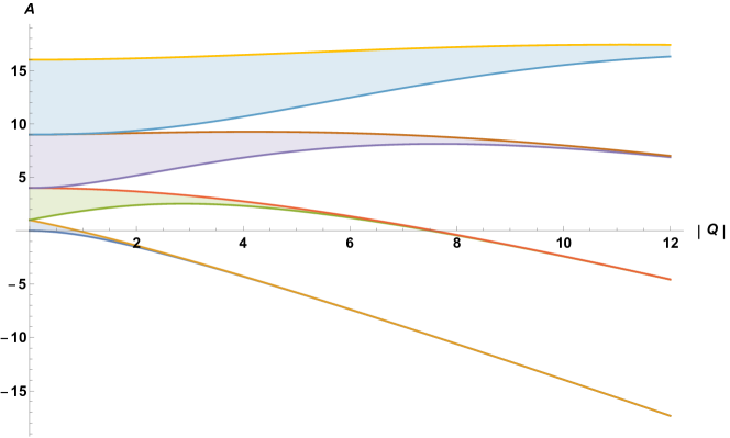
Figure 1: Stability chart of the Mathieu equation. In the colored regions (bands), the solutions are bounded. Landau levels emerge from the band spectrum as $|Q|\rightarrow\infty$.

The same conclusion can be drawn in a finite volume. In this case, the solutions in a band (the Bloch wave functions), do not obey, in general, periodic boundary conditions. The requirement of periodicity, $f(z+\pi)=f(z)$, picks out one level from the band. Such levels form the so-called characteristic curves $A_{n}(Q)$, which eventually approach the Landau levels as $Q\rightarrow\infty$.

III.6 Applicability of the perturbation theory in $B$

The applicability of the main formula Eq. (61) is limited, since its derivation relies on a perturbative expansion of the energy shift in the external field strength $B$. In Ref. Agadjanov:2016cjc , we have made a crude estimate for the upper bound on the magnitude of $B$ by considering a single period as a potential well. The condition that no bound states are formed in this potential well has led to the relation $eB<2\omega^{2}$. We are now in a position to provide a more stringent estimate, which is based on the properties of the solutions of the Mathieu equation. To this end, we consider another limiting case, when $B\rightarrow 0$ while the frequency $\omega$ is fixed. Since $q=O(B)$ and $p=O(B^{2})$, from Eq. (82) we again arrive at the Mathieu equation:

$$\left[\frac{d^{2}}{dz^{2}}+a-2q\cos(2z)\right]f(z)=0\,.$$ (88)

The structure of the finite-volume spectrum is shown in Fig. 2.

Figure 2: Finite-volume spectrum of the Mathieu equation.

The expansion of the ground state level $a_{0}$ in small $q$ reads AS

$$a_{0}=-\frac{q^{2}}{2}+O(q^{4})\,,$$ (89)

A similar formula can be written by using exact power series for $a_{0}$ in small $p$ and $q$, see Ref. Urwin . In particular, the first terms in these expansions coincide.

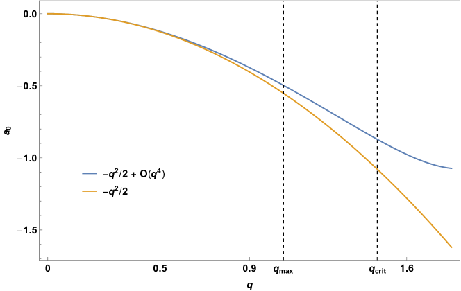
Figure 3: The ground state level $a_{0}(q)$ as a function of $q$. The critical value $q_{crit}\approx 1.47$ denotes the radius of convergence of the expansion in Eq. (89). At $q_{max}\approx 1.05$, the higher order corrections amount to a $10\%$ of the leading piece.

The perturbative expansion of $a_{0}$ in small $q$, Eq. (89), has a certain finite radius of convergence $q=q_{crit}$. This critical value provides an upper bound on the field strength $B$. One obtains for the proton and neutron, respectively:

$$eB<\frac{q_{crit}\omega^{2}}{2(1+\kappa_{p})}\,,\quad eB<\frac{q_{crit}\omega^{2}}{2|\kappa_{n}|}\,,$$ (90)

with $\kappa_{p}=1.79$ and $\kappa_{n}=-1.91$. In case of the neutron, the numerical value of the radius of convergence reads $q_{crit}\approx 1.47$ (see also Ref. Meixner ). For an estimate we use the same value for the proton. This is justified since in the limit $B\rightarrow 0$, Eq. (82) can be well approximated by the Mathieu equation. Accordingly, one obtains $eB<0.26\omega^{2}$ (proton) and $eB<0.38\omega^{2}$ (neutron).

The upper bound on the magnetic field strength in Eq. (90) can be improved by noting that our perturbative result, Eq. (61), might not be applicable at $q=q_{crit}$. To estimate higher order corrections, we can again resort to Eq. (89). In Fig. 3 we plot the function $a_{0}(q)$ as well as the first term in Eq. (89). As is seen, the higher order terms become large at $q=q_{crit}$ and hence can not be neglected anymore. Accordingly, it is plausible to choose a certain value $q=q_{max}$, for which they, e.g., amount to a $10\%$ of the leading piece. This gives $q_{max}\approx 1.05$ (see also Fig. 3). Using Eq. (90) we get an improved bound on the magnitude $B$: $eB<0.19\omega^{2}$ and $eB<0.27\omega^{2}$ for the proton and the neutron, respectively.

It interesting to note that Eq. (89) allows us to verify the main result, Eq. (61), in the approximation where the proton is treated as a point-like particle but with a non-zero anomalous magnetic moment. This is equivalent to setting $F_{1}=1$, $F_{2}=\kappa$ and $\beta_{M}=0$ in Eqs. (10,11). The subtraction function takes the value

$$S_{1}(-\omega^{2})=-\frac{1}{\omega^{2}}\left[(1+\kappa)^{2}-1\right]\,.$$ (91)

It is seen from Eq. (89) that there is no spin-dependent contribution to $a_{0}$. Using Eq. (83), we get directly the spin-averaged energy shift:

$$\delta E=-\frac{e^{2}B^{2}}{4m\omega^{2}}\left[(1+\kappa)^{2}-1\right]\,,$$ (92)

where we have used the relation $E^{2}-m^{2}\approx 2m\delta E$. This is precisely the expression which is obtained from the main formula in Eq. (61), when we substitute the subtraction function given in Eq. (91).

The above discussion is equally applicable for the neutron, for which $g=0$. In particular, the differential equation for $F(\mathbf{x})$, Eq. (78), simplifies:

$$[{\mathbf{p}}^{2}-\kappa\boldsymbol{\sigma}\cdot\mathbf{B}]F(\mathbf{x})=(E^{2}-m^{2})F(\mathbf{x})\,.$$ (93)

It can be brought into the form of the Mathieu equation:

$$\left[\frac{d^{2}}{dz^{2}}+a^{\prime}-2q^{\prime}\cos(2z)\right]f(z)=0\,,$$ (94)

where

$$a^{\prime}=\frac{4}{\omega^{2}}\left(E^{2}-m^{2}\right)\,\quad q^{\prime}=\alpha\frac{2\kappa eB}{\omega^{2}}\,.$$ (95)

As expected, no Landau levels emerge in the zero frequency limit $\omega\rightarrow 0$. Further, the main formula in Eq. (61) can be verified in a similar manner by setting $F_{1}=0$, $F_{2}=\kappa$ and $\beta_{M}=0$ in Eqs. (10,11). The spin-averaged energy shift reads

$$\delta E=-\frac{e^{2}B^{2}}{4m\omega^{2}}\kappa^{2}\,.$$ (96)

IV Propagator in an external field

The derivation based on the non-relativistic framework, which was given in the previous section, is not well suited for the study of the (exponentially suppressed) finite-volume effects. For example, the final result, displayed in Eq. (61), contains the infinite-volume Compton amplitude on the right-hand side, i.e., the finite-volume effects are neglected there. In the non-relativistic framework, these effects may emerge from different sources. First, the non-relativistic couplings contain the finite-volume corrections which, generally, go as $\exp(-M_{\pi}L)$ for large $L$ (we remind the reader that the lightest hadron mass gives the hard scale of the non-relativistic approach). Second, the Lagrangian contains operators which break rotational invariance but preserve octahedral symmetry. These operators are multiplied by the couplings that vanish exponentially for large values of $L$. Finally, in a finite volume, one may construct a new type of gauge-invariant operators (the Wilson line), which are absent in the infinite volume and whose contribution is also multiplied by exponentially suppressed couplings. Matching to the Chiral Perturbation Theory (ChPT) with the external field in a finite volume uniquely determines all these couplings. For a detailed discussion of these issues we refer the reader to Refs. Detmold:2006vu ; Hu:2007eb ; Hu:2007ts ; Tiburzi:2007ep ; Tiburzi:2008pa ; Tiburzi:2014zva .

From the above discussion it is clear that, in order to evaluate the finite-volume effects, it is better to work directly with ChPT in a finite volume, abandoning the non-relativistic framework, which has proven very convenient for discussing the zero-frequency limit. The exponentially suppressed finite-volume effects, which are not taken into account in ChPT, go as $\exp(-\Lambda_{H}L)$ instead of $\exp(-M_{\pi}L)$ (here, $\Lambda_{H}$ denotes a typical hadronic scale of order of one GeV), and thus can be neglected.

One important remark is in order. A procedure, which is used in Refs. Detmold:2006vu ; Hu:2007eb ; Hu:2007ts ; Tiburzi:2007ep ; Tiburzi:2008pa ; Tiburzi:2014zva for the extraction of the polarizabilities in a finite volume, boils down to the derivation of the finite-volume one-particle effective action and to the identification of the different terms in this action. In this way, one again encounters the problem with operators containing Wilson lines that makes e.g., the authors of Ref. Hu:2007ts to conclude that “At finite volume, there is no longer a discernible relation between polarizabilities and the Compton tensor.” In our framework we shall choose a different path, directly relating the amplitude for forward Compton scattering in a finite volume to the second-order energy shift of the nucleon in the external magnetic field. We are not asking ourselves, what the subtraction function is in a finite volume – this question anyway does not have an unique answer and, making an inconvenient choice, one can easily obscure the relation between the infinite- and finite-volume quantities. Rather, we can uniquely identify the quantity that is extracted from the nucleon energy shift in a finite volume and which reduces to the subtraction function in the limit $L\to\infty$ (as we shall see below, this is a certain component of the spin-averaged Compton tensor in a particular kinematics). This fully suffices to define a finite-volume counterpart of the subtraction function $S_{1}(q^{2})$ and to calculate finite-volume corrections in an unambiguous way.

In this section, using the framework of the effective field theory in a finite volume, we shall derive the expression for the nucleon energy shift in an external field (a finite-volume analog of Eq. (61)). Note also that we shall never specify the Lagrangian of this theory – it is only used to catalyze the proof and produce the diagrammatic expansion of all amplitudes in terms of hadronic propagators.

We start from the nucleon two-point function in the external field in Minkowski space and define:

$$\tilde{D}(x,y)=i\langle 0|T\Psi(x)\bar{\Psi}(y)|0\rangle_{A}\,,$$ (97)

where $\Psi(x)$ denotes the four-component spinor field, describing the nucleon. Note that the Dirac indices are not shown explicitly. Since the external field does not depend on time, we have $\tilde{D}(x,y)=\tilde{D}(x^{0}-y^{0};\mathbf{x},\mathbf{y})$. Further, it is convenient to define the Fourier transform in the fourth component

$$\tilde{D}(\mathbf{x},\mathbf{y};E)=\int_{-\infty}^{\infty}dz^{0}e^{iEz^{0}}\,\tilde{D}(z^{0};\mathbf{x},\mathbf{y})\,,$$ (98)

as well as in vector components,

$$D(\mathbf{p},\mathbf{k};E)=\int_{-L/2}^{L/2}d^{3}\mathbf{x}d^{3}\mathbf{y}\,e^{-i\mathbf{p}\mathbf{x}+i\mathbf{k}\mathbf{y}}\tilde{D}(\mathbf{x},\mathbf{y};E)\,.$$ (99)

One can invert this expression, giving

$$\tilde{D}(\mathbf{x},\mathbf{y};E)=\frac{1}{L^{3}}\sum_{\mathbf{p}}\frac{1}{L^{3}}\sum_{\mathbf{k}}\,e^{i\mathbf{p}\mathbf{x}-i\mathbf{k}\mathbf{y}}D(\mathbf{p},\mathbf{k};E)\,.$$ (100)

The free propagator takes the form:

$$D^{(0)}(\mathbf{p};\mathbf{k};E)=D^{(0)}(\mathbf{p};E)L^{3}\delta_{\mathbf{p}\mathbf{k}}\,,\quad\quad D^{(0)}(\mathbf{p};E)=\frac{m+\gamma_{0}E-\boldsymbol{\gamma}\mathbf{p}}{m^{2}-E^{2}+\mathbf{p}^{2}-i\epsilon}\,,$$ (101)

where $m$ is the physical nucleon mass.

Figure 4: Diagrammatic representation of the propagator in an external electromagnetic field. The third and fourth diagrams correspond to the one-particle reducible and one-particle irreducible contributions at $O(B^{2})$, respectively.

The diagrammatic representation of the propagator in the external electromagnetic field is schematically shown in Fig. 4. We have

$$D(\mathbf{p},\mathbf{k};E) = D^{(0)}(\mathbf{p};E)L^{3}\delta_{\mathbf{p}\mathbf{k}}+D^{(0)}(\mathbf{p};E)\Sigma(\mathbf{p},\mathbf{k};E)D^{(0)}(\mathbf{k};E)$$ (102)

$$+ \frac{1}{L^{3}}\sum_{\mathbf{l}}\,D^{(0)}(\mathbf{p};E)\Sigma(\mathbf{p},\mathbf{l};E)D^{(0)}(\mathbf{l};E)\Sigma(\mathbf{l},\mathbf{k};E)D^{(0)}(\mathbf{k};E)+\cdots\,,$$

where the self-energy part $\Sigma(\mathbf{p},\mathbf{k};E)$, which is a matrix in the space of Dirac indices, can be expanded in powers of the magnitude of the external field:

$$\Sigma(\mathbf{p},\mathbf{k};E)=\Sigma_{0}(\mathbf{p},\mathbf{k};E)+(eB)\Sigma_{1}(\mathbf{p},\mathbf{k};E)+(eB)^{2}\Sigma_{2}(\mathbf{p},\mathbf{k};E)+\cdots\,.$$ (103)

Here, $\Sigma_{0}(\mathbf{p},\mathbf{k};E)=L^{3}\delta_{{\bf p}{\bf k}}\Sigma_{0}(\mathbf{p};E)$ is the sum of all one-particle irreducible diagrams in the absence of the external field, and the functions $\Sigma_{1},\Sigma_{2}$ will be determined below. Note also that we use the MOM renormalization scheme, i.e., $\Sigma_{0}(\mathbf{p};\sqrt{m^{2}+{\bf p}^{2}})=0$. The sum in Eq. (102) can be written in a compact form:

$$D(\mathbf{p},\mathbf{k};E)=D^{(0)}(\mathbf{p};E)L^{3}\delta_{\mathbf{p}\mathbf{k}}+D^{(0)}(\mathbf{p};E)T(\mathbf{p},\mathbf{k};E)D^{(0)}(\mathbf{k};E)\,,$$ (104)

where the amplitude $T(\mathbf{p},\mathbf{k};E)$ satisfies the relation

$$T(\mathbf{p},\mathbf{k};E)=\Sigma(\mathbf{p},\mathbf{k};E)+\frac{1}{L^{3}}\sum_{\mathbf{l}}\,\Sigma(\mathbf{p},\mathbf{l};E)D^{(0)}(\mathbf{l};E)T(\mathbf{l},\mathbf{k};E)\,,$$ (105)

which is similar to the Lippmann-Schwinger equation.

In order to find the energy shift of the nucleon ground state, we have to determine the pole position in the propagator $D(\mathbf{0},\mathbf{0};E)$. For this purpose, we single out the term with ${\bf l}={\bf 0}$ in the sum (corresponding to the unperturbed ground state) and rewrite the amplitude $T(\mathbf{0},\mathbf{0};E)$ as follows:

$$T(\mathbf{0},\mathbf{0};E)=T^{\prime}(\mathbf{0},\mathbf{0};E)+\frac{1}{L^{3}}T^{\prime}(\mathbf{0},\mathbf{0};E)D^{(0)}(\mathbf{0};E)T(\mathbf{0},\mathbf{0};E)\,,$$ (106)

where the quantity $T^{\prime}(\mathbf{p},\mathbf{k};E)$ satisfies the equation

$$T^{\prime}(\mathbf{p},\mathbf{k};E)=\Sigma(\mathbf{p},\mathbf{k};E)+\frac{1}{L^{3}}\sum_{\mathbf{l}\neq 0}\,\Sigma(\mathbf{p},\mathbf{l};E)D^{(0)}(\mathbf{l};E)T^{\prime}(\mathbf{l},\mathbf{k};E)\,.$$ (107)

Note that now the sum runs over all $\mathbf{l}\neq 0$. We get

$$T(\mathbf{0},\mathbf{0};E)=\left(I-\frac{1}{L^{3}}T^{\prime}(\mathbf{0},\mathbf{0};E)D^{(0)}(\mathbf{0};E)\right)^{-1}T^{\prime}(\mathbf{0},\mathbf{0};E)\,.$$ (108)

Here, $I$ denotes the unit $4\times 4$ matrix. Inserting this expression into Eq. (104) for the propagator $D(\mathbf{0},\mathbf{0};E)$, one obtains

$$D(\mathbf{0},\mathbf{0};E)=D^{(0)}(\mathbf{0};E)L^{3}\left(I-\frac{1}{L^{3}}T^{\prime}(\mathbf{0},\mathbf{0};E)D^{(0)}(\mathbf{0};E)\right)^{-1}\,.$$ (109)

Obviously, $D(\mathbf{0},\mathbf{0};E)$ and $T(\mathbf{0},\mathbf{0};E)$ have the same pole structure.

In order to simplify the matrix equation (106), we can use the octahedral symmetry of the cubic lattice. For zero momenta, the symmetry requires that:

$$R_{\alpha\gamma}(g)T_{\gamma\delta}(\mathbf{0},\mathbf{0};E)R_{\delta\beta}(g^{-1})=T_{\alpha\beta}(\mathbf{0},\mathbf{0};E)\,,$$ (110)

where $g$ denotes an arbitrary element of the octahedral group and $R_{\alpha\beta}(g)$ is the matrix of the linear representation of the octahedral group which is obtained by restricting the $(1/2,0)+(0,1/2)$ representation of the Lorentz group to its octahedral subgroup (here the Greek letters denote Dirac indices). The requirement of invariance restricts $T_{\alpha\beta}(\mathbf{0},\mathbf{0};E)$ to the form:

$$T_{\alpha\beta}(\mathbf{0},\mathbf{0};E)=\delta_{\alpha\beta}T^{(1)}+(\gamma_{0})_{\alpha\beta}T^{(2)}\,,$$ (111)

where $T^{(1)}$ and $T^{(2)}$ are scalar functions. Accordingly, we see that

$$\bar{u}(\mathbf{0},s)T(\mathbf{0},\mathbf{0};E)u(\mathbf{0},s^{\prime}) = 2m\delta_{ss^{\prime}}(T^{(1)}+T^{(2)})\equiv 2m\delta_{ss^{\prime}}\tilde{T}\,,$$ (112)

$$\bar{v}(\mathbf{0},s)T(\mathbf{0},\mathbf{0};E)v(\mathbf{0},s^{\prime}) = -2m\delta_{ss^{\prime}}(T^{(1)}-T^{(2)})\,,$$ (113)

$$\bar{v}(\mathbf{0},s)T(\mathbf{0},\mathbf{0};E)u(\mathbf{0},s^{\prime}) = \bar{u}(\mathbf{0},s)T(\mathbf{0},\mathbf{0};E)v(\mathbf{0},s^{\prime})=0\,.$$ (114)

Similar relations can be established for the amplitude $T^{\prime}(\mathbf{0},\mathbf{0};E)$. For example, $\tilde{T}^{\prime}$ is defined through the equation

$$\bar{u}(\mathbf{0},s)T^{\prime}(\mathbf{0},\mathbf{0};E)u(\mathbf{0},s^{\prime})=2m\delta_{ss^{\prime}}\tilde{T}^{\prime}\,.$$ (115)

Further, it is convenient to write the free propagator $D_{\alpha\beta}^{(0)}(\mathbf{p};E)$ in the form

$$D_{\alpha\beta}^{(0)}(\mathbf{0};E)=\frac{1}{2m}\sum_{s}\frac{u_{\alpha}(\mathbf{0},s)\bar{u}_{\beta}(\mathbf{0},s)}{m-E}-\frac{1}{2m}\sum_{s}\frac{v_{\alpha}(\mathbf{0},s)\bar{v}_{\beta}(\mathbf{0},s)}{m+E}\,.$$ (116)

Multiplying the Eq. (106) by $\bar{u}(\mathbf{0},s)$ from the left and by $u(\mathbf{0},s)$ from the right, we get:

$$\tilde{T}=\tilde{T}^{\prime}+\frac{1}{L^{3}}\,\frac{1}{m-E}\tilde{T}^{\prime}\tilde{T}\,.$$ (117)

This equation is not a matrix equation anymore. The pole position is given by

$$m-E-\frac{1}{L^{3}}\tilde{T}^{\prime}=0\,,$$ (118)

As expected the free pole at $m-E=0$ has disappeared. This result is similar to the “master equation” in case of hadronic atoms Gasser:2007zt .

Next, let us proceed with the calculation of the amplitude $T^{\prime}(\mathbf{0},\mathbf{0};E)$. In perturbation theory, up-to-and-including $O(B^{2})$ this quantity reads

$$T^{\prime}(\mathbf{0},\mathbf{0};E) = \Sigma_{0}(\mathbf{0},\mathbf{0};E)+(eB)\Sigma_{1}(\mathbf{0},\mathbf{0};E)+(eB)^{2}\Sigma_{2}(\mathbf{0},\mathbf{0};E)$$ (119)

$$+ (eB)^{2}\frac{1}{L^{3}}\sum_{\mathbf{l}\neq 0}\,\Sigma_{1}(\mathbf{0},\mathbf{l};E)D^{(0)}(\mathbf{l};E)\Sigma_{1}(\mathbf{l},\mathbf{0};E)+\cdots$$

$$= T_{0}^{\prime}(\mathbf{0},\mathbf{0};E)+(eB)T_{1}^{\prime}(\mathbf{0},\mathbf{0};E)+(eB)^{2}T_{2}^{\prime}(\mathbf{0},\mathbf{0};E)+\cdots\,.$$

The quantity $\Sigma_{1}(\mathbf{p},\mathbf{k};E)$ can be expressed through the three-point vertex function. Indeed, consider the linear coupling to the external field which is described by the Lagrangian

$${\cal L}_{1}=-O_{1}(x)A^{1}(x)\,.$$ (120)

Here, we have used Eq. (13) which states that the vector potential has only one nonzero component $A^{1}$. The current operator $O_{1}$ contains both the nucleon and pion fields and obeys usual restrictions (hermiticity, certain transformation properties with respect to the Lorentz group, etc.) but, otherwise, its form can be arbitrary. Let us denote as $\tilde{D}_{1}(x,y)$ the respective contribution to the two-point function. At order $O(B)$, we then have:

$$\tilde{D}_{1}(x,y)=\int_{-L/2}^{L/2}d^{3}\mathbf{u}\int_{-\infty}^{\infty}du_{0}\,A^{1}(\mathbf{u})\langle 0|T\Psi(x)\bar{\Psi}(y)O_{1}(u)|0\rangle\,.$$ (121)

Further, using translational invariance, one can write

$$\langle 0|T\Psi(x)\bar{\Psi}(y)O_{1}(u)|0\rangle = \int_{-\infty}^{\infty}\frac{dp_{0}}{2\pi}\int_{-\infty}^{\infty}\frac{dk_{0}}{2\pi}\frac{1}{L^{3}}\sum_{\mathbf{p}}\frac{1}{L^{3}}\sum_{\mathbf{k}}\,e^{-ip(x-u)+ik(y-u)}$$ (122)

$$\times D^{(0)}(\mathbf{p},p_{0})\Gamma(p,k)D^{(0)}(\mathbf{k};k_{0})\,.$$

This is a definition of the vertex function $\Gamma(p;k)$. Substituting this expression into Eq. (121) and integrating over $u_{0}$ and $k_{0}$, we get

$$\tilde{D}_{1}(x,y) = \int_{-L/2}^{L/2}d^{3}\mathbf{u}\,A^{1}(\mathbf{u})\int_{-\infty}^{\infty}\frac{dp_{0}}{2\pi}\frac{1}{L^{3}}\sum_{\mathbf{p}}\frac{1}{L^{3}}\sum_{\mathbf{k}}\,e^{-ip_{0}(x_{0}-y_{0})}e^{i\mathbf{p}(\mathbf{x}-\mathbf{u})-i\mathbf{k}(\mathbf{y}-\mathbf{u})}$$ (123)

$$\times D^{(0)}(\mathbf{p};p_{0})\Gamma(\mathbf{p},\mathbf{k};E)D^{(0)}(\mathbf{k},p_{0})\,,$$

where $\Gamma(\mathbf{p},\mathbf{k};E)$ is obtained from $\Gamma(p,k)$ by substituting $p_{0}=k_{0}=E$ (we remind the reader that the field $A^{1}$ is static). Accordingly, the Fourier transform of $\tilde{D}_{1}(x,y)$ takes the simple form:

$$D_{1}(\mathbf{p},\mathbf{k};E)=\int_{-L/2}^{L/2}d^{3}\mathbf{u}\,A^{1}(\mathbf{u})e^{-i(\mathbf{p}-\mathbf{k})\mathbf{u}}D^{(0)}(\mathbf{p};E)\Gamma(\mathbf{p},\mathbf{k};E)D^{(0)}(\mathbf{k};E)\,.$$ (124)

Comparing this result with the expansion of the propagator in Eq. (102) at $O(B)$, it is seen that

$$(eB)\Sigma_{1}(\mathbf{p},\mathbf{k};E)=\Gamma(\mathbf{p},\mathbf{k};E)\int_{-L/2}^{L/2}d^{3}\mathbf{u}\,A^{1}(\mathbf{u})e^{-i(\mathbf{p}-\mathbf{k})\mathbf{u}}\doteq\Gamma(\mathbf{p},\mathbf{k};E)\tilde{A}^{1}({\bf k}-{\bf p})\,.$$ (125)

Next, we evaluate the quantity $\Sigma_{2}(\mathbf{p},\mathbf{k};E)$ which consists of all one-particle irreducible diagrams with amputated nucleon legs, with two external fields attached. Let $\Upsilon(p,k,l)$ denote the sum of all such diagrams in momentum space. Here, $p$ and $k$ denote the momenta of the outgoing and ingoing nucleon, respectively, and the momenta of two external “photons” are equal to $l+(k-p)/2$ and $l-(k-p)/2$, respectively. Further, denoting

$$\Upsilon({\bf p},{\bf k},{\bf l};E)=\Upsilon(p,k,l)\biggr{|}_{p_{0}=k_{0}=E,l_{0}=0}\,,$$ (126)

it is easy to check that $\Sigma_{2}$ is given by

$$(eB)^{2}\Sigma_{2}(\mathbf{p},\mathbf{k};E) = \int_{-L/2}^{L/2}d^{3}\mathbf{u}\int_{-L/2}^{L/2}d^{3}\mathbf{v}\,A^{1}(\mathbf{u})A^{1}(\mathbf{v})$$ (127)

$$\times \frac{1}{L^{3}}\sum_{\mathbf{l}}\,e^{i\mathbf{u}(\mathbf{l}+(\mathbf{k}-\mathbf{p})/2)-i\mathbf{v}(\mathbf{l}-(\mathbf{k}-\mathbf{p})/2)}\Upsilon(\mathbf{p},\mathbf{k},\mathbf{l};E)\,.$$

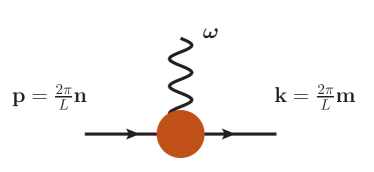
Figure 5: Three-momentum conservation in the $\gamma^{*}NN$ vertex gives the Kronecker delta $\delta_{\mathbf{p}-\mathbf{k},\pm\boldsymbol{\omega}}$.

We now have all ingredients for the evaluation of the energy shift. Here, following the discussion in the previous section, we consider the scenario a) for the external field, when the frequency $\omega$ is quantized and the three-momentum conservation holds. In this case, the term linear in $B$ gives:

$$(eB)T_{1}^{\prime}(\mathbf{p},\mathbf{k};E)=(eB)\Gamma(\mathbf{p},\mathbf{k};E)\frac{L^{3}}{2i\omega}[\delta_{-\mathbf{p}+\mathbf{k},-\boldsymbol{\omega}}-\delta_{-\mathbf{p}+\mathbf{k},\boldsymbol{\omega}}]\,.$$ (128)

Obviously, $\Sigma_{1}(\mathbf{0},\mathbf{0};E)=0$ for $\boldsymbol{\omega}\neq{\bf 0}$, see also Fig. 5.

The second-order term at threshold takes the form

$$(eB)^{2}T_{2}^{\prime}(\mathbf{0},\mathbf{0};m) = \frac{(eB)^{2}L^{3}}{4\omega^{2}}[\Upsilon(\mathbf{0},\mathbf{0},\boldsymbol{\omega};m)+\Upsilon(\mathbf{0},\mathbf{0},-\boldsymbol{\omega};m)]$$ (129)

$$+ \frac{(eB)^{2}L^{3}}{4\omega^{2}}\,\biggl{\{}\Gamma(\mathbf{0},\boldsymbol{\omega};m)D_{0}(\boldsymbol{\omega},m)\Gamma(\boldsymbol{\omega},\mathbf{0};m)$$

$$+ \Gamma(\mathbf{0},-\boldsymbol{\omega};m)D_{0}(-\boldsymbol{\omega},m)\Gamma(-\boldsymbol{\omega},\mathbf{0};m)\biggr{\}}\,.$$

On the other hand, it is straightforward to verify that the expression on the right-hand side of this equation is proportional to the “11” component of the forward Compton scattering tensor. Note also that, since $\boldsymbol{\omega}\neq{\bf 0}$, the sum over the intermediate nucleon states does not contain the term with ${\bf l}={\bf 0}$ and hence, there is no difference between $T_{2}$ and $T_{2}^{\prime}$ at threshold. Thus

$$\frac{Z(eB)^{2}}{2}\,\sum_{s}\bar{u}({\bf 0},s)T_{2}^{\prime}(\mathbf{0},\mathbf{0};m)u({\bf 0},s)=\frac{(eB)^{2}L^{3}}{2\omega^{2}}\,T^{11}(p,q)\,,$$ (130)

where $p^{\mu}=(m,{\bf 0})$, $q^{\mu}=(0,{\boldsymbol{\omega}})$ and the nucleon wave function renormalization constant (in the absence of the external field) is given by

$$Z^{-1} = 1+\frac{d}{dE}\,\tilde{\Sigma}_{0}(\mathbf{0};E)\biggr{|}_{E=m}\,,\quad\quad 2m\delta_{ss^{\prime}}\tilde{\Sigma}_{0}(\mathbf{0};E)=\bar{u}({\bf 0},s)\Sigma_{0}(\mathbf{0};E)u({\bf 0},s^{\prime})\,.$$ (131)

It is now straightforward to determine the spin-averaged energy shift at order $B^{2}$ from Eq. (118). Taking into account the fact that the linear term in $B$ vanishes, and expanding the quantity $\tilde{T}^{\prime}$ in Eq. (118) in Taylor series in $E-m$, it immediately follows that the spin-averaged energy shift is given by

$$\delta E = -\frac{Z(eB)^{2}}{2mL^{3}}\frac{1}{2}\sum_{s}\,\bar{u}(\mathbf{0},s)T_{2}^{\prime}(\mathbf{0},\mathbf{0};E)u(\mathbf{0},s)+O(B^{3})\,,$$ (132)

from which we finally obtain

$$\delta E=-\frac{1}{4m}\,\left(\frac{eB}{\omega}\right)^{2}T^{11}(p,q)+O(B^{3})\,.$$ (133)

This equation is the finite-volume version of Eq. (61) and contains the “11” component of the Compton tensor, evaluated in a finite volume. Up to the corrections, proportional to $\exp(-M_{\pi}L)$, this quantity is given by the subtraction function $S_{1}(q^{2})$ via $T^{11}(p,q)=-\omega^{2}S_{1}(q^{2})$, see Eqs. (6) and (II.1). Hence, the equation (133) provides a framework for the systematic calculation of such corrections.

V Discussion of the parameter range in numerical calculations

In Ref. Agadjanov:2016cjc we presented a brief discussion of the lattice parameters, which could be used in the numerical extraction of the subtraction function $S_{1}(q^{2})$. With the use of the new, more stringent constraints on the value of the magnetic field we are now able to refine this analysis. For a moment, we neglect the finite-volume corrections altogether. As in Ref. Agadjanov:2016cjc , the elastic and inelastic parts of the amplitude are parameterized as:

$$S_{1}^{el}(q^{2}) = -\frac{4m^{2}}{q^{2}(4m^{2}-q^{2})}\,\biggl{\{}G_{E}^{2}(q^{2})-G_{M}^{2}(q^{2})\biggr{\}}\,,$$

$$S_{1}^{inel}(q^{2}) = S_{1}^{inel}(0)G_{d}(q^{2})\,,\quad\quad S_{1}^{inel}(0)=-\frac{\kappa^{2}}{4m^{2}}-\frac{m}{\alpha}\,\beta_{M}\,,$$ (134)

where $\kappa$ and $\beta_{M}$ denote the anomalous magnetic moment and the magnetic polarizability of the nucleon (we use the same numerical values in the estimates as given in Ref. Agadjanov:2016cjc ). Further, $G_{d}(q^{2})=(1-q^{2}/0.71\mbox{\,GeV}^{2})^{-2}$ is the dipole form factor. It should be noted that the asymptotic behavior at large values of $q^{2}$ is consistent with the result of the operator product expansion in QCD.

The electric and magnetic form factors of the proton and the neutron are given by:

$$G_{E}^{p}(q^{2}) = G_{d}(q^{2})\,,\quad\quad G_{M}^{p}(q^{2})=(1+\kappa^{p})G_{d}(q^{2})\,,$$

$$G_{E}^{n}(q^{2}) = \frac{-q^{2}}{4m^{2}}\,\kappa^{n}G_{d}(q^{2})\,,\quad\quad G_{M}^{n}(q^{2})=\kappa^{n}G_{d}(q^{2})\,,$$ (135)

with the same dipole form factor as above.

One of the estimates, which goes through exactly in the same way as in Ref. Agadjanov:2016cjc , is related to our ability to separate the physically interesting inelastic part from total amplitude. As seen, the elastic part is singular at threshold and falls off very fast at higher $\omega^{2}$. Thus, the separation will be difficult for very small values of $\omega^{2}$. One may require, for instance, that at the minimum value of $\omega^{2}$, the inelastic contribution amounts up to a $10\%$ of the elastic contribution. In this manner, we get $\omega_{min}^{2}=0.086~{}\mbox{GeV}^{2}$ for the proton and $\omega_{min}^{2}=0.045~{}\mbox{GeV}^{2}$ for the neutron (a slight difference to the numbers given in Ref. Agadjanov:2016cjc is caused by the fact that here we take into account the exact momentum dependence of all amplitudes). If one requires instead that elastic and inelastic parts are equal, one gets $\omega_{min}^{2}=0.40~{}\mbox{GeV}^{2}$ for the proton and $\omega_{min}^{2}=0.26~{}\mbox{GeV}^{2}$ for the neutron. In any case, the lower cutoff on the available frequencies is rather comfortable and does not put significant restrictions on the parameters of the lattices which can be used in the calculations.

The conditions, which involve the magnitude of the magnetic field, are more restrictive. On one side, the magnetic field should be strong enough, in order to measure the effect at all. On the other hand, it must be weak enough, so that the perturbation theory still applies. In section III.6 we have made a more stringent estimate

$$eB<0.19\,\omega^{2}\quad\mbox{(proton),}\quad\quad eB<0.27\,\omega^{2}\quad\mbox{(neutron),}$$ (136)

which is based on the properties of the solutions of Mathieu’s equation. Denoting the inelastic shift by $\delta E^{inel}$, according to Ref. Agadjanov:2016cjc , we get

$$eB = \biggl{(}\frac{4m\delta E^{inel}}{S_{1}^{inel}(0)}\biggr{)}^{1/2}G_{d}^{-1/2}(-\omega^{2})<0.19\omega^{2}\quad\mbox{(for proton),}$$

$$eB = \biggl{(}\frac{4m\delta E^{inel}}{S_{1}^{inel}(0)}\biggr{)}^{1/2}G_{d}^{-1/2}(-\omega^{2})<0.27\omega^{2}\quad\mbox{(for neutron).}$$ (137)

It is now clear that the window for the available values of $eB$ exists if and only if $\delta E^{inel}$ can be taken sufficiently small or, in other words, if the uncertainty in the determination of $\delta E^{inel}$ does not exceed certain value. Generously allowing this uncertainty to be $\delta E^{inel}=0.05m$, as done in Ref. Agadjanov:2016cjc , is no more an option - the inequalities in Eq. (V) can not be satisfied. A better accuracy in the determination of the energy shift $\delta E^{inel}=0.01m$ would lead to the lower cutoff on the available frequencies $\omega_{min}^{2}=0.90~{}\mbox{GeV}^{2}$ for the proton and $\omega_{min}^{2}=0.41~{}\mbox{GeV}^{2}$ for the neutron. If one wants to increase the range of available frequencies and reach lower values of $\omega^{2}$, one has to improve on the accuracy further. The range of the magnitudes for the magnetic field can be determined from the above equations, if the accuracy is given.

VI Conclusions and Outlook

• We have presented three alternative derivations (the third one is contained in the appendix) of the formula for the energy shift of the nucleon, placed in a periodic external field. Namely, the non-relativistic effective Lagrangian was used for this purpose, as well as the relativistic framework. All these alternative settings are advantageous for discussing different issues arising in the treatment of the problem. The aim of the whole exercise is to extract the forward Compton scattering amplitude in a certain kinematics, the so-called subtraction function $S_{1}(q^{2})$, from lattice simulations. In its turn, measuring this function would enable one to gain important information about the properties of QCD at low energy.

• The result or Ref. Agadjanov:2016cjc has been refined and extended in various aspects. For example, in this paper we discuss in detail the zero-frequency limit (constant magnetic field) of the expression for the energy shift. This limiting case is studied in the literature in detail. Here, it is shown that, to have a smooth transition to this limit, the external field on the lattice should be implemented in a specific way, corresponding to the scenario b). There exists no zero-frequency limit for scenario a).

• Another important issue is the limit of validity of the perturbative treatment of the external magnetic field (the convergence radius of the perturbative expansion in $B$). In Ref. Agadjanov:2016cjc , using heuristic arguments, we gave a rough estimate of the maximal field strength, for which the perturbative approach is still applicable. In the present paper we improved the argument and give a new, much more stringent estimate, which is based on the properties of the solutions of Mathieu’s equation. It should be pointed out that the non-relativistic EFT approach provides the most convenient framework for the discussion of the above two problems.

• We have generalized the result of Ref. Agadjanov:2016cjc and derived an equation which relates the energy shift to the “11” component of the Compton tensor in a finite volume. Using this formula, one may estimate the exponentially suppressed finite-volume corrections to the extracted value of the subtraction function. This can be done, e.g., by performing calculations at one loop in ChPT in a finite volume. The calculations are under way and the results will be reported elsewhere Lozano . The preliminary results show that the finite-volume corrections at one loop in ChPT are sizable, but can be kept under control at reasonably large lattice volumes $M_{\pi}L>4$. Moreover, one might use a similar setting to estimate the effects of partial (electro)quenching in lattice simulations.

*

Appendix A Alternative derivation of Eq. (133).

For the sake of completeness, we present yet another derivation of the main formula for the energy shift given in Eq. (133), which is based on the study of the two-point function of the nucleon field in the external field at large time separation and, hence, has a closer resemblance to the methods used on the lattice. It is assumed that the external field is implemented according to scenario a), i.e., the frequency is quantized. In this derivation, we directly expand the nucleon two-point function in the external field

$$C=C^{(0)}+C^{(1)}+C^{(2)}+O(A^{3}),$$ (138)

where

$$C = \frac{1}{L^{3}}\int_{-L/2}^{L/2}d^{3}{\bf x}d^{3}{\bf y}\,\langle 0|T\Psi(x)\bar{\Psi}(y)|0\rangle_{A}\,,$$ (139)

$$C^{(0)} = \frac{1}{L^{3}}\int_{-L/2}^{L/2}d^{3}{\bf x}d^{3}{\bf y}\,\langle 0|T\Psi(x)\bar{\Psi}(y)|0\rangle\,,$$ (140)

$$C^{(1)} = \frac{i}{L^{3}}\int_{-L/2}^{L/2}d^{3}{\bf x}d^{3}{\bf y}d^{4}z\,A_{\mu}(\mathbf{z})\langle 0|T\Psi(x)\bar{\Psi}(y)j^{\mu}(z)|0\rangle\,,$$ (141)

$$C^{(2)} = \frac{i^{2}}{2L^{3}}\int_{-L/2}^{L/2}d^{3}{\bf x}d^{3}{\bf y}d^{4}zd^{4}v\,A_{\mu}(\mathbf{z})A_{\nu}(\mathbf{v})\langle 0|T\Psi(x)\bar{\Psi}(y)j^{\mu}(z)j^{\nu}(v)|0\rangle\,.$$ (142)

Here, the integration over $d^{3}{\bf x}d^{3}{\bf y}$ projects onto the states with zero initial and final three-momenta.

Note that, strictly speaking, for a rigorous derivation one should perform the Wick rotation into the Euclidean space and pick up the leading terms in the two-point function at large (Euclidean) times. For simplicity, however, we stay in the Minkowski space and identify the leading exponentials there – in our case, the identification is easy and no ambiguities arise.

The completeness condition, which we shall be using, takes the form

$$\frac{1}{L^{3}}\sum_{\mathbf{k}s}\,\frac{|\mathbf{k},s\rangle\langle\mathbf{k},s|}{2\omega(\mathbf{k})}+\cdots=1\,,$$ (143)

where ellipses stand for the excited states contributions; they will be neglected altogether by taking the limit $x_{0}-y_{0}\to\infty$ (the time extent of the lattice is assumed to be infinite).

Let us start with the matrix element $C^{(0)}$ that describes the propagation of the nucleon in the absence of the external field. Using the translation invariance, it takes the form

$$C^{(0)} = \frac{1}{L^{6}}\sum_{\mathbf{k}s}\frac{1}{2w(\mathbf{k})}\int_{-L/2}^{L/2}d^{3}\mathbf{x}d^{3}\mathbf{y}\,\theta(x_{0}-y_{0})e^{i\mathbf{k}(\mathbf{x}-\mathbf{y})}e^{-iw(\mathbf{k})(x_{0}-y_{0})}\langle 0|\Psi(0)|\mathbf{k},s\rangle\langle\mathbf{k},s|\bar{\Psi}(0)|0\rangle$$ (144)

$$+ \cdots\,.$$

Note that the second term in the $T$-product, containing $\theta(y_{0}-x_{0})$, picks up the antiparticle pole for large $x_{0}-y_{0}$ instead of the particle pole, and thus can be neglected.

Integrating over all variables, one gets

$$C^{(0)}=\sum_{s}\frac{e^{-im(x_{0}-y_{0})}}{2m}\,\langle 0|\Psi(0)|\mathbf{0},s\rangle\langle\mathbf{0},s|\bar{\Psi}(0)|0\rangle+\cdots\,.$$ (145)

Taking into account that

$$\langle 0|\Psi(0)|{\bf 0},s\rangle=Z^{1/2}u({\bf 0},s)\,,$$ (146)

where $Z$ denotes the wave function renormalization constant, we may write

$$\bar{u}({\bf 0},s)C^{(0)}u({\bf 0},s)=2mZe^{-im(x_{0}-y_{0})}+\cdots\,.$$ (147)

The two-point function in the presence of the external magnetic field can be written in a similar manner:

$$\bar{u}({\bf 0},s)Cu({\bf 0},s)=2E_{s}(B)Z_{s}(B)e^{-iE_{s}(B)(x_{0}-y_{0})}+\cdots$$ (148)

Here, $E_{s}(B)$ is the energy of the nucleon ground state. Note that, in general, $E_{s}(B)$ and $Z_{s}(B)$ depend on the orientation of the spin $s$. The functions $E_{s}(B)$ and $Z_{s}(B)$ can be expanded in $B$:

$$E_{s}(B) = m+\xi_{s}(\omega)(eB)+\eta_{s}(\omega)(eB)^{2}+O(B^{3})\,,$$

$$Z_{s}(B) = Z+\alpha_{s}(\omega)(eB)+\beta_{s}(\omega)(eB)^{2}+O(B^{3})\,.$$ (149)

The unknown quantities $\xi_{s}(\omega),\eta_{s}(\omega),\alpha_{s}(\omega),$ and $\beta_{s}(\omega)$ depend on the frequency $\omega$.

The correlator $C^{(1)}$ is evaluated in a similar manner to $C^{(0)}$. The only contribution remaining at $x_{0}-y_{0}\to\infty$ is given by

$$C^{(1)} = \frac{i}{L^{9}}\sum_{\mathbf{k}s,\mathbf{l}s^{\prime}}\frac{1}{4w(\mathbf{k})w(\mathbf{l})}\int_{-L/2}^{L/2}d^{3}\mathbf{x}d^{3}\mathbf{y}d^{3}\mathbf{z}dz_{0}\,A^{1}(\mathbf{z})\theta(x_{0}-z_{0})\theta(z_{0}-y_{0})$$

$$\times e^{i\mathbf{k}(\mathbf{x}-\mathbf{z})}e^{-iw(\mathbf{k})(x_{0}-z_{0})}e^{i\mathbf{l}(\mathbf{z}-\mathbf{y})}e^{-iw(\mathbf{l})(z_{0}-y_{0})}\langle 0|\Psi(0)|\mathbf{k},s\rangle\langle\mathbf{k},s|j^{1}(0)|\mathbf{l},s^{\prime}\rangle\langle\mathbf{l},s^{\prime}|\bar{\Psi}(0)|0\rangle+\cdots\,.$$

After the summation over the three-momentum the above expression simplifies and we get:

$$\bar{u}({\bf 0},s)C^{(1)}u({\bf 0},s)=i\frac{Ze^{-im(x_{0}-y_{0})}}{L^{3}}(x_{0}-y_{0})\langle\mathbf{0},s|j^{1}(0)|\mathbf{0},s\rangle\int_{-L/2}^{L/2}d^{3}\mathbf{z}\,A^{1}(\mathbf{z})+\cdots\,,$$ (151)

The integral over the periodic electromagnetic potential vanishes, and so

$$C^{(1)}=0.$$ (152)

The calculation of the second-order matrix element $C^{(2)}$ proceeds similarly. First inserting the completeness relation and using the translational invariance, one gets

$$\bar{u}({\bf 0},s)C^{(2)}u({\bf 0},s) = i^{2}\frac{Ze^{-im(x_{0}-y_{0})}}{2L^{3}}\int_{-L/2}^{L/2}d^{3}\mathbf{z}d^{3}\mathbf{v}d\lambda_{0}dv_{0}\,A^{1}(\mathbf{z})A^{1}(\mathbf{v})\theta(x_{0}-\lambda_{0}-v_{0})\theta(v_{0}-y_{0})$$ (153)

$$\times \langle\mathbf{0},s|Tj^{1}(\lambda)j^{1}(0)|\mathbf{0},s\rangle+\cdots\,,$$

where $\lambda_{0}=z_{0}-v_{0}$ is a new integration variable, and we have introduced the new four-vector $\lambda=(\lambda_{0},\mathbf{z}-\mathbf{v})$. It is then straightforward to verify the identity

$$\langle\mathbf{0},s|Tj^{1}(\lambda)j^{1}(0)|\mathbf{0},s\rangle=-\frac{2i}{L^{3}}\sum_{\mathbf{q}}\int_{-\infty}^{\infty}\,\frac{dq_{0}}{2\pi}e^{-iq\lambda}T^{11}({\bf 0},s;{\bf 0},s;q)\,,\quad\lambda=z-v\,.$$ (154)

Here, $T^{11}$ is the “11” component of the Compton tensor (before spin averaging) in a finite volume. We further get

$$\bar{u}({\bf 0},s)C^{(2)}u({\bf 0},s) = i\frac{Ze^{-im(x_{0}-y_{0})}}{L^{6}}\,\sum_{\mathbf{q}}\int_{-\infty}^{\infty}\,\frac{dq_{0}}{2\pi}\int_{-L/2}^{L/2}d^{3}\mathbf{z}d^{3}\mathbf{v}d\lambda_{0}dv_{0}$$ (155)

$$\times A^{1}(\mathbf{z})A^{1}(\mathbf{v})\theta(x_{0}-\lambda_{0}-v_{0})\theta(v_{0}-y_{0})e^{-iq\lambda}T^{11}({\bf 0},s;{\bf 0},s;q)+\cdots\,.\qquad$$

Next, the integration over $v_{0}$ gives

$$\int_{-\infty}^{\infty}dv_{0}\,\theta(x_{0}-\lambda_{0}-v_{0})\theta(v_{0}-y_{0})=(x_{0}-y_{0}-\lambda_{0})\theta(x_{0}-y_{0}-\lambda_{0})\,.$$ (156)

Accordingly,

$$\bar{u}({\bf 0},s)C^{(2)}u({\bf 0},s)=i\frac{Ze^{-im(x_{0}-y_{0})}}{L^{6}}\,\sum_{\mathbf{q}}\,\tilde{A}^{1}(\mathbf{q})\tilde{A}^{1}(-\mathbf{q})I({\bf 0},s;{\bf 0},s;\mathbf{q})+\cdots\,,$$ (157)

where $\tilde{A}^{1}(\mathbf{q})$ is defined in Eq. (43). The quantity $I({\bf 0},s;{\bf 0},s;\mathbf{q})$ reads

$$I({\bf 0},s;{\bf 0},s;\mathbf{q})=\int_{-\infty}^{\infty}\,\frac{dq_{0}}{2\pi}\int_{-\infty}^{x_{0}-y_{0}}\,d\lambda_{0}\,(x_{0}-y_{0}-\lambda_{0})e^{-iq_{0}\lambda_{0}}T^{11}({\bf 0},s;{\bf 0},s;q)\,.$$ (158)

The shift of the variable $\lambda_{0}\rightarrow x_{0}-y_{0}-\lambda_{0}$ and partial integration over $q_{0}$ gives

$$I({\bf 0},s;{\bf 0},s;\mathbf{q})=i\int_{-\infty}^{\infty}\,\frac{dq_{0}}{2\pi}\int_{0}^{\infty}\,d\lambda_{0}\,e^{iq_{0}\lambda_{0}}\frac{\partial}{\partial q_{0}}\left[e^{-iq_{0}(x_{0}-y_{0})}T^{11}({\bf 0},s;{\bf 0},s;q)\right]\,.$$ (159)

Integrating over $\lambda_{0}$, one obtains

$$I({\bf 0},s;{\bf 0},s;\mathbf{q})=-\int_{-\infty}^{\infty}\,\frac{dq_{0}}{2\pi}\frac{e^{-iq_{0}(x_{0}-y_{0})}}{q_{0}+i\epsilon}\left[-i(x_{0}-y_{0})T^{11}({\bf 0},s;{\bf 0},s;q)+\frac{\partial}{\partial q_{0}}T^{11}({\bf 0},s;{\bf 0},s;q)\right]\,,$$ (160)

where the $i\epsilon$ prescription ensures the convergence of the integral. Further, contour integration leads to the following expression:

$$I({\bf 0},s;{\bf 0},s;\mathbf{q})=(x_{0}-y_{0})T^{11}({\bf 0},s;{\bf 0},s;\bar{q})+i\frac{\partial}{\partial q_{0}}T^{11}({\bf 0},s;{\bf 0},s;q)\Big{|}_{q=\bar{q}}\,,\quad\bar{q}=(0,\mathbf{q})\,.$$ (161)

Finally, inserting this result into Eq. (157) and summing over $\mathbf{q}$, the correlator $C^{(2)}$ takes the value

$$\bar{u}({\bf 0},s)C^{(2)}u({\bf 0},s) = i\frac{Ze^{-im(x_{0}-y_{0})}}{2}\left(\frac{eB}{\omega}\right)^{2}\bigg{[}(x_{0}-y_{0})T^{11}({\bf 0},s;{\bf 0},s;\hat{q})$$ (162)

$$+ \frac{i}{2}\frac{\partial}{\partial q_{0}}T^{11}({\bf 0},s;{\bf 0},s;q)\Big{|}_{q=\hat{q}}+\frac{i}{2}\frac{\partial}{\partial q_{0}}T^{11}({\bf 0},s;{\bf 0},s;q)\Big{|}_{q=-\hat{q}}\bigg{]}+\cdots\,,$$

where the symmetry property of the Compton tensor, $T^{11}({\bf 0},s;{\bf 0},s;\hat{q})=T^{11}({\bf 0},s;{\bf 0},s;-\hat{q})$, $\,\hat{q}=(0,\boldsymbol{\omega})$, was used.

Next, combining Eqs. (A) and (148), one gets the Taylor expansion of the two-point function in the magnetic field strength:

$$\bar{u}({\bf 0},s)Cu({\bf 0},s) = 2mZe^{-im(x_{0}-y_{0})}\biggl{\{}1+\frac{\alpha_{s}(\omega)(eB)+\beta_{s}(\omega)(eB)^{2}}{Z}+\frac{\xi_{s}(\omega)(eB)+\eta_{s}(\omega)(eB)^{2}}{m}$$

$$- i(x_{0}-y_{0})\left.\left[\frac{\xi_{s}(\omega)(eB)+\eta_{s}(\omega)(eB)^{2}}{m}\right]+\frac{\xi_{s}(\omega)\alpha_{s}(\omega)(eB)^{2}}{mZ}\right.$$

$$- i(x_{0}-y_{0})\frac{\xi_{s}(\omega)(eB)}{m}\,\left[\frac{\xi_{s}(\omega)(eB)}{m}+\frac{\alpha_{s}(\omega)(eB)}{Z}\right]+O(B^{3},(x_{0}-y_{0})^{2})\biggr{\}}\,.$$

The unknown coefficients $\xi_{s}(\omega)$ and $\eta_{s}(\omega)$ are determined from a comparison of the right-hand side in the above expansion with the known expression of $C$ up to and including $O(B^{2})$. This comparison gives the familiar result:

$$\xi_{s}(\omega)=0,\qquad\eta_{s}(\omega)=-\frac{1}{4m\omega^{2}}T^{11}({\bf 0},s;{\bf 0},s;\hat{q})\,.$$ (164)

The quantities $\alpha_{s}(\omega)$ and $\beta_{s}(\omega)$ can be found in a similar fashion. In particular, $\alpha_{s}(\omega)=0$, while $\beta_{s}(\omega)$ is given as a certain linear combination of the tensor component $T^{11}({\bf 0},s;{\bf 0},s;\hat{q})$ and its derivative. As it is seen, the first-order correction to the energy shift vanishes, while the spin-averaged second-order term reproduces Eq. (133).

References

- (1) A. Agadjanov, U.-G. Meißner and A. Rusetsky, Phys. Rev. D 95 (2017) 031502 [arXiv:1610.05545 [hep-lat]].
- (2) M. J. Savage et al., Phys. Rev. Lett. 119 (2017) 062002 [arXiv:1610.04545 [hep-lat]].
- (3) E. Chang et al. [NPLQCD Collaboration], Phys. Rev. D 92 (2015) 114502 [arXiv:1506.05518 [hep-lat]].
- (4) S. R. Beane et al., Phys. Rev. Lett. 113 (2014) 252001 [arXiv:1409.3556 [hep-lat]].
- (5) S. R. Beane et al. [NPLQCD Collaboration], Phys. Rev. Lett. 115 (2015) 132001 [arXiv:1505.02422 [hep-lat]].
- (6) A. J. Chambers et al., Phys. Rev. D 92 (2015) 114517 [arXiv:1508.06856 [hep-lat]].
- (7) A. J. Chambers et al. [CSSM and QCDSF/UKQCD Collaborations], Phys. Rev. D 90 (2014) 014510 [arXiv:1405.3019 [hep-lat]].
- (8) G. Bali and G. Endrödi, Phys. Rev. D 92 (2015) 054506 [arXiv:1506.08638 [hep-lat]].
- (9) A. J. Chambers et al. [QCDSF and UKQCD and CSSM Collaborations], Phys. Rev. D 96 (2017) 114509 [arXiv:1702.01513 [hep-lat]].
- (10) A. J. Chambers et al., Phys. Rev. Lett. 118 (2017) 242001 [arXiv:1703.01153 [hep-lat]].
- (11) Z. Davoudi and W. Detmold, Phys. Rev. D 92 (2015) 074506 [arXiv:1507.01908 [hep-lat]].
- (12) F. Hagelstein, R. Miskimen and V. Pascalutsa, Prog. Part. Nucl. Phys. 88 (2016) 29 [arXiv:1512.03765 [nucl-th]].
- (13) W. N. Cottingham, Annals Phys. 25 (1963) 424.
- (14) C. E. Carlson and M. Vanderhaeghen, Phys. Rev. A 84 (2011) 020102 [arXiv:1101.5965 [hep-ph]].
- (15) J. Gasser, M. Hoferichter, H. Leutwyler and A. Rusetsky, Eur. Phys. J. C 75 (2015) 375 [arXiv:1506.06747 [hep-ph]].
- (16) A. Walker-Loud, C. E. Carlson and G. A. Miller, Phys. Rev. Lett. 108 (2012) 232301 [arXiv:1203.0254 [nucl-th]].
- (17) F. B. Erben, P. E. Shanahan, A. W. Thomas and R. D. Young, Phys. Rev. C 90 (2014) 065205 [arXiv:1408.6628 [nucl-th]].
- (18) K. K. Cushman, A. W. Thomas and R. D. Young, arXiv:1804.05031 [nucl-th].
- (19) V. Bernard, T. R. Hemmert and U.-G. Meißner, Phys. Rev. D 67 (2003) 076008 [hep-ph/0212033].
- (20) C. Peset and A. Pineda, Nucl. Phys. B 887 (2014) 69 [arXiv:1406.4524 [hep-ph]].
- (21) V. Bernard, E. Epelbaum, H. Krebs and U.-G. Meißner, Phys. Rev. D 87 (2013) 054032 [arXiv:1209.2523 [hep-ph]].
- (22) J. Gasser and H. Leutwyler, Nucl. Phys. B 94 (1975) 269.
- (23) S. J. Brodsky, F. J. Llanes-Estrada and A. P. Szczepaniak, Phys. Rev. D 79 (2009) 033012 [arXiv:0812.0395 [hep-ph]].
- (24) M. Gorchtein, F. J. Llanes-Estrada and A. P. Szczepaniak, Phys. Rev. A 87 (2013) 052501 [arXiv:1302.2807 [nucl-th]].
- (25) R. Tarrach, Nuovo Cim. A 28 (1975) 409.
- (26) J. Bernabeu and R. Tarrach, Ann. Phys. 102 (1976) 323.
- (27) R. J. Hill and G. Paz, Phys. Rev. D 95 (2017) 094017 [arXiv:1611.09917 [hep-ph]].
- (28) R. J. Hill, G. Lee, G. Paz and M. P. Solon, Phys. Rev. D 87 (2013) 053017 [arXiv:1212.4508 [hep-ph]].
- (29) G. Colangelo, J. Gasser, B. Kubis and A. Rusetsky, Phys. Lett. B 638 (2006) 187 [hep-ph/0604084].
- (30) J. Gasser, B. Kubis and A. Rusetsky, Nucl. Phys. B 850 (2011) 96 [arXiv:1103.4273 [hep-ph]].
- (31) L. Landau and E. Lifshitz, Quantum Mechanics, 3rd ed., Course of Theoretical Physics (Pergamon Press, 1977).
- (32) C. Itzykson and J. B. Zuber, Quantum Field Theory (McGraw Hill, New York, 1980).
- (33) M. Abramowitz and I. A. Stegun, Handbook of mathematical functions: with formulas, graphs, and mathematical tables (Dover Publications, 1972).
- (34) K. Urwin, J. Inst. Maths. Applics. 3, 169 (1967).
- (35) J. Meixner, F. W. Schäfke and G. Wolf, Mathieu Functions and Spheroidal Functions and their Mathematical Foundations (Springer-Verlag, Berlin-New York, 1980).
- (36) W. Detmold, B. C. Tiburzi and A. Walker-Loud, Phys. Rev. D 73 (2006) 114505 [hep-lat/0603026].
- (37) J. Hu, F. J. Jiang and B. C. Tiburzi, Phys. Lett. B 653 (2007) 350 [arXiv:0706.3408 [hep-lat]].
- (38) J. Hu, F. J. Jiang and B. C. Tiburzi, Phys. Rev. D 77 (2008) 014502 [arXiv:0709.1955 [hep-lat]].
- (39) B. C. Tiburzi, Phys. Rev. D 77 (2008) 014510 [arXiv:0710.3577 [hep-lat]].
- (40) B. C. Tiburzi, Phys. Lett. B 674 (2009) 336 [arXiv:0809.1886 [hep-lat]].
- (41) B. C. Tiburzi, Phys. Rev. D 89 (2014) 074019 [arXiv:1403.0878 [hep-lat]].
- (42) J. Gasser, V. E. Lyubovitskij and A. Rusetsky, Phys. Rept. 456 (2008) 167 [arXiv:0711.3522 [hep-ph]].
- (43) J. Lozano et al., in progress.