The variance of the average depth of a pure birth process converges to 7

Abstract

If trees are constructed from a pure birth process and one defines the depth of a leaf to be the number of edges to its root, it is known that the variance in the depth of a randomly selected leaf of a randomly selected tree grows linearly in time. In this letter, we instead consider the variance of the average depth of leaves within each individual tree, establishing that, in contrast, it converges to a constant, $7$. This result indicates that while the variance in leaf depths amongst the ensemble of pure birth processes undergoes large fluctuations, the average depth across individual trees is much more consistent.

1 Introduction

Continuous time branching processes form fundamental building blocks of many stochastic models (e.g. [8]) and much is known about many statistics associated with them. A pure birth process [14] is the simplest continuous time branching process. It describes the growth of a directed tree that starts at time $0$ with a root, which is the first leaf. Each leaf extends the tree by creating two new leaves after an exponentially distributed time with mean $1/\lambda$, independently of everything else. Pure birth processes appear as a fundamental model of study in a large number of applications from data structures in computer science to likelihood methods in phylogenetics to the study of random walkers on random graphs, and are well studied.

Of interest to us here is a measure of tree depth, the distance from root to leaves. If one conditions on the number of nodes, much is known. For example, Pittel [12] linked prior results regarding binary search trees [15, 5, 3] to continuous time Markovian branching processes, establishing scaling properties of the depth of the both the shortest and longest leaf. Further extensions of those results have since been found  [13, 1]. Without conditioning on the number of nodes in the tree, relatively little appears in the literature. For a pure birth process, it is known that the mean depth of a randomly chosen leaf in a randomly selected tree grows as $2\lambda t$ with variance $2\lambda t$ [16]. However, for many applications, particularly in the life sciences e.g [11, 9], one is interested in the properties of individual growing trees. Denoting the number of leaves in a random tree at time $t$ by $Z(t)$ and the sum of their depths by $G(t)$, with $Z(0)=1$ and $G(0)=0$. The object of the present study is the variance across trees of the average depth of the leaves within them, i.e. $G(t)/Z(t)$, and our main result is as follows.

Theorem 1.

For a pure birth process, we have that

$$\lim_{t\to\infty}\text{Var}\left(\frac{G(t)}{Z(t)}\right)=7.$$

In addition to the results in [16], this finding is potentially surprising because it is known that the two processes $\{Z(t)\}$ and $\{G(t)\}$ have different growth rates, $e^{\lambda t}$ and $te^{\lambda t}$, respectively  [7, 17], from which one might anticipate that the variability of the average depth of a tree diverges to infinity as $t^{2}$. Those suppositions are incorrect as it has recently been established that, for general continuous time branching processes, $Z(t)$ and $G(t)$ are strongly correlated at the level of sample paths [10], and that, for a pure birth process, $\lim_{t}Z(t)/(tG(t))=2\lambda$ almost surely. A visualization of the result in Theorem 1, obtained by Monte Carlo simulation, is provided in Fig. 1. Note that the result does not depend on $\lambda$, which only influences the speed of convergence.

In order to evaluate $\text{Var}\left(G(t)/Z(t)\right)$, we condition the average generation $G(t)/Z(t)$ on the number of leaves at time $t$, $Z(t)$. By the Law of Total Variance (e.g. [2])

$$\text{Var}\left(\frac{G(t)}{Z(t)}\right)=\mathbbm{E}\left(\text{Var}\left(\frac{G(t)}{Z(t)}\Big{|}Z(t)\right)\right)+\text{Var}\left(\mathbbm{E}\left(\frac{G(t)}{Z(t)}\Big{|}Z(t)\right)\right)$$ (1)

and, in order to study the variance of the average depth of the leaves at time $t$, we study the quantities $\mathbbm{E}\left(G(t)/Z(t)|Z(t)\right)$ and $\text{Var}\left(G(t)/Z(t)|Z(t)\right)$ in Lemmas 2 and 3, respectively. Theorem 1 then follows.

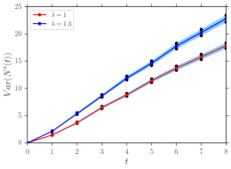
(a)

(b)

Figure 1: $10^{4}$ Monte Carlo simulations of a pure birth process were used to determine the variance of the average depth of a leaf in a random tree, $N^{*}(t)$, and the variance of the average depth of a tree, $G(t)/Z(t)$, where $\lambda$ equals 1 (red lines) and 1.3 (blue lines), and the blue shaded region indicates 95% confidence intervals based on bootstrap percentiles [4, Chapter 13]. (a) Consistent with [16], $\text{Var}\left(N^{*}(t)\right)\sim 2\lambda t$. (b) Consistent with Theorem 1, $\text{Var}\left(G(t)/Z(t)\right)\sim 7$ irrespective of $\lambda$.

2 Results

Before proceeding with the analysis of the two terms on the RHS of (1), we prove a lemma that will simplify the proofs of Lemmas 2 and 3. For that, we introduce a new process, $\{{S}(t)\}$, denoting the sum of the squares of the depths of the leaves at time $t$, which appears when the second moment of $G(t)/Z(t)$ is studied. In the following we also consider the discrete-time process associated with $\{G(t)\}$ and $\{S(t)\}$, namely $\{G_{k}\}$ and $\{{S}_{k}\}$, which account for the sum and the sum of the squares of the depths of the leaves, respectively, when the number of leaves is $k$.

Lemma 1.

We have that

$$\mathbbm{E}\left(\frac{G(t)}{Z(t)}\Big{|}Z(t)=k\right) =\frac{\mathbbm{E}\left(G_{k}\right)}{k}=2\sum_{i=2}^{k}\frac{1}{i},\qquad\qquad\frac{\mathbbm{E}\left({S}_{k}\right)}{k}=4\sum_{i=2}^{k-1}\frac{\mathbbm{E}\left(G_{i}\right)}{i(i+1)}+\frac{\mathbbm{E}\left(G_{k}\right)}{k},$$ (2)

$$\mathbbm{E}\left(\frac{G(t)^{2}}{Z(t)^{2}}\Big{|}Z(t)=k\right) =\frac{\mathbbm{E}\left(G_{k}^{2}\right)}{k^{2}}=\frac{k+1}{k}\left(\sum_{i=1}^{k-1}\frac{\mathbbm{E}\left({S}_{i}\right)}{i(i+1)(i+2)}+4\sum_{i=1}^{k-1}\frac{1}{(i+1)(i+2)}+4\sum_{i=1}^{k-1}\frac{\mathbbm{E}\left(G_{i}\right)}{i(i+2)}\right).$$ (3)

Proof.

Throughout this proof, we condition on $Z(t)=k$ and denote by $\Gamma_{1},\Gamma_{2},\ldots,\Gamma_{k}$ the depth of the $k$ leaves present at time $t$, which are not independent. From the definitions, we have $G_{k}:=\sum_{i=1}^{k}\Gamma_{i}$ and ${S}_{k}:=\sum_{i=1}^{k}\Gamma_{i}^{2}$. The idea of the proof is to recover the formulas given above by finding recurrence equations for $\mathbbm{E}\left(G_{k}\right),\mathbbm{E}\left(S_{k}\right)$, and $\mathbbm{E}\left(G_{k}^{2}\right)$.

For $j\in\{1,2,\ldots,k\}$, denote by $I_{j}$ a random variable that takes value $1$ if the $j$-th leaf is the first one, among the $k$ existing, to extend the tree with two new leaves, and $0$ otherwise. The random variables in the set $\{I_{j},\Gamma_{1},\ldots,\Gamma_{k}\}$ are independent for $j\in\{1,2,\ldots,k\}$ and, due to the memoryless property of the exponential distribution, $\mathbbm{P}\left(I_{j}=1\right)=1/k$ for all $j\in\{1,2,\ldots,k\}$, with $k$ the number of leaves in the tree. Furthermore, the $I_{j}$ are not independent of each other because only one of them can assume value $1$, i.e. $\sum_{j=1}^{k}I_{j}=1$, implying that $I_{j}^{2}=I_{j}$ and $I_{j}I_{\ell}=0$ if $j\neq\ell$. With that in mind, we establish the following relations

$$G_{k+1}=G_{k}+ \sum_{j=1}^{k}I_{j}\Gamma_{j}+2,\qquad\qquad S_{k+1}={S}_{k}+\sum_{j=1}^{k}I_{j}\left(2(\Gamma_{j}+1)^{2}-\Gamma_{j}^{2}\right),$$ (4)

$$G_{k+1}^{2} =G_{k}^{2}+\left(\sum_{j=1}^{k}I_{j}\Gamma_{j}\right)^{2}+4+4G_{k}+4\sum_{j=1}^{k}I_{j}\Gamma_{j}+2G_{k}\sum_{j=1}^{k}I_{j}\Gamma_{j}$$

$$=G_{k}^{2}+\sum_{j=1}^{k}I_{j}\Gamma_{j}^{2}+4+4G_{k}+4\sum_{j=1}^{k}I_{j}\Gamma_{j}+2G_{k}\sum_{j=1}^{k}I_{j}\Gamma_{j}.$$ (5)

From the first equation in (4) we obtain

$$\mathbbm{E}\left(G_{k+1}\right) =\mathbbm{E}\left(G_{k}\right)+\sum_{j=1}^{k}\mathbbm{E}\left(I_{j}\Gamma_{j}\right)+2=\mathbbm{E}\left(G_{k}\right)+\sum_{j=1}^{k}\mathbbm{E}\left(I_{j}\right)\mathbbm{E}\left(\Gamma_{j}\right)+2$$

$$=\mathbbm{E}\left(G_{k}\right)+\frac{1}{k}\mathbbm{E}\left(\sum_{j=1}^{k}\Gamma_{j}\right)+2=\mathbbm{E}\left(G_{k}\right)+\frac{1}{k}\mathbbm{E}\left(G_{k}\right)+2=\frac{k+1}{k}\mathbbm{E}\left(G_{k}\right)+2,$$

where we have used that $I_{j}$ and $\Gamma_{j}$ are independent. This gives the following recurrence relation $\mathbbm{E}\left(G_{k+1}\right)(k+1)^{-1}=\mathbbm{E}\left(G_{k}\right)k^{-1}+2(k+1)^{-1}$, that, solved with initial condition $\mathbbm{E}\left(G_{1}\right)=0$, results in the first formula in (2).

Similarly, using the second equation in (4), we have that

$$\mathbbm{E}\left({S}_{k+1}\right) =\mathbbm{E}\left({S}_{k}\right)+\sum_{j=1}^{k}\mathbbm{E}\left(I_{j}\right)\mathbbm{E}\left(2(\Gamma_{j}+1)^{2}-\Gamma_{j}^{2}\right)=\mathbbm{E}\left({S}_{k}\right)+\frac{1}{k}\sum_{j=1}^{k}\mathbbm{E}\left(\Gamma_{j}^{2}+4\Gamma_{j}+2\right)$$

$$=\mathbbm{E}\left({S}_{k}\right)+\frac{1}{k}\mathbbm{E}\left({S}_{k}\right)+\frac{4}{k}\mathbbm{E}\left(G_{k}\right)+2=\frac{k+1}{k}\mathbbm{E}\left({S}_{k}\right)+\frac{4}{k}\mathbbm{E}\left(G_{k}\right)+2,$$

from which we get the recurrence equation $\mathbbm{E}\left({S}_{k+1}\right)(k+1)^{-1}=\mathbbm{E}\left({S}_{k}\right)k^{-1}+4\mathbbm{E}\left(G_{k}\right)(k(k+1))^{-1}+2(k+1)^{-1}$. Solving this recursion with $\mathbbm{E}\left({S}_{1}\right)=\mathbbm{E}\left(G_{1}\right)=0$, we obtain the second result in (2).

Using (5) and the two results just found (i.e. the formulas in (2)), we can now find an expression for $\mathbbm{E}\left(G_{k}^{2}\right)$.

$$\mathbbm{E}\left(G_{k+1}^{2}\right)= \mathbbm{E}\left(G_{k}^{2}\right)+\frac{1}{k}\sum_{j=1}^{k}\mathbbm{E}\left(\Gamma_{j}^{2}\right)+4+4\mathbbm{E}\left(G_{k}\right)+\frac{4}{k}\sum_{j=1}^{k}\mathbbm{E}\left(\Gamma_{j}\right)+2\mathbbm{E}\left(G_{k}\Big{(}\sum_{j=1}^{k}I_{j}\Gamma_{j}\Big{)}\right)$$

$$= \mathbbm{E}\left(G_{k}^{2}\right)+\frac{1}{k}\mathbbm{E}\left({S}_{k}\right)+4+\left(4+\frac{4}{k}\right)\mathbbm{E}\left(G_{k}\right)+\frac{2}{k}\mathbbm{E}\left(G_{k}\sum_{j=1}^{k}\Gamma_{j}\right)$$

$$= \mathbbm{E}\left(G_{k}^{2}\right)+\frac{\mathbbm{E}\left({S}_{k}\right)}{k}+4+\frac{4(k+1)}{k}\mathbbm{E}\left(G_{k}\right)+\frac{2}{k}\mathbbm{E}\left(G_{k}^{2}\right)$$

$$= \frac{k+2}{k}\mathbbm{E}\left(G_{k}^{2}\right)+\frac{\mathbbm{E}\left({S}_{k}\right)}{k}+4+\frac{4(k+1)}{k}\mathbbm{E}\left(G_{k}\right).$$

The equation above can be rewritten as the recurrence equation

$$\frac{\mathbbm{E}\left(G_{k+1}^{2}\right)}{(k+1)(k+2)}=\frac{\mathbbm{E}\left(G_{k}^{2}\right)}{k(k+1)}+\frac{\mathbbm{E}\left({S}_{k}\right)}{k(k+1)(k+2)}+\frac{4}{(k+1)(k+2)}+\frac{4\mathbbm{E}\left(G_{k}\right)}{k(k+2)},$$

that, when solved with initial condition $\mathbbm{E}\left(G_{1}\right)=\mathbbm{E}\left(G_{1}^{2}\right)=\mathbbm{E}\left({S}_{1}\right)=0$, gives (3). ∎

We now use Lemma 1 to study the limit behaviour of the first term on the RHS of (1).

Lemma 2.

For a pure birth process, we have that

$$\lim_{t\to\infty}\mathbbm{E}\left(\text{Var}\left(\frac{G(t)}{Z(t)}\Big{|}Z(t)\right)\right)=7-\frac{2}{3}\pi^{2}.$$

Proof.

Given that $\lim_{t\to\infty}Z(t)=\infty$ a.s. [6, Chapter 5], for every fixed $k\in\mathbbm{N}$ we have that $\lim_{t\to\infty}\mathbbm{P}\left(Z(t)=k\right)=0$. This implies that

$$\lim_{t\to\infty}\mathbbm{E}\left(\text{Var}\left(\frac{G(t)}{Z(t)}\Big{|}Z(t)\right)\right)=\lim_{t\to\infty}\sum_{k=1}^{\infty}\text{Var}\left(\frac{G_{k}}{k}\Big{|}Z(t)=k\right)\mathbbm{P}\left(Z(t)=k\right)=\lim_{k\to\infty}\text{Var}\left(\frac{G_{k}}{k}\right).$$

Using Lemma 1, we can now compute this variance:

$$\text{Var}\left(\frac{G_{k}}{k}\right) =\frac{\mathbbm{E}\left(G_{k}^{2}\right)}{k^{2}}-\frac{\mathbbm{E}\left(G_{k}\right)^{2}}{k^{2}}$$

$$=\frac{k+1}{k}\bigg{[}\sum_{i=1}^{k-1}\frac{\mathbbm{E}\left({S}_{i}\right)}{i(i+1)(i+2)}+4\sum_{i=1}^{k-1}\frac{1}{(i+1)(i+2)}+4\sum_{i=1}^{k-1}\frac{\mathbbm{E}\left(G_{i}\right)}{i(i+2)}\bigg{]}-\frac{\mathbbm{E}\left(G_{k}\right)^{2}}{k^{2}}$$

$$=\frac{k+1}{k}\bigg{[}\sum_{i=1}^{k-1}\frac{\mathbbm{E}\left({S}_{i}\right)}{i(i+1)(i+2)}+4\sum_{i=1}^{k-1}\frac{1}{(i+1)(i+2)}+4\sum_{i=1}^{k}\frac{\mathbbm{E}\left(G_{i}\right)}{i^{2}}$$

$$\quad+4\sum_{i=1}^{k-1}\Big{(}\frac{\mathbbm{E}\left(G_{i}\right)}{i(i+2)}-\frac{\mathbbm{E}\left(G_{i}\right)}{i^{2}}\Big{)}-4\frac{\mathbbm{E}\left(G_{k}\right)}{k^{2}}\bigg{]}-\frac{\mathbbm{E}\left(G_{k}\right)^{2}}{k^{2}}$$

$$=\frac{k+1}{k}\bigg{[}\sum_{i=1}^{k-1}\frac{\mathbbm{E}\left({S}_{i}\right)}{i(i+1)(i+2)}+4\sum_{i=1}^{k-1}\frac{1}{(i+1)(i+2)}+4\sum_{i=2}^{k}\frac{1}{i^{2}}+\frac{\mathbbm{E}\left(G_{k}\right)^{2}}{k^{2}}$$

$$\quad-8\sum_{i=1}^{k-1}\frac{\mathbbm{E}\left(G_{i}\right)}{i^{2}(i+2)}-4\frac{\mathbbm{E}\left(G_{k}\right)}{k^{2}}\bigg{]}-\frac{\mathbbm{E}\left(G_{k}\right)^{2}}{k^{2}}$$

$$=\frac{k+1}{k}\bigg{[}\sum_{i=1}^{k-1}\frac{\mathbbm{E}\left({S}_{i}\right)}{i(i+1)(i+2)}+4\sum_{i=1}^{k-1}\frac{1}{(i+1)(i+2)}+4\sum_{i=2}^{k}\frac{1}{i^{2}}$$

$$\quad-8\sum_{i=1}^{k-1}\frac{\mathbbm{E}\left(G_{i}\right)}{i^{2}(i+2)}-4\frac{\mathbbm{E}\left(G_{k}\right)}{k^{2}}\bigg{]}+\frac{\mathbbm{E}\left(G_{k}\right)^{2}}{k^{3}},$$

where in the third equality we have added and subtracted the quantity

$$4\sum_{i=1}^{k}\frac{\mathbbm{E}\left(G_{i}\right)}{i^{2}}= 8\sum_{i=2}^{k}\frac{1}{i}\sum_{j=2}^{i}\frac{1}{j}=8\sum_{i=2}^{k}\frac{1}{i^{2}}+8\sum_{i=2}^{k}\sum_{j=2}^{i-1}\frac{1}{ij}$$

$$= 8\sum_{i=2}^{k}\frac{1}{i^{2}}+4\left(\left(\sum_{i=2}^{k}\frac{1}{i}\right)^{2}-\sum_{i=2}^{k}\frac{1}{i^{2}}\right)=4\sum_{i=2}^{k}\frac{1}{i^{2}}+\frac{\mathbbm{E}\left(G_{k}\right)^{2}}{k^{2}}.$$

Taking the limit as $k\to\infty$, we have that

$$\lim_{k\to\infty}\text{Var}\left(\frac{G_{k}}{k}\right)= \sum_{i=1}^{\infty}\frac{\mathbbm{E}\left({S}_{i}\right)}{i(i+1)(i+2)}+4\sum_{i=1}^{\infty}\frac{1}{(i+1)(i+2)}+4\sum_{i=2}^{\infty}\frac{1}{i^{2}}-8\sum_{i=1}^{\infty}\frac{\mathbbm{E}\left(G_{i}\right)}{i^{2}(i+2)}$$

$$= \sum_{i=1}^{\infty}\frac{\mathbbm{E}\left({S}_{i}\right)}{i(i+1)(i+2)}+2+4\Big{(}\frac{\pi^{2}}{6}-1\Big{)}-8\sum_{i=1}^{\infty}\frac{\mathbbm{E}\left(G_{i}\right)}{i^{2}(i+2)}.$$ (6)

Using Lemma 1, the first term on the RHS of (2) becomes

$$\sum_{i=1}^{\infty}\frac{1}{(i+1)(i+2)}\left(4\sum_{k=2}^{i-1}\frac{1}{k+1}\frac{\mathbbm{E}\left(G_{k}\right)}{k}+\frac{\mathbbm{E}\left(G_{i}\right)}{i}\right)\\ =8\sum_{i=1}^{\infty}\frac{1}{(i+1)(i+2)}\sum_{k=2}^{i-1}\frac{1}{k+1}\sum_{j=2}^{k}\frac{1}{j}+2\sum_{i=1}^{\infty}\frac{1}{(i+1)(i+2)}\sum_{k=2}^{i}\frac{1}{k}.$$ (7)

The first term on the RHS of (7) is given by

$$8\sum_{j=2}^{\infty}\frac{1}{j}\sum_{k=j}^{\infty}\frac{1}{k+1}\sum_{i=k+1}^{\infty}\frac{1}{(i+1)(i+2)}=8\sum_{j=2}^{\infty}\frac{1}{j}\sum_{k=j}^{\infty}\frac{1}{k+1}\frac{1}{k+2}=8\sum_{j=2}^{\infty}\frac{1}{j}\frac{1}{j+1}=4,$$

whereas the second one is given by

$$2\sum_{k=2}^{\infty}\frac{1}{k}\sum_{i=k}^{\infty}\frac{1}{(i+1)(i+2)}=2\sum_{k=2}^{\infty}\frac{1}{k}\frac{1}{k+1}=1.$$

So, the first sum in the RHS of (2) is equal to $4+1=5$. For the last sum in the RHS of (2), we have

$$-8\sum_{i=1}^{\infty}\frac{1}{i(i+2)}\frac{\mathbbm{E}\left(G_{i}\right)}{i} =-16\sum_{i=1}^{\infty}\frac{1}{i(i+2)}\sum_{j=2}^{i}\frac{1}{j}=-16\sum_{j=2}^{\infty}\frac{1}{j}\sum_{i=j}^{\infty}\frac{1}{i(i+2)}$$

$$=-16\sum_{j=2}^{\infty}\frac{1}{j}\frac{1+2j}{2j(j+1)}=-\frac{4}{3}(\pi^{2}-3).$$

Joining all these results, we obtain

$$\lim_{k\to\infty}\text{Var}\left(\frac{G_{k}}{k}\right)=5+2+4\Big{(}\frac{\pi^{2}}{6}-1\Big{)}-\frac{4}{3}(\pi^{2}-3)=7-\frac{2}{3}\pi^{2}.$$

∎

Lemma 1 allows us to also understand the behaviour of the conditional variance of the expected average depth of the leaves given their number.

Lemma 3.

For a pure birth process, we have that

$$\lim_{t\to\infty}\text{Var}\left(\mathbbm{E}\left(\frac{G(t)}{Z(t)}|Z(t)\right)\right)=\frac{2}{3}\pi^{2}\approx 6.58.$$

Proof.

From Lemma 1 we know that

$$\text{Var}\left(\mathbbm{E}\left(\frac{G(t)}{Z(t)}|Z(t)\right)\right) =\text{Var}\left(2\sum_{i=2}^{Z(t)}\frac{1}{i}\right)=4\text{Var}\left(\sum_{i=1}^{Z(t)}\frac{1}{i}\right)=4\left(\mathbbm{E}\left(\left(\sum_{i=1}^{Z(t)}\frac{1}{i}\right)^{2}\right)-\left(\mathbbm{E}\left(\sum_{i=1}^{Z(t)}\frac{1}{i}\right)\right)^{2}\right),$$ (8)

where, in the second inequality, we have used the fact that the variance of a process doesn’t change when a constant is added. Given that $\{Z(t)\}$ is a pure birth process, the distribution of $Z(t)$ is given by (e.g. [14, pg. 430])

$$\mathbbm{P}\left(Z(t)=k\right)=e^{-\lambda t}(1-e^{-\lambda t})^{k-1},\quad k=1,2,\ldots$$

where $1/\lambda$ is the expected time before a leaf generates two new leaves, which allows us to evaluate the second term in (8) exactly:

$$\mathbbm{E}\left(\sum_{i=1}^{Z(t)}\frac{1}{i}\right) =\sum_{k=1}^{\infty}{\mathbbm{P}}(Z(t)=k)\sum_{i=1}^{k}\frac{1}{i}=\frac{e^{-\lambda t}}{1-e^{-\lambda t}}\sum_{k=1}^{\infty}(1-e^{-\lambda t})^{k}\sum_{i=1}^{k}\frac{1}{i}$$

$$=\frac{e^{-\lambda t}}{1-e^{-\lambda t}}\sum_{i=1}^{\infty}\frac{1}{i}\sum_{k=i}^{\infty}(1-e^{-\lambda t})^{k}=\frac{1}{(1-e^{-\lambda t})}\sum_{i=1}^{\infty}\frac{1}{i}(1-e^{-\lambda t})^{i}.$$

Let $f(t):=\sum_{i=1}^{\infty}(1-e^{-\lambda t})^{i}/i$. Then

$$f^{\prime}(t)=\lambda e^{-\lambda t}\sum_{i=1}^{\infty}\frac{1}{i}i(1-e^{-\lambda t})^{i-1}=\lambda e^{-\lambda t}\sum_{i=1}^{\infty}(1-e^{-\lambda t})^{i-1}=\lambda,$$

and, given $f(0)=0$, we have that $f(t)=\lambda t$. This implies that

$$\mathbbm{E}\left(\sum_{i=1}^{Z(t)}\frac{1}{i}\right)=\frac{\lambda t}{(1-e^{-\lambda t})}=\lambda t+o(1),$$ (9)

and the second term in the brackets on the RHS of (8) is therefore $(\lambda^{2}t^{2})/(1-e^{-\lambda t})^{2}$.

Consider the first term on the RHS of (8).

$$\mathbbm{E}\left(\left(\sum_{i=1}^{Z(t)}\frac{1}{i}\right)^{2}\right) =\frac{e^{-\lambda t}}{1-e^{-\lambda t}}\sum_{i=1}^{\infty}\left(\sum_{k=1}^{i}\frac{1}{k}\right)^{2}(1-e^{-\lambda t})^{i}$$

$$=\frac{e^{-\lambda t}}{1-e^{-\lambda t}}\left(\sum_{i=1}^{\infty}\sum_{k=1}^{i}\frac{1}{k^{2}}(1-e^{-\lambda t})^{i}+2\sum_{i=1}^{\infty}\sum_{k=1}^{i}\sum_{j=1}^{k-1}\frac{1}{k}\frac{1}{j}(1-e^{-\lambda t})^{i}\right).$$ (10)

The first term in the brackets on the RHS of (2) is given by

$$\sum_{i=1}^{\infty}\sum_{k=1}^{i}\frac{1}{k^{2}}(1-e^{-\lambda t})^{i}=\sum_{k=1}^{\infty}\sum_{i=k}^{\infty}\frac{1}{k^{2}}(1-e^{-\lambda t})^{i}=e^{\lambda t}\sum_{k=1}^{\infty}\frac{1}{k^{2}}(1-e^{-\lambda t})^{k}.$$

For the second term, we have that

$$2\sum_{i=1}^{\infty}\sum_{k=1}^{i}\sum_{j=1}^{k-1}\frac{1}{k}\frac{1}{j}(1-e^{-\lambda t})^{i}=2\sum_{k=1}^{\infty}\sum_{j=1}^{k-1}\sum_{k=i}^{\infty}\frac{1}{k}\frac{1}{j}(1-e^{-\lambda t})^{i}=2e^{\lambda t}\sum_{k=1}^{\infty}\sum_{j=1}^{k-1}\frac{1}{k}\frac{1}{j}(1-e^{-\lambda t})^{k}.$$

Denoting with $g(t):=2\sum_{k=1}^{\infty}\sum_{j=1}^{k-1}(1-e^{-\lambda t})^{k}/(kj)$ and noticing that $g(0)=0$ and

$$g^{\prime}(t) =\frac{2\lambda e^{-\lambda t}}{1-e^{-\lambda t}}\sum_{k=1}^{\infty}\sum_{j=1}^{k-1}\frac{1}{j}(1-e^{-\lambda t})^{k}=\frac{2\lambda e^{-\lambda t}}{1-e^{-\lambda t}}\sum_{j=1}^{\infty}\sum_{k=j+1}^{\infty}\frac{1}{j}(1-e^{-\lambda t})^{k}$$

$$=\frac{2\lambda}{1-e^{-\lambda t}}\sum_{j=1}^{\infty}\frac{1}{j}(1-e^{-\lambda t})^{j+1}=2\lambda f(t)=2\lambda^{2}t,$$

we obtain that $g_{2}(t)=\lambda^{2}t^{2}$, and the second term on the RHS of (2) is thus $(\lambda^{2}t^{2})/(1-e^{-\lambda t})$.

So, joining all the results, we have that

$$\lim_{t\to\infty}\text{Var}\left(\mathbbm{E}\left(\frac{G(t)}{Z(t)}|Z(t)\right)\right)=\lim_{t\to\infty}4\left(\sum_{k=1}^{\infty}\frac{(1-e^{-\lambda t})^{k-1}}{k^{2}}+\frac{\lambda^{2}t^{2}}{1-e^{-\lambda t}}-\frac{\lambda^{2}t^{2}}{(1-e^{-\lambda t})^{2}}\right)=4\sum_{k=1}^{\infty}\frac{1}{k^{2}}=\frac{2}{3}\pi^{2}$$

∎

Theorem 1 follows from equation (1) using the results in Lemmas 2 and 3.

Acknowledgments: The authors thank Tom S. Weber (WEHI) for contributing to the conjecture of Theorem 1. Part of this work was supported by Science Foundation Ireland grant 12 IP 1263.

References

• [1] J. D. Biggins and D. R. Grey. A note on the growth of random trees. Stat. Probab. Lett., 32(4):339–342, 1997.
• [2] J. K. Blitzstein and J. Hwang. Introduction to probability. Chapman and Hall/CRC, 2014.
• [3] L. Devroye. A note on the height of binary search trees. J. ACM, 33(3):489–498, 1986.
• [4] B. Efron and R. J. Tibshirani. An introduction to the bootstrap. CRC press, 1994.
• [5] P. Flajolet and A. Odlyzko. Exploring binary trees and other simple trees. In 21st FOCS, pages 207–216. IEEE, 1980.
• [6] T. E. Harris. The theory of branching processes. Springer-Verlag, Berlin, 1963.
• [7] P. Jagers. Renewal theory and the almost sure convergence of branching processes. Ark. Mat., 7(6):495–504, 1969.
• [8] M. Kimmel and D. E. Axelrod. Branching Processes in Biology. Springer, 2002.
• [9] J. M. Marchingo, G. Prevedello, A. J. Kan, S. Heinzel, P. D. Hodgkin, and K. R. Duffy. T cell stimuli independently sum to regulate an inherited clonal division fate. Nat. Commun., 7:13540, 2016.
• [10] G. Meli, T. S. Weber, and K. R. Duffy. Sample path properties of the average generation of a Bellman-Harris process. arXiv 1807.07031, 2018.
• [11] L. Perié, P. D. Hodgkin, S. H. Naik, T. N. Schumacher, R. J. de Boer, and K. R. Duffy. Determining lineage pathways from cellular barcoding experiments. Cell Rep., 6(4):617–624, 2014.
• [12] B. Pittel. On growing random binary trees. J. Math. Anal. Appl., 103(2):461–480, 1984.
• [13] B. Pittel. Note on the heights of random recursive trees and random m-ary search trees. Random Struct. Algor., 5(2):337–347, 1994.
• [14] S. I. Resnick. Adventures in stochastic processes. Springer Science & Business Media, 2013.
• [15] J. M. Robson. The height of binary search trees. Aust. Comput. J., 11(4):151–153, 1979.
• [16] M. L. Samuels. Distribution of the branching-process population among generations. J. Appl. Prob., 8(04):655–667, 1971.
• [17] T. S. Weber, L. Perié, and K. R. Duffy. Inferring average generation via division-linked labeling. J. Math. Bio., 73(2):491–523, 2016.