A Study on Optimal Beam Patterns for Single User Massive MIMO Transmissions

Summary

This paper proposes optimal beam patterns of analog beamforming for SU (Single User) massive MIMO (Multi-Input Multi-Output) transmission systems. For hybrid beamforming in SU massive MIMO systems, there are several design parameters such as beam patterns, the number of beams (streams), the shape of array antennas, and so on. In conventional hybrid beamforming, rectangular patch array antennas implemented on a planar surface with linear phase shift beam patterns have been used widely. However, it remains unclear whether existing configurations are optimal or not. Therefore, we propose a method using OBPB (Optimal Beam Projection Beamforming) for designing configuration parameters of the hybrid beamforming. By using the method, the optimal beam patterns are derived first, and are projected on the assumed surface to calculate the achievable number of streams and the resulting channel capacity. The results indicate OBPB with a spherical surface yields at least 3.5 times higher channel capacity than conventional configurations.

keywords: massive MIMO, beamforming, beam pattern, directivity, spherical mode expansion, capacity maximization.

1 Introduction

Future wireless communication systems must offer larger channel capacity because of the popularization of wireless devices such as smartphones and tablets. To increase the channel capacity, massive MIMO (Multi-Input Multi-Output) technology using a large number of antenna elements, at least at the BS (Base Station), is important [1, 2], and the technology is expected to be deployed in 5G cellular networks and beyond. In the case of MU (Multi-User) massive MIMO, the channel (system) capacity increases in proportion to the number of antenna elements if UEs (User Equipment) are well separated in space [3]. However, in the case of SU (Single User) massive MIMO, this is not true and the number of streams for spatial multiplexing is limited due to both smaller antenna surface at the UE and the increased antenna correlation at the BS.

Hybrid beamforming, which combines analog beamforming and digital pre/post-processing, is a reasonable way to realize massive MIMO systems in low cost and low power consumption [4, 7, 5, 6]. In conventional hybrid beamforming, rectangular patch array antennas implemented on a planar surface with linear phase shift beam patterns have been used widely [8, 9]. In the case of MU massive MIMO with UEs well separated in the space, it works well by just steering main beams to locations (angles seen from the BS) of the UEs. However, in the case of SU massive MIMO, it will not work well since steering main beams to the single UE is just increasing antenna correlation at the BS. Therefore, there are remaining research issues in the case of SU massive MIMO in terms of beam patterns, the number of beams (streams), the shape of an array antenna, and so on.

In this paper, we introduce a method using OBPB (Optimal Beam Projection Beamforming) proposed in [10] for designing antenna configuration parameters of the SU massive MIMO. The goal of the study is to maximize channel capacity by increasing the effective number of beams (streams) in a given propagation channel with special beam patterns and shapes of antenna designed by the OBPB. Different from the conventional design methods, the OBPB derives optimal beam patterns to be matched with the propagation channel first, and projects the optimal beam patterns to the assumed antenna surface such as sphere to synthesize conditional beam patterns. In the method that we proposed, the optimal solutions of the transmit and receive sides are derived by sequential calculations on a computer. Thus, there is no information exchanged between BS and UE. The necessary information to derive the solutions is only the joint angular profile to make the corresponding antenna radiation patterns for usage. Thus, only measurements and feedbacks to determine the joint angular profile are required without any other information exchanges to calculate the optimal patterns even in real operation. Since OBPB utilizes as much space of the antenna surface as possible, the larger number of orthogonal beams (streams) can be created. Table 1 compares the antenna configuration and metrics of OBPB with those of conventional methods for the analog beamforming. From the analysis, it is found that the channel capacity realized by the OBPB with a spherical surface approaches the optimal capacity and is 3.5 times or larger than that of the conventional configurations.

This paper is organized as follows. In Sect. 2, system model of SU massive MIMO and antenna configuration of the conventional hybrid beamforming are described. In Sect. 3, the proposed method using OBPB is introduced to design conditionally optimal antenna configuration parameters. Section 4 designs conditionally optimal beam patterns in a given environment and calculate the achievable number of streams and the resulting channel capacity with deep discussions about the results. Finally, Sect. 5 concludes this paper.

Table 1: Analog beamforming configuration.

	Conventional	Proposed
Shape	Planar	Spherical, Planar
Category	Full-array, Sub-array	Hemisphere, 1/32-sphere, Plane
Beamforming	Linear Phase Shift Beamforming (LPSB)	Optimal Beam Projection Beamforming (OBPB) [10]
Antenna type	Patch array	Continuous surface
Beam selection metric	Received power, Determinant	Determinant
Rank adaptation metric	Capacity	Capacity

2 Conventional hybrid beamforming for SU-massive MIMO system

There are two categories of configurations, such as full-array and sub-array in the conventional hybrid beamforming for the SU-massive MIMO. The antenna elements are considered as the rectangular patch array antennas implemented on a planar surface with LPSB (Linear Phase Shift Beamforming). The beam patterns are selected to maximize the received power of each stream or to maximize the determinant of a channel correlation matrix by using a combinatorial search.

2.1 SU-massive MIMO system model

The massive MIMO system is achieved by using dozens, hundreds or more antenna elements at least at the BS to improve channel (system) capacity as shown in Fig. 1. In the massive MIMO system, combining analog beamforming and digital pre/post-processing is a reasonable way for low cost and low power consumption. It is called as hybrid beamforming and its procedure consists of long-term and short-term operations as shown in Fig. 2.

The receive uplink signals of $M$ streams in the SU-massive MIMO system at time $t$ is defined as

$$\mathbf{y}_{\mathrm{BS}}(t) =\mathbf{W}_{\mathrm{d}}^{\mathrm{T}}(t)\mathbf{W}_{\mathrm{a}}^{\mathrm{T}}\mathbf{H}_{0}(t)\mathbf{s}_{\mathrm{UE}}(t)+\mathbf{n}_{\mathrm{BS}}(t)$$

$$=\mathbf{W}_{\mathrm{d}}^{\mathrm{T}}(t)\mathbf{H}(t)\mathbf{s}_{\mathrm{UE}}(t)+\mathbf{n}_{\mathrm{BS}}(t)$$ (1)

$$\mathbf{H}(t) =\mathbf{W}_{\mathrm{a}}^{\mathrm{T}}\mathbf{H}_{0}(t),$$ (2)

where $\mathbf{W}_{\mathrm{d}}(t)\!\in\!\mathbb{C}^{M\times M}$ is a digital pre/post-processing weight matrix, $\mathbf{W}_{\mathrm{a}}\!\in\!\mathbb{C}^{N_{\mathrm{BS}}\times M}$ is an analog beamforming weight matrix, $\mathbf{s}_{\mathrm{UE}}\!\in\!\mathbb{C}^{N_{\mathrm{UE}}\times 1}$ is a vector of transmit signal and $\mathbf{n}_{\mathrm{BS}}\!\in\!\mathbb{C}^{M\times 1}$ is a noise vector. $\mathbf{H}_{0}(t)$ is a channel matrix and its component is defined by a channel response between the $i$-th BS antenna and the $j$-th UE antenna $h_{0,ij}$. $\mathbf{H}(t)$ is a channel matrix including the analog beamforming weight matrix. $M$ is the number of streams defined as $M\leq\min\{N_{\mathrm{BS}},N_{\mathrm{UE}}\}$ and $N_{\mathrm{BS}},N_{\mathrm{UE}}$ are the numbers of BS and UE antennas respectively. In this paper, it is assumed that the transmit power is divided equally for all streams. Under the equally distributed power condition, the instantaneous channel capacity is derived as follows.

$$C(t) =\log_{2}\mathrm{det}\left(\mathbf{I}_{M}+\mathbf{W}_{\mathrm{d}}^{\mathrm{T}}(t)\mathbf{H}(t)\mathbf{H}^{\mathrm{H}}(t)\mathbf{W}_{\mathrm{d}}^{\mathrm{*}}(t)\frac{P}{MP_{\mathrm{n}}}\right),$$ (3)

where $\mathbf{I}_{M}$ is an $M\times M$ unity matrix, $P$ is the transmit power and $P_{\mathrm{n}}$ is the noise power. When an SVD (Singular Value Decomposition) is considered, the digital signal processing weight matrix is unitary. Thus, the channel capacity is expressed as

$$C(t) =\log_{2}\mathrm{det}\left(\mathbf{I}_{M}+\mathbf{H}(t)\mathbf{H}^{\mathrm{H}}(t)\frac{P}{MP_{\mathrm{n}}}\right).$$ (4)

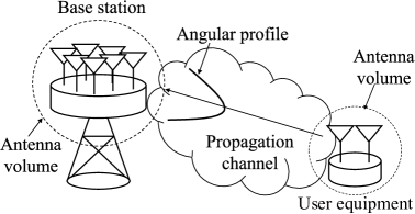
Figure 1: SU-massive MIMO system model.

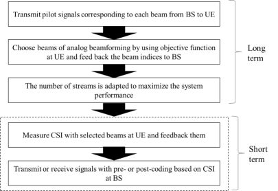
Figure 2: Hybrid beamforming procedure of massive MIMO system.

2.2 Antenna configuration for hybrid beamforming

There are mainly two types of massive MIMO antenna configurations, i.e. the full-array and sub-array as shown in Fig. 3. In the configurations, phase shifters are used to achieve analog beamforming weights. In the case of the full-array configuration, each RF chain is connected to all antenna elements. The weight vector between the $m$-th RF chain and $N_{\mathrm{BS}}$ antenna elements is given by

$$\mathbf{w}_{\mathrm{a},m}=[w_{\mathrm{a},1m},\cdots,w_{\mathrm{a},N_{\mathrm{BS}}m}]^{\mathrm{T}}.$$ (5)

The analog beamforming weight matrix for the full-array configuration is expressed as

$$\mathbf{W}_{\mathrm{a}}=[\mathbf{w}_{\mathrm{a},1},\cdots,\mathbf{w}_{\mathrm{a},M}].$$ (6)

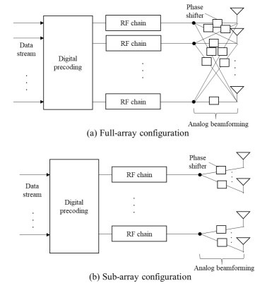
Figure 3: Hybrid beamforming antenna configuration.

On the other hand, in the sub-array configuration, the antennas are divided into several groups and each RF chain is connected to a sub-array group with $N_{\mathrm{BS,sub}}$ antenna elements, defined as $N_{\mathrm{BS,sub}}=N_{\mathrm{BS}}/M=N_{\mathrm{BS,sub,V}}\times N_{\mathrm{BS,sub,H}}$ sub-array antenna elements in order to simplify the feeding circuit. The weight vector between the $m$-th RF chain and $N_{\mathrm{BS,sub}}$ antenna elements is given by

$$\mathbf{w}_{\mathrm{a},m}=[w_{\mathrm{a},1m},\cdots,w_{\mathrm{a},N_{\mathrm{BS,sub}}m}]^{\mathrm{T}}.$$ (7)

The analog beamforming weight matrix for the sub-array configuration is expressed as

$$\mathbf{W}_{\mathrm{a}}=\left[\begin{array}[]{cccc}\mathbf{w}_{\mathrm{a},1}&\mathbf{0}&\cdots&\mathbf{0}\\ \mathbf{0}&\mathbf{w}_{\mathrm{a},2}&&\vdots\\ \vdots&&\ddots&\mathbf{0}\\ \mathbf{0}&\cdots&\mathbf{0}&\mathbf{w}_{\mathrm{a},M}\\ \end{array}\right].$$ (12)

2.3 Analog beamforming weight matrix by using LPSB

When the linear phase shift beam patterns are used for the analog beamforming, the weight matrix is expressed based on a DFT (Discrete Fourier Transform) matrix $\mathbf{D}\!\in\!\mathbb{C}^{N_{\mathrm{BS}}\times a^{2}N_{\mathrm{BS}}}$, where $a$ is a beam interval coefficient determined by an integer. For example, it is assumed in Fig. 5 that 2-dimensional $N_{\mathrm{BS,V}}\times N_{\mathrm{BS,H}}$ rectangular array is used for the full-array. The weight component for the $n=(u,v)$-th antenna element with the phase shifter corresponding to the $m=(p,q)$-th beam pattern is expressed as follows.

$$d_{nm}=d_{up}d_{vq} =\frac{1}{\sqrt{N_{\mathrm{BS}}}}\exp\left(\frac{-j2\pi(u-1)(p-1)}{aN_{\mathrm{BS,V}}}\right)$$

$$\cdot\exp\left(\frac{-j2\pi(v-1)(q-1)}{aN_{\mathrm{BS,H}}}\right),$$ (13)

where $u,v$ are the row indices of the DFT matrix in $\{1,\cdots,N_{\mathrm{BS,V}}\}$ and $\{1,\cdots,N_{\mathrm{BS,H}}\}$ respectively. $p,q$ are the column indices of the DFT matrix in $\{1,\cdots,aN_{\mathrm{BS,V}}\}$ and $\{1,\cdots,aN_{\mathrm{BS,H}}\}$. When the value $a$ becomes large, the main lobes of the beams become near.

In the case of the sub-array as shown in Fig. 5, the weight component for the $n=(u,v)$-th antenna element with the phase shifter corresponding to the $m=(p,q)$-th beam pattern is also expressed as

$$d_{nm}=d_{up}d_{vq} =\frac{1}{\sqrt{N_{\mathrm{BS,sub}}}}\exp\left(\frac{-j2\pi(u-1)(p-1)}{aN_{\mathrm{BS,sub,V}}}\right)$$

$$\cdot\exp\left(\frac{-j2\pi(v-1)(q-1)}{aN_{\mathrm{BS,sub,H}}}\right),$$ (14)

where the indices $u,v$ are integers in $\{1,\cdots,N_{\mathrm{BS,sub,V}}\}$ and $\{1,\cdots,N_{\mathrm{BS,sub,H}}\}$ corresponding to the row indices of the DFT matrix. and the indices $p,q$ are integers in $\{1,\cdots,aN_{\mathrm{BS,sub,V}}\}$ and $\{1,\cdots,aN_{\mathrm{BS,sub,H}}\}$ corresponding to the column indices of the DFT matrix.

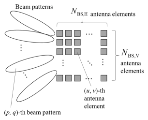
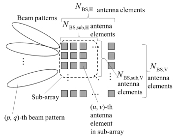
Figure 4: 2-dimensional rectangular full-array configuration.

Figure 5: 2-dimensional rectangular sub-array configuration.

2.4 Beam selection using received power of each stream

We consider two methods for selecting analog beamforming weights. First, the analog beamforming weight vectors are chosen to maximize the received power of each stream. Next, the weight is selected to be descending order of the achievable received power of the stream.

$$\mathbf{w}_{m} =\mathop{\rm arg~{}max}\limits_{\mathbf{d}_{m^{\prime}}\in\mathbf{D}\backslash\mathbf{W}_{m-1}}\mathrm{E}[\mathbf{d}_{m^{\prime}}^{\mathrm{T}}\mathbf{H}(t)\mathbf{H}^{\mathrm{H}}(t)\mathbf{d}_{m^{\prime}}^{\mathrm{*}}]$$ (15)

$$\mathbf{W}_{m-1} =[\mathbf{w}_{1},\cdots,\mathbf{w}_{m-1}],$$ (16)

where $\mathbf{d}_{m^{\prime}}$ is the $m^{\prime}$-th column vector of the matrix $\mathbf{D}$. This method is simple because the only BS or UE side’s information is needed for the calculation. However, the channel capacity degrades due to high correlation between the selected beams made by analog beamforming in this method.

2.5 Beam selection using determinant of channel correlation matrix

Since the analog weight matrix is deterministic, the optimal values are derived by using not the instantaneous channel capacity but the average channel capacity. When $\frac{P_{\mathrm{t}}}{MP_{\mathrm{n}}}$ is sufficiently large, the average channel capacity is given by

$$\bar{C} =\mathrm{E}[C(t)]$$

$$=\log_{2}\mathrm{det}\left(\mathrm{E}\left[\mathbf{I}_{M}+\mathbf{H}(t)\mathbf{H}^{\mathrm{H}}(t)\right]\frac{P}{MP_{\mathrm{n}}}\right)$$

$$\approx\log_{2}\mathrm{det}\left(\mathrm{E}\left[\mathbf{H}(t)\mathbf{H}^{\mathrm{H}}(t)\right]\frac{P_{\mathrm{t}}}{MP_{\mathrm{n}}}\right)$$

$$\propto\mathrm{det}\mathrm{E}\left[\mathbf{H}(t)\mathbf{H}^{\mathrm{H}}(t)\right],$$ (17)

Therefore, to maximize the average channel capacity is equivalent to maximize the determinant of the channel correlation matrix.

$$\mathbf{w}_{m} =\mathop{\rm arg~{}max}\limits_{\mathbf{d}_{m^{\prime}}\in\mathbf{D}\backslash\mathbf{W}_{m-1}}\mathrm{det}\left(\mathrm{E}[\tilde{\mathbf{W}}_{mm^{\prime}}^{\mathrm{T}}\mathbf{H}(t)\mathbf{H}^{\mathrm{H}}(t)\tilde{\mathbf{W}}_{mm^{\prime}}^{\mathrm{*}}]\right)$$ (18)

$$\mathbf{W}_{m-1} =[\mathbf{w}_{1},\cdots,\mathbf{w}_{m-1}]$$ (19)

$$\tilde{\mathbf{W}}_{mm^{\prime}} =[\mathbf{w}_{1},\cdots,\mathbf{w}_{m-1},\mathbf{d}_{m^{\prime}}].$$ (20)

By using this method, the weights can be derived considering both the maximization of the beam gain and the reduction of correlation between the selected beams. Therefore, the channel capacity can be improved compared to the first method using the received power.

3 Analog beamforming by using OBPB

OBPB is used to derive the effective number of beams (streams) and beam patterns and described by using the system model based on an SME (Spherical Mode Expansion) [11]. By using OBPB, optimal beam patterns are derived first to maximize the average channel capacity with the given propagation channel. After that, semi-optimal beam patterns are calculated under a given condition of antenna surface. In this section, we introduce how to derive the semi-optimal beam patterns by projecting the optimal beam patterns to the assumed antenna surface and synthesizing the conditional beam patterns radiated from the surface.

3.1 SU-massive MIMO system model with SME

The channel matrix is expressed by using BS and UE antenna directivities as follows.

$$\mathbf{H}(t)$$

$$=\int_{\psi_{\mathrm{BS}}}\!\int_{\psi_{\mathrm{UE}}}\!\vec{\mathbf{g}}_{\mathrm{BS}}(\psi_{\mathrm{BS}})\vec{\vec{h}}(\psi_{\mathrm{UE}},\psi_{\mathrm{BS}},t)\vec{\mathbf{g}}_{\mathrm{UE}}(\psi_{\mathrm{UE}})\mathrm{d}\psi_{\mathrm{UE}}\mathrm{d}\psi_{\mathrm{BS}}$$

$$=\mathbf{Q}_{\mathrm{BS},M}^{\mathrm{T}}\int_{\psi_{\mathrm{BS}}}\!\int_{\psi_{\mathrm{UE}}}\!\vec{\mathbf{k}}_{\mathrm{BS}}(\psi_{\mathrm{BS}})\vec{\vec{h}}(\psi_{\mathrm{UE}},\psi_{\mathrm{BS}},t)$$

$$\ \ \ \ \ \ \vec{\mathbf{k}}_{\mathrm{UE}}(\psi_{\mathrm{UE}})\mathrm{d}\psi_{\mathrm{UE}}\mathrm{d}\psi_{\mathrm{BS}}\mathbf{Q}_{\mathrm{UE},M}^{*}$$ (21)

$$\vec{\mathbf{g}}_{\mathrm{BS}}(\psi_{\mathrm{BS}})=\mathbf{Q}_{\mathrm{BS},M}^{\mathrm{T}}\vec{\mathbf{k}}_{\mathrm{BS}}(\psi_{\mathrm{BS}})$$ (22)

$$\vec{\mathbf{g}}_{\mathrm{UE}}(\psi_{\mathrm{UE}})=\mathbf{Q}_{\mathrm{UE},M}^{\mathrm{T}}\vec{\mathbf{k}}_{\mathrm{UE}}(\psi_{\mathrm{UE}}),$$ (23)

where the departure or arrival angles at BS and UE are $\psi_{\mathrm{BS}}=(\theta_{\mathrm{BS}},\phi_{\mathrm{BS}})$ in a spherical coordinate shown in Fig. 6. And $\psi_{\mathrm{UE}}=(\theta_{\mathrm{UE}},\phi_{\mathrm{UE}})$. $\mathbf{Q}_{\mathrm{BS},M}\!\in\!\mathbb{C}^{J_{\mathrm{BS}}\times M},\mathbf{Q}_{\mathrm{UE},M}\!\in\!\mathbb{C}^{J_{\mathrm{UE}}\times M}$ are matrices of spherical mode coefficients which determine the beam patterns for $M$ streams. $J_{\mathrm{BS}}$ and $J_{\mathrm{UE}}$ are numbers of the spherical modes. $\vec{\mathbf{k}}_{\mathrm{BS}}(\psi_{\mathrm{BS}})\!\in\!\mathbb{C}^{J_{\mathrm{BS}}\times 1},\vec{\mathbf{k}}_{\mathrm{UE}}(\psi_{\mathrm{UE}})\!\in\!\mathbb{C}^{J_{\mathrm{UE}}\times 1}$ are vectors of far-field pattern functions which are canonical solutions of Helmholtz equation.

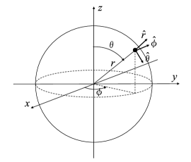
Figure 6: Spherical coordinate.

Figure 7: MIMO system model with SME.

From Eq. (2.5), the maximization of the average channel capacity is equal to that of the determinant of the channel correlation matrix. When SME is used, the channel correlation matrix which transmits and receives $M$ streams is expressed as follows.

$$\mathbf{R}_{\mathrm{BS,h}} =\mathrm{E}[\mathbf{H}(t)\mathbf{H}^{\mathrm{H}}(t)]$$

$$=\int_{\psi_{\mathrm{BS}}}\int_{\psi_{\mathrm{UE}}}\vec{\mathbf{g}}_{\mathrm{BS}}(\psi_{\mathrm{BS}})\cdot\Big{(}\vec{\mathbf{g}}^{\mathrm{T}}_{\mathrm{UE}}(\psi_{\mathrm{UE}})\cdot\vec{\vec{P}}_{\mathrm{h}}(\psi_{\mathrm{BS}},\psi_{\mathrm{UE}})$$

$$\cdot\vec{\mathbf{g}}^{*}_{\mathrm{UE}}(\psi_{\mathrm{UE}})\Big{)}\cdot\vec{\mathbf{g}}^{\mathrm{H}}_{\mathrm{BS}}(\psi_{\mathrm{BS}})\mathrm{d}\psi_{\mathrm{UE}}\mathrm{d}\psi_{\mathrm{BS}}$$

$$=\int_{\psi_{\mathrm{BS}}}\mathbf{Q}_{\mathrm{BS}}^{\mathrm{T}}\vec{\mathbf{k}}_{\mathrm{BS}}(\psi_{\mathrm{BS}})\cdot\vec{P}_{\mathrm{h,BS}}(\psi_{\mathrm{BS}})$$

$$\cdot\vec{\mathbf{k}}^{\mathrm{H}}_{\mathrm{BS}}(\psi_{\mathrm{BS}})\mathbf{Q}_{\mathrm{BS}}^{\mathrm{*}}\mathrm{d}\psi_{\mathrm{BS}}.$$ (24)

$\vec{\vec{P}}_{\mathrm{h}}(\psi_{\mathrm{BS}},\psi_{\mathrm{UE}})$ is a joint angular profile, which is the time-averaged power of the channel response from a certain departure angle to a certain arrival angle. $\vec{P}_{\mathrm{h,BS}}(\psi_{\mathrm{BS}})$ is a marginal angular profile at BS, which is determined by the channel response and the beam patterns of UE antennas. These angular profiles are defined as follows.

$$\vec{\vec{P}}_{\mathrm{h}}(\psi_{\mathrm{BS}},\psi_{\mathrm{UE}})=\mathrm{E}\bigg{[}\left|\vec{\vec{h}}(\psi_{\mathrm{BS}},\psi_{\mathrm{UE}},t)\right|^{2}\bigg{]}$$ (25)

$$\vec{P}_{\mathrm{h,BS}}(\psi_{\mathrm{BS}})$$

$$=\int_{\psi_{\mathrm{UE}}}\vec{\vec{P}}_{\mathrm{h}}(\psi_{\mathrm{BS}},\psi_{\mathrm{UE}})\cdot\vec{\mathbf{g}}^{\mathrm{T}}_{\mathrm{UE}}(\psi_{\mathrm{UE}})\cdot\vec{\mathbf{g}}_{\mathrm{UE}}^{*}(\psi_{\mathrm{UE}})\mathrm{d}\psi_{\mathrm{UE}}.$$ (26)

At the UE side, the channel correlation matrix is expressed in the same way at the BS.

3.2 Iterative beam pattern optimization

By using the SU-massive MIMO system model with SME, we obtain the optimal beam patterns of BS and UE. The optimization method described in [10] is expanded in the case of the different antenna volume at BS and UE. Since the beam patterns are determined by the spherical mode coefficients (SMCs) , we introduce the optimization method of SMCs of BS and UE. In the method, the analog beamforming weights and beam patterns of antenna elements are considered as a matrix of SMCs and far-field pattern functions. The determinant of the channel correlation matrix can be maximized by controlling the matrix of SMCs $\mathbf{Q}_{\mathrm{BS},M}$. Since the channel correlation matrix is semi-positive definite matrix, it can be transformed by the eigenvalue decomposition using the matrix of SMCs. The maximum determinant of the channel correlation matrix is expressed as follows.

$$\max\det\mathbf{R}_{\mathrm{BS,h}}=\max\det(\mathbf{Q}^{\mathrm{T}}_{\mathrm{BS},M}\mathbf{R}_{\mathrm{BS,sph}}\mathbf{Q}^{*}_{\mathrm{BS},M})$$

$$=\prod_{j=1}^{M}(\mathbf{u}^{\mathrm{H}}_{\mathrm{BS}j}\mathbf{R}_{\mathrm{BS,sph}}\mathbf{u}_{\mathrm{BS}j})=\prod_{j=1}^{M}\lambda_{\mathrm{BS}j},$$ (27)

where $\mathbf{u}_{\mathrm{BS}j}$ is an eigenvector and $\lambda_{\mathrm{BS}j}(j=1,\cdots,J)$ is an eigenvalue of the spherical mode correlation matrix $\mathbf{R}_{\mathrm{BS,sph}}\!\in\!\mathbb{C}^{J_{\mathrm{BS}}\times J_{\mathrm{BS}}}$. The equality is achieved when $\mathbf{q}^{\mathrm{T}}_{\mathrm{BS}i}\mathbf{R}_{\mathrm{BS,sph}}\mathbf{q}^{*}_{\mathrm{BS}j}\!=\!0\ (i\!\neq\!j)$ is satisfied. Thus, the vectors to maximize the determinant of the channel correlation matrix are derived by the eigenvectors from the first to the $M$-th order of $\mathbf{R}_{\mathrm{BS,sph}}$ as shown in Fig. 8. These calculations should be repeated until the value of objective function converges. The convergence conditions at BS and UE are indicated respectively as follows.

$$\left|\det\frac{\mathbf{R}_{\mathrm{a}}^{(2i)}}{M}-\det\frac{\mathbf{R}_{\mathrm{b}}^{(2i-1)}}{M}\right|<\epsilon$$ (28)

$$\left|\det\frac{\mathbf{R}_{\mathrm{b}}^{(2i+1)}}{M}-\det\frac{\mathbf{R}_{\mathrm{a}}^{(2i)}}{M}\right|<\epsilon,$$ (29)

where “a” means BS or UE, “b” means UE or BS and $\epsilon$ is an allowable difference.

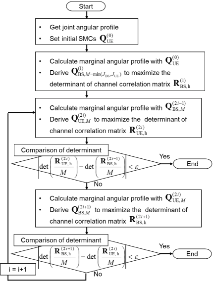
Figure 8: Calculation procedure of iterative optimization at BS and UE.

3.3 Rank adaptation

The rank of the channel correlation matrix depends on the numbers of BS and UE antennas or those of BS and UE spherical modes, and the initial condition defined by the angular profile. Thus, the optimal rank, i.e., the optimal number of streams, should be derived to maximize the average channel capacity. From the results of the analog beamforming weights’ selection or iterative calculation, the optimal number of streams can be obtained as follows.

$$M^{\mathrm{opt}} =\mathop{\rm arg~{}max}\limits_{M}\sum_{m=1}^{M}\bar{C}_{m}$$

$$=\mathop{\rm arg~{}max}\limits_{M}\sum_{m=1}^{M}\mathrm{E}\left[\log_{2}\left(1+\lambda_{m}\frac{P_{\mathrm{t}}}{MP_{\mathrm{n}}}\right)\right],$$ (30)

where $\lambda_{m}$ is an eigenvalue of the matrix $\mathbf{R}_{\mathrm{BS,h}}$.

3.4 Convergence of the objective function

The objective function to maximize the determinant of the channel correlation matrix converges because it is bounded above and monotonically increasing. Since the number of streams is limited, the determinant of the channel correlation matrix is bounded above by the product of a finite number of eigenvalues determined by the number of streams. Furthermore, when the duality of the channels is assumed, the channel correlation matrix of the $(2n+1)$-th calculation is expressed by using $\mathbf{Q}_{\mathrm{BS}}^{(2n+1)}$ and $\mathbf{R}_{\mathrm{BS,sph}}^{(2n+1)}$ and by using $\mathbf{Q}_{\mathrm{UE}}^{(2n)}$ and $\mathbf{R}_{\mathrm{UE,sph}}^{(2n+2)}$.

$$\mathbf{Q}_{\mathrm{BS}}^{(2n+1)\mathrm{T}}\mathbf{R}_{\mathrm{BS,sph}}^{(2n+1)}\mathbf{Q}_{\mathrm{BS}}^{(2n+1)\mathrm{*}} = \mathbf{Q}_{\mathrm{UE}}^{(2n)\mathrm{T}}\mathbf{R}_{\mathrm{UE,sph}}^{(2n+2)}\mathbf{Q}_{\mathrm{UE}}^{(2n)\mathrm{*}}$$ (31)

where superscripts indicate the iteration counts. By the $(2n+2)$-th calculation, the matrix of SMCs is derived and the determinant is the same or larger than that of the previous calculation. Thus, the determinant is monotonically increasing as follows.

$$\det\mathbf{Q}_{\mathrm{UE}}^{(2n)\mathrm{T}}\mathbf{R}_{\mathrm{UE,sph}}^{(2n+2)}\mathbf{Q}_{\mathrm{UE}}^{(2n)\mathrm{*}} \leq \prod_{m=1}^{M^{(2n+2)}}\lambda_{m}^{(2n+2)}$$

$$= \det\mathbf{U}^{(2n+2)\mathrm{H}}\mathbf{R}_{\mathrm{UE,sph}}^{(2n+2)}\mathbf{U}$$

$$= \det\mathbf{Q}_{\mathrm{UE}}^{(2n+2)\mathrm{T}}\mathbf{R}_{\mathrm{UE,sph}}^{(2n+2)}\mathbf{Q}_{\mathrm{UE}}^{(2n+2)\mathrm{*}},$$

where $\mathbf{U}^{(2n+2)}$ and $\lambda_{m}^{(2n+2)}$ are the eigenvectors’ matrix and the $m$-th eigenvalue of $\mathbf{R}_{\mathrm{UE,sph}}^{(2n+2)}$ respectively.

From the above, the objective function converges because it is bounded above and monotonically increasing. Additionally, the convergence may be slow when the channels between BS and UE are correlated as shown in Sect. 5.2 of [10]. In such a case, the calculation is finished based on the iteration counts, elapsed time, and so on.

3.5 Projection to conditional beam patterns

The method to derive the semi-optimal beam patterns at BS are introduced and the same way is used at UE. In general, the current distribution is derived by solving the following integral equation.

$$\mathbf{q}_{\mathrm{BS},m}^{\mathrm{opt}}\!=\!\int_{V_{\mathrm{BS}}}\!\!\vec{J}_{\mathrm{BS},m}(r_{\mathrm{BS}},\theta_{\mathrm{BS}},\phi_{\mathrm{BS}})\cdot\vec{\mathbf{f}}_{\mathrm{BS}}(r_{\mathrm{BS}},\theta_{\mathrm{BS}},\phi_{\mathrm{BS}})\mathrm{d}V_{\mathrm{BS}},$$ (33)

where $\mathbf{q}_{\mathrm{BS},m}^{\mathrm{opt}}\!\in\!\mathbb{C}^{J_{\mathrm{BS}}\times 1}$ is a vector of SMCs corresponding the $m$-th optimal beam pattern, $\vec{J}_{\mathrm{BS},m}(r_{\mathrm{BS}},\theta_{\mathrm{BS}},\phi_{\mathrm{BS}})$ is the $m$-th current distribution on the antenna surface with volume $V_{\mathrm{BS}}$ and $\vec{\mathbf{f}}_{\mathrm{BS}}(r,\theta,\phi)\!\in\!\mathbb{C}^{J_{\mathrm{BS}}\times 1}$ is a vector of spherical wave functions representing radial standing waves at a location $(r,\theta,\phi)$. By using Galerkin method, which is one of the methods for solving the integral equation, Eq. (33) is represented as a linear equation as shown in [10], given by

$$\mathbf{q}_{\mathrm{BS},m}^{\mathrm{opt}}=\mathbf{Z}_{\mathrm{BS}}\mathbf{a}_{\mathrm{BS},m},$$ (34)

where $\mathbf{Z}_{\mathrm{BS}}\!\in\!\mathbb{C}^{J_{\mathrm{BS}}\times L}$ is a transformation matrix from the space of antenna surface to the far field and $\mathbf{a}_{\mathrm{BS},m}\!\in\!\mathbb{C}^{L\times 1}$ is a vector of the $m$-th current distribution coefficients. By using a Moore-Penrose inverse matrix $\mathbf{Z}_{\mathrm{BS}}^{+}\!\in\!\mathbb{C}^{L\times J_{\mathrm{BS}}}$, the current distribution coefficients are derived as the least squares and minimum norm solution.

$$\mathbf{a}_{\mathrm{BS},m}=\mathbf{Z}_{\mathrm{BS}}^{+}\mathbf{q}_{\mathrm{BS},m}^{\mathrm{opt}}.$$ (35)

The SMCs’ vector of the semi-optimal beam pattern radiated from the antenna surface is expressed as follows.

$$\mathbf{q}_{\mathrm{BS},m}^{\mathrm{semi}}=\mathbf{Z}_{\mathrm{BS}}\mathbf{a}_{\mathrm{BS},m}=\mathbf{Z}_{\mathrm{BS}}\mathbf{Z}^{+}\mathbf{q}_{\mathrm{BS},m}^{\mathrm{opt}}.$$ (36)

$\mathbf{Z}_{\mathrm{BS}}\mathbf{Z}_{\mathrm{BS}}^{+}$ is an orthogonal projection operator [18], thus the SMCs’ vector of the optimal beam pattern is projected to that of the conditional beam pattern and the semi-optimal beam pattern is obtained as corresponding to the current distribution of the least squares and the minimum norm solution among the conditional beam patterns that can be radiated from the antenna surface.

Table 2 shows examples of the assumed antenna surface for the BS antenna defined by a radius of the spherical surface $R$ and a range of angle $\theta_{\mathrm{c}},\phi_{\mathrm{c}}$. Three cases of surfaces are considered such as Plane, 1/32-sphere and Hemisphere. They are included in the sphere with the radius $r_{0,\mathrm{BS}}$, which is the same volume as the 2-dimensional square array antennas in the cases of full-array and sub-array. Examples of configurations and current distributions are shown in Fig. 9 by using the conventional planar patch array and the hemisphere antenna surface that we proposed.

Table 2: Examples of antenna surfaces.

	Plane	1/32-sphere	Hemisphere
$R$	–	$\max\{r_{0}/(\sqrt{2}\sin\theta_{c}),r_{0}/(\sqrt{2}\sin\phi_{c})\}$	$r_{0}$
($\theta_{\mathrm{c}}$, $\phi_{\mathrm{c}}$)	–	($\pi/8$, $\pi/8$)	($\pi/2$, $\pi/2$)

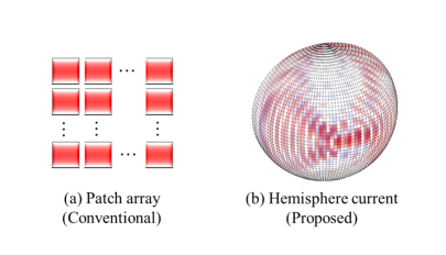
Figure 9: Examples of current distributions of conventional array and proposed current surface.

4 Numerical analysis

In this section, the beam patterns by using OBPB and conventional hybrid beamforming are derived and discussed.

4.1 Analysis condition

Conditions of analysis are shown in Table 3 and the angular profile is defined by using a multivariate Gaussian distribution as shown in Figs. 11, 11 and Table 4 with only $\theta$ polarization component. In the analysis, the $\phi$-plane and $\theta$-plane indicate the $xy$-plane and $xz$-plane as shown in Fig. 6 respectively. $\lambda_{0}$ is a wavelength, $\mathbf{P}$ is a correlation matrix between each variates, the standard deviations of $\theta$ components are $\sigma_{\mathrm{BS},\theta},\sigma_{\mathrm{UE},\theta}$, and the standard deviations of $\phi$ components are $\sigma_{\mathrm{BS},\phi},\sigma_{\mathrm{UE},\phi}$. The mean and correlation matrix between variables are defined as 3GPP UMa NLOS model at 30 GHz [21].

In the conventional hybrid beamforming case, the 2-dimensional square array antennas are used and each element has a beam pattern defined in [21]. To compare the characteristics of the proposed and conventional hybrid beamforming in the same antenna volume, the antenna area of the patch array at the UE side is a square having sides with a fixed length $A_{\mathrm{UE}}$ and the elements are allowed to be overlapped when the number of UE antennas becomes large. In the case of sub-array configuration, the number of antenna elements in the sub-array is chosen from 10 types of sub-array configurations to maximize the average channel capacity, such as ($N_{\mathrm{BS,sub,V}}\times N_{\mathrm{BS,sub,H}}$) = ($1\times 4$), ($2\times 2$), ($4\times 1$), ($1\times 8$), ($2\times 4$), ($4\times 2$), ($8\times 1$), ($2\times 8$), ($4\times 4$), ($8\times 2$).

The current surfaces of the proposed cases are shown in Table 2. They are defined as the same antenna volume as the conventional array configurations, which are defined by the same radii of BS and UE antenna volume $r_{\mathrm{0,BS}},r_{\mathrm{0,UE}}$. The relationship between the proposed and the conventional antenna configurations is shown in Fig. 12, where they face each other with a direction of $(\mu_{\mathrm{BS},\theta},\mu_{\mathrm{BS},\phi})=(90\ \mathrm{[deg.]},0\ \mathrm{[deg.]})$ at BS and that of $(\mu_{\mathrm{UE},\theta},\mu_{\mathrm{UE},\phi})=(90\ \mathrm{[deg.]},0\ \mathrm{[deg.]})$ at UE.

Table 3: Analysis condition.

	$N_{\mathrm{BS}}=64$
Number of antennas	$N_{\mathrm{UE}}=4,9,16,25,36,49$
	$N_{\mathrm{BS,sub}}=4,8,16$
Spacing of BS antenna elements	$\frac{\lambda_{0}}{2}$
Spacing of UE antenna elements	$\frac{1}{\sqrt{N_{\mathrm{UE}}}-1}\cdot\frac{\lambda_{0}}{2}$
Antenna size	$\frac{\lambda_{0}}{2}$
Beam interval coefficient	$a$ = 4
Radius of antenna volume	$r_{\mathrm{0,BS}}=\left(\frac{7\lambda_{0}}{2}+\frac{\lambda_{0}}{2}\right)/\sqrt{2}$
	$r_{\mathrm{0,UE}}=\left(\frac{\lambda_{0}}{2}+\frac{\lambda_{0}}{2}\right)/\sqrt{2}$
Number of spherical modes	$J_{\mathrm{BS}}=646$
	$J_{\mathrm{UE}}=48$
Initial beam pattern	omni-directional pattern
for iterative optimization
Initial number of streams	1
for iterative optimization
Received SNR with	-12 dB
omni directivities in SISO
Basis function	Dirac delta function
	1% of the difference
Allowable difference	between the last value and
	the previous value

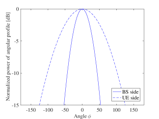
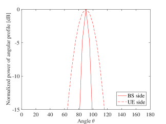
Figure 10: Angular profile in $\phi$-plane.

Figure 11: Angular profile in $\theta$-plane.

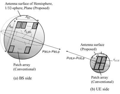
Figure 12: Antenna configurations for proposed and conventional methods.

Table 4: Parameters of angular profile.

	$\mu_{\mathrm{BS},\theta}=$ 90 [deg.]
Angle of departure	$\mu_{\mathrm{BS},\phi}=$ 0 [deg.]
and arrival	$\mu_{\mathrm{UE},\theta}=$ 90 [deg.]
	$\mu_{\mathrm{UE},\phi}=$ 0 [deg.]
	$\sigma_{\mathrm{BS},\theta}=$ 4 [deg.]
Angular spread of	$\sigma_{\mathrm{BS},\phi}=$ 21 [deg.]
departure and arrival	$\sigma_{\mathrm{UE},\theta}=$ 11 [deg.]
	$\sigma_{\mathrm{UE},\phi}=$ 48 [deg.]
Covariance matrix $\mathbf{P}$	$\left[\begin{array}[]{cccc}1&0.3&0&0.2\\ 0.3&1&0.1&0.4\\ 0&0.1&1&0\\ 0.2&0.4&0&1\\ \end{array}\right]$
Polarization	Only $\theta$ polarization

4.2 Beam patterns

The beam patterns of the full-array configuration (Full-array) are derived as shown in Figs. 16, 16, 16 and 16 in the case of $N_{\mathrm{UE}}=4$. By using the received power of each stream for the weight selection, the patterns near the peak of the angular profile are chosen. It causes the degradation of the average channel capacity due to the high correlation between the beam patterns. On the other hand, by using the determinant of the channel correlation matrix, the average channel capacity does not degrade compared with the previous case because sufficiently separated and low correlated patterns are selected by considering the determinant. However, as the number of streams increases, the peaks of the selected patterns are away from the peaks of the given angular profile. Thus, it causes the loss of the received power and the capacity degradation.

Next, the optimal beam patterns of the sub-array configuration (Sub-array) is shown in Figs. 20 and 20 in the case of $N_{\mathrm{UE}}=4$. The same beam patterns are selected in all groups of sub-arrays by using either the received power and the determinant. The number of antenna elements of the sub-array group is derived as ($N_{\mathrm{BS,sub,V}}\times N_{\mathrm{BS,sub,H}}$)= ($8\times 2$) in the case of $N_{\mathrm{UE}}=4$, ($N_{\mathrm{BS,sub,V}}\times N_{\mathrm{BS,sub,H}}$)= ($4\times 2$) in the case of $N_{\mathrm{UE}}=9$, and ($N_{\mathrm{BS,sub,V}}\times N_{\mathrm{BS,sub,H}}$)= ($4\times 1$) in the other cases. The angular profile in $\theta$-plane is narrower than that of $\phi$-plane in the analysis. Thus, the beam patterns in $\theta$-plane should be narrow as well and the sub-array is better to be a vertical array than a horizontal array. Furthermore, it is found that the same beam patterns are chosen in this case. From the results, the beam patterns are sufficiently decorrelated even though using the same analog beamforming weight vector because the effective radio wave sources are separated from with each other.

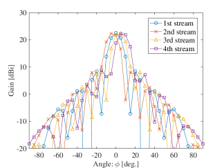
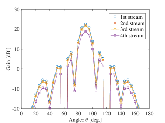
Figure 13: Beam patterns of Full-array in $\phi$-plane derived by Received power ($N_{\mathrm{UE}}=4$).

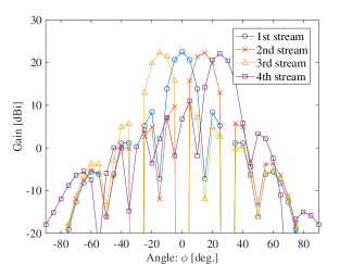
Figure 14: Beam patterns of Full-array in $\theta$-plane derived by Received power ($N_{\mathrm{UE}}=4$).

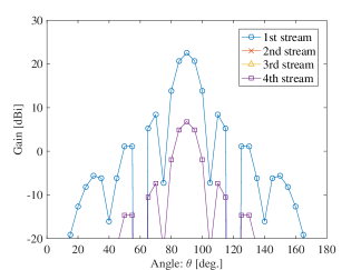
Figure 15: Beam patterns of Full-array in $\phi$-plane derived by Determinant ($N_{\mathrm{UE}}=4$).

Figure 16: Beam patterns of Full-array in $\theta$-plane derived by Determinant ($N_{\mathrm{UE}}=4$).

By using OBPB on the spherical surface, the optimal beam patterns are derived as shown in Fig. 20 to Fig. 24. It is found that the pattern of the 1st stream has its peak and the other patterns have null towards the peak of the angular profile. In the case of Plane, the gains degrade because the planar antenna surface cannot make some beam patterns due to constraints of the conditional current distributions on the surface. When the current surface becomes curved from Plane to 1/32-sphere and Hemisphere, the power of the beam pattern is directed to the peak of the angular profile. Thus, the loss of the transmission power becomes small while having low correlation and the average channel capacity can be improved. As the current surface is curved as 1/32-sphere and Hemisphere, the complexity of the derived beam patterns becomes high and they have low gains of side lobes compared to Plane because the various directions of currents are achieved.

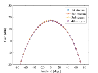
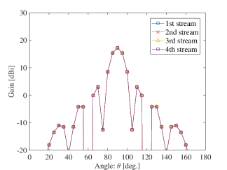
Figure 17: Beam patterns of Sub-array in $\phi$-plane ($N_{\mathrm{UE}}=4$).

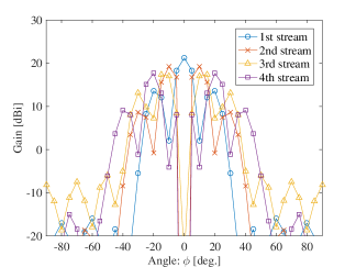
Figure 18: Beam patterns of Sub-array in $\theta$-plane ($N_{\mathrm{UE}}=4$).

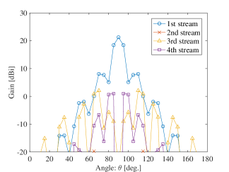
Figure 19: Semi-optimal beam patterns of Plane in $\phi$-plane.

Figure 20: Semi-optimal beam patterns of Plane in $\theta$-plane.

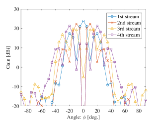
Figure 21: Semi-optimal beam patterns of 1/32-sphere in $\phi$-plane.

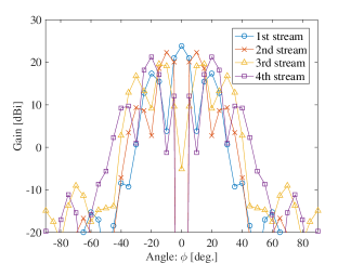
Figure 22: Semi-optimal beam patterns of 1/32-sphere in $\theta$-plane.

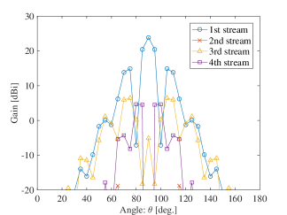
Figure 23: Semi-optimal beam patterns of Hemisphere in $\phi$-plane.

Figure 24: Semi-optimal beam patterns of Hemisphere in $\theta$-plane.

To compare the proposed semi-optimal patterns to the conventional beam patterns, three cases of 3-D beam patterns are shown in Figs. 25 - 27. In the case of the conventional beam selection, one main lobe is mainly used as shown in Fig. 25. On the other hand, in the case of the beams of Plane (Fig. 26) and Hemisphere (Fig. 27), it is found that there are multiple narrow beams in the range of the angular profile for all streams. It means that both the main and side lobes are useful by using OBPB method and the received power becomes large in each stream. Thus, the channel capacity is improved.

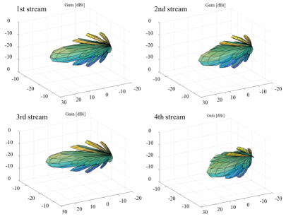
Figure 25: 3-D beam patterns of Full-array derived by Determinant ($N_{\mathrm{UE}}=4$).

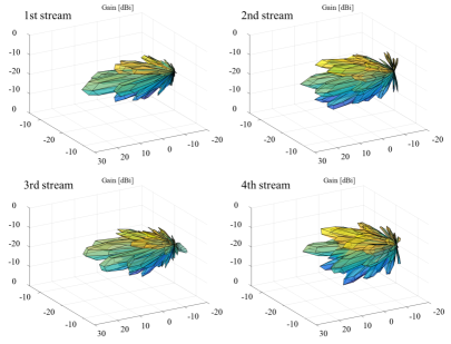
Figure 26: 3-D semi-optimal beam patterns of Plane.

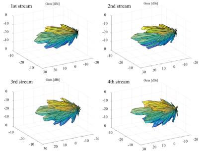
Figure 27: 3-D semi-optimal beam patterns of Hemisphere.

4.3 Channel correlation matrix with optimal beam patterns

The normalized channel correlation matrix is derived which components are derived as

$$|\tilde{r}_{i,j}|=\frac{|r_{i,j}|^{2}}{\sqrt{|r_{i,i}||r_{j,j}|}},$$ (37)

where $r_{i,j}$ is the $i$-th row and $j$-th column component of the channel correlation matrix $\mathbf{R}_{\mathrm{BS,h}}$ containing the derived beam patterns. The components and determinant of the channel correlation matrix in the case of $N_{\mathrm{UE}}=4$ are shown in Table 5.

In the case of Hemisphere, the same number of streams and channel capacity with the optimal beam patterns are achieved. It is also found that the channel correlation matrix is completely orthogonalized and the determinant is larger than that of the other methods. In the cases of 1/32 sphere and Plane, the channel correlation matrices are almost orthogonalized and their determinants are much larger than that of the conventional hybrid beamforming. From the results, it is found that using the beam patterns derived by OBPB improves the SU-MIMO system performance.

In the case of Full-array, the determinant of the channel correlation matrix by the beam selection using the determinant is larger than that using the received power because of low correlation. Therefore, the average channel capacity is slightly improved. In the case of Sub-array, the correlation coefficients between streams are lower than those of Full-array using the received power because the effective sources of the beam patterns are separated from each other in Sub-array. It is found that Sub-array is preferable to Full-array using the beam selection in terms of the received power when the correlation between selected beam patterns are high.

Table 5: Normalized channel correlation matrix from 1st to 4th streams ($N_{\mathrm{UE}}=4$).

Method	Normalized channel correlation matrix	Determinant [dB]
Hemisphere	$\left[\begin{array}[]{cccc}1&0&0&0\\ 0&1&0&0\\ 0&0&1&0\\ 0&0&0&1\\ \end{array}\right]$	168
1/32-sphere	$\left[\begin{array}[]{cccc}1&0.00010&0.00052&0.00033\\ 0.00010&1&0.00028&0.00066\\ 0.00052&0.00028&1&0.00084\\ 0.00033&0.00066&0.00084&1\\ \end{array}\right]$	168
Plane	$\left[\begin{array}[]{cccc}1&0&0.014&0\\ 0&1&0&0.021\\ 0.014&0&1&0\\ 0&0.021&0&1\\ \end{array}\right]$	144
Full-array (Received power)	$\left[\begin{array}[]{cccc}1&0.92&0.92&0.71\\ 0.92&1&0.71&0.41\\ 0.92&0.71&1&0.92\\ 0.71&0.41&0.92&1\\ \end{array}\right]$	55.5
Full-array (Determinant)	$\left[\begin{array}[]{cccc}1&0.10&0.10&0.23\\ 0.10&1&0.13&0.34\\ 0.10&0.13&1&0.21\\ 0.23&0.34&0.21&1\\ \end{array}\right]$	102
Sub-array	$\left[\begin{array}[]{cccc}1&0.31&0.0025&0\\ 0.31&1&0.31&0.0025\\ 0.0025&0.31&1&0.31\\ 0&0.0025&0.31&1\\ \end{array}\right]$	102

4.4 Optimal number of streams and average channel capacity

The optimal number of streams and the average channel capacity, corresponding to the number of conventional UE antennas in the given sphere, are depicted in Figs. 28 and 29. When the number of conventional UE antennas becomes large in Full-array, the optimal number of streams increases to 20 and 27 by using Received power and Determinant respectively. In Sub-array, the maximum value of the number of streams is limited to $N_{\mathrm{BS}}/N_{\mathrm{BS,sub}}$ which is up to 16 in the analysis. It is found that the average channel capacity also increases and Sub-array is more effective than Full-array using Power when there is sufficient orthogonality of streams.

In the case of Proposed, the optimal number of streams and the average channel capacity do not vary since the radii of antenna volume at both BS and UE sides are constant. Both the number of streams and the average channel capacity increase by using the optimal patterns derived using OBPB because the patterns are more matched to the angular profile than those of Full-array and Sub-array. The average channel capacity becomes 3.5 times or larger than using Full-array and Sub-array in the cases of 1/32-sphere and Hemisphere. It is because the patterns match the angular profile and low correlated by their orthogonality.

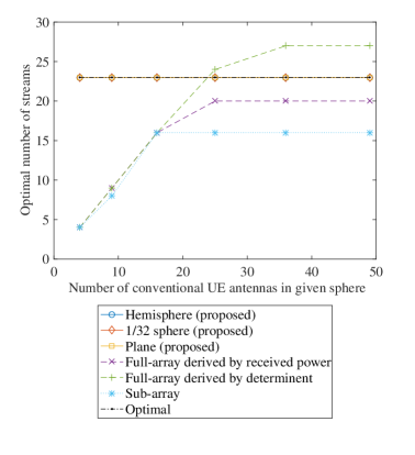
Figure 28: Optimal number of streams.

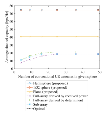
Figure 29: Average channel capacity.

5 Conclusion

In this paper, we proposed a method that can derive optimal beam patterns of analog beamforming for SU massive MIMO by iterative optimization. We also derived the semi-optimal beam patterns on the assumed antenna surface, such as Plane, 1/32-sphere and Hemisphere, by using OBPB. Numerical analyses showed that the proposal could achieve the same number of streams and channel capacity as offered by optimal beam patterns for the case of a hemispherical surface. Also, it is clarified that the average channel capacity is 3.5 times or larger by using the semi-optimal beam patterns derived by OBPB than that by using the conventional hybrid beamforming. The semi-optimal beam patterns yield orthogonal streams because the patterns are matched to the angular profile and low correlated with each other. Therefore, the analog beamforming by OBPB is more effective for SU-massive MIMO than the conventional analog beamforming as it offers higher average channel capacity.

Maki Arai received the B.E. and M.E. degrees in electrical and electronic engineering from the Tokyo Institute of Technology, in 2010 and 2012. She joined the NTT Network Innovation Laboratories, Nippon Telegraph and Telephone Corporation (NTT) in 2012. From 2015, she is a doctor course student at Tokyo Institute of Technology. Her current research interests are high speed wireless communication systems and analysis and design of MIMO antennas. She received the Research Encouragement Award of the Institute of Electrical Engineers of Japan (IEEJ) in 2010, the Antenna and Propagation Research Commission Student Award from the Institute of Electronics, Information and Communication Engineers (IEICE) in 2012, and the Young Engineers Award from the IEICE in 2015.

Kei Sakaguchireceived the B.E. degree in electrical and computer engineering from Nagoya Institute of Technology, Japan in 1996, and the M.E. degree in information processing from Tokyo Institute of Technology, Japan in 1998, and the Ph.D. degree in electrical and electronic engineering from Tokyo Institute of technology in 2006. Currently, he is a Professor at Tokyo Institute of Technology in Japan and at the same time he is working at Fraunhofer HHI in Germany as a Senior Scientist. He received the Outstanding Paper Awards from SDR Forum and IEICE in 2004 and 2005, respectively, the Tutorial Paper Award from IEICE Communication Society in 2006, and the Bast Paper Awards from IEICE Communication Society in 2012, 2013, and 2015. He is currently playing a role of the Industry Panel co-chair in IEEE Globecom 2017. His current research interests are 5G cellular networks, sensor networks, and wireless energy transmission. He is a member of IEEE.

Kiyomichi Arakireceived the Ph.D. degree from Tokyo Institute of Technology, Japan, in 1978. In In 1979-1980 and 1993-1994, he was a visiting research scholar at University of Texas, Austin and University of Illinois, Urbana, respectively. Since 1995 to 2014 he has been a Professor at Tokyo Institute of Technology, and now an Emeritus Professor. He has numerous journals and peer review publications in RF ferrite devices, RF circuit theory, electromagnetic field analysis, software defined radio, array signal processing, UWB technologies, wireless channel modeling, MIMO communication theory, digital RF circuit design, information security, and coding theory.

References

- [1] L. Lu, G. Y. Li, A. L. Swindlehurst, A. Ashikhmin, R. Zhang, “An Overview of Massive MIMO: Benefits and Challenges,” IEEE Journal of Selected Topics in Signal Processing, vol. 8, no. 5, pp. 742-758, Oct. 2014.
- [2] H. Ji et al., “Overview of Full-Dimension MIMO in LTE-Advanced Pro,” IEEE Communications Magazine, vol. 55, no. 2, pp. 176-184, February 2017.
- [3] Y. H. Nam et al., “Full-dimension MIMO (FD-MIMO) for next generation cellular technology,” IEEE Communications Magazine, vol. 51, no. 6, pp. 172-179, June 2013.
- [4] F. Sohrabi, W. Yu, “Hybrid Analog and Digital Beamforming for mmWave OFDM Large-Scale Antenna Arrays,” IEEE Journal on Selected Areas in Communications, vol. 35, no. 7, pp. 1432-1443, July 2017.
- [5] Z. Xiao, P. Xia, X. G. Xia, “Channel Estimation and Hybrid Precoding for Millimeter-Wave MIMO Systems: A Low-Complexity Overall Solution,” IEEE Access, vol. 5, pp. 16100-16110, 2017.
- [6] J. Nsenga, A. Bourdoux and F. Horlin, “Mixed Analog/Digital Beamforming for 60 GHz MIMO Frequency Selective Channels,” 2010 IEEE International Conference on Communications, Cape Town, 2010, pp. 1-6.
- [7] T. Obara, S. Suyama, J. Shen, Y. Okumura, “Joint Processing of Analog Fixed Beamforming and CSI-Based Precoding for Super High Bit Rate Massive MIMO Transmission Using Higher Frequency Bands,” IEICE Trans. on Commun., vol.E98-B, no. 8, pp. 1474-1481, 2015.
- [8] B. L. Ng et al., “Fulfilling the promise of massive MIMO with 2D active antenna array,” 2012 IEEE Globecom Workshops, Anaheim, CA, 2012, pp. 691-696.
- [9] A. L. Swindlehurst, E. Ayanoglu, P. Heydari, F. Capolino, “Millimeter-wave massive MIMO: the next wireless revolution?,” IEEE Communications Magazine, vol. 52, no. 9, pp. 56-62, September 2014.
- [10] M. Arai, M. Iwabuchi, K. Sakaguchi, K. Araki, “Optimal Design Method of MIMO Antenna Directivities and Corresponding Current Distributions by Using Spherical Mode Expansion,” IEICE Trans. on Commun. E100.B(10), 1891-1903, 2017.
- [11] J. E. Hansen, “Spherical near-field antenna measurements theory and practice,” Peter Peregrinus Ltd. IEEE electromagnetic waves series 26, 1988.
- [12] A. A. Glazunov, M. Gustafsson, A. F.Molisch, F. Tufvesson, and G. Kristensson, “Spherical Vector Wave Expansion of Gaussian Electromagnetic Fields for Antenna-Channel Interaction Analysis,” IEEE Trans. on Antennas and Propagation, vol.57, no.7, July 2009.
- [13] Y. Miao, K. Haneda, M. Kim and J. Takada, “Antenna De-Embedding of Radio Propagation Channel With Truncated Modes in the Spherical Vector Wave Domain,” IEEE Trans. on Antennas and Propagation, vol. 63, no. 9, pp. 4100-4110, Sept. 2015.
- [14] J. Driscoll, and D. Healy, Jr, “Computing Fourier transforms and convolutions on the 2-sphere,” J. Advanced in Applied Mathematics, vol.15, pp. 202-250, 1994.
- [15] E. W. Weisstein, “Spherical Harmonic,” MathWorld–A Wolfram Web Resource. http://mathworld.wolfram.com/SphericalHarmonic.html.
- [16] Q. T. Zhang, X.W. Cui, and X.M. Li, “Very tight capacity bounds for MIMO-correlated Rayleigh-fading channels,” IEEE Trans. Wireless Commun., vol.4, no.2, pp.681-688, Mar. 2005.
- [17] E. F. Beckenbach, R. Bellman, “Inequalities,” Springer. p. 64, 1965.
- [18] O. M. Baksalary, G. Trenkler, “Functions of orthogonal projectors involving the Moore-Penrose inverse,” Computers & Mathematics with Applications, Volume 59, Issue 2, pp 764-778, 2010.
- [19] K. V. Mardia, P. E. Jupp, “Directional Statistics,” Springer Texts in Statistics, Chapter 5, pp. , 2009.
- [20] M. Bilodeau, D. Brenner, “Theory of multivariate statistics,” Wiley Series in Probability and Statistics, Chapter 3, pp. 58-59, 1999.
- [21] 3GPP TR 38.900, “3rd Generation Partnership Project; Technical Specification Group Radio Access Network; Study on channel model for frequency spectrum above 6 GHz (Release 14),” V14.3.1, 2017-07-03.