Hamiltonian hydrodynamics of eccentric discs

Abstract

We show that the ideal hydrodynamics of an eccentric astrophysical disc can be derived from a variational principle. The nonlinear secular theory describes the slow evolution of a continuous set of nested elliptical orbits as a result of the pressure in a thin disc. In the artificial but widely considered case of a 2D disc, the hydrodynamic Hamiltonian is just the orbit-averaged internal energy of the disc, which can be determined from its eccentricity distribution using the geometry of the elliptical orbits. In the realistic case of a 3D disc, the Hamiltonian needs to be modified to take into account the dynamical vertical structure of the disc. The simplest solutions of the theory are uniformly precessing nonlinear eccentric modes, which make the energy stationary subject to the angular momentum being fixed. We present numerical examples of nonlinear eccentric modes up to their limiting amplitudes. Although it lacks dissipation, which is important in many astrophysical contexts, this formalism allows a simpler theoretical approach to the nonlinear dynamics of eccentric discs than that derived from stress integrals, and also connects better with established methods of celestial mechanics for cases in which the disc interacts gravitationally with one or more orbital companion.

1 Introduction

Eccentric gaseous discs, in which the dominant motion of the fluid consists of elliptical Keplerian orbits around a central mass, have numerous applications in astrophysics. Circumbinary discs around binary black holes in galactic nuclei, or around young binary stars in protoplanetary environments, have been found in several numerical simulations to become eccentric, even if the binary orbit is circular (MacFadyen & Milosavljević, 2008; Miranda, Muñoz & Lai, 2017; Thun, Kley & Picogna, 2017). Eccentricity leads to modulation of the accretion rate and affects the properties of the disc as well as the evolution of the binary (Artymowicz & Lubow, 1996). Similar physics allows the growth of eccentricity of planets orbiting in gaps or cavities in protoplanetary discs (Papaloizou, Nelson & Masset, 2001; Goldreich & Sari, 2003; Kley & Dirksen, 2006; D’Angelo, Lubow & Bate, 2006; Rice, Armitage & Hogg, 2008; Duffell & Chiang, 2015; Teyssandier & Ogilvie, 2016, 2017; Rosotti et al., 2017; Ragusa et al., 2018). The mechanism is related to those already investigated for circumstellar discs in ‘superhump’ binary stars (Whitehurst, 1988; Lubow, 1991a, b; Smith et al., 2007; Kley, Papaloizou & Ogilvie, 2008) and for planetary rings (Goldreich & Tremaine, 1981; Borderies, Goldreich & Tremaine, 1983). Circumstellar discs with companions on sufficiently inclined orbits can undergo Kozai–Lidov cycles in which the disc becomes highly eccentric (Martin et al., 2014; Fu, Lubow & Martin, 2015a, b; Zanazzi & Lai, 2017; Lubow & Ogilvie, 2017). Eccentric discs are also increasingly discussed in connection with tidal disruption events in which a star on a nearly parabolic orbit passes too close to the black hole at the centre of a galaxy (e.g. Guillochon, Manukian & Ramirez-Ruiz, 2014; Bonnerot et al., 2016; Cao et al., 2018), or a planetesimal is disrupted around a white dwarf (Manser et al., 2016; Cauley et al., 2018; Miranda & Rafikov, 2018).

In many of these applications the eccentricities and their gradients are not small enough to be well described by the linear theories discussed by Papaloizou (2002), Goodchild & Ogilvie (2006), Ogilvie (2008) and Teyssandier & Ogilvie (2016). A nonlinear theory of eccentric discs was developed by Ogilvie (2001) and rederived from an alternative viewpoint by Ogilvie & Barker (2014). Evolutionary equations in one spatial dimension were obtained for the shape and mass distribution of the disc; however, these equations are complicated because they contain nonlinear functions of the eccentricity, eccentricity gradient and twist that must be (pre-)computed numerically by solving a set of nonlinear ordinary differential equations around each orbit and evaluating a number of integrals of stress components combined with geometrical factors. Perhaps as a result of this complexity, the nonlinear aspects of the theory have not been investigated widely in the literature, although inviscid nonlinear modes have been computed and tested in 2D simulations by Barker & Ogilvie (2016).

The purpose of this paper is to present an alternative, and in some ways much simpler, approach to the nonlinear dynamics of eccentric discs. We focus on the special case in which dissipation can be neglected; it is then possible to apply a Hamiltonian formulation, which has attractive mathematical properties and assists in the physical interpretation of the solutions. As in the case of the classical dynamics of systems of particles or rigid bodies, Hamiltonian methods are useful mainly because they clarify the mathematical structure of the problem and provide new insights.

It is well known from the linear theory that eccentricity propagates through gaseous discs predominantly by means of pressure, in the form of a dispersive wave. Viscous forces or other dissipative effects generally contribute a slow diffusion and/or damping of eccentricity. The ideal fluid theories that we discuss in this paper describe the nonlinear version of the propagation of eccentricity by means of pressure, and neglect the weaker effects of viscous forces and other dissipative effects. Self-gravity can also make an important contribution to the propagation of eccentricity, e.g. in planetary rings; it is relatively easy to include within the Hamiltonian framework but we do not consider it in this paper.

This paper is structured as follows. We first discuss the geometry of eccentric discs (Section 2) by defining a set of canonical variables and analysing the related orbital coordinate system. We then derive the evolutionary equations for an eccentric disc from a Hamiltonian (Section 3) and point out some of their mathematical properties. The known linear theory is verified in Section 4. Section 5 discusses special modal solutions of the nonlinear equations and gives numerical examples. Conclusions are given in Section 6 and some mathematical derivations appear in the appendices.

2 Geometry of eccentric discs

Let $(x,y)$ and $(r,\phi)$ be Cartesian and polar coordinates in a plane, related by

$$x=r\cos\phi,\qquad y=r\sin\phi.$$ (1)

The polar equation for an elliptical Keplerian orbit of semimajor axis $a$, eccentricity $e$ and longitude of periapsis $\varpi$ (‘curly pi’) is

$$r=\frac{a(1-e^{2})}{1+e\cos f},$$ (2)

where

$$f=\phi-\varpi$$ (3)

is the true anomaly. Equivalently,

$$r=a(1-e\cos E),$$ (4)

where $E$ is the eccentric anomaly, which satisfies

$$\cos f=\frac{\cos E-e}{1-e\cos E},\qquad\sin f=\frac{\sqrt{1-e^{2}}\sin E}{1-e\cos E}$$ (5)

as well as Kepler’s equation

$$M=E-e\sin E,$$ (6)

where (in this Section only) $M=n(t-\tau)$ is the mean anomaly, $n=(GM_{1}/a^{3})^{1/2}$ is the mean motion, $M_{1}$ is the central mass and $\tau$ is the time of periapsis passage.

For some purposes, such as bringing out the Hamiltonian structure of the dynamics, it is convenient to use canonical variables such as the modified Delaunay variables

$$\Lambda=\sqrt{GM_{1}a},\qquad\lambda=M+\varpi,$$ (7)

$$\Gamma=\Lambda\left(1-\sqrt{1-e^{2}}\right),\qquad\gamma=-\varpi.$$ (8)

These are action–angle variables, with one pair $(\Lambda,\lambda)$ describing the orbital motion and the other pair $(\Gamma,\gamma)$ describing the eccentricity. More specifically, $\Lambda$ identifies the orbit and determines its period and energy, while $\lambda$ (the mean longitude) is an orbital phase that increases linearly in time by $2\pi$ per orbital period. Then $\Gamma$ is a positive-definite measure of the eccentricity of the orbit, being proportional to $e^{2}$ when $e^{2}\ll 1$, while $\gamma$ determines the orientation of the ellipse.

A planar eccentric disc involves a continuous set of nested elliptical orbits. We can describe the shape of the disc by considering $e$ and $\varpi$ to be functions of $a$. The derivatives of these functions are written as $e_{a}=\mathrm{d}e/\mathrm{d}a$ and $\varpi_{a}=\mathrm{d}\varpi/\mathrm{d}a$. Equivalently, when using modified Delaunay variables, we can consider $\Gamma$ and $\gamma$ to be functions of $\Lambda$, with derivatives $\Gamma_{\Lambda}=\mathrm{d}\Gamma/\mathrm{d}\Lambda$ and $\gamma_{\Lambda}=\mathrm{d}\gamma/\mathrm{d}\Lambda$. Thus $e_{a}$ (or $\Gamma_{\Lambda}-\Gamma/\Lambda$) is a measure of the eccentricity gradient, while $\varpi_{a}$ (or $\gamma_{\Lambda}$) is a measure of the twist.

We can use $(\Lambda,\lambda)$ as a canonical orbital coordinate system covering the disc. The first coordinate $\Lambda$ labels the elliptical orbits, while around each orbit $\lambda$ ranges from $0$ to $2\pi$. The Cartesian coordinates $(x,y)$ can be deduced from $(\Lambda,\lambda)$ as follows. The value of $\Lambda$ determines $a$ and hence $e$ and $\varpi$ through the functions $e(a)$ and $\varpi(a)$. The value of $\lambda$ determines the mean anomaly $M=\lambda-\varpi$. Kepler’s equation can be solved to find the eccentric anomaly $E$. We can then find $f$ from equations (5). Thus we obtain $(r,\phi)$ and $(x,y)$.

In previous work (Ogilvie, 2001; Ogilvie & Barker, 2014) we have instead used $(\lambda,\phi)$ as an orbital coordinate system, where (in this paragraph only) $\lambda=a(1-e^{2})$ is the semilatus rectum. The geometry of eccentric discs is slightly easier to analyse when $e$ and $\varpi$ are considered to be functions of $\lambda$ rather than $a$. Also $\lambda$ is directly related to the orbital angular momentum, which is often more important than the orbital energy in the context of accretion discs. However, for the non-dissipative discs described by Hamiltonian hydrodynamics, it is more convenient to label the orbits using $a$, which is directly related to the orbital period and energy, and is a material invariant in the Hamiltonian theory. This approach also works better when combined with secular gravitational interactions, which similarly leave $a$ invariant.

By differentiating the above relations, we find that the Jacobian of the canonical orbital coordinate system $(\Lambda,\lambda)$ is

$$J=\frac{\partial(x,y)}{\partial(\Lambda,\lambda)}=J^{\circ}(a)j(E),$$ (9)

where

$$J^{\circ}=\frac{2}{n}$$ (10)

is the Jacobian for a circular disc and

$$j =1-\frac{\Gamma}{2\Lambda}-\frac{\Gamma_{\Lambda}}{2}+\frac{(\Gamma-\Lambda\Gamma_{\Lambda})\cos E}{2\sqrt{\Gamma(2\Lambda-\Gamma)}}$$

$$\qquad+\frac{\sqrt{\Gamma(2\Lambda-\Gamma)}\gamma_{\Lambda}\sin E}{2}$$

$$=\frac{1-e(e+ae_{a})}{\sqrt{1-e^{2}}}-\frac{ae_{a}\cos E}{\sqrt{1-e^{2}}}-ae\varpi_{a}\sin E$$ (11)

is dimensionless and purely related to the elliptical geometry of the disc. It can be verified that $J$ remains positive throughout the orbit provided that $(e+ae_{a})^{2}+(ae\varpi_{a})^{2}<1$. This condition was given by Statler (2001) and is exactly equivalent to the criterion $(e-\lambda e_{\lambda})^{2}+(\lambda e\varpi_{\lambda})^{2}<1$ given by Ogilvie (2001) in terms of the semilatus rectum. It is the condition for the eccentricity, eccentricity gradient and twist to be sufficiently small that neighbouring orbits do not intersect. Of course $e^{2}<1$ is also required for the orbits to be closed.

In the special case of an untwisted eccentric disc, for which $\varpi_{a}=0$, the condition for marginal orbital intersection, $e+ae_{a}=\pm 1$, is equivalent to

$$\frac{\mathrm{d}}{\mathrm{d}a}(a\mp ae)=0,$$ (12)

i.e. vanishing derivative of either periapsis or apoapsis distance with $a$. The orbits intersect when either the periapsis or apoapsis distance decreases with $a$.

The orbital coordinate system is not orthogonal, but fortunately the Hamiltonian approach does not require any tensor calculus. The contravariant components of the orbital velocity are $u^{\Lambda}=0$ and $u^{\lambda}=n=(GM_{1})^{2}/\Lambda^{3}$, which depends only on $\Lambda$.

Assuming that the surface density $\Sigma$ is stationary in an inertial frame on the orbital timescale, the equation of mass conservation implies

$$\frac{\partial}{\partial\lambda}(J\Sigma n)=0.$$ (13)

Therefore $J\Sigma$ is independent of $\lambda$. Since the mass of the disc is given by the integral

$$\int\Sigma\,\mathrm{d}A=\iint\Sigma\,J\,\mathrm{d}\Lambda\,\mathrm{d}\lambda=2\pi\int J\Sigma\,\mathrm{d}\Lambda,$$ (14)

we see that

$$2\pi J\Sigma=M_{\Lambda},$$ (15)

where $M(\Lambda)$ is the mass of the disc contained within the orbit labelled by $\Lambda$, and $M_{\Lambda}=\mathrm{d}M/\mathrm{d}\Lambda$ is the one-dimensional mass density with respect to $\Lambda$. In the Hamiltonian theory $M(\Lambda)$ does not depend on time because $\Lambda$ is a material invariant.

3 Hamiltonian evolution

The secular theory of celestial mechanics describes the slow evolution of the orbits of a number of bodies around a central mass under the assumption that the mutual gravitational interactions of the bodies are relatively weak and do not involve mean-motion resonances. The secular Hamiltonian is just the mutual gravitational energy of the interacting bodies, averaged over their orbital motion. Since the Hamiltonian does not depend on the orbital longitude of any of the bodies, each orbit preserves its semimajor axis (and energy). Angular momentum is exchanged between the orbits, resulting in precession and oscillations of eccentricity (as well as inclination, if a non-planar system is considered).

The equivalent situation for a non-self-gravitating, ideal fluid disc is one in which forces due to pressure gradients are small compared to the gravity of the central mass. This condition is satisfied in a thin disc, provided that the lengthscale associated with the eccentricity gradient or twist is long compared to the thickness of the disc. The disc can then be treated as a continuous set of nested elliptical orbits that evolve slowly due to pressure. We will see that the Hamiltonian describing this evolution is just equal to the internal energy of the system, in the artificial case of a 2D disc, while in a 3D disc there is a modification due to the dynamical vertical structure. Again, the orbital energy, and therefore the semimajor axis, is a material invariant; this is true because no energy is dissipated, nor is any energy transferred to neighbouring orbits, because the energy flux density associated with a fluid pressure is always parallel to the velocity. Therefore the secular hydrodynamics of an eccentric disc amounts to determining how the shape of the disc evolves in time. We can obtain equations for the time-derivatives of the functions $e(a,t)$ and $\varpi(a,t)$, describing this evolution. In fact we will do this first in the equivalent canonical variables, obtaining evolutionary equations for $\Gamma(\Lambda,t)$ and $\gamma(\Lambda,t)$.

If the secular Hamiltonian of a fluid disc is written as

$$H=\int H_{\Lambda}\,\mathrm{d}\Lambda,$$ (16)

with the Hamiltonian density $H_{\Lambda}$ being expressible a function of $(\Gamma,\Gamma_{\Lambda},\gamma,\gamma_{\Lambda},\Lambda)$, then the canonical form of the evolutionary equations is

$$M_{\Lambda}\frac{\partial\Gamma}{\partial t}=-\frac{\delta H}{\delta\gamma},$$ (17)

$$M_{\Lambda}\frac{\partial\gamma}{\partial t}=\frac{\delta H}{\delta\Gamma},$$ (18)

where the $\delta$ notation represents a functional derivative, i.e.

$$\frac{\delta H}{\delta\Gamma}=\frac{\partial H_{\Lambda}}{\partial\Gamma}-\frac{\partial}{\partial\Lambda}\left(\frac{\partial H_{\Lambda}}{\partial\Gamma_{\Lambda}}\right),$$ (19)

$$\frac{\delta H}{\delta\gamma}=\frac{\partial H_{\Lambda}}{\partial\gamma}-\frac{\partial}{\partial\Lambda}\left(\frac{\partial H_{\Lambda}}{\partial\gamma_{\Lambda}}\right),$$ (20)

as appears in the Euler–Lagrange equation of variational calculus. Indeed the Hamiltonian $H$ is a functional of the two functions $\Gamma(\Lambda)$ and $\gamma(\Lambda)$ that describe the shape of the eccentric disc at any instant of time.

The rotational invariance of the system means that $H_{\Lambda}$ does not depend explicitly on $\gamma$, as we shall see in detail below. Therefore equation (17) simplifies to

$$M_{\Lambda}\frac{\partial\Gamma}{\partial t}=\frac{\partial}{\partial\Lambda}\left(\frac{\partial H_{\Lambda}}{\partial\gamma_{\Lambda}}\right),$$ (21)

which can be written in the conservative form

$$\frac{\partial}{\partial t}(M_{\Lambda}\Gamma)+\frac{\partial}{\partial\Lambda}\left(-\frac{\partial H_{\Lambda}}{\partial\gamma_{\Lambda}}\right)=0.$$ (22)

With suitable boundary conditions, such that the flux $-\partial H_{\Lambda}/\partial\gamma_{\Lambda}$ vanishes at the boundaries of the disc, the total angular-momentum deficit (AMD)

$$C=\int M_{\Lambda}\Gamma\,\mathrm{d}\Lambda=\int\Gamma\,\mathrm{d}M$$ (23)

is conserved. The AMD is a positive-definite measure of the eccentricity of a system, being proportional to $e^{2}$ when $e^{2}\ll 1$, and is widely used in modern celestial mechanics (Laskar, 1997). It is the difference between the angular momentum of the set of elliptical orbits and that of a set of circular orbits with the same semimajor axes. The AMD is conserved because the angular momentum is conserved and $a$ is a material invariant. The transport of angular momentum, or of AMD, is related to the twisting of the eccentric disc, because the flux $-\partial H_{\Lambda}/\partial\gamma_{\Lambda}$ is found to vanish in the untwisted case $\varpi_{a}=0$.

The total Hamiltonian $H$ is also conserved. Since the Hamiltonian density does not depend explicitly on time, it evolves according to

$$\frac{\partial H_{\Lambda}}{\partial t}=\frac{\partial H_{\Lambda}}{\partial\Gamma}\frac{\partial\Gamma}{\partial t}+\frac{\partial H_{\Lambda}}{\partial\gamma}\frac{\partial\gamma}{\partial t}+\frac{\partial H_{\Lambda}}{\partial\Gamma_{\Lambda}}\frac{\partial\Gamma_{\Lambda}}{\partial t}+\frac{\partial H_{\Lambda}}{\partial\gamma_{\Lambda}}\frac{\partial\gamma_{\Lambda}}{\partial t}.$$ (24)

The notation here deserves some comment. On the left-hand side of this equation we are considering $H_{\Lambda}$ as a function of $(\Lambda,t)$, describing its spatial distribution with the disc and its evolution in time. On the right-hand side we are considering $H_{\Lambda}$ as a function of the geometrical–dynamical parameters $(\Gamma,\Gamma_{\Lambda},\gamma,\gamma_{\Lambda},\Lambda)$, each of which is itself a function of $(\Lambda,t)$. This equation can be written in the conservative form

$$\frac{\partial H_{\Lambda}}{\partial t}+\frac{\partial}{\partial\Lambda}\left(-\frac{\partial H_{\Lambda}}{\partial\Gamma_{\Lambda}}\frac{\partial\Gamma}{\partial t}-\frac{\partial H_{\Lambda}}{\partial\gamma_{\Lambda}}\frac{\partial\gamma}{\partial t}\right) =\frac{\delta H}{\delta\Gamma}\frac{\partial\Gamma}{\partial t}+\frac{\delta H}{\delta\gamma}\frac{\partial\gamma}{\partial t}$$

$$=0.$$ (25)

Therefore both $C$ and $H$ are conserved if $\partial H_{\Lambda}/\partial\Gamma_{\Lambda}$ and $\partial H_{\Lambda}/\partial\gamma_{\Lambda}$ vanish at the boundaries. These two conservation laws are instances of Noether’s Theorem relating conservation laws to continuous symmetries.

The equivalent evolutionary equations for the more familiar but non-canonical variables $e(a,t)$ and $\varpi(a,t)$ are

$$M_{a}\frac{\partial e}{\partial t}=\frac{\sqrt{1-e^{2}}}{na^{2}e}\frac{\delta H}{\delta\varpi},$$ (26)

$$M_{a}\frac{\partial\varpi}{\partial t}=-\frac{\sqrt{1-e^{2}}}{na^{2}e}\frac{\delta H}{\delta e},$$ (27)

where $M_{a}=\mathrm{d}M/\mathrm{d}a$ is the one-dimensional mass density with respect to $a$. Note that $M_{a}/M_{\Lambda}=\mathrm{d}\Lambda/\mathrm{d}a=na/2$. In this case the relevant functional derivatives are

$$\frac{\delta H}{\delta e}=\frac{\partial H_{a}}{\partial e}-\frac{\partial}{\partial a}\left(\frac{\partial H_{a}}{\partial e_{a}}\right),$$ (28)

$$\frac{\delta H}{\delta\varpi}=\frac{\partial H_{a}}{\partial\varpi}-\frac{\partial}{\partial a}\left(\frac{\partial H_{a}}{\partial\varpi_{a}}\right).$$ (29)

From the fact that $H_{a}$ does not depend explicitly on $\varpi$, it is similarly possible to deduce the conservation of the AMD in the form

$$C=\int M_{a}na^{2}\left(1-\sqrt{1-e^{2}}\right)\,\mathrm{d}a,$$ (30)

which is equivalent to equation (23).

We present a detailed argument in Appendix A for why the secular hydrodynamics a non-self-gravitating, ideal fluid disc can be derived from Hamilton’s equations in the above form. In the artificial case of a 2D disc, the Hamiltonian density is

$$H_{\Lambda}^{\mathrm{(2D)}}=M_{\Lambda}\langle\varepsilon\rangle,\qquad\hbox{or}\qquad H_{a}^{\mathrm{(2D)}}=M_{a}\langle\varepsilon\rangle,$$ (31)

where $\varepsilon$ is the specific internal energy and the angle brackets denote an orbital average. In Appendix B we show that this can be written as

$$H_{\Lambda}^{\mathrm{(2D)}}=H_{\Lambda}^{\circ}F^{\mathrm{(2D)}},\qquad\hbox{or}\qquad H_{a}^{\mathrm{(2D)}}=H_{a}^{\circ}F^{\mathrm{(2D)}},$$ (32)

where, for a perfect gas of adiabatic index $\gamma$,

$$F^{\mathrm{(2D)}}=\frac{1}{\gamma-1}\left\langle j^{-(\gamma-1)}\right\rangle$$ (33)

is the dimensionless, ‘geometric’ part of the Hamiltonian density, depending only on $e$, $ae_{a}$, $ae\varpi_{a}$ and $\gamma$, while

$$H_{\Lambda}^{\circ}=\frac{4\pi P^{\circ}}{n},\qquad\hbox{or}\qquad H_{a}^{\circ}=2\pi aP^{\circ},$$ (34)

is a fixed function of $\Lambda$ (or $a$), $P^{\circ}$ being the (2D, or vertically integrated) pressure of a circular disc with the same distributions of mass and entropy. In the isothermal limit $\gamma=1$ we have instead

$$F^{\mathrm{(2D)}}=-\left\langle\ln j\right\rangle.$$ (35)

Explicit expressions for $F^{\mathrm{(2D)}}$ are derived in Appendix C; these involve only elementary functions if $\gamma=1$ or $2$ and involve Legendre functions otherwise.

In the realistic case of a 3D disc, the Hamiltonian is modified because of the dynamical vertical structure of the disc. The Hamiltonian density is instead

$$H_{\Lambda}=\frac{1}{2}(\gamma+1)M_{\Lambda}\langle\bar{\varepsilon}\rangle,$$ (36)

where $\bar{\varepsilon}$ is the (mass-weighted) vertically averaged specific internal energy and $\langle\bar{\varepsilon}\rangle$ is its orbital average. In this case

$$H_{\Lambda}^{\mathrm{(3D)}}=H_{\Lambda}^{\circ}F^{\mathrm{(3D)}},$$ (37)

with

$$F^{\mathrm{(3D)}}=\frac{(\gamma+1)}{2(\gamma-1)}\left\langle(jh)^{-(\gamma-1)}\right\rangle,$$ (38)

where $h(E)$ describes the variation of the dimensionless vertical scaleheight around the orbit and must in general be obtained as the solution of the second-order ordinary differential equation (ODE) (112). Again, the geometric part $F^{\mathrm{(3D)}}$ depends only on $e$, $ae_{a}$, $ae\varpi_{a}$ and $\gamma$. In the isothermal limit $\gamma=1$ we have instead

$$F^{\mathrm{(3D)}}=-\left\langle\ln(jh)\right\rangle.$$ (39)

In Fig. 1 the geometric parts of the 2D and 3D Hamiltonians are compared in the case of untwisted discs. The four panels show how much the dynamics of an eccentric disc is affected by its thermodynamic behaviour and, in particular, by the dynamical vertical structure of a 3D disc.

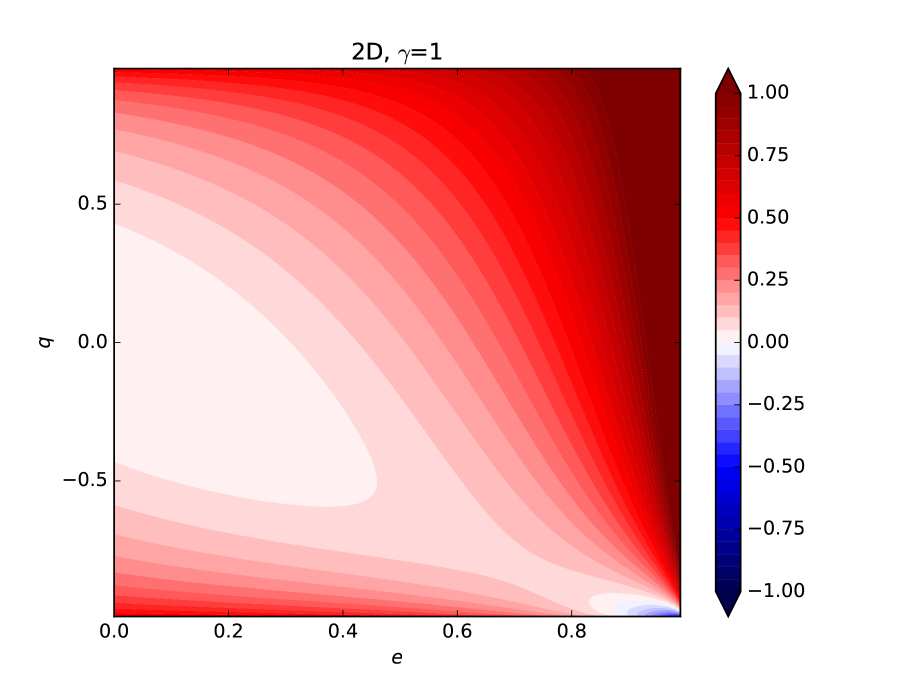
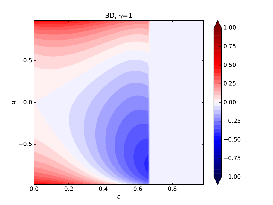
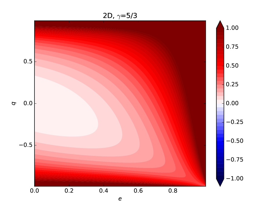
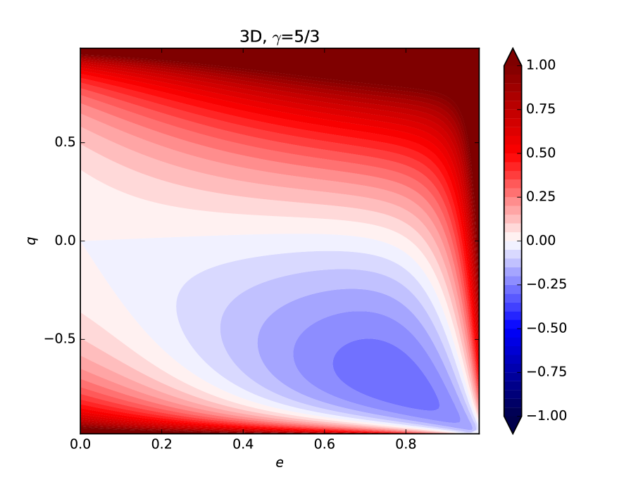
Figure 1: Dimensionless geometric part of the Hamiltonian density for untwisted eccentric discs, as a function of the eccentricity $e$ and the (signed) nonlinearity parameter $q=ae_{a}/[1-e(e+ae_{a})]$. Top left: 2D case for $\gamma=1$. Top right: 3D case for $\gamma=1$. (Values are not plotted for $e>0.66$ because the solution involves extreme compression at periapsis.) Bottom left: 2D case for $\gamma=5/3$, with the additive constant term removed. Bottom right: 3D case for $\gamma=5/3$, with the additive constant term removed.

4 Verification of linear theory

When $e$, $ae_{a}$ and $ae\varpi_{a}$ are much less than unity, the geometric part of the Hamiltonian density for a 2D disc can be approximated as the quadratic function

$$F^{\mathrm{(2D)}}\approx\frac{1}{\gamma-1}+\frac{1}{2}e(e+ae_{a})+\frac{1}{4}\gamma[(ae_{a})^{2}+(ae\varpi_{a})^{2}].$$ (40)

The same expression holds in the isothermal case $\gamma=1$ except that the unimportant constant term is missing. Using this approximation for the Hamiltonian in equations (26) and (27) leads, after some algebra, to the linearized evolutionary equation

$$2\Sigma^{\circ}na^{3}\frac{\partial\mathcal{E}}{\partial t}=\frac{\partial}{\partial a}\left(\mathrm{i}\gamma P^{\circ}a^{3}\frac{\partial\mathcal{E}}{\partial a}\right)+\mathrm{i}\frac{\mathrm{d}P^{\circ}}{\mathrm{d}a}a^{2}\mathcal{E},$$ (41)

where $\mathcal{E}=e\,\mathrm{e}^{\mathrm{i}\varpi}$ is the complex eccentricity, while $\Sigma^{\circ}=M_{a}/2\pi a$ is the surface density of a circular disc with the same mass distribution. This equation is exactly equivalent to equation (21) of Goodchild & Ogilvie (2006) for a 2D adiabatic disc.

In the same linear regime for a 3D disc, an expansion of the ODE (112) leads to the approximations

$$h\approx 1-\frac{3}{\gamma}e\cos E+\frac{(\gamma-1)}{\gamma}(ae_{a}\cos E+ae\varpi_{a}\sin E),$$ (42)

$$F^{\mathrm{(3D)}}\approx\frac{\gamma+1}{2(\gamma-1)}+\frac{1}{4\gamma}\Big{\{}(5\gamma-9\gamma)e^{2}+2(4\gamma-3)eae_{a}\\ +(2\gamma-1)[(ae_{a})^{2}+(ae\varpi_{a})^{2}]\Big{\}}.$$ (43)

This is significantly different from the 2D version and leads instead to the linearized evolutionary equation

$$-2\mathrm{i}\Sigma^{\circ}na^{3}\frac{\partial\mathcal{E}}{\partial t}=\frac{\partial}{\partial a}\left[\left(2-\frac{1}{\gamma}\right)P^{\circ}a^{3}\frac{\partial\mathcal{E}}{\partial a}\right]\\ +\left(4-\frac{3}{\gamma}\right)\frac{\mathrm{d}P^{\circ}}{\mathrm{d}a}a^{2}\mathcal{E}+3\left(1+\frac{1}{\gamma}\right)P^{\circ}a\mathcal{E},$$ (44)

which is exactly equivalent to equation (2) of Teyssandier & Ogilvie (2016) for a 3D adiabatic disc. The last term, in particular, is a prograde contribution to the precession of the disc due to pressure.

The difference between the 2D and 3D theories is most clearly seen in the isothermal case $\gamma=1$, for which

$$F^{\mathrm{(3D)}}=-\langle\ln j\rangle-\langle\ln h\rangle=F^{\mathrm{(2D)}}-\langle\ln h\rangle.$$ (45)

Furthermore, in this case the eccentricity gradient and twist do not affect the vertical oscillation, so $F^{\mathrm{(3D)}}$ separates cleanly into horizontal and vertical parts, where the vertical part depends only on $e$ and has the expansion

$$-\langle\ln h\rangle=-\frac{3}{2}e^{2}+\frac{3}{8}e^{4}+\frac{25}{56}e^{6}+O(e^{8}).$$ (46)

It is a decreasing function of $e$ and so contributes to prograde precession, according to equation (27).

5 Nonlinear eccentric modes

An eccentric mode is a special solution in which the eccentricity distribution $e(a)$ is independent of time and the disc is untwisted and precesses uniformly at angular frequency $\omega$, such that

$$\varpi=\omega t+\mathrm{constant}.$$ (47)

The Hamiltonians we are interested in have the property that $\partial H_{a}/\partial\varpi_{a}=0$ in an untwisted disc with $\varpi_{a}=0$. Therefore equation (26) is automatically satisfied in an eccentric mode, while equation (27) reduces to

$$M_{a}\omega=-\frac{\sqrt{1-e^{2}}}{na^{2}e}\frac{\delta H}{\delta e}.$$ (48)

This is a nonlinear ODE for $e(a)$ in which the precession rate $\omega$ appears as an eigenvalue. In evaluating the right-hand side of this equation, the twist $\varpi_{a}$ can be set to zero.

The modal equation (48) can also be written in the form

$$\omega\frac{\delta L}{\delta e}=\frac{\delta H}{\delta e},$$ (49)

where

$$L=\int M_{a}na^{2}\sqrt{1-e^{2}}\,\mathrm{d}a$$ (50)

is the angular momentum. Note that $L+C=\int na^{2}\,\mathrm{d}M=L^{\circ}$ is a constant property of the disc, being the total angular momentum of a circular disc with the same mass distribution.

The solutions of the modal equation generally involve oscillations of the function $e(a)$, similar to waves on a string. It is conventional in celestial mechanics to regard $e$ as a non-negative quantity and $\varpi$ as being defined modulo $2\pi$ wherever $e\neq 0$. In the case of an untwisted eccentric mode, however, where $e(a)$ may have zeros on particular orbits, it is more convenient to allow $e$ to take both positive and negative values such that $e_{a}$ and $\varpi$ vary continuously. This alternative viewpoint is possible because of the invariance of the equations (and the geometry) when $(e,\varpi)$ are replaced with $(-e,\varpi+\pi)$.

Equation (49) is the Euler–Lagrange equation for the nonlinear variational problem in which we seek stationary values of $H$ subject to the constraint $L=\mathrm{constant}$ (or, equivalently, $C=\mathrm{constant}$). The boundary conditions should be such that either the eccentricity vanishes (a rigid, circular boundary) or $\partial H_{a}/\partial e_{a}=0$ (a free, vacuum boundary). The precession frequency $\omega$ appears here as a Lagrange multiplier. This equation implies that, when the shape of the disc undergoes an infinitesimal change from a modal solution, the infinitesimal changes in $H$ and $L$ are related by $\delta H=\omega\,\delta L$. We expect there to exist multiple branches of modal solutions, along each of which the shape of the mode varies continuously, as do the values of $H$, $L$ and $\omega$. Some or all of these branches will reach the limit of a circular disc in which $H\to H^{\circ}$ and $L\to L^{\circ}$, while $\omega$ tends to a constant value which is the precession rate of the mode in linear theory. Along each branch we expect $H$ and $L$ to be related by $\mathrm{d}H/\mathrm{d}L=\omega$.

When the Hamiltonian density for an untwisted disc is written as $H_{a}=H_{a}^{\circ}F$, where $H_{a}^{\circ}$ depends only on $a$, and $F$ is a dimensionless function of $e$ and $f=e+ae_{a}$, the modal equation can be written explicitly as

$$-\frac{\omega M_{a}}{H_{a}^{\circ}}\frac{na^{2}e}{\sqrt{1-e^{2}}}=\frac{\partial F}{\partial e}-ae_{a}\frac{\partial^{2}F}{\partial e\,\partial f}-a(2e_{a}+ae_{aa})\frac{\partial^{2}F}{\partial f^{2}}\\ -\frac{\mathrm{d}\ln(H_{a}^{\circ})}{\mathrm{d}\ln a}\frac{\partial F}{\partial f}.$$ (51)

We illustrate this theory by considering the case of a 2D disc. We first solve the simple model problem studied by Barker & Ogilvie (2016) in which a 2D isothermal disc is contained within rigid circular boundaries with a radius ratio of $2$. The mass distribution is such that $M_{a}\propto a$, which corresponds to a uniform surface density in the limit of a circular disc. We solve the second-order nonlinear ODE (48) as an eigenvalue problem for the mode frequency $\omega$, using a shooting method. The boundary conditions are $e=0$ at $a=r_{\mathrm{in}}$ and at $a=r_{\mathrm{out}}=2r_{\mathrm{in}}$. We obtain a sequence of modes with increasing numbers of nodes in the eigenfunction $e(a)$ (Fig. 2). The amplitude of the mode can be varied by choosing the value (positive, without loss of generality) of $ae_{a}$ at the inner boundary. As this value approaches its maximum possible value of $1$, the modes become highly nonlinear, with $f=e+ae_{a}$ being close to $\pm 1$ for most values of $a$, and with sharp transitions in between. This means that the modal structures consist of alternating regions in which either the periapses or the apoapses are tightly bunched (Fig. 3).

The variation of the precession rate $\omega$ with the mode amplitude is shown in Fig. 4, along with the variation of the Hamiltonian with the angular-momentum deficit. The precession is retrograde and increases with both amplitude and mode number. The relation $\mathrm{d}H/\mathrm{d}C=-\omega$ (i.e. $\mathrm{d}H/\mathrm{d}L=+\omega$) is verified numerically for each branch. The results for the lowest-order mode agree with those of Barker & Ogilvie (2016), which were obtained by solving a nonlinear ODE for the eccentricity as a function of the semilatus rectum.

When $e+ae_{a}=\pm 1$ we have $ae=\pm a+\mathrm{constant}$. The limiting form of the lowest-order mode is given by

$$ae=\begin{cases}a-r_{\mathrm{in}},&r_{\mathrm{in}}<a<\bar{r},\\ -a+r_{\mathrm{out}},&\bar{r}<a<r_{\mathrm{out}},\end{cases}$$ (52)

where $\bar{r}=(r_{\mathrm{in}}+r_{\mathrm{out}})/2$. It has a finite AMD (equal to $0.02318\,Ml_{\mathrm{in}}$, where $l_{\mathrm{in}}=\sqrt{GM_{1}r_{\mathrm{in}}}$, in the case we have considered), which is the largest AMD that the system can support, and an unbounded Hamiltonian because of the logarithmic divergence (equation 136) as $f\to 1$. The limiting forms of the higher-order modes, which were not considered by Barker & Ogilvie (2016), have similar piecewise linear structures, but the positions of the break points cannot be determined in a straightforward way.

Figure 2: Shapes of nonlinear eccentric modes for the simple model problem considered by Barker & Ogilvie (2016) in which a 2D isothermal disc is contained within rigid circular boundaries with a radius ratio of $2$. The upper two panels show the profiles of $e$ and $f=e+ae_{a}$ for the first four modes with moderately large amplitudes such that $ae_{a}=0.5$ at the inner boundary. The lower panels show the same modes with nearly maximal amplitudes such that $ae_{a}=0.999$ at the inner boundary. Only the lowest-order mode was computed by Barker & Ogilvie (2016).

Figure 3: Shapes of nonlinear eccentric modes for the same problem as in Fig. 2, for the first four modes with nearly maximal amplitudes such that $ae_{a}=0.999$ at the inner boundary.

Figure 4: Left: dependence of the precession frequencies of the families of nonlinear eccentric modes (for the same problem as in Fig. 2) on the mode amplitude, quantified by $e_{\mathrm{max}}=\max|e|$. Here $l_{\mathrm{in}}=\sqrt{GM_{1}r_{\mathrm{in}}}$ is the specific angular momentum of a circular orbit at the inner boundary. Right: Hamiltonian (energy) versus angular-momentum deficit for the same families. The slope of each branch agrees with the negative of the precession frequency. Note that each branch has a limiting value of $C$ at which $H\to\infty$ because an orbital intersection is approached.

We next consider a more realistic problem involving an extended 2D disc with $a_{\mathrm{out}}/a_{\mathrm{in}}=100$ and free boundaries. We also set $\gamma=2$ for this illustrative calculation, and in fact consider a polytrope of index $1$. (As noted above, the geometric Hamiltonian of a 2D disc can be obtained in terms of elementary functions in the cases $\gamma=1$ and $\gamma=2$, which are expected to bracket the range of behaviour expected in a real system.) We take $M_{a}/a\propto\varepsilon^{\circ}\propto T(a)/a$, where $T(a)=\tanh[(a-a_{\mathrm{in}})/w_{\mathrm{in}}]\tanh[(a_{\mathrm{out}}-a)/w_{\mathrm{out}}]$ is a tapering function that is close to $1$ in most of the disc but declines smoothly to $0$ at the inner and outer boundaries over length-scales $w_{\mathrm{in}}=0.01a_{\mathrm{in}}$ and $w_{\mathrm{out}}=0.01a_{\mathrm{out}}$. Apart from the taper, this model corresponds in the circular limit to a surface density $\propto r^{-1}$ and a sound speed $\propto r^{-1/2}$. The free boundary conditions correspond to regularity conditions at $a=a_{\mathrm{in}}$ and $a=a_{\mathrm{out}}$, which are singular points of equation (51). For this model they take the form

$$2a_{\mathrm{in}}\frac{\mathrm{d}T}{\mathrm{d}a}\frac{\partial F}{\partial f}=\frac{\omega na^{2}}{\varepsilon^{\circ}_{\mathrm{in}}}\frac{e}{\sqrt{1-e^{2}}},$$ (53)

where $\varepsilon^{\circ}_{\mathrm{in}}$ is the value of $\varepsilon^{\circ}$ at $a=a_{\mathrm{in}}$ neglecting the taper; this leads to a nonlinear relation between $e$ and $f$ at the boundaries.

The shapes of the first four modes are shown in Fig. 5, where the amplitudes have been chosen such a maximum eccentricity of $0.5$ is attained in each case. Again, the modes form a sequence in which the number of nodes in $e(a)$ increases by one. These modes are less confined than those of the previous problem; with free boundary conditions, $e$ does not need to vanish at the boundaries, and the broad extension of the disc means that the eccentricity gradient can avoid the highly nonlinear limit $f\to 1$ even though $e$ is as large as $0.5$. The precession rate again increases with amplitude and mode number and satisfies the relation $\mathrm{d}H/\mathrm{d}C=-\omega$ (Fig. 6). The numerical values of $-\omega$ in units of $\varepsilon_{\mathrm{in}}/l_{\mathrm{in}}$ are much smaller than the values of $-\omega$ in units of $c_{\mathrm{s}}/l_{\mathrm{in}}$ found in the previous problem (Fig. 4). This is because (i) the eccentricity gradients are more moderate, which reduces the precession rate; (ii) the internal energy in most of the disc is significantly less than $\varepsilon_{\mathrm{in}}$ because of the assumed temperature gradient; and (iii) the majority of the angular momentum is located at $a\gg a_{\mathrm{in}}$.

Figure 5: Same as Fig. 2 for the extended 2D disc with $\gamma=2$, $a_{\mathrm{out}}/a_{\mathrm{in}}=100$ and free boundaries. The amplitudes of the modes are chosen such that $e_{\mathrm{max}}=0.5$.

Figure 6: Same as Fig. 4 for the extended 2D disc with $\gamma=2$, $a_{\mathrm{out}}/a_{\mathrm{in}}=100$ and free boundaries. Here $\varepsilon_{\mathrm{in}}^{\circ}$ is the specific internal energy of a circular disc at the inner boundary, neglecting the taper, and $l_{\mathrm{in}}^{\circ}=\sqrt{GM_{1}a_{\mathrm{in}}}$. Apart from the lowest-order mode, the branches terminate when $e\to 1$ at an interior point.

6 Conclusion

In this paper we have developed a new framework for studying the nonlinear dynamics of eccentric astrophysical discs. In the case of an ideal, non-self-gravitating fluid, a thin eccentric disc consists of a continuous set of nested elliptic orbits that evolve slowly as a result of pressure. The semimajor axis of each orbit is conserved, as is the total angular-momentum deficit of the disc, while the orbits undergo precession and exchanges of eccentricity. The nonlinear dynamics of this system can be derived from a convenient variational principle and expressed in a concise Hamiltonian form, using either canonical (e.g. modified Delaunay) variables or the more familiar Keplerian orbital elements. The Hamiltonian of a 2D disc is just the orbit-averaged internal energy of the disc, which can be determined from its eccentricity distribution using the geometry of the elliptical orbits. In the realistic case of a 3D disc, the Hamiltonian needs to be modified to take into account the dynamical vertical structure of the disc, but is still equal to a multiple of a suitably averaged internal energy.

The simplest solutions of the theory are uniformly precessing nonlinear eccentric modes, which make the Hamiltonian stationary subject to the angular momentum deficit being fixed. We have presented numerical examples of branches of modal solutions in illustrative situations up to their maximum possible amplitudes.

In many astronomical situations of interest, eccentric discs are expected to interact gravitationally with orbital companions; examples include circumbinary discs around young binary stars or binary black holes in galactic nuclei, circumstellar discs in cataclysmic variables and young binary stars, and protoplanetary discs with gap-opening planets. These interactions generally involve both secular effects, which contribute to precession and exchanges of eccentricity between the disc and the companion, and resonant effects, which contribute to the growth or damping of eccentricity. Both have been considered in a linear regime by Goodchild & Ogilvie (2006) and Teyssandier & Ogilvie (2016). It is likely that the Hamiltonian formalism developed here will be useful in understanding the nonlinear dynamics found in long-term simulations by Rosotti et al. (2017) and Ragusa et al. (2018), as it is a description of an ideal fluid that connects more readily with the established methods of celestial mechanics. It may also be helpful in understanding instabilities of eccentric discs that involve mode couplings (Ferreira & Ogilvie, 2008; Kato, 2008; Barker & Ogilvie, 2014). It would be valuable in future to explore further the nonlinear dynamics of 3D eccentric discs using this approach.

The theory developed here is intended to be easier to understand and to use than the nonlinear description of eccentric discs worked out by Ogilvie (2001). The older work considers the eccentricity as a function of semilatus rectum (or angular momentum) rather than semimajor axis (or energy), and requires a number of stress integrals to be computed. The new theory is all derived from a scalar Hamiltonian but does not include dissipative effects. It would be valuable to try to incorporate the effects of viscous dissipation, heating and cooling while preserving as much as possible of the unifying structure of this theory.

Appendix A Derivation of the Hamiltonian form of the equations

In the Hamiltonian theory of dynamics, any canonical transformation from phase-space variables $({\mn@boldsymbol{q}},{\mn@boldsymbol{p}})$ to $({\mn@boldsymbol{Q}},{\mn@boldsymbol{P}})$ satisfies the ‘direct conditions’

$$\frac{\partial P_{i}}{\partial p_{j}}=\frac{\partial q_{j}}{\partial Q_{i}},\qquad\frac{\partial P_{i}}{\partial q_{j}}=-\frac{\partial p_{j}}{\partial Q_{i}},\qquad\frac{\partial Q_{i}}{\partial p_{j}}=-\frac{\partial q_{j}}{\partial P_{i}},\qquad\frac{\partial Q_{i}}{\partial q_{j}}=\frac{\partial p_{j}}{\partial P_{i}}.$$ (54)

We apply these relations with $({\mn@boldsymbol{q}},{\mn@boldsymbol{p}})$ being the Cartesian phase-space coordinates $(x,y,v_{x},v_{y})$ and $({\mn@boldsymbol{Q}},{\mn@boldsymbol{P}})$ being the action–angle variables $(\lambda,\gamma,\Lambda,\Gamma)$. We use the special symbol $\eth$ (rather than $\partial$) to denote partial derivatives of the four-dimensional phase-space transformation $(x,y,v_{x},v_{y})\mapsto(\lambda,\gamma,\Lambda,\Gamma)$ in order to distinguish them from those of the two-dimensional real-space transformation $(x,y)\mapsto(\Lambda,\lambda)$ associated with the orbital coordinate system. Thus, in particular,

$$\frac{\eth\Lambda}{\eth v_{x}}=\frac{\eth x}{\eth\lambda},\qquad\frac{\eth\Lambda}{\eth v_{y}}=\frac{\eth y}{\eth\lambda},\qquad\frac{\eth\Gamma}{\eth v_{x}}=\frac{\eth x}{\eth\gamma},\qquad\frac{\eth\Gamma}{\eth v_{y}}=\frac{\eth y}{\eth\gamma},\qquad\frac{\eth\gamma}{\eth v_{x}}=-\frac{\eth x}{\eth\Gamma},\qquad\frac{\eth\gamma}{\eth v_{y}}=-\frac{\eth y}{\eth\Gamma}.$$ (55)

For a planar system, in the presence of a perturbing force per unit mass ${\mn@boldsymbol{f}}$, the equation of motion of a fluid element or test particle is

$$\dot{v}_{x}=\dots+f_{x},\qquad\dot{v}_{y}=\dots+f_{y},$$ (56)

where the dots represent the Newtonian force due to the central mass. Using the chain rule and the direct conditions, we deduce that the canonical variables that would be constant in a Keplerian orbit evolve according to

$$\dot{\Lambda}=\frac{\eth\Lambda}{\eth v_{x}}f_{x}+\frac{\eth\Lambda}{\eth v_{y}}f_{y}=\frac{\eth x}{\eth\lambda}f_{x}+\frac{\eth y}{\eth\lambda}f_{y},$$ (57)

$$\dot{\Gamma}=\frac{\eth\Gamma}{\eth v_{x}}f_{x}+\frac{\eth\Gamma}{\eth v_{y}}f_{y}=\frac{\eth x}{\eth\gamma}f_{x}+\frac{\eth y}{\eth\gamma}f_{y},$$ (58)

$$\dot{\gamma}=\frac{\eth\gamma}{\eth v_{x}}f_{x}+\frac{\eth\gamma}{\eth v_{y}}f_{y}=-\frac{\eth x}{\eth\Gamma}f_{x}-\frac{\eth y}{\eth\Gamma}f_{y}.$$ (59)

(We will not require $\dot{\lambda}$, which in any case is dominated by the Keplerian mean motion $n$.)

The partial derivatives of the 2D transformation are related to those of the 4D transformation by

$$\frac{\partial x}{\partial\Lambda}=\frac{\eth x}{\eth\Lambda}+\frac{\eth x}{\eth\Gamma}\Gamma_{\Lambda}+\frac{\eth x}{\eth\gamma}\gamma_{\Lambda},\qquad\frac{\partial x}{\partial\lambda}=\frac{\eth x}{\eth\lambda},\qquad\frac{\partial y}{\partial\Lambda}=\frac{\eth y}{\eth\Lambda}+\frac{\eth y}{\eth\Gamma}\Gamma_{\Lambda}+\frac{\eth y}{\eth\gamma}\gamma_{\Lambda},\qquad\frac{\partial y}{\partial\lambda}=\frac{\eth y}{\eth\lambda}.$$ (60)

The Jacobian matrix of the 2D transformation is

$$\begin{pmatrix}\partial x/\partial\Lambda&\partial x/\partial\lambda\\ \partial y/\partial\Lambda&\partial y/\partial\lambda\end{pmatrix},$$ (61)

with determinant

$$J=\frac{\partial x}{\partial\Lambda}\frac{\partial y}{\partial\lambda}-\frac{\partial x}{\partial\lambda}\frac{\partial y}{\partial\Lambda}=\left(\frac{\eth x}{\eth\Lambda}\frac{\eth y}{\eth\lambda}-\frac{\eth x}{\eth\lambda}\frac{\eth y}{\eth\Lambda}\right)+\left(\frac{\eth x}{\eth\Gamma}\frac{\eth y}{\eth\lambda}-\frac{\eth x}{\eth\lambda}\frac{\eth y}{\eth\Gamma}\right)\Gamma_{\Lambda}+\left(\frac{\eth x}{\eth\gamma}\frac{\eth y}{\eth\lambda}-\frac{\eth x}{\eth\lambda}\frac{\eth y}{\eth\gamma}\right)\gamma_{\Lambda}$$ (62)

and inverse

$$\begin{pmatrix}\partial\Lambda/\partial x&\partial\Lambda/\partial y\\ \partial\lambda/\partial x&\partial\lambda/\partial y\end{pmatrix}=\frac{1}{J}\begin{pmatrix}\partial y/\partial\lambda&-\partial x/\partial\lambda\\ -\partial y/\partial\Lambda&\partial x/\partial\Lambda\end{pmatrix}.$$ (63)

For a perturbing force of the form

$${\mn@boldsymbol{f}}=-\frac{1}{\Sigma}{\mn@boldsymbol{\nabla}}P,$$ (64)

where $P$ is a vertically integrated pressure (or other isotropic stress), we deduce that

$$\Sigma\dot{\Lambda}=-\frac{\eth x}{\eth\lambda}\frac{\partial P}{\partial x}-\frac{\eth y}{\eth\lambda}\frac{\partial P}{\partial y},\qquad\Sigma\dot{\Gamma}=-\frac{\eth x}{\eth\gamma}\frac{\partial P}{\partial x}-\frac{\eth y}{\eth\gamma}\frac{\partial P}{\partial y},\qquad\Sigma\dot{\gamma}=\frac{\eth x}{\eth\Gamma}\frac{\partial P}{\partial x}+\frac{\eth y}{\eth\Gamma}\frac{\partial P}{\partial y}.$$ (65)

Using the chain rule on the partial derivatives of $P$ gives

$$\Sigma\dot{\Lambda}=-\frac{\partial P}{\partial\lambda},$$ (66)

$$\Sigma\dot{\Gamma}=-\left(\frac{\eth x}{\eth\gamma}\frac{\partial\Lambda}{\partial x}+\frac{\eth y}{\eth\gamma}\frac{\partial\Lambda}{\partial y}\right)\frac{\partial P}{\partial\Lambda}-\left(\frac{\eth x}{\eth\gamma}\frac{\partial\lambda}{\partial x}+\frac{\eth y}{\eth\gamma}\frac{\partial\lambda}{\partial y}\right)\frac{\partial P}{\partial\lambda},$$ (67)

$$\Sigma\dot{\gamma}=\left(\frac{\eth x}{\eth\Gamma}\frac{\partial\Lambda}{\partial x}+\frac{\eth y}{\eth\Gamma}\frac{\partial\Lambda}{\partial y}\right)\frac{\partial P}{\partial\Lambda}+\left(\frac{\eth x}{\eth\Gamma}\frac{\partial\lambda}{\partial x}+\frac{\eth y}{\eth\Gamma}\frac{\partial\lambda}{\partial y}\right)\frac{\partial P}{\partial\lambda}.$$ (68)

Multiplying by $J$ and using the inverse Jacobian matrix gives

$$J\Sigma\dot{\Lambda}=-J\frac{\partial P}{\partial\lambda},$$ (69)

$$J\Sigma\dot{\Gamma}=-\left(\frac{\eth x}{\eth\gamma}\frac{\partial y}{\partial\lambda}-\frac{\eth y}{\eth\gamma}\frac{\partial x}{\partial\lambda}\right)\frac{\partial P}{\partial\Lambda}-\left(-\frac{\eth x}{\eth\gamma}\frac{\partial y}{\partial\Lambda}+\frac{\eth y}{\eth\gamma}\frac{\partial x}{\partial\Lambda}\right)\frac{\partial P}{\partial\lambda},$$ (70)

$$J\Sigma\dot{\gamma}=\left(\frac{\eth x}{\eth\Gamma}\frac{\partial y}{\partial\lambda}-\frac{\eth y}{\eth\Gamma}\frac{\partial x}{\partial\lambda}\right)\frac{\partial P}{\partial\Lambda}+\left(-\frac{\eth x}{\eth\Gamma}\frac{\partial y}{\partial\Lambda}+\frac{\eth y}{\eth\Gamma}\frac{\partial x}{\partial\Lambda}\right)\frac{\partial P}{\partial\lambda}.$$ (71)

Now we notice from equation (62) that

$$\frac{\partial J}{\partial\Gamma_{\Lambda}}=\frac{\eth x}{\eth\Gamma}\frac{\eth y}{\eth\lambda}-\frac{\eth x}{\eth\lambda}\frac{\eth y}{\eth\Gamma},\qquad\frac{\partial J}{\partial\gamma_{\Lambda}}=\frac{\eth x}{\eth\gamma}\frac{\eth y}{\eth\lambda}-\frac{\eth x}{\eth\lambda}\frac{\eth y}{\eth\gamma}.$$ (72)

Furthermore, we have the differential identities

$$\frac{\partial}{\partial\lambda}\left(\frac{\eth x}{\eth\Gamma}\frac{\partial y}{\partial\Lambda}-\frac{\eth y}{\eth\Gamma}\frac{\partial x}{\partial\Lambda}\right)=\frac{\partial}{\partial\Lambda}\left(\frac{\partial J}{\partial\Gamma_{\Lambda}}\right)-\frac{\partial J}{\partial\Gamma},\qquad\frac{\partial}{\partial\lambda}\left(\frac{\eth x}{\eth\gamma}\frac{\partial y}{\partial\Lambda}-\frac{\eth y}{\eth\gamma}\frac{\partial x}{\partial\Lambda}\right)=\frac{\partial}{\partial\Lambda}\left(\frac{\partial J}{\partial\gamma_{\Lambda}}\right)-\frac{\partial J}{\partial\gamma},$$ (73)

which do not rely on any special properties of the functions $x(\lambda,\gamma,\Lambda,\Gamma)$ and $y(\lambda,\gamma,\Lambda,\Gamma)$. We now carry out an orbital time-average of the equations, denoted by angle brackets:

$$\langle\cdot\rangle=\frac{1}{2\pi}\int_{0}^{2\pi}\cdot\,\mathrm{d}\lambda.$$ (74)

This averaging operation, which also corresponds to a mass-weighted spatial average around the orbit, allows us to integrate by parts with respect to the periodic variable $\lambda$, with the results

$$J\Sigma\langle\dot{\Lambda}\rangle=\left\langle P\frac{\partial J}{\partial\lambda}\right\rangle,$$ (75)

$$J\Sigma\langle\dot{\Gamma}\rangle=-\frac{\partial}{\partial\Lambda}\left\langle P\frac{\partial J}{\partial\gamma_{\Lambda}}\right\rangle+\left\langle P\frac{\partial J}{\partial\gamma}\right\rangle,$$ (76)

$$J\Sigma\langle\dot{\gamma}\rangle=\frac{\partial}{\partial\Lambda}\left\langle P\frac{\partial J}{\partial\Gamma_{\Lambda}}\right\rangle-\left\langle P\frac{\partial J}{\partial\Gamma}\right\rangle.$$ (77)

A.1 2D analysis

In the artificial but widely considered case of a 2D ideal fluid, variations of the vertically integrated pressure $P$ and the specific internal energy $\varepsilon$ around each orbit are adiabatic and related by $\mathrm{d}\varepsilon=-P\,\mathrm{d}A$, where $A=1/\Sigma=(2\pi/M_{\Lambda})J$ is the specific area. The evolutionary equations, multiplied by $2\pi$, then reduce to

$$M_{\Lambda}\langle\dot{\Lambda}\rangle=-M_{\Lambda}\left\langle\frac{\partial\varepsilon}{\partial\lambda}\right\rangle=0,$$ (78)

$$M_{\Lambda}\langle\dot{\Gamma}\rangle=\frac{\partial}{\partial\Lambda}\left(M_{\Lambda}\left\langle\frac{\partial\varepsilon}{\partial\gamma_{\Lambda}}\right\rangle\right)-M_{\Lambda}\left\langle\frac{\partial\varepsilon}{\partial\gamma}\right\rangle,$$ (79)

$$M_{\Lambda}\langle\dot{\gamma}\rangle=-\frac{\partial}{\partial\Lambda}\left(M_{\Lambda}\left\langle\frac{\partial\varepsilon}{\partial\Gamma_{\Lambda}}\right\rangle\right)+M_{\Lambda}\left\langle\frac{\partial\varepsilon}{\partial\Gamma}\right\rangle.$$ (80)

The first equation implies that $\Lambda$, and therefore $a$, is a material invariant in this theory, which is true because there is no dissipation of energy, nor does the pressure transfer any energy between neighbouring orbits. The three equations are in the canonical Hamiltonian form

$$M_{\Lambda}\langle\dot{\Lambda}\rangle=-\frac{\delta H}{\delta\lambda}=0,\qquad M_{\Lambda}\langle\dot{\Gamma}\rangle=-\frac{\delta H}{\delta\gamma},\qquad M_{\Lambda}\langle\dot{\gamma}\rangle=\frac{\delta H}{\delta\Gamma},$$ (81)

where the Hamiltonian $H$ is given by

$$H=\int H_{\Lambda}\,\mathrm{d}\Lambda$$ (82)

with Hamiltonian density

$$H_{\Lambda}=M_{\Lambda}\langle\varepsilon\rangle$$ (83)

involving the orbit-averaged specific internal energy $\langle\varepsilon\rangle$.

A.2 3D analysis

When the third ($z$) dimension perpendicular to the plane of the disc is considered, it can be seen that eccentric discs are never in hydrostatic equilibrium in this vertical direction. A non-zero eccentricity leads to an oscillatory variation of the vertical gravitational acceleration around the orbit, while a non-zero eccentricity gradient or twist leads to an oscillatory horizontal compression of the fluid. In either case the disc undergoes a forced vertical ‘breathing mode’ (Ogilvie, 2001; Ogilvie & Barker, 2014). The differential equation describing the dependence of the vertical scaleheight $H$ around the orbit, for an ideal fluid disc that is stationary in an inertial frame on the orbital timescale, can be written as

$$n^{2}\frac{\partial^{2}H}{\partial\lambda^{2}}+\Psi H=\frac{P}{\Sigma H},$$ (84)

where

$$\Psi=\frac{\partial^{2}\Phi}{\partial z^{2}}\bigg{|}_{z=0}=\frac{GM}{r^{3}}$$ (85)

describes the vertical gravity in a disc (assumed here to be thin), while $P$ and $\Sigma$ are the vertically integrated pressure and density. (Equation 84 is equivalent to equations 141–142 of Ogilvie & Barker (2014).) The mass-weighted vertically averaged specific internal energy of a perfect gas is

$$\bar{\varepsilon}=\int\frac{p}{(\gamma-1)\rho}\,\rho\,\mathrm{d}z\bigg{/}\int\rho\,\mathrm{d}z=\frac{P}{(\gamma-1)\Sigma}.$$ (86)

Adiabatic flow means that $(P/H)\propto(\Sigma/H)^{\gamma}$ around the orbit, so $\mathrm{d}\bar{\varepsilon}=-(P/H)\,\mathrm{d}(AH)$ when $\Lambda$ is held constant.

The associated energy equation is obtained by multiplying equation (84) by $\partial H/\partial\lambda$:

$$\frac{\partial}{\partial\lambda}\left[\frac{1}{2}n^{2}\left(\frac{\partial H}{\partial\lambda}\right)^{2}+\frac{1}{2}\Psi H^{2}+\bar{\varepsilon}\right]=\frac{1}{2}\frac{\partial\Psi}{\partial\lambda}H^{2}-P\frac{\partial A}{\partial\lambda}.$$ (87)

The three terms in the square brackets are the kinetic, gravitational and internal energies per unit mass, after vertical averaging. The two source terms on the right-hand side are due to variable vertical gravity and horizontal orbital compression, respectively. An orbital average gives

$$\left\langle\frac{1}{2}\frac{\partial\Psi}{\partial\lambda}H^{2}-P\frac{\partial A}{\partial\lambda}\right\rangle=0.$$ (88)

On the other hand, multiplying equation (84) by $H$ and averaging (with integration by parts) gives the virial relation

$$\left\langle-n^{2}\left(\frac{\partial H}{\partial\lambda}\right)^{2}+\Psi H^{2}-(\gamma-1)\bar{\varepsilon}\right\rangle=0.$$ (89)

Now consider how the scaleheight responds to variations in the geometry of the disc. Note that, of the two agents driving the vertical oscillation, $\Psi$ depends on $(\Gamma,\gamma)$ as well as $(\Lambda,\lambda)$, while $A$ also depends on $\Gamma_{\Lambda}$ and $\gamma_{\Lambda}$. Consider, for example, variations of $\Gamma$. We differentiate equation (84) with respect to $\Gamma$ to obtain

$$n^{2}\frac{\partial^{3}H}{\partial\lambda^{2}\partial\Gamma}+\frac{\partial\Psi}{\partial\Gamma}H+\Psi\frac{\partial H}{\partial\Gamma}=\frac{P}{\Sigma H}\left[-(\gamma-1)\frac{\partial\ln A}{\partial\Gamma}-\gamma\frac{\partial\ln H}{\partial\Gamma}\right].$$ (90)

We then multiply by $H$ and average (with integration by parts):

$$\left\langle-n^{2}\frac{\partial^{2}H}{\partial\lambda\partial\Gamma}\frac{\partial H}{\partial\lambda}+\frac{\partial\Psi}{\partial\Gamma}H^{2}+\Psi\frac{\partial H}{\partial\Gamma}H\right\rangle=-(\gamma-1)\left\langle P\frac{\partial A}{\partial\Gamma}\right\rangle-\left\langle\frac{\gamma P}{\Sigma H}\frac{\partial H}{\partial\Gamma}\right\rangle.$$ (91)

Using the property

$$\frac{\partial\bar{\varepsilon}}{\partial\Gamma}=-\frac{P}{H}\frac{\partial(AH)}{\partial\Gamma},$$ (92)

we can rearrange to obtain

$$\left\langle\frac{1}{2}\frac{\partial\Psi}{\partial\Gamma}H^{2}-P\frac{\partial A}{\partial\Gamma}\right\rangle=\frac{\partial\mathcal{H}}{\partial\Gamma},$$ (93)

where

$$\mathcal{H}=\left\langle\frac{1}{2}n^{2}\left(\frac{\partial H}{\partial\lambda}\right)^{2}-\frac{1}{2}\Psi H^{2}+\gamma\bar{\varepsilon}\right\rangle.$$ (94)

Using the virial relation, this quantity can be rewritten either as

$$\mathcal{H}=\frac{1}{2}(\gamma+1)\langle\bar{\varepsilon}\rangle,$$ (95)

which is a multiple of the average internal energy, or as

$$\mathcal{H}=\left\langle-\frac{1}{2}n^{2}\left(\frac{\partial H}{\partial\lambda}\right)^{2}+\frac{1}{2}\Psi H^{2}+\bar{\varepsilon}\right\rangle,$$ (96)

which is the average of (potential–kinetic) energy. Indeed, this is (minus) the averaged Lagrangian that appears in the theory of nonlinear dispersive waves (Whitham, 1965).

It can be shown similarly that

$$\left\langle\frac{1}{2}\frac{\partial\Psi}{\partial\gamma}H^{2}-P\frac{\partial A}{\partial\gamma}\right\rangle=\frac{\partial\mathcal{H}}{\partial\gamma}.$$ (97)

When the additional horizontal gravitational force (with mass-weighted vertical averaging) due to $\Psi$ is added to the evolutionary equations, we have

$$J\Sigma\langle\dot{\Lambda}\rangle=\left\langle P\frac{\partial J}{\partial\lambda}\right\rangle-J\Sigma\left\langle\frac{1}{2}\frac{\partial\Psi}{\partial\lambda}H^{2}\right\rangle,$$ (98)

$$J\Sigma\langle\dot{\Gamma}\rangle=-\frac{\partial}{\partial\Lambda}\left\langle P\frac{\partial J}{\partial\gamma_{\Lambda}}\right\rangle+\left\langle P\frac{\partial J}{\partial\gamma}\right\rangle-J\Sigma\left\langle\frac{1}{2}\frac{\partial\Psi}{\partial\gamma}H^{2}\right\rangle,$$ (99)

$$J\Sigma\langle\dot{\gamma}\rangle=\frac{\partial}{\partial\Lambda}\left\langle P\frac{\partial J}{\partial\Gamma_{\Lambda}}\right\rangle-\left\langle P\frac{\partial J}{\partial\Gamma}\right\rangle+J\Sigma\left\langle\frac{1}{2}\frac{\partial\Psi}{\partial\Gamma}H^{2}\right\rangle.$$ (100)

Using equations (88), (93) and (97), we see that $\langle\dot{\Lambda}\rangle$ evaluates to zero, and that the equations are of Hamiltonian form, with Hamiltonian density given by

$$H_{\Lambda}=M_{\Lambda}\mathcal{H}=\frac{1}{2}(\gamma+1)M_{\Lambda}\langle\bar{\varepsilon}\rangle.$$ (101)

Appendix B Dimensionless forms of the Hamiltonian density

B.1 2D analysis

For a perfect gas of adiabatic index $\gamma$, adiabatic flow around each orbit means that $P=K\Sigma^{\gamma}$, where $K(a)$ is related to the entropy distribution, which does not evolve. The specific internal energy is then

$$\varepsilon=\frac{P}{(\gamma-1)\Sigma}=\frac{K\Sigma^{\gamma-1}}{\gamma-1}.$$ (102)

Recall that equation (15) relates the surface density $\Sigma$ to the mass distribution $M_{\Lambda}$ and the Jacobian $J=J^{\circ}j$. If the disc had the same distributions of mass and entropy but were circular, it would have $\Sigma=\Sigma^{\circ}=M_{\Lambda}/2\pi J^{\circ}$ and $P=P^{\circ}=K(\Sigma^{\circ})^{\gamma}$. Thus $\Sigma=\Sigma^{\circ}j^{-1}$ and

$$H_{a}=M_{a}\langle\varepsilon\rangle=H^{\circ}_{a}F^{\mathrm{(2D)}},$$ (103)

where

$$H^{\circ}_{a}=2\pi aP^{\circ}$$ (104)

is a given function of $a$ and

$$F^{\mathrm{(2D)}} =\frac{1}{\gamma-1}\left\langle j^{-(\gamma-1)}\right\rangle$$

$$=\left(\frac{1}{\gamma-1}\right)\frac{1}{2\pi}\int_{0}^{2\pi}\left[\frac{1-e(e+ae_{a})}{\sqrt{1-e^{2}}}-\frac{ae_{a}\cos E}{\sqrt{1-e^{2}}}-ae\varpi_{a}\sin E\right]^{-(\gamma-1)}(1-e\cos E)\,\mathrm{d}E$$ (105)

is the dimensionless, geometric part of the Hamiltonian density, which depends on $e$, $ae_{a}$, $ae\varpi_{a}$ and $\gamma$.

In the case of a (globally) isothermal disc we instead have

$$\varepsilon=c_{\mathrm{s}}^{2}\ln\Sigma+\mathrm{constant},$$ (106)

where $c_{\mathrm{s}}=\mathrm{constant}$ is the isothermal sound speed. Then

$$H_{a}=M_{a}\langle\varepsilon\rangle=H^{\circ}_{a}\left(\ln\Sigma^{\circ}+\mathrm{constant}+F^{\mathrm{(2D)}}\right),$$ (107)

where

$$H^{\circ}_{a}=M_{a}c_{\mathrm{s}}^{2}=2\pi aP^{\circ}$$ (108)

and

$$F^{\mathrm{(2D)}}=-\langle\ln j\rangle=-\frac{1}{2\pi}\int_{0}^{2\pi}\ln\left[\frac{1-e(e+ae_{a})}{\sqrt{1-e^{2}}}-\frac{ae_{a}\cos E}{\sqrt{1-e^{2}}}-ae\varpi_{a}\sin E\right](1-e\cos E)\,\mathrm{d}E.$$ (109)

This expression agrees with the limit $\gamma\to 1$ of equation (105) after the constant term $1/(\gamma-1)$ (which, like the terms depending only on $a$ in equation 107, does not affect the dynamics) is removed from it. This follows from the result

$$\lim_{\gamma\to 1}\frac{j^{-(\gamma-1)}-1}{\gamma-1}=-\ln j.$$ (110)

B.2 3D analysis

For a 3D disc, adiabatic flow means instead that $(P/H)=K(\Sigma/H)^{\gamma}$, where $K$ is a fixed function of $a$. If we write the scaleheight as $H=H^{\circ}(a)h(E)$, where $H^{\circ}=(P^{\circ}/\Sigma^{\circ}n^{2})^{1/2}$ is the (hydrostatic) vertical scaleheight of a circular disc with the same mass and entropy distributions, then we have $\Sigma=\Sigma^{\circ}j^{-1}$ and $P=P^{\circ}j^{-\gamma}h^{-(\gamma-1)}$. Equation (84) reduces to a dimensionless ODE for the dimensionless scaleheight $h$:

$$\frac{\mathrm{d}^{2}h}{\mathrm{d}\lambda^{2}}+\frac{h}{(1-e\cos E)^{3}}=\frac{1}{j^{\gamma-1}h^{\gamma}},$$ (111)

or, in terms of derivatives with respect to the eccentric anomaly,

$$(1-e\cos E)\frac{\mathrm{d}^{2}h}{\mathrm{d}E^{2}}-e\sin E\frac{\mathrm{d}h}{\mathrm{d}E}+h=\frac{(1-e\cos E)^{3}}{j^{\gamma-1}h^{\gamma}}.$$ (112)

We then have the Hamiltonian density

$$H_{a}=\frac{1}{2}(\gamma+1)M_{a}\langle\bar{\varepsilon}\rangle=H_{a}^{\circ}F^{\mathrm{(3D)}},$$ (113)

with

$$H_{a}^{\circ}=2\pi aP^{\circ}$$ (114)

and

$$F^{\mathrm{(3D)}}=\frac{(\gamma+1)}{2(\gamma-1)}\left\langle(jh)^{-(\gamma-1)}\right\rangle.$$ (115)

In the isothermal case we have instead

$$\bar{\varepsilon}=c_{\mathrm{s}}^{2}\ln\left(\frac{\Sigma}{H}\right)+\mathrm{constant},$$ (116)

$$H_{a}=M_{a}\langle\bar{\varepsilon}\rangle=H_{a}^{\circ}\left(\ln\Sigma^{\circ}-\ln H^{\circ}+\mathrm{constant}+F^{\mathrm{(3D)}}\right),$$ (117)

$$F^{\mathrm{(3D)}}=-\langle\ln(jh)\rangle.$$ (118)

Appendix C Analaytical expressions for the Hamiltonian of a 2D disc

The quantity $j$ in square brackets in equation (105) or (109) can be written as

$$j=\frac{1-e(e+ae_{a})}{\sqrt{1-e^{2}}}(1-q\cos\theta),$$ (119)

where $\theta=E-\alpha$, with the amplitude $q$ and phase $\alpha$ satisfying

$$q\cos\alpha=\frac{ae_{a}}{1-e(e+ae_{a})},\qquad q\sin\alpha=\frac{\sqrt{1-e^{2}}\,ae\varpi_{a}}{1-e(e+ae_{a})},$$ (120)

which implies

$$q^{2}=\frac{(ae_{a})^{2}+(1-e^{2})(ae\varpi_{a})^{2}}{[1-e(e+ae_{a})]^{2}},\qquad 1-q^{2}=\frac{(1-e^{2})[1-(e+ae_{a})^{2}-(ae\varpi_{a})^{2}]}{[1-e(e+ae_{a})]^{2}},\qquad\tan\alpha=\frac{\sqrt{1-e^{2}}\,e\varpi_{a}}{e_{a}}.$$ (121)

To avoid orbital intersection we require $|q|<1$. In the untwisted case $\varpi_{a}=0$ it is natural to take $\alpha=0$ and regard $q$ as a signed quantity. $q$ is a measure of the degree of areal compression and the level of nonlinearity in an eccentric disc; it generalizes the nonlinearity parameter used in the theory of planetary rings in the regime $e\ll 1$.

For general $\gamma$ the integral (105) can be evaluated in terms of Legendre functions. The special case $\gamma=2$ and the limiting isothermal case $\gamma=1$ involve only elementary functions.

Let

$$I_{p}(q)=\frac{1}{2\pi}\int_{0}^{2\pi}\frac{\mathrm{d}\theta}{(1-q\cos\theta)^{p}}$$ (122)

for $|q|<1$. This is an even function of $q$ with $I_{p}(0)=1$. For $p>0$ or $p<-1$ it is a monotonically increasing function of $q$ for $0<q<1$. For $p>1/2$ it diverges proportionally to $(1-q)^{(1/2)-p}$ as $q\to 1$. For $-1<p<0$ it is monotonically decreasing. For $p=0$ or $p=-1$ it is constant and equal to $1$. Special cases include

$$I_{-1}(q)=1,\qquad I_{0}(q)=1,\qquad I_{1}(q)=(1-q^{2})^{-1/2},\qquad I_{2}(q)=(1-q^{2})^{-3/2}.$$ (123)

In general, $I_{p}(q)$ can be written in terms of the Legendre function:

$$I_{p}(q)=z^{p}P_{p-1}(z),\qquad z=\frac{1}{\sqrt{1-q^{2}}}.$$ (124)

A series expansion, convergent for all $|q|<1$, is

$$I_{p}(q)=\sum_{n=0}^{\infty}\binom{p+2n-1}{2n}J_{n}q^{2n},$$ (125)

where

$$J_{n}=\frac{1}{2\pi}\int_{0}^{2\pi}\cos^{2n}\theta\,\mathrm{d}\theta=\frac{(2n)!}{2^{2n}(n!)^{2}},$$ (126)

which behaves as

$$J_{n}\sim\frac{1}{\sqrt{\pi n}}\qquad\hbox{as $n\to\infty$}.$$ (127)

Thus

$$I_{p}(q)=\sum_{n=0}^{\infty}\frac{(p+2n-1)(p+2n-2)\cdots p}{2^{2n}(n!)^{2}}\,q^{2n}.$$ (128)

To express the integral (105) in terms of $I_{p}(q)$, we use equation (119) and change variables from $E$ to $\theta$. Note that

$$\frac{1}{2\pi}\int_{0}^{2\pi}\frac{\cos\theta\,\mathrm{d}\theta}{(1-q\cos\theta)^{p}}=\frac{I_{p}(q)-I_{p-1}(q)}{q},\qquad\frac{1}{2\pi}\int_{0}^{2\pi}\frac{\sin\theta\,\mathrm{d}\theta}{(1-q\cos\theta)^{p}}=0.$$ (129)

Thus, for $\gamma>1$,

$$F^{\mathrm{(2D)}}=\frac{1}{\gamma-1}\left[\frac{\sqrt{1-e^{2}}}{1-e(e+ae_{a})}\right]^{\gamma-1}[(1-x)I_{\gamma-1}(q)+xI_{\gamma-2}(q)],$$ (130)

with

$$x=\frac{e\cos\alpha}{q}=\frac{eae_{a}}{q^{2}[1-e(e+ae_{a})]}=\frac{eae_{a}[1-e(e+ae_{a})]}{(ae_{a})^{2}+(1-e^{2})(ae\varpi_{a})^{2}}.$$ (131)

When $\gamma=2$ we have a result in terms of elementary functions:

$$F^{\mathrm{(2D)}}=\frac{\sqrt{1-e^{2}}}{1-e(e+ae_{a})}\left(\frac{1-x}{\sqrt{1-q^{2}}}+x\right).$$ (132)

In the untwisted case this reduces to

$$F^{\mathrm{(2D)}}=\frac{1}{(f-e)}\left[\frac{(1+e^{2})f-2e}{\sqrt{1-f^{2}}}+e\sqrt{1-e^{2}}\right],$$ (133)

where $f=e+ae_{a}$.

For the isothermal case $\gamma=1$ we use instead

$$\frac{1}{2\pi}\int_{0}^{2\pi}\ln(1-q\cos\theta)\,\mathrm{d}\theta=\ln\left(\frac{{\textstyle\frac{1}{2}}q^{2}}{1-\sqrt{1-q^{2}}}\right),\qquad\frac{1}{2\pi}\int_{0}^{2\pi}\cos\theta\,\ln(1-q\cos\theta)\,\mathrm{d}\theta=-\left(\frac{1-\sqrt{1-q^{2}}}{q}\right),$$ (134)

leading to

$$F^{\mathrm{(2D)}}=\ln\left[\frac{2\sqrt{1-e^{2}}\left(1-\sqrt{1-q^{2}}\right)}{q^{2}[1-e(e+ae_{a})]}\right]-\frac{eae_{a}\left(1-\sqrt{1-q^{2}}\right)}{q^{2}[1-e(e+ae_{a})]}.$$ (135)

In the untwisted case this reduces to

$$F^{\mathrm{(2D)}}=\ln\left[\frac{2\sqrt{1-e^{2}}\left(1-ef-\sqrt{1-e^{2}}\sqrt{1-f^{2}}\right)}{(f-e)^{2}}\right]-\left(\frac{e}{f-e}\right)\left(1-ef-\sqrt{1-e^{2}}\sqrt{1-f^{2}}\right).$$ (136)

The apparent singularities at $e=f$ in the untwisted expressions can be removed by using the trigonometric parametrization $e=\sin 2\alpha$, $f=\sin 2\beta$, $\sqrt{1-e^{2}}=\cos 2\alpha$, $\sqrt{1-f^{2}}=\cos 2\beta$. This leads to

$$F^{\mathrm{(2D)}}=\frac{1}{2}\sec 2\beta\sec(\alpha+\beta)[3\cos(\alpha+\beta)-\cos(3\alpha-\beta)]$$ (137)

for $\gamma=2$ and

$$F^{\mathrm{(2D)}}=\ln\cos 2\alpha-2\ln\cos(\alpha+\beta)+\sin 2\alpha\sin(\alpha-\beta)\sec(\alpha+\beta)$$ (138)

for $\gamma=1$.

References

- Artymowicz & Lubow (1996) Artymowicz P., Lubow S. H., 1996, ApJ, 467, L77
- Barker & Ogilvie (2014) Barker A. J., Ogilvie G. I., 2014, MNRAS, 445, 2637
- Barker & Ogilvie (2016) Barker A. J., Ogilvie G. I., 2016, MNRAS, 458, 3739
- Bonnerot et al. (2016) Bonnerot C., Rossi E. M., Lodato G., Price D. J., 2016, MNRAS, 455, 2253
- Borderies, Goldreich & Tremaine (1983) Borderies N., Goldreich P., Tremaine S., 1983, AJ, 88, 1560
- Cao et al. (2018) Cao R., Liu F. K., Zhou Z. Q., Komossa S., Ho L. C., 2018, MNRAS, in press
- Cauley et al. (2018) Cauley P. W., Farihi J., Redfield S., Bachman S., Parsons S. G., Gänsicke B. T., 2018, ApJ, 852, L22
- D’Angelo, Lubow & Bate (2006) D’Angelo G., Lubow S. H., Bate M. R., 2006, ApJ, 652, 1698
- Duffell & Chiang (2015) Duffell P. C., Chiang E., 2015, ApJ, 812, 94
- Ferreira & Ogilvie (2008) Ferreira B. T., Ogilvie G. I., 2008, MNRAS, 386, 2297
- Fu, Lubow & Martin (2015a) Fu W., Lubow S. H., Martin R. G., 2015a, ApJ, 807, 75
- Fu, Lubow & Martin (2015b) Fu W., Lubow S. H., Martin R. G., 2015b, ApJ, 813, 105
- Goldreich & Sari (2003) Goldreich P., Sari R., 2003, ApJ, 585, 1024
- Goldreich & Tremaine (1981) Goldreich P., Tremaine S., 1981, ApJ, 243, 1062
- Goodchild & Ogilvie (2006) Goodchild S., Ogilvie G., 2006, MNRAS, 368, 1123
- Guillochon, Manukian & Ramirez-Ruiz (2014) Guillochon J., Manukian H., Ramirez-Ruiz E., 2014, ApJ, 783, 23
- Kato (2008) Kato S., 2008, PASJ, 60, 111
- Kley & Dirksen (2006) Kley W., Dirksen G., 2006, A&A, 447, 369
- Kley, Papaloizou & Ogilvie (2008) Kley W., Papaloizou J. C. B., Ogilvie G. I., 2008, A&A, 487, 671
- Laskar (1997) Laskar J., 1997, A&A, 317, L75
- Lubow (1991a) Lubow S. H., 1991a, ApJ, 381, 259
- Lubow (1991b) Lubow S. H., 1991b, ApJ, 381, 268
- Lubow & Ogilvie (2017) Lubow S. H., Ogilvie G. I., 2017, MNRAS, 469, 4292
- MacFadyen & Milosavljević (2008) MacFadyen A. I., Milosavljević M., 2008, ApJ, 672, 83-93
- Manser et al. (2016) Manser C. J., Gänsicke B. T., Koester D., Marsh T. R., Southworth J., 2016, MNRAS, 462, 1461
- Martin et al. (2014) Martin R. G., Nixon C., Lubow S. H., Armitage P. J., Price D. J., Doğan S., King A., 2014, ApJ, 792, L33
- Miranda, Muñoz & Lai (2017) Miranda R., Muñoz D. J., Lai D., 2017, MNRAS, 466, 1170
- Miranda & Rafikov (2018) Miranda R., Rafikov R. R., 2018, ApJ, 857, 135
- Ogilvie (2001) Ogilvie G. I., 2001, MNRAS, 325, 231
- Ogilvie (2008) Ogilvie G. I., 2008, MNRAS, 388, 1372
- Ogilvie & Barker (2014) Ogilvie G. I., Barker A. J., 2014, MNRAS, 445, 2621
- Papaloizou (2002) Papaloizou J. C. B., 2002, A&A, 388, 615
- Papaloizou, Nelson & Masset (2001) Papaloizou J. C. B., Nelson R. P., Masset F., 2001, A&A, 366, 263
- Ragusa et al. (2018) Ragusa E., Rosotti G., Teyssandier J., Booth R., Clarke C. J., Lodato G., 2018, MNRAS, 474, 4460
- Rosotti et al. (2017) Rosotti G. P., Booth R. A., Clarke C. J., Teyssandier J., Facchini S., Mustill A. J., 2017, MNRAS, 464, L114
- Rice, Armitage & Hogg (2008) Rice W. K. M., Armitage P. J., Hogg D. F., 2008, MNRAS, 384, 1242
- Smith et al. (2007) Smith A. J., Haswell C. A., Murray J. R., Truss M. R., Foulkes S. B., 2007, MNRAS, 378, 785
- Statler (2001) Statler T. S., 2001, AJ, 122, 2257
- Teyssandier & Ogilvie (2016) Teyssandier J., Ogilvie G. I., 2016, MNRAS, 458, 3221
- Teyssandier & Ogilvie (2017) Teyssandier J., Ogilvie G. I., 2017, MNRAS, 467, 4577
- Thun, Kley & Picogna (2017) Thun D., Kley W., Picogna G., 2017, A&A, 604, A102
- Whitehurst (1988) Whitehurst R., 1988, MNRAS, 232, 35
- Whitham (1965) Whitham G. B., 1965, J. Fluid Mech., 22, 273
- Zanazzi & Lai (2017) Zanazzi J. J., Lai D., 2017, MNRAS, 467, 1957