First-principles theory of spatial dispersion: Dynamical quadrupoles and flexoelectricity

Abstract

Density-functional perturbation theory (DFPT) is nowadays the method of choice for the accurate computation of linear and non-linear response properties of materials from first principles. A notable advantage of DFPT over alternative approaches is the possibility of treating incommensurate lattice distortions with an arbitrary wavevector, ${\bf q}$, at essentially the same computational cost as the lattice-periodic case. Here we show that ${\bf q}$ can be formally treated as a perturbation parameter, and used in conjunction with established results of perturbation theory (e.g. the “$2n+1$” theorem) to perform a long-wave expansion of an arbitrary response function in powers of the wavevector components. This provides a powerful, general framework to accessing a wide range of spatial dispersion effects that were formerly difficult to calculate by means of first-principles electronic-structure methods. In particular, the physical response to the spatial gradient of any external field can now be calculated at negligible cost, by using the response functions to uniform perturbations (electric, magnetic or strain fields) as the only input. We demonstrate our method by calculating the flexoelectric and dynamical quadrupole tensors of selected crystalline insulators and model systems.

I Introduction

Spatial dispersion refers to a dependence of a material property (e.g. permittivity, conductivity or phonon frequency) on the wavevector ${\bf q}$ at which it is probed, or equivalently on the gradients of the perturbation and/or the response in real space. Its origin can be traced back to the nonlocality of the microscopic interactions in condensed-matter systems, where the response to an external field (electromagnetic field or atomic displacement) typically occurs over a neighborhood of the point where the field is applied. While in general such effects are weak and can often be neglected in macroscopic theories, there are several instances where their physical consequences are important, both regarding their fundamental interest and their potential towards practical applications. Indeed, with the ongoing interest in nanoscale phenomena, researchers are increasingly often facing situations where the relevant scalar, vector or tensor quantities (e.g. polarization or strain) display large variations on a very small length scale; this is precisely the regime at which gradient effects can become strong.

Historically, spatial dispersion has been most studied in the context of the optical response. The first-order wavevector dependence of the dielectric susceptibility tensor, for example, is responsible for the natural optical activity, Malashevich and Souza (2010); Prosandeev et al. (2013) which is the property of some crystals of rotating the plane of polarization of the transmitted light. Manifestations of spatial dispersion are, however, ubiquitous; they can involve magnetism (the magnetoelectric effect can be regarded as the first-order dispersion of the conductivity Malashevich and Souza (2010)) or elastic degrees of freedom as well (the counterpart of optical gyrotropy in phononics is known as acoustical activity Portigal and Burstein (1968)). In the latter context, flexoelectricity Tagantsev (1986) is arguably the most notable example, as it has been intensely explored both experimentally and theoretically in the past ten years or so. Zubko et al. (2013); Stengel and Vanderbilt (2016) It describes the polarization response to the gradient of the applied strain, and therefore it can be understood as the spatial dispersion of the piezoelectric tensor. Being it a universal property of all insulators regardless of crystal symmetry, it provides a tantalizing route to novel electromechanical device concepts, Bhaskar et al. (2016) and opens the way to many other applications in energy and information technology. Lu et al. (2012); Narvaez et al. (2016)

The long-wavelength regime also occupies a central place in the theory of lattice dynamics in insulators. Indeed, in the ${\bf q}\rightarrow 0$ limit, phonons in insulating crystals are associated with macroscopic electric fields that are due to the long-range electrostatic interactions between atoms. Born and Huang (1954) Identifying and correctly treating such long-range contributions is crucial for a meaningful calculation of the interatomic force constants (IFC) from first principles. Gonze and Lee (1997); Baroni et al. (2001) The former are typically written as electrostatic dipole-dipole terms, which are responsible for the well-known frequency splitting between longitudinal (LO) and transverse (TO) optical phonon branches. It is important to note, however, that the dipole-dipole term only captures the leading contribution to the long-range IFCs. (Dipole-dipole terms decay as $1/d^{3}$ as a function of the interatomic distance, $d$.) Higher orders ($1/d^{4}$ and faster) are always present, but are systematically neglected as their physical consequences are much more subtle.

The next lowest order, for example, involves dipole-quadrupole interactions and is responsible for a nonanalytic behavior Stengel (2013a) of the force-constant matrix at $\mathcal{O}(q^{1})$; this translates into a $1/d^{4}$ decay in real space of the corresponding contribution to the IFCs. A quadrupolar response to an atomic displacement requires a broken-inversion symmetry environment to be active, and is always (although not exclusively) present in piezoelectric crystals. Interestingly, in his seminal 1972 paper, R.M. Martin predicted Martin (1972) that the electronic contribution to the piezoelectric tensor can be written as a sublattice sum of the “dynamical quadrupoles”, so we expect these couplings to be important in compounds where electromechanical effects are strong. However, viable methods to compute the quadrupole tensor have been lacking to date; this quantity can be regarded as the first-order spatial dispersion of the Born effective charge tensor, and is therefore characterized by analogous technical challenges as the calculation of the flexoelectric tensor.

Developing a systematic, quantitative theory of such effects would be very desirable to improve their fundamental understanding and support the ongoing experimental efforts. Achieving this goal, however, presents considerable technical difficulties from the point of view of first-principles electronic-structure theory, due to the inherent breakdown of translational periodicity that a spatial gradient entails. In the case of flexoelectricity, for example, several routes have been explored to cope with this issue. Initially, the flexoelectric coefficients were written as real-space moments of the response (either the electronic charge density or the atomic forces) to the displacement of an isolated atom Hong and Vanderbilt (2011, 2013). Later, the real-space sums were recast as small-${\bf q}$ expansions of the response to a monochromatic displacement pattern at a given wavevector ${\bf q}$. Stengel (2013a, b, 2014) Other subtleties were addressed as well, such as the definition and implementation of the current-density response, Dreyer et al. (2018) which eventually allowed for the calculation of the bulk flexoelectric tensor within a perturbative framework based on a primitive cell of the crystal. Dreyer et al. (2018)

While the strategy of Ref. Dreyer et al., 2018 could be, in principle, generalized to other physical properties, it still presents an important drawback. Several linear-response calculations need to be performed at different ${\bf q}$-points in a vicinity of the Brillouin zone center, and the second-order coefficients (corresponding to the flexoelectric tensor components) are then extracted via a numerical fit. This introduces a significant computational overhead (to repeat the same calculations at several values of ${\bf q}$), and is a potential source of numerical inaccuracies related to the fit. It would be much cheaper from the computational point of view, and convenient from the point of view of the end user, to directly calculate the desired dispersion coefficients as part of the intrinsic linear-response capabilities of the code. To achieve this goal, however, one needs first to establish a general formalism to describing the long-wavelength limit within the context of DFPT.

Here we provide a comprehensive solution to the above issues by first rewriting the second-order energy at finite ${\bf q}$ as an unconstrained minimization problem of a variational functional of the first-order wavefunctions. Next, we show that the parametric ${\bf q}$-dependence of the second-order energy can be regarded as a small perturbation of the ${\bf q}=0$ functional; hence, one can apply the standard tools of DFPT to perform an analytic long-wavelength expansion of an arbitrary response property of the crystal in powers of ${\bf q}$. Remarkably this strategy, in combination with the “$2n+1$” theorem, enables writing explicit formulas for first-order dispersion coefficients that only need the uniform field wavefunction response as an input. Thus, one can take advantage of the already implemented linear-response tools to calculate a wide range of new materials properties, such as flexoelectricity and the natural optical activity, at essentially no cost – and without the need for explicitly implementing or calculating the wavefunction response to a gradient of the external field. Finally, we demonstrate our formalism by implementing the formulas for the clamped-ion flexoelectric coefficients and the dynamical quadrupole tensor (the higher-order multipolar counterpart of the Born dynamical charge tensor). The flexoelectric coefficients calculated for several materials are consistent with previously published results. Stengel (2014); Dreyer et al. (2018) The relationship, established by R. M. Martin in his seminal paper, Martin (1972) between the sublattice sum of the quadrupole moments and the clamped-ion piezoelectric coefficients is numerically verified to a high degree of accuracy. Both quantities converge with respect to plane-wave cutoff and ${\bf k}$-mesh density comparably fast to “standard” linear-response properties (e.g. the macroscopic dielectric tensor), and can now be obtained in a tiny fraction of the computational burden that was formerly needed.

This work is organized as follows. In Section II we present our method, based on the long-wavelength expansion of DFPT, and provide general formulas for dispersion properties at the lowest orders in ${\bf q}$. In Section III we discuss the finite-${\bf q}$ generalization of the electric-field response, which we shall use to define and compute the polarization response in the long-wavelength limit. In Sections IV and V we demonstrate our long-wave approach by deriving and calculating the dynamical quadrupole and clamped-ion flexoelectric tensors in selected materials and model systems. Finally, in Section VI we present our conclusions and outlook, e.g. regarding future generalizations of our method to other dispersion properties. The Appendices provide additional analytic support to the formulas reported in the main text.

II Long-wave perturbation theory

II.1 Density-functional perturbation theory

Here we shall briefly introduce the basic principles of DFPT, both for completeness and in order to support the formal developments of the later sections. Consider an external perturbation to the electronic ground state, which we describe by assuming a parametric dependence of the Hamiltonian operator on a small parameter $\lambda$,

$$\hat{H}(\lambda)=\hat{H}^{(0)}+\lambda\hat{H}^{(1)}+\lambda^{2}\hat{H}^{(2)}+\cdots.$$ (1)

The linear response of the wavefunctions to the perturbation can be recast in terms of a Sternheimer equation,

$$\hat{Q}\left(H^{(0)}-\epsilon^{(0)}_{m}\right)\hat{Q}|\psi^{(1)}_{m}\rangle=-\hat{Q}\hat{\mathcal{H}}^{(1)}|\psi^{(0)}_{m}\rangle,$$ (2)

where $\hat{Q}$ indicates the projector on the unoccupied band manifold, and

$$\hat{\mathcal{H}}^{(1)}=\hat{H}^{(1)}+\hat{V}^{(1)}$$ (3)

contains, in addition to the external perturbation $\hat{H}^{(1)}$, the self-consistent (SCF) potential response, $\hat{V}^{(1)}$, that depends on the first-order electron density as

$$V^{(1)}({\bf r}) = \int d^{3}r^{\prime}\,K_{\rm Hxc}({\bf r,r^{\prime}})n^{(1)}({\bf r}),$$ (4)

$$n^{(1)}({\bf r}) = 2\Re\,\sum_{m}\langle\psi^{(0)}_{m}|{\bf r}\rangle\langle{\bf r}|\psi^{(1)}_{m}\rangle.$$ (5)

$K_{\rm Hxc}({\bf r,r^{\prime}})$ is the Hartree, exchange and correlation (Hxc) kernel, which is defined as the variation of the SCF potential at ${\bf r}$ with respect to a charge density perturbation at ${\bf r}^{\prime}$, calculated at the ground-state density ${n^{(0)}}$,

$$K_{\rm Hxc}({\bf r,r^{\prime}})=\frac{\delta V_{\rm Hxc}({\bf r})}{\delta n({\bf r}^{\prime})}\Big{|}_{n^{(0)}}=\frac{\delta^{2}E_{\rm Hxc}}{\delta n({\bf r})\delta n({\bf r}^{\prime})}\Big{|}_{n^{(0)}}.$$ (6)

The second-order variation of the energy with respect to the perturbation can be then written as

$$E^{(2)}=\sum_{m}\langle\psi^{(0)}_{m}|\hat{H}^{(1)}|\psi^{(1)}_{m}\rangle+\frac{1}{2}\frac{\partial^{2}E}{\partial\lambda^{2}},$$ (7)

where the second term on the right-hand side does not depend on the first-order wavefunctions,

$$\frac{1}{2}\frac{\partial^{2}E}{\partial\lambda^{2}}=\sum_{m}\langle\psi^{(0)}_{m}|\hat{H}^{(2)}|\psi^{(0)}_{m}\rangle.$$ (8)

One can also recast the linear-response problem as a variational functional of the first-order wavefunctions, Gonze (1995a)

$$E^{(2)} = \sum_{m}\langle\psi^{(1)}_{m}|\left(H^{(0)}-\epsilon^{(0)}_{m}\right)|\psi^{(1)}_{m}\rangle$$ (9)

$$+\sum_{m}\left(\langle\psi^{(1)}_{m}|H^{(1)}|\psi^{(0)}_{m}\rangle+\langle\psi^{(0)}_{m}|H^{(1)}|\psi^{(1)}_{m}\rangle\right)$$

$$+\frac{1}{2}\int_{\Omega}\int K_{\rm Hxc}({\bf r,r^{\prime}})n^{(1)}({\bf r})n^{(1)}({\bf r}^{\prime})d^{3}rd^{3}r^{\prime}$$

$$+\frac{1}{2}\frac{\partial^{2}E}{\partial\lambda^{2}},$$

(the double integral of the third line must be taken once over all space, and once over the primitive unit cell, whose volume is $\Omega$) to be solved within the “parallel-transport gauge” (i.e. under the constraint of orthonormality to the valence manifold, $\mathcal{V}$),

$$\langle\psi^{(1)}_{j}|\psi^{(0)}_{l}\rangle=0,\qquad j,l\in\mathcal{V}.$$ (10)

Eq. (7) and Eq. (9) manifestly coincide if the first-order wavefunctions satisfy the Sternheimer equation, Eq. (2); however, the latter expression has the virtue of being stationary with respect to variations of $|\psi^{(1)}_{m}\rangle$, and such a characteristic will have a key importance in the context of this work, as we shall see shortly.

II.2 Unconstrained variational formulation

First, recall the definition of the valence- and conduction-band projectors (we have already seen the latter in the previous subsection),

$$\hat{P}=\sum_{n}|\psi^{(0)}_{n}\rangle\langle\psi^{(0)}_{n}|,\qquad\hat{Q}=1-\hat{P}.$$ (11)

We shall now use these definitions to write the linear response problem as an unconstrained variational minimum of the following functional

$$E^{(2)} = \sum_{m}\langle\psi^{(1)}_{m}|\left(\hat{H}^{(0)}+a\hat{P}-\epsilon^{(0)}_{m}\right)|\psi^{(1)}_{m}\rangle$$ (12)

$$+\sum_{m}\langle\psi^{(1)}_{m}|\hat{Q}\,\hat{H}^{(1)}|\psi^{(0)}_{m}\rangle+c.c.$$

$$+\frac{1}{2}\int_{\Omega}\int K_{\rm Hxc}({\bf r,r^{\prime}})n^{(1)}({\bf r})n^{(1)}({\bf r}^{\prime})d^{3}rd^{3}r^{\prime}$$

$$+\frac{1}{2}\frac{\partial^{2}E}{\partial\lambda^{2}},$$

Note the explicit introduction of the band projectors in the first and second line, and implicitly in the third line via a redefinition of the first-order electron density,

$$n^{(1)}({\bf r})=\sum_{m}\langle\psi^{(1)}_{m}|\hat{Q}|{\bf r}\rangle\langle{\bf r}|\psi^{(0)}_{m}\rangle+c.c..$$ (13)

The parameter $a$ is a constant with the dimension of an energy, whose role is to ensure that the matrix element in the first line of Eq. (12), quadratic in the first-order wavefunctions, is defined positive, and hence that the functional is stable. To see this, consider the mean value of the operator in the round brackets on a valence ($v$) or conduction ($c$) state,

$$\langle\psi^{(0)}_{v}|(\hat{H}^{(0)}+a\hat{P}-\epsilon_{n})|\psi^{(0)}_{v}\rangle = \epsilon_{v}+a-\epsilon_{n},$$ (14)

$$\langle\psi^{(0)}_{c}|(\hat{H}^{(0)}+a\hat{P}-\epsilon_{n})|\psi^{(0)}_{c}\rangle = \epsilon_{c}-\epsilon_{n}.$$ (15)

As $n$ belongs to the valence band, the matrix element on the conduction state is always positive independent of $a$. Regarding the valence state, for the value $\epsilon_{v}+a-\epsilon_{n}$ to be guaranteed to be positive it suffices to set $a$ to any positive energy that is larger than the total valence bandwidth.

The insertion of a conduction band projector, $\hat{Q}$, in both the charge density and in the second line of Eq. (12) serves to enforcing the parallel-transport gauge, i.e. that at the variational minimum the solutions $\psi^{(1)}$ be strictly orthogonal to the valence manifold. It is easy to see how this works: Thanks to the projectors $\hat{Q}$, the addition of a small valence component to the trial solution $\psi^{(1)}$ leaves the energy unaltered except for the (quadratic) matrix element in the first line of Eq. (12). The latter, in turn, always provides a positive contribution to the energy, whose magnitude depends on the parameter $a$. Therefore, $a$ has no influence other than preventing the first-order wavefunctions from acquiring arbitrarily large components on the valence manifold, which would lead to runaway solutions.

Following these considerations, it is not difficult to get convinced that the variational solution of this unconstrained energy functional is unique, and corresponds precisely to the constrained minimization procedure described by Gonze Gonze (1997). It also leads, by differentiating Eq. (12) with respect to $\langle\psi^{(1)}_{m}|$, to the form of the Sternheimer equation proposed by Baroni and coworkers Baroni et al. (2001),

$$\left(\hat{H}^{(0)}+a\hat{P}-\epsilon^{(0)}_{m}\right)|\psi^{(1)}_{m}\rangle=-\hat{Q}\,\hat{\mathcal{H}}^{(1)}|\psi^{(0)}_{m}\rangle.$$ (16)

Such a form clearly enforces $\hat{P}|\psi^{(1)}_{m}\rangle=0$, and reduces to Eq. (2) once the left-hand side is projected on the conduction manifold.

II.3 Factorization of the phase

To appreciate the practical advantages of the unconstrained formulation of the previous subsection, we shall now apply it to a monochromatic perturbation in a periodic crystal. This can be expressed as a phase times a cell-periodic part,

$$\hat{H}^{(1)}({\bf r,r}^{\prime})=e^{i{\bf q\cdot r}}\hat{H}^{(1)}_{\bf q}({\bf r,r}^{\prime})$$ (17)

As customary, we shall work with the cell-periodic part of the Bloch wavefunctions by writing

$$\psi_{m\bf k}({\bf r})=e^{i{\bf k\cdot r}}u_{m\bf k}({\bf r}),$$

which allows one to reabsorb the incommensurate phase $e^{i{\bf q\cdot r}}$ by performing appropriate shifts of the states and operators in momentum space.

For the sake of generality, we shall consider the mixed derivative with respect to two distinct perturbations, $\lambda_{1}$ and $\lambda_{2}$, whose physical nature will be specified later in this manuscript. (The functional, strictly speaking, is variational only for $\lambda_{1}=\lambda_{2}$; yet, even in the mixed case it preserves the stationary character with respect to small variations in the first-order wavefunctions.) We shall implicitly assume that the crystal under study is a time-reversal (TR) symmetric insulator. (A generalization of the formulas to TR-broken materials, while not difficult, would have unnecessarily complicated the notation.) The second-order energy can be written then as

$$E^{\lambda_{1}^{*}\lambda_{2}}_{\bf q} = s\int_{\rm BZ}[d^{3}k]\,\sum_{m}E^{\lambda_{1}^{*}\lambda_{2}}_{m\bf k,q}$$ (18)

$$+\frac{1}{2}\int_{\Omega}\int K_{\bf q}({\bf r,r^{\prime}})n_{\bf q}^{\lambda_{1}*}({\bf r})n_{\bf q}^{\lambda_{2}}({\bf r}^{\prime})d^{3}rd^{3}r^{\prime}$$

$$+\frac{1}{2}\frac{\partial^{2}E}{\partial\lambda_{1}^{*}\partial\lambda_{2}},$$

where the quantity in the first line is given by

$$E^{\lambda_{1}^{*}\lambda_{2}}_{m\bf k,q} = \langle u^{\lambda_{1}}_{m{\bf k,q}}|\left(\hat{H}^{(0)}_{\bf k+q}+a\hat{P}_{\bf k+q}-\epsilon_{m{\bf k}}\right)|u^{\lambda_{2}}_{m{\bf k,q}}\rangle$$ (19)

$$+\langle u^{\lambda_{1}}_{m{\bf k,q}}|\hat{Q}_{\bf k+q}\hat{H}^{\lambda_{2}}_{\bf k,q}|u^{(0)}_{m{\bf k}}\rangle$$

$$+\langle u^{(0)}_{m{\bf k}}|\left(\hat{H}^{\lambda_{1}}_{\bf k,q}\right)^{\dagger}\hat{Q}_{\bf k+q}|u^{\lambda_{2}}_{m{\bf k,q}}\rangle,$$

$s=2$ is the spin multiplicity and we have used the following shorthand notation for the Brillouin-zone averages,

$$\int_{\rm BZ}[d^{3}k]=\frac{\Omega}{(2\pi)^{3}}\int_{\rm BZ}d^{3}k.$$

The last (third) line in Eq. (18) is, as usual, the nonvariational contribution to the second-order energy, while the second line contains the self-consistent energy that depends quadratically on the first-order electron densities 

$$n^{\lambda}_{\bf q}({\bf r})=2s\int_{\rm BZ}[d^{3}k]\,\sum_{m}\langle u^{(0)}_{m{\bf k}}|{\bf r}\rangle\langle{\bf r}|\hat{Q}_{\bf k+q}|u^{\lambda}_{m{\bf k,q}}\rangle.$$ (20)

Note that we have introduced new symbols for the phase-corrected Hxc kernel (we shall specialize to the local density approximation, LDA),

$$K_{\bf q}({\bf r,r^{\prime}})=K_{\rm Hxc}({\bf r,r^{\prime}})e^{i{\bf q}\cdot({\bf r^{\prime}-r})},$$

the operators in momentum space,

$$\hat{O}_{\bf k}=e^{-i{\bf k}\cdot{\bf r}}\hat{O}e^{i{\bf k}\cdot{\bf r}^{\prime}},$$

and the cell-periodic part of the charge-density response

$$n^{\lambda}_{\bf q}({\bf r})=e^{-i{\bf q}\cdot{\bf r}}n^{\lambda}({\bf r}).$$

From these formulas, one can now appreciate the most remarkable property of the unconstrained functional: Unlike the original version, where the orthonormality constraint is taken by calculating the scalar products with ground-state valence orbitals at ${\bf k+q}$, the present version is written in a manifestly gauge-invariant form, i.e. only operators explicitly depend on ${\bf q}$. This is a key advantage when developing a perturbative theory in ${\bf q}$, as the derivatives of the operators in momentum space are well-defined mathematical objects, and do not suffer from the phase indeterminacy of the Bloch states.

II.4 “$2n+1$” theorem

At this point, we can treat $E^{\lambda_{1}^{*}\lambda_{2}}_{\bf q}$ as a new functional of $|u^{\lambda_{1,2}}_{m{\bf k,q}}\rangle$, which depends parametrically on ${\bf q}$. We can then take advantage of the established mathematical tools of perturbation theory to expand $E^{\lambda_{1}^{*}\lambda_{2}}_{\bf q}$ in powers of ${\bf q}$ around ${\bf q}=0$, which has the physical interpretation of a long-wave expansion. This can be pushed, in principle, to any order in ${\bf q}$. In particular, in virtue of the “$2n+1$” theorem, Gonze (1995b) the knowledge of the ${\bf q}$-derivatives of the wavefunctions up to order $n$ is sufficient to calculate response properties up to $\mathcal{O}(q^{2n+1})$. As we shall see in the following, this is especially useful at the lowest orders: The computational tools to calculate the $n=0$ (and, sometimes, $n=1$) response functions are already available in many public first-principles packages, which implies that many response properties can be, in principle, extracted without even implementing a new response function in the code. (In the following, we shall illustrate this strategy at a formal level, without specifying the physical nature of the perturbations; practical examples will be provided in Sections IV and V.)

At first order in ${\bf q}$ the “$2n+1$” theorem reduces to the Hellmann-Feynman theorem and can be summarized as follows,

$$E^{\lambda_{1}^{*}\lambda_{2}}_{\gamma}=\frac{dE^{\lambda_{1}^{*}\lambda_{2}}_{\bf q}}{dq_{\gamma}}\Big{|}_{{\bf q}=0}=\frac{\partial E^{\lambda_{1}^{*}\lambda_{2}}_{\bf q}}{\partial q_{\gamma}}\Big{|}_{{\bf q}=0},$$ (21)

which states that the ${\bf q}$-gradients of the response functions $|u^{\lambda}_{m{\bf k,q}}\rangle$ are not needed to access the ${\bf q}$-gradient of the stationary second-order functional. (We specialize our formulas to a neighborhood of ${\bf q}=0$, as such a limit is directly relevant for the macroscopic response properties of the crystal.) In particular, we have

$$E^{\lambda_{1}^{*}\lambda_{2}}_{\gamma} = s\int_{\rm BZ}[d^{3}k]\,\sum_{m}E^{\lambda_{1}^{*}\lambda_{2}}_{m\bf k,\gamma}$$ (22)

$$+\frac{1}{2}\int_{\Omega}\int K_{\gamma}({\bf r,r^{\prime}})n^{\lambda_{1}*}({\bf r})n^{\lambda_{2}}({\bf r}^{\prime})d^{3}rd^{3}r^{\prime}$$

$$+\frac{1}{2}\frac{\partial}{\partial q_{\gamma}}\left(\frac{\partial^{2}E}{\partial\lambda_{1}^{*}\partial\lambda_{2}}\right)\Big{|}_{{\bf q}=0},$$

where we have used a short-hand notation for the ${\bf q}$-derivative of the Hartree and exchange-correlation kernel,

$$K_{\gamma}({\bf r,r^{\prime}})=\frac{\partial K_{\bf q}({\bf r,r^{\prime}})}{\partial q_{\gamma}}\Big{|}_{{\bf q}=0},$$ (23)

and the band-resolved contribution reads as

$$\begin{split}&E^{\lambda_{1}^{*}\lambda_{2}}_{m\bf k,\gamma}=\langle u^{\lambda_{1}}_{m{\bf k}}|\partial_{\gamma}\hat{H}^{(0)}_{\bf k}|u^{\lambda_{2}}_{m{\bf k}}\rangle\\ &\quad+\langle u^{\lambda_{1}}_{m{\bf k}}|\partial_{\gamma}\hat{Q}_{\bf k}\,\hat{\mathcal{H}}^{\lambda_{2}}_{\bf k}|u^{(0)}_{m{\bf k}}\rangle+\langle u^{(0)}_{m{\bf k}}|\left(\hat{\mathcal{H}}^{\lambda_{1}}_{\bf k}\right)^{\dagger}\partial_{\gamma}\hat{Q}_{\bf k}|u^{\lambda_{2}}_{m{\bf k}}\rangle\\ &\quad+\langle u^{\lambda_{1}}_{m{\bf k}}|\hat{H}^{\lambda_{2}}_{\bf k,\gamma}|u^{(0)}_{m{\bf k}}\rangle+\langle u^{(0)}_{m{\bf k}}|\left(\hat{H}^{\lambda_{1}}_{\bf k,\gamma}\right)^{\dagger}|u^{\lambda_{2}}_{m{\bf k}}\rangle.\end{split}$$ (24)

Here we have introduced new symbols for the ${\bf q}$-derivatives of the external perturbation,

$$\hat{H}^{\lambda}_{\bf k,\gamma}=\frac{\partial\hat{H}^{\lambda}_{\bf k,q}}{\partial q_{\gamma}}\Big{|}_{{\bf q}=0},$$ (25)

and for the ${\bf k}$-derivatives of the ground-state operators (Hamiltonian or band projectors), e.g.,

$$\partial_{\gamma}\hat{H}^{(0)}_{\bf k}=\frac{\partial\hat{H}^{(0)}_{\bf k+q}}{\partial q_{\gamma}}\Big{|}_{{\bf q}=0}.$$ (26)

Also, we have removed the ${\bf q}$ subscript from those quantities (either first-order wave functions, densities or perturbing operators) that are intended to be calculated at ${\bf q}=0$, e.g.,

$$|u^{\lambda}_{m{\bf k}}\rangle=|u^{\lambda}_{m{\bf k,q}=0}\rangle.$$ (27)

Note that we have used the symbol $\hat{\mathcal{H}}$ in the second line of Eq. (24) to indicate that the self-consistent (SCF) Hartree and exchange-correlation potential must be included in the first-order Hamiltonian at ${\bf q}=0$. The SCF part of $\hat{\mathcal{H}}^{\lambda}_{\bf k}$ comes from the Hartree and exchange-correlation term in Eq. (18) via the partial derivative of the first-order density with respect to $q_{\gamma}$,

$$\frac{\partial n^{\lambda}({\bf r})}{\partial q_{\gamma}}=2s\int_{\rm BZ}[d^{3}k]\,\sum_{m}\langle u^{(0)}_{m{\bf k}}|{\bf r}\rangle\langle{\bf r}|\partial_{\gamma}\hat{Q}_{\bf k}|u^{\lambda}_{m{\bf k}}\rangle.$$ (28)

Crucially, the SCF potential needs to be explicitly calculated only at the level of the $\mathcal{O}(q^{0})$ perturbation; the ${\bf q}$-gradient of the perturbation, in the third line, only concerns the external potential part, $\hat{H}$. (This is, again, a consequence of the “$2n+1$” theorem.) Note also that $\partial_{\gamma}\hat{P}_{\bf k}$ only has cross-gap matrix elements, thus it doesn’t contribute to the first line of Eq. (24), and that we could omit $\hat{Q}_{\bf k}$ from the matrix elements in the third line, as it always appeared next to a conduction-band state.

The above formulas enable the calculation of the “$d/dq_{\gamma}$” response with computational workload that is comparable to the uniform (${\bf q}=0$) case. Indeed, only the ${\bf q}=0$ first-order wavefunctions are needed as ingredients; the additional burden consists in the implementation of the new operators that appear in Eqs. (22) and (24), but once this is done the evaluation of the corresponding matrix elements proceeds at essentially no cost. Most of these “new” operators are, in fact, well known in the context of band theory, and are standard in most DFPT implementations (e.g. the velocity operator, $\partial_{\gamma}\hat{H}^{(0)}_{\bf k}$, or the derivatives of the band projectors). For example, the second line of Eq. (24) might look unusual at first sight, but it can be made more explicit by observing that $\partial_{\gamma}\hat{Q}_{\bf k}=-\partial_{\gamma}\hat{P}_{\bf k}$, and that

$$\partial_{\gamma}\hat{P}_{\bf k}=\sum_{n}\left(|u^{(0)}_{n{\bf k}}\rangle\langle\tilde{\partial}_{\gamma}u^{(0)}_{n{\bf k}}|+|\tilde{\partial}_{\gamma}u^{(0)}_{n{\bf k}}\rangle\langle u^{(0)}_{n{\bf k}}|\right),$$ (29)

where $|\tilde{\partial}_{\gamma}u^{(0)}_{n{\bf k}}\rangle$ are the “covariant derivatives” of the ground-state wavefunctions (also known as “$d/dk_{\gamma}$” response functions), and are orthogonal to the valence manifold. Then one immediately obtains

$$\begin{split}&\langle u^{\lambda_{1}}_{m{\bf k}}|\partial_{\gamma}\hat{Q}_{\bf k}\,\hat{\mathcal{H}}^{\lambda_{2}}_{\bf k}|u^{(0)}_{m{\bf k}}\rangle=\\ &\quad-\sum_{n}\langle u^{\lambda_{1}}_{m{\bf k}}|\tilde{\partial}_{\gamma}u^{(0)}_{n{\bf k}}\rangle\langle u^{(0)}_{n{\bf k}}|\hat{\mathcal{H}}^{\lambda_{2}}_{\bf k}|u^{(0)}_{m{\bf k}}\rangle,\end{split}$$ (30)

which is now a rather familiar expression in the context of DFPT.

The truly new pieces in Eqs. (22) and (24) are the ${\bf q}$-derivatives of the monochromatic perturbation, and the ${\bf q}$-derivative of the SCF kernel. We shall defer the discussion of the former, which depends on the specific perturbation, to Sections IV and V. The latter is particularly simple to evaluate in the framework of the local-density approximation (LDA), where the XC part does not contribute (it is independent of ${\bf q}$). As we are only left with electrostatic effects, it is most convenient to work in reciprocal space, where the Coulomb (Hartree) kernel is local,

$$K_{\rm H,\bf q}({\bf G,G^{\prime}})=4\pi\frac{\delta_{\bf GG^{\prime}}}{|{\bf G+q}|^{2}}.$$ (31)

(${\bf G}$ and ${\bf G}^{\prime}$ stand for reciprocal-lattice vectors, and $\delta$ is a Kronecker symbol.) The ${\bf q}$-gradient (at ${\bf q}=0$) of the above expression is easily computed,

$$K_{\gamma}({\bf G,G^{\prime}})=-8\pi G_{\gamma}\frac{\delta_{\bf GG^{\prime}}}{G^{4}}.$$ (32)

The ${\bf G}=0$ term must be, of course, excluded; this corresponds to adopting short-circuit electrical boundary conditions, which is the correct choice for computing materials properties that have a tensorial nature. (A formal justification of this point was provided in Ref. Gonze, 1997 for the uniform electric field problem, and in Ref. Stengel, 2013a for the flexoelectric tensor.)

II.5 Higher orders

As we said, the “$2n+1$” theorem, in principle, provides access to the long-wave expansion terms of a given crystal response to any order in ${\bf q}$. In general, the analytic formulas for higher orders in ${\bf q}$ can become rather cumbersome to derive, as they involve a larger number of terms; plus, they typically require additional response functions to be implemented and calculated. There is, however, an important exception to this statement that is worth discussing, as it is central to the topics that will be presented in the later sections. Indeed, there are some notable cases where a perturbation produces a vanishing response at ${\bf q}=0$, and the interesting physics occurs only at first order in ${\bf q}$. A classic example is that of a scalar potential perturbation: At ${\bf q}=0$, the perturbation is a rigid shift of the potential reference, which has obviously no effect on the electronic structure; at first order in ${\bf q}$, one obtains the response to a uniform electric field. Gonze (1997) In such cases, the formula for the $\mathcal{O}(q^{2})$ response simplifies considerably and, in fact, is only marginally more complicated than the first-order formulas, Eqs. (22) and (24).

To be more specific, consider the following mixed derivative,

$$E^{\lambda_{1}^{*}\lambda_{2}}_{\gamma\delta}=\frac{d^{2}E^{\lambda_{1}^{*}\lambda_{2}}_{\bf q}}{dq_{\gamma}dq_{\delta}}\Big{|}_{{\bf q}=0},$$ (33)

and assume that

$$|u^{\lambda_{2}}_{m{\bf k,q}=0}\rangle=0.$$ (34)

Consistent with the above notation, we shall indicate the response function to a gradient of the perturbation $\lambda_{2}$ as

$$|u^{\lambda_{2}}_{m{\bf k},\delta}\rangle=\left|\frac{\partial u^{\lambda_{2}}_{m{\bf k,q}}}{\partial q_{\delta}}\bigg{|}_{{\bf q}=0}\right\rangle.$$ (35)

Then we have

$$E^{\lambda_{1}^{*}\lambda_{2}}_{\gamma\delta}=\widetilde{E}^{\lambda_{1}^{*}\lambda_{2}}_{\gamma\delta}+\widetilde{E}^{\lambda_{1}^{*}\lambda_{2}}_{\delta\gamma},$$ (36)

where the tilded (unsymmetrized) quantities read as

$$\widetilde{E}^{\lambda_{1}^{*}\lambda_{2}}_{\gamma\delta} = s\int_{\rm BZ}[d^{3}k]\,\sum_{m}\widetilde{E}^{\lambda_{1}^{*}\lambda_{2}}_{m\bf k,\gamma\delta}$$ (37)

$$+\frac{1}{2}\int\int K_{\gamma}({\bf r,r^{\prime}})n^{\lambda_{1}*}({\bf r})n^{\lambda_{2}}_{\delta}({\bf r}^{\prime})d^{3}rd^{3}r^{\prime}$$

$$+\frac{1}{4}\frac{\partial^{2}}{\partial q_{\gamma}\partial q_{\delta}}\left(\frac{\partial^{2}E}{\partial\lambda_{1}^{*}\partial\lambda_{2}}\right)\Big{|}_{{\bf q}=0},$$

with

$$\begin{split}&\widetilde{E}^{\lambda_{1}^{*}\lambda_{2}}_{m\bf k,\gamma\delta}=\langle u^{\lambda_{1}}_{m{\bf k}}|\partial_{\gamma}\hat{H}^{(0)}_{\bf k}|u^{\lambda_{2}}_{m{\bf k},\delta}\rangle\\ &\quad+\frac{1}{2}\langle u^{\lambda_{1}}_{m{\bf k}}|\partial_{\gamma\delta}\hat{Q}_{\bf k}\,\hat{\mathcal{H}}^{\lambda_{2}}_{\bf k}|u^{(0)}_{m{\bf k}}\rangle\\ &\quad+\langle u^{\lambda_{1}}_{m{\bf k}}|\partial_{\gamma}\hat{Q}_{\bf k}\,\hat{\mathcal{H}}^{\lambda_{2}}_{\bf k,\delta}|u^{(0)}_{m{\bf k}}\rangle+\langle u^{(0)}_{m{\bf k}}|\left(\hat{\mathcal{H}}^{\lambda_{1}}_{\bf k}\right)^{\dagger}\partial_{\gamma}\hat{Q}_{\bf k}|u^{\lambda_{2}}_{m{\bf k},\delta}\rangle\\ &\quad+\frac{1}{2}\langle u^{\lambda_{1}}_{m{\bf k}}|\hat{H}^{\lambda_{2}}_{\bf k,\gamma\delta}|u^{(0)}_{m{\bf k}}\rangle+\langle u^{(0)}_{m{\bf k}}|\left(\hat{H}^{\lambda_{1}}_{\bf k,\gamma}\right)^{\dagger}|u^{\lambda_{2}}_{m{\bf k},\delta}\rangle,\end{split}$$ (38)

and

$$n^{\lambda_{2}}_{\delta}({\bf r})=2s\int_{\rm BZ}[d^{3}k]\,\sum_{m}\langle u^{(0)}_{m{\bf k}}|{\bf r}\rangle\langle{\bf r}|u^{\lambda_{2}}_{m{\bf k,\delta}}\rangle.$$ (39)

(Again, we could drop the conduction-band projector as $|u^{\lambda_{2}}_{m{\bf k,\delta}}\rangle$ belongs to the conduction band by construction.) The resulting formulas for the second-order energy are essentially identical to those derived in Section II.4 for the first order in ${\bf q}$, with three main differences: (i) the result needs now to be symmetrized with respect to $\gamma$ and $\delta$; (ii) every occurrence of the response functions and perturbing operators that depend on $\lambda_{2}$ need to be replaced with their next higher-order gradient in ${\bf q}$; (iii) there is a new term in Eq. (38) containing the second ${\bf k}$-gradient of the band projector, $\partial_{\gamma\delta}\hat{Q}_{\bf k}$. The latter is multiplied by $\hat{\mathcal{H}}^{\lambda_{2}}_{\bf k}$, which we have included to account for cases where the perturbation $\lambda_{2}$, while yielding a vanishing response at ${\bf q}=0$, may not vanish therein.

Similar considerations can be used in order to push the expansion to $\mathcal{O}(q^{3})$ whenever both perturbations, $\lambda_{1}$ and $\lambda_{2}$, satisfy Eq. (34).

III Treatment of the polarization response

Many materials properties (including the flexoelectric tensor, discussed in Section V) involve, in one way or the other, the polarization response to an external perturbation. Correctly treating the long-wavelength limit of the electrical polarization is far from trivial in the framework of density-functional perturbation theory. In presence of a spatial modulation the standard formulas (e.g., based on the Berry-phase approach) are not applicable, since the latter are specialized to the macroscopic response at the Brillouin zone center. To work around this issue, in Ref. Dreyer et al., 2018 the polarization response to some monochromatic external field, $\lambda^{\bf q}$, was expressed as the current-density (${\bf J}$) response to the time derivative of the field,

$$\frac{d{\bf P}^{\bf q}}{d\lambda^{\bf q}}=\frac{d{\bf J}^{\bf q}}{d\dot{\lambda}^{\bf q}}.$$ (40)

In a quantum-mechanical context, this can be expressed Dreyer et al. (2018); Schiaffino et al. (2018) via the following formula,

$$\frac{dP_{\alpha}^{\bf q}}{d\lambda^{\bf q}}=\frac{2s}{\Omega}\int_{\rm BZ}[d^{3}k]\,\sum_{m}\langle u^{(0)}_{m\bf k}|\hat{J}_{\alpha\bf k,q}|\delta u^{\lambda}_{m\bf k,q}\rangle,$$ (41)

where $\hat{J}_{\alpha\bf k,q}$ is the current-density operator at a given value of ${\bf q}$, $|\delta u^{\lambda}_{m\bf k,q}\rangle$ describe the adiabatic wavefunction response Dreyer et al. (2018) to the perturbation velocity in the limit of $\dot{\lambda}^{\bf q}\rightarrow 0$ and the index $m$ runs over the occupied manifold. (In other words, if we modulate the perturbation in time with a dynamical phase $e^{-i\omega t}$, $|\delta\psi^{\bf q}_{i}\rangle$ is related to the first-order term in the low-frequency expansion of the wavefunction response.)

Unfortunately, Eq. (41) is not directly useful to our scopes, as it is not explicitly written as a second derivative of the total energy. To circumvent this issue, we shall use the known relationship between the electric field and the polarization, Stengel et al. (2009) ${\bf P}=-\partial E/\partial\bm{\mathcal{E}}$, to rewrite ${\bf P}$ as a mixed derivative with respect to the electric field and the external perturbation $\lambda$,

$$\frac{dP_{\alpha}^{\bf q}}{d\lambda^{\bf q}}=-\frac{d^{2}E}{d\mathcal{E}^{\bf-q}_{\alpha}d\lambda^{\bf q}}.$$ (42)

This strategy recovers the established DFPT formulas Gonze and Lee (1997) for the polarization response in the ${\bf q}=0$ case. [For instance, if $\lambda$ is an atomic displacement, Eq.(42) reduces to the standard linear-response expression for the Born effective charge tensor.] It presents, however, a new complication in that we need to generalize the electric-field perturbation to finite values of ${\bf q}$. To do that, we shall express the $\bm{\mathcal{E}}$-field perturbation as the time derivative of the $\bf A$-field perturbation, again by means of adiabatic perturbation theory. As we shall see shortly, this will allow us to write the polarization response in a variational form, and therefore apply the formalism developed in the previous sections to perform its long-wave expansion.

In the following subsections we shall first discuss the response to a monochromatic vector potential at finite ${\bf q}$, which is the fundamental building block of our approach. The electric field response is then defined as the frequency derivative of the vector potential response via a first-order expansion in the frequency. Finally, we shall discuss the simpler case of the scalar potential perturbation and show that, at first order in ${\bf q}$, it correctly recovers the electric-field response (as defined via adiabatic perturbation theory) at ${\bf q}=0$.

III.1 Vector potential

The problem will be broken down into into two separate steps: First, we shall review the coupling of a generic Hamiltonian to an external ${\bf A}$-field in the linear regime, following the guidelines of Ref. Dreyer et al., 2018. Next, we shall discuss the response to such a perturbation with special attention to the lowest orders in ${\bf q}$. In particular we shall see that, at first order in ${\bf q}$, the wave function response can be written in terms of second ${\bf k}$-gradients of the ground-state orbitals, plus the orbital response to a uniform magnetic field.

III.1.1 Coupling to a vector potential field

The coupling of a generic Hamiltonian to a vector potential field can be written as Mauri and Louie (1996); Essin et al. (2010),

$$\hat{H}({\bf r},{\bf r}^{\prime})=\hat{H}^{(0)}({\bf r},{\bf r}^{\prime})e^{i\mathcal{Q}\int_{\bf r^{\prime}}^{\bf r}{\bf A}\cdot d\bm{\ell}},$$ (43)

where the line integral is assumed to be taken along the straight path connecting ${\bf r}^{\prime}$ to ${\bf r}$, $\mathcal{Q}$ is the particle charge ($\mathcal{Q}=-e$ for electrons), and we use atomic units, i.e. we have set $\hbar=c=1$. The linear expansion of the above expression in powers of the vector potential components to first order yields

$$\hat{H}({\bf r},{\bf r}^{\prime})\simeq\hat{H}^{(0)}({\bf r},{\bf r}^{\prime})+i\mathcal{Q}\hat{H}^{(0)}({\bf r},{\bf r}^{\prime})\int_{\bf r^{\prime}}^{\bf r}{\bf A}\cdot d\bm{\ell}.$$ (44)

We shall consider a monochromatic ${\bf A}$-field, written as a real constant times a complex phase of wavevector ${\bf q}$,

$$A_{\alpha}({\bf r})=\lambda_{\alpha}e^{i{\bf q\cdot r}}.$$ (45)

After taking the line integral, one obtains a closed expression for the first-order Hamiltonian in a coordinate representation,

$$\hat{H}^{A_{\alpha}}_{\bf q}({\bf r},{\bf r}^{\prime})=i\mathcal{Q}\hat{H}^{(0)}({\bf r},{\bf r}^{\prime})(r_{\alpha}-r^{\prime}_{\alpha})\,\frac{e^{i{\bf q\cdot r}}-e^{i{\bf q\cdot r^{\prime}}}}{i{\bf q\cdot({\bf r-r^{\prime}})}}.$$ (46)

Note that the first-order Hamiltonian is related to the current-density operator as

$$\hat{J}_{\alpha}({\bf-q})=-\hat{H}^{A_{\alpha}}_{\bf q},$$ (47)

which stems from the thermodynamic relationship ${\bf J}({\bf r})=-\delta E/\delta{\bf A}({\bf r})$.

In the long-wavevelength context of this work, it is useful to expand the fraction on the right-hand side in powers of ${\bf q}$, and to move the incommensurate phase factor to the left,

$$\frac{e^{i{\bf q\cdot r}}-e^{i{\bf q\cdot r^{\prime}}}}{i{\bf q\cdot({\bf r-r^{\prime}})}}=e^{i{\bf q\cdot r}}\sum_{n=0}^{\infty}\frac{(-i)^{n}}{(n+1)!}\,[{\bf q\cdot(r-r^{\prime})}]^{n}.$$ (48)

The above expansion clarifies that the fraction simplifies to unity in the ${\bf q}=0$ limit, where the first-order Hamiltonian reads as

$$\hat{H}^{A_{\alpha}}_{{\bf q}=0}=-i\mathcal{Q}\left[\hat{H}^{(0)},r_{\alpha}\right].$$ (49)

This provides a first “sanity check” of the present formalism: In the ${\bf q}=0$ limit the current-density operator as defined in Eq. (47) correctly reduces to the velocity operator times the particle charge,

$$\hat{J}_{\alpha}=\mathcal{Q}\hat{v}_{\alpha},\qquad\hat{v}_{\alpha}=i\left[\hat{H}^{(0)},r_{\alpha}\right].$$ (50)

To make further progress towards a practical formalism, it is useful to consider the cell-periodic part of the first-order Hamiltonian in momentum space,

$$\hat{H}^{A_{\alpha}}_{\bf k,q}({\bf r},{\bf r}^{\prime})=e^{-i({\bf k+q})\cdot{\bf r}}\,\hat{H}^{A_{\alpha}}_{\bf q}({\bf r},{\bf r}^{\prime})\,e^{i{\bf k}\cdot{\bf r}^{\prime}}.$$ (51)

This is a self-adjoint operator at any ${\bf q}$, and can be conveniently written as

$$\hat{H}^{A_{\alpha}}_{\bf k,q}=-\mathcal{Q}\sum_{n=0}^{\infty}\left[\sum_{\beta_{1},\ldots,\beta_{n}}\frac{q_{\beta_{1}}\ldots q_{\beta_{n}}}{(n+1)!}\hat{H}_{\alpha\beta_{1}\ldots\beta_{n}}\right],$$ (52)

where the individual terms in the summation stem from the ${\bf k}$-expansion of the unperturbed Hamiltonian,

$$\hat{H}_{\alpha\beta_{1}\ldots\beta_{n}}=\frac{\partial^{n+1}\hat{H}^{(0)}_{\bf k}}{\partial k_{\alpha}\partial k_{\beta_{1}}\ldots\partial k_{\beta_{n}}}.$$ (53)

It is instructive to consider the special case of a local Hamiltonian, where all expansion terms vanish except the lowest two,

$$\hat{H}^{A_{\alpha},\rm loc}_{\bf k,q}=-\mathcal{Q}\left(\hat{p}_{\bf k\alpha}+\frac{q_{\alpha}}{2}\right).$$ (54)

III.1.2 Linear response to ${\bf A}$

At this point, one could write a variational functional of the first-order wavefunction response to a monochromatic ${\bf A}$-field, and follow the strategies outlined earlier in this work to calculate, e.g. the magnetic susceptibility of the crystal. As our main focus here is on the electric field response, however, we shall skip this topic and directly focus on the wavefunction response to an ${\bf A}$-field – this is the crucial ingredient for what follows. The wavefunction response can be written in terms of the following Sternheimer equation ,

$$\begin{split}\left(\hat{H}^{(0)}_{\bf k+q}+a\hat{P}_{\bf k+q}-\epsilon_{m{\bf k}}\right)|u^{A_{\alpha}}_{m{\bf k,q}}\rangle=-\hat{Q}_{\bf k+q}&\hat{H}^{A_{\alpha}}_{\bf k,q}|u^{(0)}_{m{\bf k}}\rangle,\end{split}$$ (55)

(Note the absence of the SCF potential contribution, as a static vector potential field leaves the charge density of the crystal unaltered in the linear regime by time reversal symmetry.) In the context of this work, we shall only need the zero-th and first orders in the ${\bf q}$-expansion of $|u^{A_{\alpha}}_{m{\bf k,q}}\rangle$. Regarding the ${\bf q}=0$ limit, it is easy to show that (since we are dealing with electrons we shall assume $\mathcal{Q}=-1$ henceforth)

$$|u^{A_{\alpha}}_{m{\bf k,q}=0}\rangle=\partial_{\alpha}\hat{P}_{\bf k}|u^{(0)}_{m{\bf k}}\rangle=|\tilde{\partial}_{\alpha}u^{(0)}_{m{\bf k}}\rangle,$$ (56)

where the “$\partial$” sign is a shortcut for the gradient in ${\bf k}$-space, and the tilde indicates covariant derivation in the language of band theory. Regarding the first order in ${\bf q}$, we shall report here the final result (a detailed derivation is reported in the Appendix)

$$\begin{split}&|u^{A_{\beta}}_{m{\bf k,\gamma}}\rangle=\left|\frac{\partial u^{A_{\beta}}_{m{\bf k,q}=0}}{\partial q_{\gamma}}\right\rangle=\\ &\quad\frac{1}{2}\left(\partial^{2}_{\beta\gamma}\hat{P}_{\bf k}|u^{(0)}_{n{\bf k}}\rangle-\left[\partial_{\gamma}\hat{P}_{\bf k},\partial_{\beta}\hat{P}_{\bf k}\right]|u^{(0)}_{n{\bf k}}\rangle+|u^{\rm CG}_{n{\bf k},\beta\gamma}\rangle\right).\end{split}$$ (57)

The first term on the right-hand side is symmetric in $\beta\gamma$; the second and the third are both antisymmetric and describe the response to a uniform magnetic field, ${\bf B}$. In particular, the second contribution has only valence-band components and is related to the Berry curvature; the third is a cross-gap (CG) contribution that obeys the following Sternheimer equation,

$$\begin{split}&\left(\hat{H}_{\bf k}+a\hat{P}_{\bf k}-\epsilon_{n{\bf k}}\right)|u^{\rm CG}_{n{\bf k},\beta\gamma}\rangle=\\ &\quad-\hat{Q}_{\bf k}\left(\left\{\partial_{\gamma}\hat{H}_{\bf k},\partial_{\alpha}\hat{P}_{\bf k}\right\}-\left\{\partial_{\alpha}\hat{H}_{\bf k},\partial_{\gamma}\hat{P}_{\bf k}\right\}\right)|u^{(0)}_{n{\bf k}}\rangle.\end{split}$$ (58)

This corresponds precisely to the linear response of the wavefunctions to a uniform ${\bf B}$-field as derived in Ref. Essin et al., 2010.

III.2 Electric field

The standard treatment of the electric-field perturbation is based on the long-wavelength limit of a scalar potential perturbation. Gonze (1997) Such an approach, which we shall discuss in Sec. III.3, is appealing for its simplicity; however, when pushed to higher orders in ${\bf q}$, it has the disadvantage of limiting the scopes of the theory to the longitudinal components of many dispersion-related tensors. (The transverse components of the flexoelectric tensor, for example, require a current-density response theory, Dreyer et al. (2018) while the scalar potential is only sensitive to the charge-density response.)

Instead, here we shall work in an electromagnetic gauge where the scalar potential vanishes, and the electric field is provided by a vector potential that is slowly varying over time,

$$\bm{\mathcal{E}}=-\partial_{t}{\bf A}.$$ (59)

To achieve this goal, we need to establish a time-dependent framework, where the external perturbation (in this case, the vector potential discussed in the previous subsection) is applied dynamically.

The adequate formalism to attack this problem is provided by first-order adiabatic perturbation theory, which relates the adiabatic wavefunctions, $|\delta n\rangle$, to the static response functions $|\partial_{\lambda}n\rangle$ via a Sternheimer equation,

$$(\hat{H}+a\hat{P}-\epsilon_{n})|\delta n\rangle=i|\partial_{\lambda}n\rangle.$$ (60)

Here $|\partial_{\lambda}n\rangle$ and $|\delta n\rangle$ describe the first-order response to $\lambda$ and $\dot{\lambda}$, respectively. In the context of the electric field response, this translates into

$$\begin{split}\left(\hat{H}^{(0)}_{\bf k+q}+a\hat{P}_{\bf k+q}-\epsilon_{m{\bf k}}\right)&|u^{\mathcal{E}_{\alpha}}_{m{\bf k,q}}\rangle=\\ -i|u^{A_{\alpha}}_{m{\bf k,q}}\rangle-&\hat{Q}_{\bf k+q}V^{\mathcal{E}_{\alpha}}_{\bf q}|u^{(0)}_{n{\bf k}}\rangle,\end{split}$$ (61)

where we have incorporated charge self-consistency via the usual SCF potential contribution, $V^{\mathcal{E}_{\alpha}}_{\bf q}$. Remarkably, the ${\bf A}$-field response functions play now the role of external perturbation in the context of the ${\bf E}$-field response,

$$\hat{Q}_{\bf k+q}\hat{H}^{\mathcal{E}_{\alpha}}_{\bf k,q}|u^{(0)}_{m{\bf k}}\rangle\rightarrow|iu^{A_{\alpha}}_{m{\bf k,q}}\rangle.$$ (62)

This allows us to write the mixed derivative with respect to an electric field and a second perturbation $\lambda$ as the following stationary functional of $|u^{\mathcal{E}_{\alpha}}_{m{\bf k,q}}\rangle$ and $|u^{\lambda}_{m{\bf k,q}}\rangle$,

$$E^{\mathcal{E}_{\alpha}^{*}\lambda}_{\bf q} = s\int_{\rm BZ}[d^{3}k]\,\sum_{m}E^{\mathcal{E}_{\alpha}^{*}\lambda}_{m\bf k,q}$$ (63)

$$+\frac{1}{2}\int\int K_{\bf q}({\bf r,r^{\prime}})n_{\bf q}^{\mathcal{E}_{\alpha}*}({\bf r})n_{\bf q}^{\lambda}({\bf r}^{\prime})d^{3}rd^{3}r^{\prime}$$

(we have neglected the nonvariational term, as it is generally absent in the case of the $\bm{\mathcal{E}}$-field response), where

$$E^{\mathcal{E}_{\alpha}^{*}\lambda}_{m\bf k,q} = \langle u^{\mathcal{E}_{\alpha}}_{m{\bf k,q}}|\left(\hat{H}^{(0)}_{\bf k+q}+a\hat{P}_{\bf k+q}-\epsilon_{m{\bf k}}\right)|u^{\lambda}_{m{\bf k,q}}\rangle$$

$$+\langle u^{\mathcal{E}_{\alpha}}_{m{\bf k,q}}|\hat{Q}_{\bf k+q}H^{\lambda}_{\bf k,q}|u^{(0)}_{m{\bf k}}\rangle+\langle iu^{A_{\alpha}}_{m{\bf k,q}}|u^{\lambda}_{m{\bf k,q}}\rangle.$$

Note that Eq. (63) is not a variational function of the ${\bf A}$-field response wavefunctions, $|iu^{A_{\alpha}}_{m{\bf k,q}}\rangle$. Consequently, when calculating ${\bf q}$-derivatives of $E^{\mathcal{E}_{\alpha}^{*}\lambda}_{\bf q}$, one needs to explicitly derive the functions $|iu^{A_{\alpha}}_{m{\bf k,q}}\rangle$ as one would do for a “standard” external potential operator (e.g., corresponding to a phonon or a “metric” Schiaffino et al. (2018) perturbation, as in the flexoelectric case of Sec. V). Note also that at ${\bf q}=0$ the above formulas trivially reduce to the standard treatment of the uniform electric field perturbation, Gonze and Lee (1997) of which they constitute the desired generalization to arbitrary ${\bf q}$-vectors.

Before closing this subsection, it is interesting to verify where the variational formulas derived here stand compared to the existing treatment of the polarization response Dreyer et al. (2018) via Eq. (41). By imposing the stationary condition Eq. (61) to Eq. (63), we obtain the following nonstationary formula for the polarization response,

$$\frac{dP_{\alpha}^{\bf q}}{d\lambda}=-\frac{2}{\Omega}E^{\mathcal{E}_{\alpha}^{*}\lambda}_{\bf q}=-\frac{2s}{\Omega}\int_{\rm BZ}[d^{3}k]\,\sum_{m}\langle iu^{A_{\alpha}}_{m{\bf k,q}}|u^{\lambda}_{m{\bf k,q}}\rangle.$$ (65)

It is not difficult to show that Eq. (65) exactly matches Eq. (41). One just needs to recall the relationship between the current-density operator and the vector potential perturbation, Eq. (47), and the sum-over-states expression of the adiabatic wavefunctions [a consequence of Eq. (60)],

$$|\delta u^{\lambda}_{m\bf k,q}\rangle=i\sum_{n\in{\rm unocc}}|u^{(0)}_{n\bf k+q}\rangle\frac{\langle u^{(0)}_{n\bf k+q}|u^{\lambda}_{m\bf k,q}\rangle}{\epsilon_{n\bf k+q}-\epsilon_{m\bf k}}.$$ (66)

To go from Eq. (41) to Eq. (65) it suffices then to incorporate Eq. (66) into Eq. (41), and subsequently move the energy denominator and the factor of $i$ from the right ($\lambda$-response) to the left (${\bf A}$-response) matrix element. This derivation shows that, apart from irrelevant differences in the notation, Eq. (41) can be regarded as the nonstationary Gonze and Lee (1997) counterpart of the variational functional, Eq. (63).

III.3 Scalar potential

A monochromatic scalar potential perturbation simply involves adding $\varphi e^{i{\bf q\cdot r}}$ to the local electrostatic potential; thus, in the language of this work, the external perturbation is the unity operator at any ${\bf q}$,

$$\hat{H}^{\varphi}_{\bf q}=\mathcal{Q}=-1,$$ (67)

where $\mathcal{Q}$ is the electron charge. The mixed derivative functional involving a scalar potential and a second perturbation $\lambda$ then reads as (note, as in the electric field case, the disappearance of the nonvariational term)

$$E^{\varphi^{*}\lambda}_{\bf q} = s\int_{\rm BZ}[d^{3}k]\,\sum_{m}E^{\varphi^{*}\lambda}_{m\bf k,q}$$ (68)

$$+\frac{1}{2}\int\int K_{\bf q}({\bf r,r^{\prime}})n_{\bf q}^{\varphi*}({\bf r})n_{\bf q}^{\lambda}({\bf r}^{\prime})d^{3}rd^{3}r^{\prime},$$

where

$$E^{\varphi^{*}\lambda}_{m\bf k,q} = \langle u^{\varphi}_{m{\bf k,q}}|\left(\hat{H}^{(0)}_{\bf k+q}+a\hat{P}_{\bf k+q}-\epsilon_{m{\bf k}}\right)|u^{\lambda}_{m{\bf k,q}}\rangle$$ (69)

$$-\langle u^{(0)}_{m{\bf k}}|\hat{Q}_{\bf k+q}|u^{\lambda}_{m{\bf k,q}}\rangle$$

$$+\langle u^{\varphi}_{m{\bf k,q}}|\hat{Q}_{\bf k+q}\hat{H}^{\lambda}_{\bf k,q}|u^{(0)}_{m{\bf k}}\rangle.$$

Differentiation with respect to $|u^{\lambda}_{m{\bf k,q}}\rangle$ yields the Sternheimer equation for the first-order wavefunctions,

$$\begin{split}\left(\hat{H}^{(0)}_{\bf k+q}+a\hat{P}_{\bf k+q}-\epsilon_{m{\bf k}}\right)&|u^{\varphi}_{m{\bf k,q}}\rangle=\\ -\hat{Q}_{\bf k+q}&\left(-1+\hat{V}_{\bf q}^{\varphi}\right)|u^{(0)}_{m{\bf k}}\rangle,\end{split}$$ (70)

where $\hat{V}_{\bf q}^{\varphi}$ is, as usual, the SCF contribution to the perturbation.

As we mentioned earlier, the scalar potential response vanishes at ${\bf q}=0$, and any mixed derivative involving $\varphi$ identically vanishes at ${\bf q}=0$ as well. (Note that the perturbation doesn’t vanish at ${\bf q}=0$, as it is a constant equal to $-1$ at any value of the wavevector.) At first order in ${\bf q}$ one recovers the standard treatment of the uniform electric field, Gonze (1997) with the following relationship between the corresponding first-order wave functions,

$$|u^{\mathcal{E}_{\delta}}_{m{\bf k}}\rangle=|iu^{\varphi}_{m{\bf k},\delta}\rangle.$$ (71)

Then, by combining Eq. (71) with our higher-order formula, Eq. (37), one can obtain useful information about the dispersion of the charge-density response of the system to an arbitrary perturbation.

To see the relationship between the scalar potential and the first-order charge density, one can insert Eq. (70) into Eq. (68) to obtain a nonstationary expression for the mixed derivative,

$$E^{\varphi^{*}\lambda}_{\bf q}=-s\int_{\rm BZ}[d^{3}k]\,\sum_{m}\langle u^{(0)}_{m{\bf k}}|\hat{Q}_{\bf k+q}|u^{\lambda}_{m{\bf k,q}}\rangle,$$ (72)

which provides a direct link to the electronic contribution to the charge-density response,

$$\bar{\rho}_{\rm el,\bf q}^{\lambda}=-\frac{1}{\Omega}\int_{\Omega}d^{3}r\,n^{\lambda}_{\bf q}({\bf r})=\frac{2}{\Omega}E^{\varphi^{*}\lambda}_{\bf q}.$$ (73)

Note that $\bar{\rho}_{\rm el,\bf q}^{\lambda}$, the cell-averaged electronic charge density induced by the perturbation $\lambda$, differs from the cell average of $n^{\lambda}_{\bf q}({\bf r})$ by a minus sign, which stems from the negative electron charge.

III.4 Relationship to the continuity equation

The fact that $E^{\varphi^{*}\lambda}_{\bf q}$ and $-E^{\mathcal{E}_{\alpha}^{*}\lambda}_{\bf q}$ correspond, respectively (modulo a factor of $2/\Omega$), to the charge-density and polarization response to the perturbation $\lambda$ implies that they must satisfy the continuity equation, $\bm{\nabla}\cdot{\bf P}=-\rho$. In reciprocal space, this means that the following must be true,

$$i\sum_{\alpha}q_{\alpha}E^{\mathcal{E}_{\alpha}^{*}\lambda}_{\bf q}=E^{\varphi^{*}\lambda}_{\bf q}.$$ (74)

The correctness of this result can be, of course, verified at the level of the finite-${\bf q}$ functionals, respectively Eq. (63) and Eq. (68). In the context of the present work, however, it is perhaps more insightful to verify Eq. (74) in the long-wave limit, and use it as a “sanity check” of the formalism. At the lowest orders in ${\bf q}$, Eq. (74) leads to the following relationships,

$$-E^{\mathcal{E}_{\alpha}^{*}\lambda} = iE^{\varphi^{*}\lambda}_{\alpha},$$ (75)

$$iE^{\mathcal{E}_{\alpha}^{*}\lambda}_{\beta}+iE^{\mathcal{E}_{\beta}^{*}\lambda}_{\alpha} = -E^{\varphi^{*}\lambda}_{\alpha\beta}.$$ (76)

(We have chosen the prefactors in such a way that all quantities are real numbers, and that they match the sign conventions of Ref. Stengel, 2013a.) Eq. (75) is trivial to verify by using Eq. (63) and the Hellmann-Feynman theorem applied to the first ${\bf q}$-gradient of Eq. (68). Eq. (76) can be checked by applying the higher-order formula Eq. (37) to Eq. (68), and by using the relationship existing between the scalar potential and the electric field response functions, Eq. (71). In the special case of $\lambda$ being an atomic displacement, one can recognize the relationships between the multipolar expansion of the charge-density and polarization response as established in Ref. Stengel, 2013a.

IV Dynamical quadrupole tensor

IV.1 Theory

Following the notation of Ref. Stengel, 2013a, we can define the cell-integrated charge response to a monochromatic atomic displacement as

$$Q^{\bf q}_{\kappa\beta}=\Omega\bar{\rho}_{\rm\bf q}^{\tau_{\kappa\beta}}=-iq_{\beta}Z_{\kappa}+2E^{\varphi^{*}\tau_{\kappa\beta}}_{\bf q},$$ (77)

where $Z_{\kappa}$ is the pseudopotential charge, and $2E^{\varphi^{*}\tau_{\kappa\beta}}_{\bf q}$ is the mixed derivative of the energy with respect to a scalar potential [see Sec. III.3, Eq. (68) in particular] and an atomic displacement pattern of the type

$${\bf R}_{l\kappa}={\bf R}_{l\kappa}^{0}+\bm{\tau}_{\kappa}e^{i{\bf q\cdot}{\bf R}_{l\kappa}^{0}}.$$ (78)

($l$ and $\kappa$ are cell and sublattice indices, respectively; ${\bf R}_{l\kappa}^{0}$ indicates the unperturbed atomic position; note that this perturbation differs from the standard implementations of DFPT Baroni et al. (2001); Gonze (1997) by a phase factor, see Appendix B.1 for details.)

In the long-wave limit, $Q^{\bf q}_{\kappa\beta}$ can be written as a multipole expansion of the charge density induced by an atomic displacement,

$$Q^{\bf q}_{\kappa\beta}=-iq_{\gamma}Q^{(1,\gamma)}_{\kappa\beta}-\frac{q_{\gamma}q_{\delta}}{2}Q^{(2,\gamma\delta)}_{\kappa\beta}+\cdots,$$ (79)

where the dots stand for higher-order terms that we will not discuss in this work. The first-order term corresponds to the Born effective charge tensor,

$$Z^{*}_{\kappa,\beta\gamma}=Q^{(1,\gamma)}_{\kappa\beta}=\delta_{\beta\gamma}Z_{\kappa}+\Delta Z_{\kappa,\beta\gamma},$$ (80)

where the electronic contribution reads as

$$\Delta Z_{\kappa,\beta\gamma}= = 2is\int_{\rm BZ}[d^{3}k]\,\sum_{m}\langle u^{(0)}_{m{\bf k}}|\partial_{\gamma}\hat{P}_{\bf k}|u^{\tau_{\kappa\beta}}_{m{\bf k}}\rangle$$ (81)

$$= 2is\int_{\rm BZ}[d^{3}k]\,\sum_{m}\langle\tilde{\partial}_{\gamma}u^{(0)}_{m{\bf k}}|u^{\tau_{\kappa\beta}}_{m{\bf k}}\rangle$$

$$= -2s\int_{\rm BZ}[d^{3}k]\,\sum_{m}\langle i\tilde{\partial}_{\gamma}u^{(0)}_{m{\bf k}}|u^{\tau_{\kappa\beta}}_{m{\bf k}}\rangle,$$

thus recovering the already established result. Baroni et al. (2001); Gonze and Lee (1997) [We have applied the Hellmann Feynman theorem to the ${\bf q}$ derivative of the functional of Eq. (68), combined with the fact that the $\varphi$-response wavefunctions vanish at ${\bf q}=0$.]

The quadrupole tensor elements can be written as the second ${\bf q}$-gradients of $Q^{\bf q}_{\kappa\beta}$,

$$Q_{\kappa\beta}^{(2,\gamma\delta)}=-2E_{\gamma\delta}^{\varphi^{*}\tau_{\kappa\beta}}.$$ (82)

By using Eq. (76) we arrive at the following expression,

$$E_{\gamma\delta}^{\varphi^{*}\tau_{\kappa\beta}}=-iE_{\gamma}^{\mathcal{E}_{\delta}^{*}\tau_{\kappa\beta}}-iE_{\delta}^{\mathcal{E}_{\gamma}^{*}\tau_{\kappa\beta}}.$$ (83)

The first ${\bf q}$-gradient of the mixed response to an electric field and to an atomic displacement can then be calculated by applying Eq. (22) and Eq. (24) to Eq. (63) and Eq. (LABEL:mixede_mk), respectively,

$$\begin{split}&E_{\gamma}^{\mathcal{E}_{\delta}^{*}\tau_{\kappa\beta}}=s\int_{\rm BZ}[d^{3}k]\sum_{m}E_{m{\bf k},\gamma}^{\mathcal{E}_{\delta}^{*}\tau_{\kappa\beta}}+\\ &\quad\frac{1}{2}\int_{\Omega}\int K_{\gamma}({\bf r},{\bf r}^{\prime})n^{\mathcal{E}_{\delta}}({\bf r})n^{\tau_{\kappa\beta}}({\bf r}^{\prime})d^{3}rd^{3}r^{\prime},\end{split}$$ (84)

with

$$\begin{split}&E_{m{\bf k},\gamma}^{\mathcal{E}_{\delta}^{*}\tau_{\kappa\beta}}=\langle u_{m{\bf k}}^{\mathcal{E}_{\delta}}|\partial_{\gamma}\hat{H}^{(0)}_{{\bf k}}|u_{m{\bf k}}^{\tau_{\kappa\beta}}\rangle+\\ &\quad\langle u_{m{\bf k}}^{\mathcal{E}_{\delta}}|\partial_{\gamma}\hat{Q}_{{\bf k}}\hat{\mathcal{H}}_{{\bf k}}^{\tau_{\kappa\beta}}|u_{m{\bf k}}^{(0)}\rangle+\langle u_{m{\bf k}}^{(0)}|V^{\mathcal{E}_{\delta}}\partial_{\gamma}\hat{Q}_{{\bf k}}|u_{m{\bf k}}^{\tau_{\kappa\beta}}\rangle+\\ &\quad\langle u_{m{\bf k}}^{\mathcal{E}_{\delta}}|\hat{H}_{{\bf k},\gamma}^{\tau_{\kappa\beta}}|u_{m{\bf k}}^{(0)}\rangle+\langle i\,u_{m{\bf k},\gamma}^{A_{\delta}}|u_{m{\bf k}}^{\tau_{\kappa\beta}}\rangle.\end{split}$$ (85)

Since the response functions need to be symmetrized according to Eq. (83), we can simplify the expression of $|u_{m{\bf k},\gamma}^{A_{\delta}}\rangle$, Eq. (57), and set

$$\langle i\,u_{m{\bf k},\gamma}^{A_{\delta}}|u_{m{\bf k}}^{\tau_{\kappa\beta}}\rangle\rightarrow-\frac{i}{2}\langle u_{m{\bf k}}^{(0)}|\partial_{\gamma\delta}\hat{P}_{{\bf k}}|u_{m{\bf k}}^{\tau_{\kappa\beta}}\rangle,$$ (86)

where $\partial_{\gamma\delta}\hat{P}_{{\bf k}}$ is the second ${\bf k}$-gradient of the valence-band projector described in Appendix A. [Other terms in Eq. (57) vanish as they are antisymmetric in the two indices.] The explicit formula for the ${\bf q}$-derivative of the atomic displacement perturbation, $\hat{H}_{{\bf k},\gamma}^{\tau_{\kappa\beta}}$, is reported in Appendix  B.1.

Note that we could have obtained the exact same result by directly applying the higher-order formula Eq. (37) to Eq. (68), instead of using Eq. (83). The above procedure has the advantage that the intermediate quantity $E_{m{\bf k},\gamma}^{\mathcal{E}_{\delta}^{*}\tau_{\kappa\beta}}$ has also a well-defined physical meaning, as it relates to the ${\bf P}^{(1)}$-tensors discussed in Refs. Stengel, 2013a; Stengel and Vanderbilt, 2016,

$$P^{(1,\gamma)}_{\delta,\kappa\beta}=\frac{2i}{\Omega}E_{\gamma}^{\mathcal{E}_{\delta}^{*}\tau_{\kappa\beta}}.$$ (87)

These quantities can be interpreted as the first spatial moment of the polarization field induced by an atomic displacement, and are required for the calculation of the so-called “mixed” contribution to the flexoelectric tensor. Their in-depth discussion would bring us out of our main topic, and we defer it to a forthcoming publication.

IV.2 Computational parameters

The computation of the quadrupole tensor has been implemented in the ABINIT Gonze et al. (2009) package as a postprocessing of the DFPT response functions calculation. All the numerical results have been obtained employing Troullier-Martins norm conserving pseudopotentials and the Perdew-Wang Perdew and Wang (1992) parametrization of the LDA. For our calculations on bulk Si, we use the calculated cell parameter of $a_{0}=$10.102 Bohr and two different crystal cells: (i) the primitive 2-atoms cell, sampled with a Monkhorst-Pack (MP) mesh of $12\times 12\times 12$ ${\bf k}$-points, and (ii) a non-primitive 6-atoms hexagonal cell with the translation vectors oriented along $[01\bar{1}]$, $[10\bar{1}]$ and $[111]$, sampled with a $\Gamma$-centered $22\times 22\times 22$ ${\bf k}$-mesh. We use a plane-wave cut-off of 20 Ha in both cell types. We have also performed a convergence study by repeating our calculations at several different values of the cutoff and ${\bf k}$-point mesh resolution. Regarding our calculations of ferroelectric PbTiO₃, we use a tetragonal 5-atoms unit cell, with a plane-wave cut-off of 70 Ha and a $8\times 8\times 8$ MP mesh of ${\bf k}$-points. We relax the unit cell until the forces are smaller than $1.\times 10^{-6}$ Ha/bohr, obtaining an aspect ratio of $c/a=1.046$ ($a=7.275$ bohr) and a spontaneous polarization $P_{\rm S}=0.78$ C/m². These structural data are in excellent agreement with earlier calculations of the same system. Stengel et al. (2009)

IV.3 Numerical results

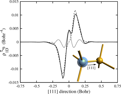
Figure 1: Electron-density response to an atomic displacement along the [111] direction in bulk Si (solid line). Its symmetric (dotted line) and antisymmetric (dashed line) parts are also plotted. The first-order density has been averaged in-plane. The origin of the abscissas coincides with the position of the atomic sublattice highlighted in the inset.

We first study bulk Si as a testcase. The quadrupolar tensor is defined by a single material constant, $Q$, via the following expression,

$$Q_{\kappa\beta}^{(2,\gamma\delta)}=(-1)^{\kappa+1}\,Q\,|\varepsilon_{\beta\gamma\delta}|,$$ (88)

$\varepsilon_{\beta\gamma\delta}$ is the Levi-Civita tensor. In order to benchmark the formalism, we first perform a calculation of $Q$ via an independent real-space method, which does not rely on Eq. (82). To this end, we calculate the charge-density response to an atomic displacement along $[111]$, by using a Brillouin-zone unfolding procedure Stengel (2016) applied to the 6-atoms hexagonal cell. In particular, we consider a stripe of 22 equidistant q-points (q=0 included), spanning the entire Brillouin zone along the crystallographic $[111]$ direction, and calculate the first-order densities associated with a phonon perturbation at each ${\bf q}$. (In practice, the number of independent ${\bf q}$-points reduces to 12 due to time-reversal symmetry.) After unfolding, we readily obtain the induced charge density that corresponds to a displacement of an isolated atom. (In practice, this approach corresponds to studying the displacement of a plane of atoms in a supercell where the hexagonal unit is repeated 22 times along [111].) We report the plane averages of the first-order density in Fig. 1, where we also show its decomposition into the antisymmetric and symmetric contributions. A fast decay of the induced density is clearly observed, which allows us to calculate the desired real-space moments with high numerical accuracy. The dipole moment correctly reproduces the pseudopotential charge, as expected. The second real-space moment of the first-order charge is then related to $Q$ via

$$Q^{\rm rs}=\frac{\sqrt{3}}{2}\epsilon_{\infty}\bar{Q}_{[111]}^{(2)},$$ (89)

where the superscript rs stands for “real space”, and $\epsilon_{\infty}$ is the calculated electronic dielectric constant.

Our calculated values are $\bar{Q}_{[111]}^{(2)}=1.178$ and $\epsilon_{\infty}=13.103$, which via Eq. (89) yield a value of $Q^{\rm{rs}}=13.367$ $\rm{e\cdot Bohr}$. With an equivalent choice of the computational parameters, by using our new method, Eq. (82) and the primitive 2-atom cell we obtain $Q=13.368$ $\rm{e\cdot Bohr}$. The matching between the two approaches is essentially perfect, which demonstrates the soundness of our implementation.

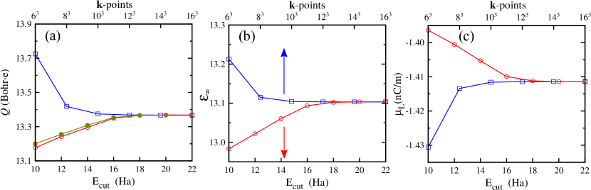
Figure 2: Convergence of selected linear-response quantities with respect to the plane-wave cutoff and the density of the ${\bf k}$-point mesh. Calculated dynamic quadrupole moment (a), dielectric constant (b) and longitudinal flexoelectric coefficient (c) are shown. Empty blue squares (lines are a guide to the eye) are obtained by varying the plane-waves energy cutoff while keeping the $12\times 12\times 12$ k-points grid fixed. Red empty circles correspond to varying the k-points mesh resolution with a fixed energy cut-off of 20 Ha. Panel (a) includes the energy cut-off dependence of the quadrupole constant as calculated from the second moment of the induced charge density response (green circles).

To better illustrate the plane-wave and ${\bf k}$-point mesh requirements of our new method, we have also performed a convergence study, where we compare the behavior of the quadrupole tensor components (alongside with the flexoelectric response, which we will comment on in Section V) to that of a “standard” linear-response quantity, the electronic dielectric constant. The numerical results are plotted in Fig. 2(a-b) as a function of the plane-waves energy cutoff and the number of k-points employed to sample the Brillouin zone. One can clearly appreciate from the figure that the quadrupoles (panel a) and the dielectric constant (panel b) converge equally fast with respect to both computational parameters. Moreover, the agreement between $Q$ and $Q^{\rm rs}$ becomes better and better as the energy cutoff is increased. Both observations concur to put our new method, based on Eq. (82), on very firm grounds. Note that the calculation via Eq. (82) is about an order of magnitude more efficient than the alternative real-space method, as the latter requires calculating the phonon response at many ${\bf q}$-points, while the former only requires $\Gamma$-point response functions as prerequisites.

	$\kappa=$Pb	$\kappa=$Ti	$\kappa=$O1	$\kappa=$O2	$\kappa=$O3
$Q_{\kappa 3}^{(2,11)}$	2.264	$-$3.545	2.884	$-$4.186	0.406
$Q_{\kappa 3}^{(2,22)}$	2.264	$-$3.545	$-$4.186	2.884	0.406
$Q_{\kappa 1}^{(2,31)}$	$-$0.062	$-$3.799	3.123	$-$1.115	$-$1.784
$Q_{\kappa 2}^{(2,32)}$	$-$0.062	$-$3.799	$-$1.115	3.123	$-$1.784
$Q_{\kappa 3}^{(2,33)}$	1.240	$-$0.195	2.027	2.027	6.653

Table 1: Quadrupole moments (in e$\cdot$Bohr) of PbTiO₃ calculated via Eq. (90). Note that $Q_{\kappa\alpha}^{(2,\beta\gamma)}=Q_{\kappa\alpha}^{(2,\gamma\beta)}$.

	$e_{113}=e_{223}$	$e_{311}=e_{322}$	$e_{333}$
Strain	0.1547	0.3617	$-$0.8345
Quadrupoles	0.1548	0.3614	$-$0.8347
Ref. Sàghi-Szabó et al.,1998	0.20	0.35	$-$0.88

Table 2: Clamped-ion piezoelectric coefficients (in C/m²) of PbTiO₃ calculated via two different methods. “Strain”: Standard DFPT approach, relying on the strain Hamann et al. (2005) and electric-field response. “Quadrupoles”: From the quadrupole moments via Eq. (90). Literature values from Ref. Sàghi-Szabó et al., 1998 are shown in italics for comparison.

Next, as a more ambitious test of our method, we carry out a numerical verification of Martin’s formula Martin (1972)

$$e_{\alpha\beta\gamma}=-\frac{1}{2\Omega}\sum_{\kappa}\left(Q_{\kappa\beta}^{(2,\alpha\gamma)}-Q_{\kappa\alpha}^{(2,\gamma\beta)}+Q_{\kappa\gamma}^{(2,\beta\alpha)}\right),$$ (90)

relating the proper Vanderbilt (2000) clamped-ion piezoelectric tensor $e_{\alpha\beta\gamma}$ to the sublattice sum of the dynamical quadrupoles. [Here, the first subscript ($\alpha$) of the piezoelectric tensor in the left-hand side indicates the polarization direction, whereas the other two indices ($\beta\gamma$) refer to the strain tensor components.] In particular, we shall benchmark the value of $e_{\alpha\beta\gamma}$ computed from Eq. (90) via the quadrupoles, against its value obtained as the mixed derivative of the energy with respect to components of the strain and the electric field. The latter is a standard DFPT quantity that we obtain by means of the metric tensor formulation by Hamann et al. Hamann et al. (2005) as implemented in the ABINIT package.

We focus on a well-known piezoelectric system, the tetragonal phase of PbTiO₃. The quadrupole moments of each atom in the unit cell are shown in Tab. 1. As for the three independent PbTiO₃ piezoelectric tensor elements, they are reported in Tab. 2. The comparison between the coefficients from the two methods demonstrates an exceptionally good agreement, which improves up to the fifth decimal digit by increasing the density of ${\bf k}$-points to $14\times 14\times 14$. Our results also qualitatively agree with those of Ref. Sàghi-Szabó et al., 1998, wherein a different set of lattice parameters, pseudopotentials and exchange-correlation functionals were employed.

V Flexoelectricity

V.1 Theory

From the point of view of atomistic calculations, flexoelectricity can be decomposed into three distinct contributions: Stengel (2013a) lattice-mediated, mixed and electronic. In principle, all three can be written, by using the formalism developed in this work, in terms of few basic ingredients. These are the mixed response to an electric field, atomic displacement or metric-wave perturbation taken at first or second order in ${\bf q}$. We defer the detailed implementation and test of the full flexoelectric tensor to a forthcoming publication, and focus here on the purely electronic response only.

The electronic flexoelectric tensor can be written as the second derivative with respect to ${\bf q}$ of the current-density that is adiabatically induced by a “clamped-ion” acoustic phonon perturbation, Dreyer et al. (2018) i.e. to a displacement pattern of the type

$${\bf R}_{l\kappa}={\bf R}_{l\kappa}^{0}+{\bf u}e^{i{\bf q\cdot}{\bf R}_{l\kappa}^{0}}.$$ (91)

Note the absence of the basis index on the perturbation parameter; this implies that all atoms in the primitive cell should be displaced simultaneously with equal amplitude, ${\bf u}$. Thus, a calculation of the flexoelectric tensor can be, in principle, carried out by regarding Eq. (91) as the sublattice sum of Eq. (78), which leads to the following practical scheme. First, one writes the polarization response to the displacement of an individual sublattice at finite ${\bf q}$; then, a second-order expansion in the wavevector ${\bf q}$ is performed; finally, the clamped-ion flexoelectric tensor is written as a sublattice sum of the result Stengel (2013a). This was indeed the strategy adopted in Ref. Dreyer et al., 2018.

In the context of this work, however, such an approach is impractical – the phonon perturbation of Eq. (78) does not vanish in the ${\bf q=0}$ limit. Therefore, Eq. (37) cannot be directly applied to calculate expansion to second order in ${\bf q}$ of the corresponding polarization response. To work around this obstacle, we shall follow Refs. Schiaffino et al., 2018; Stengel and Vanderbilt, 2018 and recast the acoustic phonon as a “metric wave” perturbation by operating a coordinate transformation to the curvilinear co-moving frame. We shall then write the polarization response to the acoustic phonon at finite ${\bf q}$ as (following the notation of Ref. Schiaffino et al., 2018)

$$\overline{P}_{\alpha,\beta}^{{}^{\prime}\bf q}=-\frac{2}{\Omega}E_{\bf q}^{\mathcal{E}_{\alpha}^{*}(\beta)},$$ (92)

where $E_{\bf q}^{\mathcal{E}_{\alpha}^{*}(\beta)}$ refers to the mixed derivative of Eq. (63) specialized to the case $\lambda=(\beta)$, and $(\beta)$ indicates a metric wave with the displacement field oriented along the Cartesian direction $\beta$. (The overline implies cell averaging, and the prime indicates that we have implicitly discarded the magnetic-like contribution from rotation gradients, following the arguments of Refs. Schiaffino et al., 2018; Stengel and Vanderbilt, 2018; Dreyer et al., 2018.)

It is useful, at this stage, to recall Schiaffino et al. (2018) two crucial properties of the metric wave: (i) both the perturbation and the response vanish at ${\bf q=0}$,

$$\hat{H}^{(\beta)}_{\bf k,q=0}=0,\qquad|u^{(\beta)}_{m\bf k,q=0}\rangle=0;$$ (93)

(ii) at first-order in ${\bf q}$, the metric wave reduces to the uniform strain perturbation, $\eta_{\beta\gamma}$, by Hamann et al. Hamann et al. (2005),

$$\hat{H}_{{\bf k},\delta}^{(\beta)}=i\hat{H}_{{\bf k}}^{\eta_{\beta\delta}},\qquad|u_{m{\bf k},\delta}^{(\beta)}\rangle=i|u_{m{\bf k}}^{\eta_{\beta\delta}}\rangle.$$ (94)

As we shall see shortly, properties (i) and (ii) will allow us to write down a closed expression for the clamped-ion flexoelectric tensor by using the second-order formula, Eq. (37). Before doing that, it is useful to perform a consistency check of Eq. (92) by showing that it correctly recovers the piezoelectric tensor at first order in ${\bf q}$ The clamped-ion piezoelectric tensor can be defined as

$$e_{\alpha\beta\gamma}=-i\frac{d}{dq_{\gamma}}\left(\frac{dP_{\alpha}^{\bf q}}{du_{\beta}}\right)\Big{|}_{\bf q=0}=i\frac{2}{\Omega}E_{\gamma}^{\mathcal{E}_{\alpha}^{*}(\beta)}.$$ (95)

By applying Hellmann-Feynman theorem to Eq. (63) and by using Eq. (93) and Eq. (94) we readily obtain

$$e_{\alpha\beta\gamma} = i\frac{2s}{\Omega}\int_{\rm BZ}[d^{3}k]\,\sum_{m}\langle u^{\mathcal{E}_{\alpha}}_{m{\bf k}}|\hat{H}^{(\beta)}_{\bf k,\gamma}|u^{(0)}_{m{\bf k}}\rangle$$ (96)

$$= -\frac{2s}{\Omega}\int_{\rm BZ}[d^{3}k]\,\sum_{m}\langle u^{\mathcal{E}_{\alpha}}_{m{\bf k}}|\hat{H}_{{\bf k}}^{\eta_{\beta\gamma}}|u^{(0)}_{m{\bf k}}\rangle,$$

which matches the established result. Gonze and Lee (1997); Hamann et al. (2005)

The type-I clamped-ion flexoelectric tensor can now be written in terms of the following formula,

$$\mu^{\rm I}_{\alpha\beta,\gamma\delta}=\frac{1}{\Omega}E^{\mathcal{E}_{\alpha}^{*}(\beta)}_{\gamma\delta},$$ (97)

where the mixed derivative is, as above, taken with respect to an electric field and the metric-wave perturbation. By taking again into account the relationships existing between the metric $(\beta)$ and the strain perturbations $\eta_{\beta\delta}$, the formulas for the second gradient , Eq. (37) and Eq. (38), are as follow,

$$\begin{split}&\widetilde{E}^{\mathcal{E}^{*}_{\alpha}\,(\beta)}_{\gamma\delta}=s\int_{\rm BZ}[d^{3}k]\sum_{m}\widetilde{E}^{\mathcal{E}^{*}_{\alpha}\,(\beta)}_{m{\bf k},\gamma\delta}\\ &\quad+\underbrace{\frac{i}{2}\int_{\Omega}\int K_{\gamma}({\bf r},{\bf r}^{\prime})n^{\mathcal{E}_{\alpha}}({\bf r})n^{\eta_{\beta\delta}}({\bf r}^{\prime})d^{3}rd^{3}r^{\prime}}_{T_{\rm elst}},\end{split}$$ (98)

$$\begin{split}&\widetilde{E}^{\mathcal{E}^{*}_{\alpha}\,(\beta)}_{m{\bf k},\gamma\delta}=\underbrace{i\langle u_{m{\bf k}}^{\mathcal{E}_{\alpha}}|\partial_{\gamma}\hat{H}^{(0)}_{{\bf k}}|u_{m{\bf k}}^{\eta_{\beta\delta}}\rangle}_{T_{1}}\\ &\quad+\underbrace{i\langle u_{m{\bf k}}^{\mathcal{E}_{\alpha}}|\partial_{\gamma}\hat{Q}_{{\bf k}}\hat{\mathcal{H}}_{{\bf k}}^{\eta_{\beta\delta}}|u_{m{\bf k}}^{(0)}\rangle}_{T_{2}}+\underbrace{i\langle u_{m{\bf k}}^{(0)}|\hat{V}^{\mathcal{E}_{\alpha}}\partial_{\gamma}\hat{Q}_{{\bf k}}|u_{m{\bf k}}^{\eta_{\beta\delta}}\rangle}_{T_{3}}\\ &\quad+\underbrace{\frac{1}{2}\langle u_{m{\bf k}}^{\mathcal{E}_{\alpha}}|\hat{H}_{{\bf k},\gamma\delta}^{(\beta)}|u_{m{\bf k}}^{(0)}\rangle}_{T_{4}}+\underbrace{i\langle i\,u_{m{\bf k},\gamma}^{A_{\alpha}}|u_{m{\bf k}}^{\eta_{\beta\delta}}\rangle}_{T_{5}}.\end{split}$$ (99)

Here we have labeled, for later reference, the five different terms of the band- and ${\bf k}$-resolved contribution as $T_{1-5}$, and the term deriving from the self-consistent energy via the gradient of the Coulomb kernel as $T_{\rm elst}$. Most of the symbols are self-explanatory, as we have already encountered them in the formula for the quadrupolar response. Similarly to the quadrupole case, we shall use Eq. (86) to simplify $T_{5}$; this is justified here because all our tests are performed on cubic materials, where $T_{5}$ must be symmetric with respect to $\alpha\gamma$. The formulas for the ${\bf q}$-derivatives of metric perturbation, $\hat{H}_{{\bf k},\gamma\delta}^{(\beta)}$, are elaborated in Appendix  B.2.

In the following subsection, we shall present our numerical results in type-II form by using

$$\mu^{\rm II}_{\alpha\gamma,\beta\delta}=\mu^{\rm I}_{\alpha\beta,\gamma\delta}+\mu^{\rm I}_{\alpha\delta,\beta\gamma}-\mu^{\rm I}_{\alpha\gamma,\delta\beta}.$$ (100)

In practice, the transformation Eq. (100) needs to be performed explicitly only on $T_{4}$, since all the other terms are most naturally written in type-II form. (The explicit formula is reported in Appendix B.2.) As we shall be dealing with cubic crystals only, we shall adopt the short-hand notation $\mu_{\rm L}=\mu^{\rm II}_{11,11}$, $\mu_{\rm T}=\mu^{\rm II}_{11,22}$ and $\mu_{\rm S}=\mu^{\rm II}_{12,12}$ for the three independent components, respectively: longitudinal (L), transverse (T) and shear(S). We shall drop the “II” superscript and assume that the flexoelectric tensor is in type-II form henceforth.

V.2 Computational parameters

The computation of the clamped-ion flexoelectric tensor has also been implemented in the ABINIT Gonze et al. (2009) package. The numerical results have been obtained with the same type of pseudopotentials and XC functional as in the Section IV.2. For our calculations on noble gas atoms He, Ar and Kr, we use a large cell of $14\times 14\times 14$ a.u., with a plane-wave cut-off of 90 Ha and a $2\times 2\times 2$ ($4\times 4\times 4$) mesh of ${\bf k}$-points to sample the Brillouin zone of He and Ar (of Kr). For our calculations on SrTiO₃, we used a cubic 5-atoms unit cell with an optimized cell parameter of $a_{0}$=7.267 Bohr, with a plane-wave cut-off of 70 Ha and a $8\times 8\times 8$ mesh of ${\bf k}$-points. Regarding Si, we use the 2-atom primitive cell with the same computational parameters as described in the Section IV.2. We have also performed a convergence study of the calculated Si flexoelectric tensor by varying the cut-off and ${\bf k}$-point mesh resolution.

V.3 Numerical results

	$\mu_{\rm L}$	$\mu_{\rm T}$	$\mu_{\rm S}\,(\times 10^{-4})$
He	$-$0.479 ($-$0.479a)	$-$0.479 ($-$0.479a)	$-$0.08 ($-$0.08a)
Ar	$-$4.821 ($-$4.813a)	$-$4.823 ($-$4.820a)	$-$1     ($-$10a)
Kr	$-$6.471 ($-$6.474a)	$-$6.477 ($-$6.476a)	$-$4     ($-$20a)

Table 3: Flexoelectric coefficients (in pC/m) of noble-gas atom systems. ^a Reference Schiaffino et al., 2018.

In order to test our method, we first study a simple cubic crystal lattice consisting of isolated noble-gas atoms, as already investigated in Refs.Stengel, 2013b; Stengel and Vanderbilt, 2016, 2018; Dreyer et al., 2018; Schiaffino et al., 2018. This toy model presents the advantage that its flexoelectric coefficients can be determined analytically, based on the macroscopic electric tensor and the second real-space moment of the unperturbed atomic charge. In particular, the three independent flexoelectric coefficients as calculated from a metric-wave perturbation, must fulfill the conditions Schiaffino et al. (2018); Stengel and Vanderbilt (2018)

$$\mu_{\rm L}=\mu_{\rm T},\qquad\mu_{\rm S}=0.$$ (101)

	$T_{\rm elst}$	$T_{1}$	$T_{2}$	$T_{3}$	$T_{4}$	$T_{5}$
$\mu_{\rm L}$	$-$6.472	3.512	$-$0.257	1.909	$-$9.367	5.854
$\mu_{\rm T}$	$-$1.885	$-$2.286	$-$0.257	0.000	$-$0.395	0.000
$\mu_{\rm S}$	$-$1.885	2.907	0.000	0.954	$-$4.903	2.926

Table 4: Contribution to the Ar flexoelectric coefficients (in pC/m) from the different terms of Eqs. (98) and (99).

Tab. 3 shows the flexoelectric coefficients calculated for He, Ar and Kr. It is clear from the reported data that the expected relationships, Eq. (101), are satisfied to a high degree of accuracy, and our coefficients are in excellent agreement with those obtained in previous works. Schiaffino et al. (2018) The largest deviation is shown by Kr: being it a larger atom, the overlap between neighboring images is likely to be more pronounced than in the other cases, which justifies the discrepancies we observe with respect to the expectations of the isolated atom model.

At this stage, it is worth emphasizing that such test is by no means trivial; on the contrary, it represents a very stringent benchmark for our formalism. To demonstrate this point, in Tab. 4 we show a breakdown of the three independent coefficients of the Ar-based crystal into the contributions of the individual terms appearing in Eqs. (98) and (99). The data in the table show a much more complex behavior than the final results of Tab. 3 would suggest. In particular, the conditions $\mu_{\rm L}=\mu_{\rm T}$ and $\mu_{\rm S}=0$ are not fulfilled by any of the individual terms (an exception is $T_{2}$, but it only contributes a tiny fraction of the final value); instead, the cancellation of the shear component and the equality between the transverse and longitudinal ones both result from a subtle balance between all the terms. Since each term involves a different combination of the input response functions and of the perturbations, such an accurate compensation clearly demonstrates the robustness of the numerical implementation.

	$\mu_{\rm L}$	$\mu_{\rm T}$	$\mu_{\rm S}$
Si (this work)	$-$1.4114	$-$1.0491	$-$0.1895
Ref.Schiaffino et al.,2018	$-$1.4110	$-$1.0493	$-$0.1894
SrTiO3 (this work)	$-$0.8848	$-$0.8262	$-$0.0823
Ref.Schiaffino et al.,2018	$-$0.8851	$-$0.8260	$-$0.0823
Ref.Stengel,2014	$-$0.883	$-$0.825	$-$0.082

Table 5: Flexoelectric coefficients (in nC/m) of Si and SrTiO₃ along with previous values found in the literature.

We have also calculated the electronic contribution to the flexoelectric tensor of two real materials, Si and SrTiO₃. The converged values of the flexoelectric coefficients are shown in Tab. 5, where we also compare them to the relevant literature data Schiaffino et al. (2018); Stengel (2014); Dreyer et al. (2018). Again, the excellent agreement with the published values is clear. Nevertheless, we stress that our results are obtained with a small fraction of the computational effort that was formerly needed.

As a final benchmark, we study the convergence of the flexoelectric coefficients of Si as a function of the ${\bf k}$-point mesh resolution and of the plane-wave cutoff. The results for $\mu_{\rm L}$ are shown in Fig. 2(c). (The convergence of the two other independent components is qualitatively similar to the longitudinal one.) Analogously to the case of the quadrupoles, the flexoelectric coefficients converge at the same rate as the dielectric tensor. This means that all the spatial dispersion properties that we have calculated in this work require a computational effort that is comparable to the study of other standard linear-response quantities, such as the electronic dielectric tensor.

VI Conclusions and outlook

We have established a general method to perform a systematic study of spatial dispersion effects in the framework of density-functional perturbation theory. As a practical demonstration, we have implemented the dynamical quadrupole tensor and the clamped-ion flexoelectric tensor in the ABINIT package, and performed extensive numerical tests. This work opens a number of exciting avenues for future research, which we shall briefly sketch hereafter.

First, we expect that the knowledge of the dynamical quadrupoles will allow for an improved description of the interatomic force constants, thereby enabling a more accurate computation of the phonon band structures. This might be important for certain material classes, such as piezoelectrics, where the treatment of long-range electrostatics is crucial for reproducing the correct sound velocity. Wu et al. (2005) On a different note, our theory might also prove itself very helpful in establishing higher-order multipolar generalizations Benalcazar et al. (2017) of the Berry-phase theory of polarization King-Smith and Vanderbilt (1993). Indeed, our expressions for the dynamical quadrupole and flexoelectric tensors can be regarded as the linear variation of the “bulk quadrupolization” Wheeler et al. (2018) with respect to a zone-center lattice distortion or uniform strain, respectively. There are intriguing parallels to the theory of multipolar magnetic orders Ederer and Spaldin (2007); Spaldin et al. (2013) as well, which will certanly stimulate further studies.

Second, the treatment of flexoelectric effects beyond the clamped-ion level should be relatively straightforward by following the same guidelines as we did here. Both the “mixed” and “lattice-mediated” contributions involve first or second derivatives of the polarization response to a phonon, or the force-constant matrix, just like the electronic contribution. These additional pieces involve similar formulas, only with a slightly different combination of the basic response functions (electric field, atomic displacement or uniform strain). Thus, the calculation of the full flexoelectric tensor for an insulating crystal or nanostructure of arbitrary symmetry looks now well within reach. We expect that, once implemented, it will involve a computational effort that is comparable to the calculation of the piezoelectric tensor.

Third, the method can be easily adapted to compute other spatial dispersion effects, for example the natural optical rotation tensor. (The latter can be written as the first gradient with respect to the wavevector of the dielectric tensor.) First-principles calculations of natural gyrotropy are starting to appear; Tsirkin et al. (2018) we expect that, by bringing it within the scopes of DFPT, the formalism presented here will greatly simplify the calculation of this interesting quantity as well. In the context of ferroic materials, we also expect our method to facilitate the development of first-principles based continuum models Schiaffino and Stengel (2017) and effective Hamiltonians Zhong et al. (1994), where gradient-mediated couplings often play an important role.

More generally, our work has revealed a profound connection between spatial dispersion and orbital magnetism that, in our opinion, deserves further attention. Whenever the polarization response to a perturbation is needed at first order in the wavevector ${\bf q}$, one of the contributions necessarily involves the wave-function response to a gradient of ${\bf A}$, and hence to a uniform magnetic field. This can be tentatively interpreted as a “gyrotropic” contribution to the response, and is only present in certain crystal classes; we were unable to discuss it here because of space limitations, but we regard it as yet another interesting topic for future studies.

Appendix A Response to the electromagnetic vector potential in the long-wavelength limit

The functions $|u^{A_{\alpha}}_{m{\bf k,\gamma}}\rangle$ are the ${\bf q}$-derivatives of the functions $|u^{A_{\alpha}}_{m{\bf k,q}}\rangle$, which are defined as the solutions of the Sternheimer equation, Eq. (55). In the following, we shall proceed to explicitly demonstrate Eq. (57), by performing the formal expansion of Eq. (55) to first order in ${\bf q}$.

By deriving both sides of the Sternheimer equation with respect to $q_{\gamma}$, one obtains

$$\left(\hat{H}^{(0)}_{\bf k}+a\hat{P}_{\bf k}-\epsilon^{(0)}_{n{\bf k}}\right)|u^{A_{\alpha}}_{n{\bf k},\gamma}\rangle = -\left(\partial_{\gamma}\hat{H}^{(0)}_{\bf k}+a\partial_{\gamma}\hat{P}_{\bf k}\right)|u^{A_{\alpha}}_{n{\bf k}}\rangle-\partial_{\gamma}\hat{Q}_{\bf k}\,\partial_{\alpha}\hat{H}^{(0)}_{\bf k}\,|u^{(0)}_{n{\bf k}}\rangle-\frac{1}{2}\hat{Q}_{\bf k}\,\partial^{2}_{\alpha\gamma}\hat{H}^{(0)}_{\bf k}\,|u^{(0)}_{n{\bf k}}\rangle.$$ (102)

(We shall drop the superscript “(0)” on the ground-state Hamiltonian operator from now on, to simplify the notation.) One can now use the zero-th order result, Eq. (56), to achieve the following expression (I shall also use $\partial_{\alpha}\hat{Q}_{\bf k}=-\partial_{\alpha}\hat{P}_{\bf k}$ whenever appropriate),

$$\left(\hat{H}_{\bf k}+a\hat{P}_{\bf k}-\epsilon_{n{\bf k}}\right)|u^{A_{\alpha}}_{n{\bf k},\gamma}\rangle = \Big{(}\partial_{\gamma}\hat{H}_{\bf k}\,\partial_{\alpha}\hat{Q}_{\bf k}-a\partial_{\gamma}\hat{P}_{\bf k}\,\partial_{\alpha}\hat{P}_{\bf k}-\partial_{\gamma}\hat{Q}_{\bf k}\,\partial_{\alpha}\hat{H}_{\bf k}\,-\frac{1}{2}\hat{Q}_{\bf k}\,\partial_{\alpha}\partial_{\gamma}\hat{H}_{\bf k}\Big{)}|u^{(0)}_{n{\bf k}}\rangle.$$ (103)

It is convenient, at this point, to separately treat the contributions that are symmetric and antisymmetric under $\alpha\gamma$ exchange.

A.1 Symmetric part

We have

$$\left(\hat{H}_{\bf k}+a\hat{P}_{\bf k}-\epsilon_{n{\bf k}}\right)\left(|u^{A_{\alpha}}_{n{\bf k},\gamma}\rangle+|u^{A_{\gamma}}_{n{\bf k},\alpha}\rangle\right) = \Big{(}-a\partial_{\gamma}\hat{P}_{\bf k}\,\partial_{\alpha}\hat{P}_{\bf k}-a\partial_{\alpha}\hat{P}_{\bf k}\,\partial_{\gamma}\hat{P}_{\bf k}+\partial_{\gamma}\hat{H}_{\bf k}\,\partial_{\alpha}\hat{Q}_{\bf k}+\partial_{\alpha}\hat{H}_{\bf k}\,\partial_{\gamma}\hat{Q}_{\bf k}$$ (104)

$$\quad-\partial_{\gamma}\hat{Q}_{\bf k}\,\partial_{\alpha}\hat{H}_{\bf k}-\partial_{\alpha}\hat{Q}_{\bf k}\,\partial_{\gamma}\hat{H}_{\bf k}-\hat{Q}_{\bf k}\,\partial_{\alpha}\partial_{\gamma}\hat{H}_{\bf k}\Big{)}|u^{(0)}_{n{\bf k}}\rangle.$$

The long parenthesis on the right-hand side contains a total of seven terms. The third to the seventh can be rewritten more compactly by observing that $\partial^{2}_{\alpha\gamma}\left[\hat{Q}_{\bf k},\hat{H}_{\bf k}\right]=0$, leading to

$$\left(\hat{H}_{\bf k}+a\hat{P}_{\bf k}-\epsilon_{n{\bf k}}\right)\left(|u^{A_{\alpha}}_{n{\bf k},\gamma}\rangle+|u^{A_{\gamma}}_{n{\bf k},\alpha}\rangle\right)=\Big{(}-a\partial_{\gamma}\hat{P}_{\bf k}\,\partial_{\alpha}\hat{P}_{\bf k}-a\partial_{\alpha}\hat{P}_{\bf k}\,\partial_{\gamma}\hat{P}_{\bf k}-\left[\hat{H}_{\bf k},\partial^{2}_{\alpha\gamma}\hat{Q}_{\bf k}\right]\Big{)}|u^{(0)}_{n{\bf k}}\rangle.$$ (105)

The solution is given by

$$|u^{A_{\alpha}}_{n{\bf k},\gamma}\rangle+|u^{A_{\gamma}}_{n{\bf k},\alpha}\rangle=-\partial^{2}_{\alpha\gamma}\hat{Q}_{\bf k}|u^{(0)}_{n{\bf k}}\rangle=\partial^{2}_{\alpha\gamma}\hat{P}_{\bf k}|u^{(0)}_{n{\bf k}}\rangle.$$ (106)

To justify the above derivation, observe that

$$\partial^{2}_{\alpha\gamma}(PP)=\partial_{\alpha}P\partial_{\gamma}P+\partial_{\gamma}P\partial_{\alpha}P+\partial^{2}_{\alpha\gamma}PP+P\partial^{2}_{\alpha\gamma}P.$$

Using the idempotency of $P$, this immediately leads to

$$P\,\partial^{2}_{\alpha\gamma}P\,P=-P\left(\partial_{\gamma}P\,\partial_{\alpha}P+\partial_{\alpha}P\,\partial_{\gamma}P\right)P.$$

Note that the response is purely “geometric”, i.e. only given in terms of the ground-state wavefunctions. In spite of that, the response contains both valence and conduction-band components, as the operator $\partial^{2}_{\alpha\gamma}\hat{P}_{\bf k}$ generally has both inner and cross-gap matrix elements.

A.2 Antisymmetric part

The antisymmetric part can be written as follows,

$$\left(\hat{H}_{\bf k}+a\hat{P}_{\bf k}-\epsilon_{n{\bf k}}\right)\left(|u^{A_{\alpha}}_{n{\bf k},\gamma}\rangle-|u^{A_{\gamma}}_{n{\bf k},\alpha}\rangle\right) = \Big{(}-a\partial_{\gamma}\hat{P}_{\bf k}\,\partial_{\alpha}\hat{P}_{\bf k}+a\partial_{\alpha}\hat{P}_{\bf k}\,\partial_{\gamma}\hat{P}_{\bf k}+\partial_{\gamma}\hat{H}_{\bf k}\,\partial_{\alpha}\hat{Q}_{\bf k}$$ (107)

$$\quad-\partial_{\alpha}\hat{H}_{\bf k}\,\partial_{\gamma}\hat{Q}_{\bf k}-\partial_{\gamma}\hat{Q}_{\bf k}\,\partial_{\alpha}\hat{H}_{\bf k}+\partial_{\alpha}\hat{Q}_{\bf k}\,\partial_{\gamma}\hat{H}_{\bf k}\Big{)}|u^{(0)}_{n{\bf k}}\rangle.$$

This can be expressed more compactly by using (anti)commutators,

$$\left(\hat{H}_{\bf k}+a\hat{P}_{\bf k}-\epsilon_{n{\bf k}}\right)\left(|u^{A_{\alpha}}_{n{\bf k},\gamma}\rangle-|u^{A_{\gamma}}_{n{\bf k},\alpha}\rangle\right) = \Big{(}-a[\partial_{\gamma}\hat{P}_{\bf k},\partial_{\alpha}\hat{P}_{\bf k}]-\left\{\partial_{\gamma}\hat{H}_{\bf k},\partial_{\alpha}\hat{P}_{\bf k}\right\}+\left\{\partial_{\alpha}\hat{H}_{\bf k},\partial_{\gamma}\hat{P}_{\bf k}\right\}\Big{)}|u^{(0)}_{n{\bf k}}\rangle.$$ (108)

To recast the above equation into a more transparent form, it is useful to work out the following expression,

$$\left[H,\partial_{\gamma}P\partial_{\alpha}P-\partial_{\alpha}P\partial_{\gamma}P\right] = \left[H,\partial_{\gamma}P\right]\partial_{\alpha}P-\left[H,\partial_{\alpha}P\right]\partial_{\gamma}P-\partial_{\gamma}P\left[\partial_{\alpha}P,H\right]+\partial_{\alpha}P\left[\partial_{\gamma}P,H\right]$$ (109)

$$= -\left[\partial_{\gamma}H,P\right]\partial_{\alpha}P+\left[\partial_{\alpha}H,P\right]\partial_{\gamma}P+\partial_{\gamma}P\left[P,\partial_{\alpha}H\right]-\partial_{\alpha}P\left[P,\partial_{\gamma}H\right]$$

$$= P\partial_{\gamma}H\partial_{\alpha}P-P\partial_{\alpha}H\partial_{\gamma}P-P\partial_{\gamma}P\partial_{\alpha}H+P\partial_{\alpha}P\partial_{\gamma}H$$

$$= P\left\{\partial_{\gamma}H,\partial_{\alpha}P\right\}-P\left\{\partial_{\alpha}H,\partial_{\gamma}P\right\},$$

where the fact that the expression must be applied to a valence ket has been used to go from the third to the fourth line. The Sternheimer equation can then be rewritten as

$$\left(\hat{H}_{\bf k}+a\hat{P}_{\bf k}-\epsilon_{n{\bf k}}\right)\left(|u^{A_{\alpha}}_{n{\bf k},\gamma}\rangle-|u^{A_{\gamma}}_{n{\bf k},\alpha}\rangle\right) = -\left(\hat{H}_{\bf k}+a\hat{P}_{\bf k}-\epsilon_{n{\bf k}}\right)\left[\partial_{\gamma}\hat{P}_{\bf k},\partial_{\alpha}\hat{P}_{\bf k}\right]|u^{(0)}_{n{\bf k}}\rangle$$

$$-\hat{Q}_{\bf k}\left(\left\{\partial_{\gamma}\hat{H}_{\bf k},\partial_{\alpha}\hat{P}_{\bf k}\right\}+\left\{\partial_{\alpha}\hat{H}_{\bf k},\partial_{\gamma}\hat{P}_{\bf k}\right\}\right)|u^{(0)}_{n{\bf k}}\rangle.$$

and, finally,

$$\left(\hat{H}_{\bf k}+a\hat{P}_{\bf k}-\epsilon_{n{\bf k}}\right)|u^{\rm CG}_{n{\bf k},\gamma}\rangle=-\hat{Q}_{\bf k}\left(\left\{\partial_{\gamma}\hat{H}_{\bf k},\partial_{\alpha}\hat{P}_{\bf k}\right\}-\left\{\partial_{\alpha}\hat{H}_{\bf k},\partial_{\gamma}\hat{P}_{\bf k}\right\}\right)|u^{(0)}_{n{\bf k}}\rangle,$$ (110)

where we have defined

$$|u^{\rm CG}_{n{\bf k},\gamma}\rangle=|u^{A_{\alpha}}_{n{\bf k},\gamma}\rangle-|u^{A_{\gamma}}_{n{\bf k},\alpha}\rangle+\left[\partial_{\gamma}\hat{P}_{\bf k},\partial_{\alpha}\hat{P}_{\bf k}\right]|u^{(0)}_{n{\bf k}}\rangle.$$ (111)

By combining Eq. (106) and Eq. (111) we recover Eq. (57).

Appendix B ${\bf q}$-derivatives of first order Hamiltonians

B.1 First ${\bf q}$-derivative of atomic displacement Hamiltonian

The first-order Hamiltonian with respect to an atomic displacement consists of a local potential plus a nonlocal separable contribution,

$$V_{\bf q}^{{\rm loc},\tau_{\kappa\beta}}({\bf G}) = -i(G_{\beta}+q_{\beta})\frac{1}{\Omega}e^{-i{\bf G}\cdot\bm{\tau}_{\kappa}}\,v^{\rm loc}_{\kappa}({\bf G+q}),$$ (112)

$$V^{{\rm sep},\tau_{\kappa\beta}}_{\bf k,q}({\bf G},{\bf G}^{\prime}) = -i(G_{\beta}+q_{\beta}-G^{\prime}_{\beta})\frac{1}{\Omega}\sum_{\mu}e^{-i({\bf G-G^{\prime}})\cdot\bm{\tau}_{\kappa}}\,e_{\mu\kappa}\zeta_{\mu\kappa}({\bf k+q+G})\zeta^{*}_{\mu\kappa}({\bf k+G}^{\prime}).$$ (113)

Note that the above formulas slightly differ from the standard implementations of DFPT. Gonze (1997) This is because in formulating them we have used a different convention Stengel (2013a) for the sublattice-dependent phase factors. Such difference is rooted in our assumption of a displacement pattern of the type $e^{i\bf{q}\bf{R}_{l\kappa}}$, instead of the typical one ($e^{i\bf{q}\bf{R}_{l}}$). This leads to a much simpler and physically transparent treatment of the long-wave expansion. At ${\bf q}$=0, the present theory reduces to the standard treatment.

By differentiating the above formulas, we arrive at the following expressions for the first ${\bf q}$-gradients (at ${\bf q}$=0) of the perturbation, which are necessary for the dynamical quadrupoles calculation,

$$V_{\gamma}^{{\rm loc},\tau_{\kappa\beta}}({\bf G}) = -i\frac{1}{\Omega}e^{-i{\bf G}\bm{\tau}_{\kappa}}\Big{(}\delta_{\beta\gamma}\,v_{\kappa}^{\rm loc}(G)+\frac{G_{\beta}G_{\gamma}}{G}\,v_{\kappa}^{\rm loc}(G)^{\prime}\Big{)},$$ (114)

$$V_{{\bf k},\gamma}^{{\rm sep},\tau_{\kappa\beta}}({\bf G},{\bf G}^{\prime}) = -i\frac{1}{\Omega}\sum_{\mu}e^{-i({\bf G}-{\bf G}^{\prime})\bm{\tau}_{\kappa}}e_{\mu\kappa}\Big{(}\delta_{\beta\gamma}\,\zeta_{\mu\kappa}({\bf k}+{\bf G})\zeta_{\mu\kappa}^{*}({\bf k}+{\bf G}^{\prime})\,+$$ (115)

$$\qquad\qquad(G_{\beta}-G_{\beta}^{\prime})\,\zeta_{\mu\kappa,\gamma}({\bf k}+{\bf G})\zeta_{\mu\kappa}^{*}({\bf k}+{\bf G}^{\prime})\Big{)},$$

where $G=|{\bf G}|$, $v_{\kappa}^{\rm loc}(G)^{\prime}$ is the first derivative of the spherical atomic pseudopotential, and $\zeta_{\mu\kappa,\gamma}({\bf k}+{\bf G})$ is the ${\bf q}$-derivative along the $\gamma$ direction of the separable nonlocal projector.

B.2 Second ${\bf q}$-derivative of metric perturbation Hamiltonian

The first-order Hamiltonian of the metric perturbation is Schiaffino et al. (2018)

$$\hat{H}^{(\beta)}_{\bf k,q}=\hat{T}^{(\beta)}_{\bf k,q}+\hat{V}_{\bf k,q}^{{\rm psp},(\beta)}+\hat{V}_{\bf q}^{{\rm H0},(\beta)}+\hat{V}_{\bf q}^{{\rm XC0},(\beta)}+\hat{V}_{\bf q}^{{\rm geom},(\beta)},$$ (116)

where the terms on the right-hand side correspond to the kinetic ($\hat{T}$), pseudopotential (psp), Hartree (H0), exchange-correlation (XC0) and geometric contributions to the external potential. The pseudopotential term, in turn, consists of a local plus a separable contribution,

$$V_{\bf k,q}^{{\rm psp},(\beta)}({\bf G,G}^{\prime})=V_{\bf q}^{{\rm loc},(\beta)}({\bf G-G}^{\prime})+V_{\bf k,q}^{{\rm sep},(\beta)}({\bf G,G}^{\prime})$$ (117)

The explicit formulas for each of these terms are reported in Ref. Schiaffino et al., 2018. In the following, we list the formulas for the second ${\bf q}$-gradients (at ${\bf q}=0$) of these contributions required in the calculation of the clamped-ion flexoelectric tensor (see, e.g., Eq. (99)).

The kinetic contribution:

$$\begin{split}T^{(\beta)}_{{\bf k},\gamma\delta}({\bf G},{\bf G}^{\prime})=-i\Big{(}\delta_{\gamma\delta}(k_{\beta}+G_{\beta})+\delta_{\beta\gamma}\frac{1}{2}(k_{\delta}+G_{\delta})+\delta_{\beta\delta}\frac{1}{2}(k_{\gamma}+G_{\gamma})\Big{)}\delta_{{\bf G}{\bf G}^{\prime}}.\end{split}$$ (118)

The local part of the pseudopotential:

$$\begin{split}V_{\gamma\delta}^{{\rm loc},\,(\beta)}({\bf G})=-i\frac{1}{\Omega}\sum_{\kappa}e^{-i{\bf G}\tau_{\kappa}}\Bigg{(}\frac{v_{\kappa}^{\rm loc}(G)^{\prime}}{G}\Big{(}\delta_{\beta\delta}G_{\gamma}+\delta_{\beta\gamma}G_{\delta}+\delta_{\gamma\delta}G_{\beta}-\frac{G_{\beta}G_{\delta}G_{\gamma}}{G^{2}}\Big{)}+\frac{v_{\kappa}^{\rm loc}(G)^{\prime\prime}}{G^{2}}G_{\beta}G_{\delta}G_{\gamma}\Bigg{)},\end{split}$$ (119)

with $v_{\kappa}^{\rm loc}(G)^{\prime\prime}$ being the second derivative of the spherical atomic pseudopotential

The separable part of the pseudopotential:

$$\begin{split}&V^{{\rm sep},(\beta)}_{{\bf k},\gamma\delta}=-\frac{i}{\Omega}\sum_{\mu\kappa}e_{\mu\kappa}\,e^{-i({\bf G}-{\bf G}^{\prime})\tau_{\kappa}}\Bigg{(}\Big{(}\frac{3}{2}\delta_{\beta\gamma}\,\zeta_{\mu\kappa,\delta}({\bf k}+{\bf G})+\frac{3}{2}\delta_{\beta\delta}\,\zeta_{\mu\kappa,\gamma}({\bf k}+{\bf G})+(k_{\beta}+G_{\beta})\zeta_{\mu\kappa,\delta\gamma}({\bf k}+{\bf G})\Big{)}\zeta^{*}_{\mu\kappa}({\bf k}+{\bf G}^{\prime})\\ &\quad+\frac{1}{2}\delta_{\beta\delta}\,\zeta_{\mu\kappa}({\bf k}+{\bf G})\zeta^{*}_{\mu\kappa,\gamma}({\bf k}+{\bf G}^{\prime})+\zeta_{\mu\kappa,\delta}({\bf k}+{\bf G})\zeta^{*}_{\mu\kappa,\gamma}({\bf k}+{\bf G}^{\prime})(k_{\beta}+G^{\prime}_{\beta})+\frac{1}{2}\delta_{\beta\gamma}\zeta_{\mu\kappa}({\bf k}+{\bf G})\zeta^{*}_{\mu\kappa,\delta}({\bf k}+{\bf G}^{\prime})\\ &\quad+\zeta_{\mu\kappa,\gamma}({\bf k}+{\bf G})\zeta^{*}_{\mu\kappa,\delta}({\bf k}+{\bf G}^{\prime})(k_{\beta}+G^{\prime}_{\beta})+\zeta_{\mu\kappa}({\bf k}+{\bf G})\zeta^{*}_{\mu\kappa,\delta\gamma}({\bf k}+{\bf G}^{\prime})(k_{\beta}+G^{\prime}_{\beta})\Bigg{)},\end{split}$$ (120)

with $\zeta_{\mu\kappa,\gamma\delta}({\bf k}+{\bf G})$ being the second ${\bf q}$-derivative along the $\gamma$ and $\delta$ direction of the separable nonlocal projector.

The remaining terms Schiaffino et al. (2018) include the XC and geometric contributions that vanish at second order in ${\bf q}$ and a Hartree contribution whose second ${\bf q}$-gradient is,

$$\begin{split}\hat{V}_{\delta\gamma}^{{\rm H0},(\beta)}({\bf G})=-i\,8\pi\frac{n^{(0)}({\bf G})}{G^{2}}\Big{(}\frac{4\,G_{\beta}\,G_{\delta}\,G_{\gamma}}{G^{4}}-\frac{\delta_{\beta\delta}G_{\gamma}+\delta_{\beta\gamma}G_{\delta}+\delta_{\delta\gamma}G_{\beta}}{G^{2}}\Big{)},\end{split}$$ (121)

where $n^{(0)}({\bf G})$ refers to the ground state electron density.

It is useful, at this point, to perform a further rearrangement of $\hat{H}_{{\bf k},\gamma\delta}^{(\beta)}$ by defining

$$\hat{H}_{{\bf k},\gamma}^{(\beta\delta)}=\hat{H}_{{\bf k},\gamma\delta}^{(\beta)}+\hat{H}_{{\bf k},\beta\gamma}^{(\delta)}-\hat{H}_{{\bf k},\beta\delta}^{(\gamma)}.$$ (122)

This allows us to write the flexoelectric tensor directly in type-II form as

$$\mu^{\rm II}_{\alpha\gamma,\beta\delta}=\frac{2}{\Omega}E^{\mathcal{E}_{\alpha}^{*}(\beta\delta)}_{\gamma},$$ (123)

where

$$\begin{split}&E^{\mathcal{E}^{*}_{\alpha}\,(\beta\delta)}_{\gamma}=s\int_{\rm BZ}[d^{3}k]\sum_{m}E^{\mathcal{E}^{*}_{\alpha}\,(\beta\delta)}_{m{\bf k},\gamma}+\underbrace{\frac{i}{2}\int_{\Omega}\int K_{\gamma}({\bf r},{\bf r}^{\prime})n^{\mathcal{E}_{\alpha}}({\bf r})n^{\eta_{\beta\delta}}({\bf r}^{\prime})d^{3}rd^{3}r^{\prime}}_{T_{\rm elst}},\end{split}$$ (124)

and

$$\begin{split}E^{\mathcal{E}^{*}_{\alpha}\,(\beta\delta)}_{m{\bf k},\gamma}=&\underbrace{i\langle u_{m{\bf k}}^{\mathcal{E}_{\alpha}}|\partial_{\gamma}\hat{H}^{(0)}_{{\bf k}}|u_{m{\bf k}}^{\eta_{\beta\delta}}\rangle}_{T_{1}}+\underbrace{i\langle u_{m{\bf k}}^{\mathcal{E}_{\alpha}}|\partial_{\gamma}\hat{Q}_{{\bf k}}\hat{\mathcal{H}}_{{\bf k}}^{\eta_{\beta\delta}}|u_{m{\bf k}}^{(0)}\rangle}_{T_{2}}+\underbrace{i\langle u_{m{\bf k}}^{(0)}|\hat{V}^{\mathcal{E}_{\alpha}}\partial_{\gamma}\hat{Q}_{{\bf k}}|u_{m{\bf k}}^{\eta_{\beta\delta}}\rangle}_{T_{3}}\\ &\quad+\underbrace{\frac{1}{2}\langle u_{m{\bf k}}^{\mathcal{E}_{\alpha}}|\hat{H}_{{\bf k},\gamma}^{(\beta\delta)}|u_{m{\bf k}}^{(0)}\rangle}_{T_{4}}+\underbrace{i\langle i\,u_{m{\bf k},\gamma}^{A_{\alpha}}|u_{m{\bf k}}^{\eta_{\beta\delta}}\rangle}_{T_{5}}.\end{split}$$ (125)

Appendix C Treatment of the electrostatic divergence at ${\bf G}=0$

The local potential diverges at ${\bf G}=0$ because of the Coulomb singularity, Gonze (1997)

$$v^{{\rm loc}}_{\kappa}(q)\sim-\frac{4\pi}{q^{2}}Z_{\kappa},$$ (126)

where $Z_{\kappa}$ is the bare pseudopotential charge. This means that the ${\bf q}$-derivatives of the local potential contribution to the first-order Hamiltonians discussed in the previous sections must be calculated with some care regarding the ${\bf G}=0$ component. To see this, it is useful to rewrite Eq. (126) as follows,

$$v^{{\rm loc}}_{\kappa}(q)=\frac{F_{\kappa}(q)}{q^{2}},$$ (127)

where we have introduced the auxiliary function

$$F_{\kappa}(q)\sim-4\pi Z_{\kappa}+\frac{q^{2}}{2}F_{\kappa}^{\prime\prime}.$$ (128)

Regarding the atomic displacement perturbation, the above definitions lead to the following small-${\bf q}$ expansion of the local potential part at ${\bf G}=0$,

$$V_{{\bf q}}^{\rm loc,\tau_{\kappa\beta}}({\bf G}=0)\sim-\frac{iq_{\beta}}{\Omega}\left(-\frac{4\pi Z_{\kappa}}{q^{2}}+\frac{F_{\kappa}^{\prime\prime}}{2}\right).$$ (129)

Because of the assumption of short-circuit electrical boundary conditions we shall drop the divergent term. This leaves us with a constant multiplied by $q_{\beta}$, which vanishes in the ${\bf q}\rightarrow 0$ limit. The ${\bf q}$-derivative does not vanish,

$$V_{\gamma}^{\rm loc,\tau_{\kappa\beta}}({\bf G}=0)\rightarrow-\frac{i}{2\Omega}F_{\kappa}^{\prime\prime}\delta_{\beta\gamma},$$ (130)

and we should in principle take it into account in the calculation of the quadrupolar tensor. However, in Eq. (85) the operator $\hat{H}_{\bf k\gamma}^{\tau_{\kappa\beta}}$ only appears between a conduction-band bra and a valence-band ket. By orthogonality, the above constant contribution is irrelevant and can be safely discarded.

Regarding the metric perturbation, recall that it vanishes in the ${\bf q}\rightarrow 0$ limit, as the aforementioned divergence in the local potential contribution exactly cancels with an opposite divergence in the “H0” term. Schiaffino et al. (2018) Within the present notation conventions, one has

$$\begin{split}&V_{{\bf q}}^{\rm loc+H0,(\beta)}({\bf G}=0)\\ &\quad=-\frac{i}{\Omega}\frac{q_{\beta}}{q^{2}}\big{(}\sum_{\kappa}F_{\kappa}(q)-4\pi\Omega n^{(0)}({\bf G}=0)\big{)}\\ &\quad=-\frac{i}{2\Omega}q_{\beta}\sum_{\kappa}F_{\kappa}^{\prime\prime}+O(q^{3}),\end{split}$$ (131)

where in the last line we have taken into account that $F_{\kappa}(q=0)=4\pi Z_{\kappa}$ Gonze (1997), that $n^{(0)}({\bf G}=0)=\frac{\sum_{\kappa}Z_{\kappa}}{\Omega}$ and that odd terms in the Taylor expansion of $F_{\kappa}(q)$ vanish due to the spherical symmetry of the local atomic potentials. The first ${\bf q}$-derivative of the above yields a well-defined constant,

$$V_{\gamma}^{\rm loc+H0,(\beta)}({\bf G}=0)=-\frac{i}{2\Omega}\delta_{\beta\gamma}\sum_{\kappa}F_{\kappa}^{\prime\prime}.$$ (132)

Recall that the first ${\bf q}$-derivative of the metric-wave perturbation coincides (modulo a factor of $i$) with the uniform strain perturbation. Hence, we conclude that to calculate the clamped-ion flexoelectric tensor the ${\bf G}=0$ component of the local potential of the first-order strain Hamiltonian has to be corrected as,

$$V^{{\rm loc},\eta_{\beta\delta}}({\bf G}=0)=V_{\delta}^{{\rm loc},(\beta)}({\bf G}=0)=-\frac{i}{2\Omega}\delta_{\beta\delta}\sum_{\kappa}F_{\kappa}(q)^{\prime\prime}.$$ (133)

This correction is important in the calculation of the flexoelectric tensor, since the uniform strain operator in Eq. (99) appears sandwiched between two unperturbed valence states.

References

- Malashevich and Souza (2010) Andrei Malashevich and Ivo Souza, “Band theory of spatial dispersion in magnetoelectrics,” Phys. Rev. B 82, 245118 (2010).
- Prosandeev et al. (2013) Sergey Prosandeev, Andrei Malashevich, Zhigang Gui, Lydie Louis, Raymond Walter, Ivo Souza, and L. Bellaiche, “Natural optical activity and its control by electric field in electrotoroidic systems,” Phys. Rev. B 87, 195111 (2013).
- Portigal and Burstein (1968) D. L. Portigal and E. Burstein, “Acoustical activity and other first-order spatial dispersion effects in crystals,” Phys. Rev. 170, 673–678 (1968).
- Tagantsev (1986) A. K. Tagantsev, “Piezoelectricity and flexoelectricity in crystalline dielectrics,” Phys. Rev. B 34, 5883 (1986).
- Zubko et al. (2013) P. Zubko, G. Catalan, and A. K. Tagantsev, “Flexoelectric effect in solids,” Annu. Rev. Mater. Res. 43, 387–421 (2013).
- Stengel and Vanderbilt (2016) Massimiliano Stengel and David Vanderbilt, “First-principles theory of flexoelectricity,” in Flexoelectricity in Solids From Theory to Applications, edited by Alexander K. Tagantsev and Petr V. Yudin (World Scientific Publishing Co., Singapore, 2016) Chap. 2, pp. 31–110.
- Bhaskar et al. (2016) Umesh Kumar Bhaskar, Nirupam Banerjee, Amir Abdollahi, Zhe Wang, Darrell G Schlom, Guus Rijnders, and Gustau Catalan, “A flexoelectric microelectromechanical system on silicon,” Nature nanotechnology 11, 263–266 (2016).
- Lu et al. (2012) H. Lu, C.-W. Bark, D. Esque de los Ojos, J. Alcala, C. B. Eom, G. Catalan, and A. Gruverman, “Mechanical writing of ferroelectric polarization,” Science 336, 59–61 (2012).
- Narvaez et al. (2016) J. Narvaez, F. Vasquez-Sancho, and G. Catalan, “Enhanced flexoelectric-like response in oxide semiconductors,” Nature 538, 219 (2016).
- Born and Huang (1954) Max Born and Kun Huang, Dynamical Theory of Crystal Lattices (Oxford University Press, Oxford, 1954).
- Gonze and Lee (1997) X. Gonze and C. Lee, “Dynamical matrices, Born effective charges, dielectric permittivity tensors, and interatomic force constants from density-functional perturbation theory,” Phys. Rev. B 55, 10355 (1997).
- Baroni et al. (2001) S. Baroni, S. de Gironcoli, and A. Dal Corso, “Phonons and related crystal properties from density-functional perturbation theory,” Rev. Mod. Phys. 73, 515 (2001).
- Stengel (2013a) M. Stengel, “Flexoelectricity from density-functional perturbation theory,” Phys. Rev. B 88, 174106 (2013a).
- Martin (1972) Richard M. Martin, “Piezoelectricity,” Phys. Rev. B 5, 1607–1613 (1972).
- Note (1) We discuss this specific example here, as flexoelectricity is a paradigmatic case of dispersion effect where the theoretical efforts have been most successful in the recent past. The following considerations, however, qualitatively hold for the entire class of physical properties that we mentioned in the previous paragraph.
- Hong and Vanderbilt (2011) J. Hong and D. Vanderbilt, “First-principles theory of frozen-ion flexoelectricity,” Phys. Rev. B 84, 180101(R) (2011).
- Hong and Vanderbilt (2013) J. Hong and D. Vanderbilt, “First-principles theory and calculation of flexoelectricity,” Phys. Rev. B 88, 174107 (2013).
- Stengel (2013b) M. Stengel, “Microscopic response to inhomogeneous deformations in curvilinear coordinates,” Nature Communications 4, 2693 (2013b).
- Stengel (2014) M. Stengel, “Surface control of flexoelectricity,” Phys. Rev. B 90, 201112(R) (2014).
- Dreyer et al. (2018) Cyrus E. Dreyer, Massimiliano Stengel, and David Vanderbilt, “Current-density implementation for calculating flexoelectric coefficients,” Phys. Rev. B 98, 075153 (2018).
- Gonze (1995a) Xavier Gonze, “Adiabatic density-functional perturbation theory,” Phys. Rev. A 52, 1096–1114 (1995a).
- Gonze (1997) Xavier Gonze, “First-principles responses of solids to atomic displacements and homogeneous electric fields: Implementation of a conjugate-gradient algorithm,” Phys. Rev. B 55, 10337–10354 (1997).
- Note (2) The following expression is only justified in time-reversal (TR) symmetric materials. For simplicity, we shall assume TR symmetry throughout this work.
- Gonze (1995b) Xavier Gonze, “Perturbation expansion of variational principles at arbitrary order,” Phys. Rev. A 52, 1086–1095 (1995b).
- Schiaffino et al. (2018) Andrea Schiaffino, Cyrus E. Dreyer, D. Vanderbilt, and M. Stengel, “Metric-wave approach to flexoelectricity within density-functional perturbation theory,” arXiv:1811.12893 (2018).
- Stengel et al. (2009) Massimiliano Stengel, Nicola A. Spaldin, and David Vanderbilt, “Electric displacement as the fundamental variable in electronic-structure calculations,” Nature Physics 5, 304–308 (2009).
- Mauri and Louie (1996) Francesco Mauri and Steven G. Louie, “Magnetic susceptibility of insulators from first principles,” Phys. Rev. Lett. 76, 4246–4249 (1996).
- Essin et al. (2010) Andrew M. Essin, Ari M. Turner, Joel E. Moore, and David Vanderbilt, “Orbital magnetoelectric coupling in band insulators,” Phys. Rev. B 81, 205104 (2010).
- Gonze et al. (2009) X. Gonze, B. Amadon, P.-M. Anglade, J.-M. Beuken, F. Bottin, P. Boulanger, F. Bruneval, D. Caliste, R. Caracas, M. Côté, T. Deutsch, L. Genovese, Ph. Ghosez, M. Giantomassi, S. Goedecker, D.R. Hamann, P. Hermet, F. Jollet, G. Jomard, S. Leroux, M. Mancini, S. Mazevet, M.J.T. Oliveira, G. Onida, Y. Pouillon, T. Rangel, G.-M. Rignanese, D. Sangalli, R. Shaltaf, M. Torrent, M.J. Verstraete, G. Zerah, and J.W. Zwanziger, “ABINIT: First-principles approach to material and nanosystem properties,” Computer Phys. Commun. 180, 2582–2615 (2009).
- Perdew and Wang (1992) J. P. Perdew and Y. Wang, “Accurate and simple analytic representation of the electron-gas correlation energy,” Phys. Rev. B 45, 13244 (1992).
- Stengel (2016) Massimiliano Stengel, “Unified ab initio formulation of flexoelectricity and strain-gradient elasticity,” Phys. Rev. B 93, 245107 (2016).
- Sàghi-Szabó et al. (1998) Gotthard Sàghi-Szabó, Ronald E. Cohen, and Henry Krakauer, “First-principles study of piezoelectricity in pbtio3,” Phys. Rev. Lett. 80, 4321–4324 (1998).
- Hamann et al. (2005) D. R. Hamann, Xifan Wu, Karin M. Rabe, and David Vanderbilt, “Metric tensor formulation of strain in density-functional perturbation theory,” Phys. Rev. B 71, 035117 (2005).
- Vanderbilt (2000) D. Vanderbilt, “Berry-phase theory of proper piezoelectric response,” J. Phys. Chem. Solids 61, 147–151 (2000).
- Stengel and Vanderbilt (2018) Massimiliano Stengel and David Vanderbilt, “Quantum theory of mechanical deformations,” Phys. Rev. B 98, 125133 (2018).
- Wu et al. (2005) X. Wu, D. Vanderbilt, and D. R. Hamann, “Systematic treatment of displacements, strains, and electric fields in density-functional perturbation theory,” Phys. Rev. B 72, 035105 (2005).
- Benalcazar et al. (2017) Wladimir A. Benalcazar, B. Andrei Bernevig, and Taylor L. Hughes, “Quantized electric multipole insulators,” Science 357, 61–66 (2017), http://science.sciencemag.org/content/357/6346/61.full.pdf .
- King-Smith and Vanderbilt (1993) R. D. King-Smith and D. Vanderbilt, “Theory of polarization of crystalline solids,” Phys. Rev. B 47, R1651–R1654 (1993).
- Wheeler et al. (2018) William A. Wheeler, Lucas K. Wagner, and Taylor L. Hughes, “Many-body electric multipole operators in extended systems,” arXiv:1812.06990 (2018).
- Ederer and Spaldin (2007) Claude Ederer and Nicola A. Spaldin, “Towards a microscopic theory of toroidal moments in bulk periodic crystals,” Phys. Rev. B 76, 214404 (2007).
- Spaldin et al. (2013) Nicola A. Spaldin, Michael Fechner, Eric Bousquet, Alexander Balatsky, and Lars Nordström, “Monopole-based formalism for the diagonal magnetoelectric response,” Phys. Rev. B 88, 094429 (2013).
- Tsirkin et al. (2018) Stepan S. Tsirkin, Pablo Aguado Puente, and Ivo Souza, “Gyrotropic effects in trigonal tellurium studied from first principles,” Phys. Rev. B 97, 035158 (2018).
- Schiaffino and Stengel (2017) Andrea Schiaffino and Massimiliano Stengel, “Macroscopic polarization from antiferrodistortive cycloids in ferroelastic SrTiO3,” Phys. Rev. Lett. 119, 137601 (2017).
- Zhong et al. (1994) W. Zhong, David Vanderbilt, and K. M. Rabe, “Phase transitions in BaTi from first principles,” Phys. Rev. Lett. 73, 1861–1864 (1994).