KEK Preprint 2018-80 CHIBA-EP-234 Confinement of quarks in higher representations in view of dual superconductivity

Abstract:

Dual superconductor picture is one of the most promising scenarios for quark confinement. We have proposed a new formulation of Yang-Mills theory on the lattice so that the so-called restricted field obtained from the gauge-covariant decomposition plays the dominant role in quark confinement. This framework improves the Abelian projection in the gauge-independent manner. For quarks in the fundamental representation, we have demonstrated some numerical evidences for the dual superconductivity. However, it is known that the expected behavior of the Wilson loop in higher representations cannot be reproduced if the restricted part of the Wilson loop is extracted by adopting the Abelian projection or the field decomposition naively in the same way as in the fundamental representation. In this talk, therefore, we focus on confinement of quarks in higher representations. By virtue of the non-Abelian Stokes theorem for the Wilson loop operator, we propose suitable operators constructed from the restricted field only in the fundamental representation to reproduce the correct behavior of the original Wilson loop in higher representations. Moreover, we perform lattice simulations to measure the static potential for quarks in higher representations using the proposed operators. We find that the proposed operators well reproduce the expected behavior of the original Wilson loop average, which overcomes the problem that occurs in naively applying Abelian-projection to the Wilson loop operator for higher representations.

1 Introduction

The dual superconductor picture is one of the most promising scenarios for quark confinement [1]. According to this picture, magnetic monopoles causing the dual superconductivity are regarded as the dominant degrees of freedom responsible for confinement. However, it is not so easy to establish this hypothesis. Indeed, even the definition of magnetic monopoles in the pure Yang-Mills theory is not obvious. If magnetic charges are naively defined from electric ones by exchanging the role of the magnetic field and electric one according to the electric-magnetic duality, one needs to introduce singularities to obtain non-vanishing magnetic charges, as represented by the Dirac monopole. For such configuration, however, the energy becomes divergent.

There are two prescriptions avoiding this issue in defining magnetic monopoles, i.e., the Abelian projection method and the decomposition method, In the Abelian projection method [2], the “diagonal component” of the Yang-Mills gauge field is identified with the Abelian gauge field, and a magnetic monopole is defined as the Dirac monopole. The energy density of this monopole can be finite everywhere because the contribution from the singularity of a Dirac monopole can be canceled by that of the off-diagonal components of the gauge field. However, one needs to fix the gauge, because otherwise the “diagonal component” is meaningless. In the decomposition method, on the other hand, we need no more gauge fixing. The gauge-covarint decomposition was first proposed by Cho, Duan and Ge [3] for the $SU(2)$ Yang-Mills theory, and was extended to the $SU(N)$ Yang-Mills theory (see [4] for review). The key ingredient in this decomposition is the Lie-algebra valued field with a unit length which we call the color field. Then, the monopoles can be defined by using the gauge-invariant part proportional to the color field in the field strength just like the Abelian field strength in the Abelian projection. Therefore, the gauge invariance is explicitly maintained in the decomposition method.

It should be examined on the lattice whether or not these monopoles can reproduce the expected infrared behavior of the original Wilson loop average. In the preceding lattice studies for $SU(2)$ and $SU(3)$ Yang-Mills theory within the Abelian projection method using the maximal Abelian (MA) gauge, it was confirmed that (i) the string tension calculated from the diagonal part of the original Yang-Mills field reproduces the full string tension calculated from the original Yang-Mills fields [7, 9], and that (ii) the string tension calculated from the magnetic monopole extracted from the diagonal part mostly reproduce the full string tension [8, 9]. However, it is known that the resulting monopole contribution does not reproduce the original Wilson loop average if the Abelian projection is naively applied to the Wilson loop in higher representations [10]. This is because, in higher representations, the diagonal part of the Wilson loop does not behave in the same way as the original Wilson loop. Poulis heuristically found the correct way to extend the Abelian projection approach for the adjoint representation in the $SU(2)$ Yang-Mills theory [11].

In this talk, we propose a systematic prescription to extract the “dominant” part of the Wilson loop average, which can be applied to the Wilson loop operator in an arbitrary representation of the $SU(N)$ Yang-Mills theory. To test this proposal, we perform the numerical simulation on the lattice, and measure the Wilson loop average in the higher representation for both the original Yang-Mills field and the restricted field which is extracted as the dominant mode for quark confinement by using the decomposition method, e.g., the Wilson loop averages for the adjoint representation in the $SU(2)$ Yang-Mills theory, and for the adjoint and sextet representations in the $SU(3)$Yang-Mills theory. We find that the results support our claim.

2 The gauge field decomposition method and the non-Abelian Stokes theorem

In this section, we give a brief review of the gauge field decomposition ( e.g., see [4]) and the non-Abelian Stokes theorem for the Wilson loop in an arbitrary representation [5].

2.1 The gauge filed decomposition

We decompose the gauge link variable $U_{x,\mu}$ into the product of the two variables $V_{x,\mu}$ and $X_{x,\mu}$ in such a way that the new variable $V_{x,\mu}$, is transformed by the full $SU(N)$ gauge transformation $\Omega_{x}$ as the gauge link variable $U_{x,\mu}$, while $X_{x,\mu}$ transforms as the site variable:

$$X_{x,\mu},U_{x,\mu}=X_{x,\mu}V_{x,\mu}\in G=SU(N),$$ (1a)

$$U_{x,\mu}\longrightarrow U_{x,\nu}^{\prime}=\Omega_{x}U_{x,\mu}\Omega_{x+\mu}^{{\dagger}},\text{ \ \ }V_{x,\mu}\longrightarrow V_{x,\nu}^{\prime}=\Omega_{x}V_{x,\mu}\Omega_{x+\mu}^{{\dagger}},\text{ \ }X_{x,\mu}\longrightarrow X_{x,\nu}^{\prime}=\Omega_{x}X_{x,\mu}\Omega_{x}^{{\dagger}}.$$ (1b)

From the physical point of view, $$V_{x,\mu} X_{x,\mu}$$, which we call the restriced field, could be the dominant mode for quark confinement, while is the remainder part. The possible options of the decomposition are discriminated by the stability subgroup of the gauge group. Here, we only consider the maximal option.

The maximal option is obtained for the stability subgroup of the maximal torus subgroup of $G$: $\tilde{H}=U(1)^{N-1}\subset SU(N).$ The resulting decomposition is the gauge-invariant extension of the Abelian projection in the maximal Abelian (MA) gauge.  We introduce color fields as,

$$\bm{n}^{(k)}(x)=\Theta(x)H_{k}\Theta^{{\dagger}}(x)\in Lie[G/\tilde{H}]\text{ \ \ \ \ \ \ }(k=1,\ldots,N-1)\text{,}$$ (2)

which are expressed using a common $SU(N)$-valued field $\Theta(x)$ with the Cartan generators $H_{k}$. The decomposition is obtained by solving the defining equations:

$$D_{\mu}^{\epsilon}[V]\mathbf{n}_{x}^{(k)} :=\frac{1}{\epsilon}\left[V_{x,\mu}\mathbf{n}_{x+\mu}^{(k)}-\mathbf{n}_{x}^{(k)}V_{x,\mu}\right]=0\text{ },$$ (3a)

$$\text{\ }g_{x} :=e^{i2\pi q/N}\exp\left(-i\sum_{j=1}^{N-1}a_{x}^{(j)}\mathbf{n}_{x}^{(j)}\right)\text{,}$$ (3b)

where, the variable $$g_{x} U(1)^{N} a_{x}^{(j)} q g_{x}=\mathbf{1} D_{\mu}[\mathscr{V}]\mathbf{n}^{(k)}(x)=0 \mathrm{tr}(\mathscr{X}_{\mu}(x)\mathbf{n}^{(k)}(x)) =0$$ is the part which is undetermined from Eq.(3a) alone, are coeficients, and is an integer. Note that the above defining equations correspond to the continuum version (): and , respectively. These defining equations can be solved exactly, and the solution is given by

$$X_{x,\mu} =\widehat{K}_{x,\mu}^{{\dagger}}\det(\widehat{K}_{x,\mu})^{1/N}g_{x}^{-1},\text{ \ \ \ \ \ \ \ \ \ }V_{x,\mu}=X_{x,\mu}^{{\dagger}}U_{x,\mu},$$

$$\widehat{K}_{x,\mu} :=\left(K_{x,\mu}K_{x,\mu}^{{\dagger}}\right)^{-1/2}K_{x,\mu},\text{ \ \ \ \ \ \ \ \ \ \ \ }K_{x,\mu}:=\bm{1}+2N\sum_{k=1}^{N-1}\bm{n}_{x}^{(k)}U_{x,\mu}\mathbf{n}_{x+\mu}^{(k)}U_{x,\mu}^{{\dagger}}.$$ (4)

In the naive continuum limit, we can reproduce the decomposition in the continuum theory.

The color fields $\bm{n}^{(k)}$ are obtained by minimizing the functional $R_{\mathrm{MA}}$ for a given configuration of the link variables $U_{x,\mu}$ with respect to the gauge transformation

$$R_{\mathrm{MA}}[U,\{\bm{n}^{(k)}\}]=\sum_{x,\mu}\sum_{k=1}^{N-1}\operatorname{tr}[(D_{\mu}[U]\mathbf{n}_{x}^{(k)})^{{\dagger}}(D_{\mu}[U]\mathbf{n}_{x}^{(k)})].$$ (5)

If we choose this condition as the reduction condition, the definition of monopoles is equivalent to that for the Abelian projection in the MA gauge. In the present study for the $SU(3)$ gauge theory, we apply two additional reduction conditions which are defined by minimizing following functionals

$$R_{n3}[U,\{\bm{n}^{(k)}\}] =\sum_{x,\mu}\operatorname{tr}[(D_{\mu}[U]\bm{n}_{x}^{3})^{{\dagger}}(D_{\mu}[U]\bm{n}_{x}^{3})],\quad(\bm{n}_{x}^{3}:=\Theta_{x}T^{3}\Theta_{x}^{{\dagger}}),$$ (6)

$$R_{n8}[U,\{\bm{n}^{(k)}\}] =\sum_{x,\mu}\operatorname{tr}[(D_{\mu}[U]\bm{n}_{x}^{8})^{{\dagger}}D_{\mu}[U]\bm{n}_{x}^{8})],\quad(\bm{n}_{x}^{8}:=\Theta_{x}T^{8}\Theta_{x}^{{\dagger}}).$$ (7)

2.2 Non-Abelian Stokes theorem

We can relate the decomposed field variables to a Wilson loop operator through a version of the non-Abelian Stokes theorem (NAST) which was proposed by Diakonov and Petrov [6]. In this version of the NAST, a Wilson loop operator in a representation $R$ is rewritten into the surface integral form by introducing a functional integral on the surface $S$ surrounded by the loop $C$ as

$$W_{R}[\mathscr{A};C] :=\int D\Omega\exp\left(ig\int_{S:\partial S=C}dS_{\mu\nu}\sum_{k=1}^{N-1}\Lambda_{k}F_{\mu\nu}^{(k)}\right)\text{ },$$ (8a)

$$F_{\mu\nu}^{(k)} :=2\operatorname{tr}(\bm{n}^{(k)}\mathscr{F}_{\mu\nu}[\mathscr{V}]),$$ (8b)

where $$D\Omega S \Lambda_{k} k R \bm{n}^{(k)}=\Omega H_{k}\Omega^{{\dagger}} \mathscr{F}_{\mu\nu}[\mathscr{V}] \mathscr{V} F_{\mu\nu}^{(k)}$$ is the product of the Haar measure over the surface , is the -th component of the highest-weight of the representation , the color fields are defined by , and is the field strength for the restricted field  in the continuous version. Monopoles are defined in the same manner as the Dirac monopoles for the Abelian-like gauge-invariant field strength . The resulting monopoles are gauge invariant by construction. Thus we can relate the restricted field to tied Wilson loop operator in the manifestly gauge-invariant way.

In the actual lattice simulations, we do not follow this NAST directly. Without performing the integration over the measure $D\Omega$, the argument of the exponential is approximated by substituting the color field (as a functional of the gauge field) which is obtained by solving the reduction condition. Indeed, this approximation is commonly used for the Wilson loop in the fundamental representation, e.g., the Abelian projection in the MA gauge is equivalent to the field decomposition with the color fields determined by minimizing the functional eq. 5.

The NAST can be applied not only to the fundamental representation but also to any representation, which suggests the correct way to extract the dominant part of the Wilson loop in higher representations as we explain in the next section.

3 Wilson loops in higher representations

In the preceding study, it was shown that the area law of the average of the Wilson loop in the fundamental representation is reproduced by the monopole contribution. However there is a possibility that the monopole contribution accidentally coincides with the behavior of the original Wilson loop, and therefore we should examine the other quantities. The Wilson loops in higher representations are appropriate for this purpose because they have clear physical meaning and show the characteristic behavior, e.g., the Casimir scaling.

It is known that if we adopt the Abelian projection naively to higher representations, the monopole contributions do not reproduce the correct behavior [10]. Thus, we have to find a more appropriate way to extract the monopole contributions. The NAST (8a) suggests the different operator as the dominant part of the Wilson loop in higher representations. In the actual calculation, we approximate the NAST by calculating the integrand of the NAST using the color fields satisfying the reduction condition. In this approximation, the operator to be calculated is not equivalent to the Wilson loop for the restricted field. From this point of view, therefore, the distinct operator is suggested as the dominant part of the Wilson loop. We can see the difference between the operator suggested by the NAST and the Wilson loop for the restricted field by expressing it as the surface integral form as

$$W_{R}[\mathscr{V};C]=\frac{1}{D_{R}}\sum_{\mathbf{\mu\in}\Delta_{R}}d_{\mathbf{\mu}}\exp\left(ig\sum_{k=1}^{N-1}\mu_{k}\int_{S}dS^{\alpha\beta}F_{\alpha\beta}^{(k)}\right),$$ (9)

where $D_{R}$ is the dimension of the representarion $R,$ $\Delta_{R}$ is set of the weights of $R$, $\ \mu_{k}$ is the $k$-th component of the weight $\mathbf{\mu,}$ and $d_{\mu}$ is the multiplicity of$\ \mathbf{\mu},$ which satisfies $D_{R}=\sum_{\mathbf{\mu\in}\Delta_{R}}d_{\mathbf{\mu}}.$ In the fundamental representation, all weights are equivalent to the highest weight under the action of  the Weyl group, but in higher representations there are weights that are not equivalent to the highest weight. Therefore this expression is not equivalent to the integrand of eq. 8a in higher representations. For this reason we should modify eq. 9 so as to include only the weights that is equivalent to the highest weights.

By using the untraced Wilson loop $V_{C}:=\prod_{\braket{x,\mu}\in C}V_{x,\mu}$ for the restricted field in the fundamental representation, we obtain the Wilson loop in higher representations. For $SU(2)$, we propose the operator for the spin-$j$ representation as

$$W_{[j]}^{SU(2)}[\mathscr{V};C]=\frac{1}{2}\operatorname{tr}(V_{C}^{2j}).$$ (10)

For $SU(3)$, we propose the operator for the representation with the Dynkin index $[m_{1},m_{2}]$ as

$$W_{[m_{1},m_{2}]}^{SU(3)}[\mathscr{V};C]=\begin{cases}\frac{1}{6}\left(\operatorname{tr}(V_{C}^{m_{1}})\operatorname{tr}(V_{C}^{{\dagger}m_{2}})-\operatorname{tr}(V_{C}^{m_{1}}V_{C}^{{\dagger}m_{2}})\right)&\text{for}\quad m_{1},\text{ }m_{2}>0\\ \frac{1}{3}\operatorname{tr}(V_{C}^{m_{1}})&\text{for}\quad m_{2}=0\\ \frac{1}{3}\operatorname{tr}(V_{C}^{{\dagger}m_{2}})&\text{for}\quad m_{1}=0\end{cases}.$$ (11)

4 Numerical result

In order to support our claim that the dominant part of the Wilson loops in higher representation is the operator suggested by the NAST, by using the numerical simulation on the lattice, we check whether the string tension from the Wilson loop in the representation $R$ of the restricted field $V$ can reproduce that of the Yang-Mills field or not.

For this purpose, We set up the gauge configuration for the standard Wilson action at $\beta=2.5$ on the $24^{4}$ lattice for $SU(2)$ case and at $\beta=6.2$ on the $24^{4}$ lattice for $SU(3)$ case . For $SU(2)$ case, we prepare $500$ configurations every $100$ sweeps after $3000$ thermalization by using the heat bath method. For $SU(3)$ case, we prepare $1500$ configurations every $50$ sweeps after $1000$ thermalization by using pseudo heat bath method with over-relaxation algorithm ($20$ steps per sweep). In the measurement of the Wilson loop average we apply the APE smearing technique for $SU(3)$ case and the hyper-blocking for $SU(2)$ case to reduce noises and reduced the exciting modes. The number of the smearing steps is determined so that the ground state overlap is enhanced [12]. We have calculated the Wilson loop average $W(R,T)$ for the rectangular loop with length $T$ and width $R$ to derive the potential $V(R,T)$ through the formula $V(R,T):=-\log(W(R,T+1)/W(R,T).$

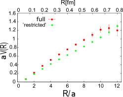
Figure 1: The static potential between the sources in the adjoint representation of $SU(2)$ using eq. 10 for $j=1$ and for comparison the full Wilson loop average in the adjoint representation. The result is consistent with that of [11, 13] where the same quantity is calculated by the Abelian projection method.

In case of the $SU(2)$, we investigate the Wilson loop in the adjoint representation $\mathbf{3}$ ($j=1$). The restricted field, the extracted dominant mode for confinement, is obtained by using the decomposition eq(4) for the color field which minimizes the reduction condition Eq(5)($N=2).$ Figure 1 shows that the string tension from the restricted and Yang-Mills filed in the adjoint represent are in good agreement.

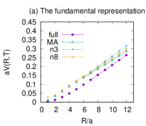
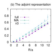
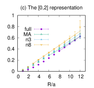
Figure 2: The static potential from the Wilson loop average $\left\langle W_{R}(R,T=8)\right\rangle$ in the representation $R$ of $SU(3)$ calculated using eq. 11: (a) fundamental $[1,0]$ Rep., (b) adjoint $[1,1]$ Rep. , and sextet $[0,2]$ Rep. in comparison with the full Wilson loop average. The legends, MA, n3, and n8, represents the mesurements by using the corresponding reduction conditions, Eqs(5), (6), and (7), respsctively.

	full	MA	n3	n8
fundamental	$0.02776(2)$	$0.02458(1)$	$0.02884(3)$	$0.02544(3)$
adjoint	$0.0576(1)$	$0.0522(1)$	$0.062(1)$	$-$
[0,2]	$0.0647(1)$	$0.05691(9)$	$0.0635(2)$	$0.0641(6)$

Table 1: The string tensions in the lattice unit in the $SU(3)$ case: the string tensions obtained under the MA gauge (5), and reduction conditions n3 (6) and n8 (7), in comparison with the full string tension.

In case of $SU(3)$ we investigate the Wilson loop eq(11), i.e., (a) in the fundamental representation $[0,1]=\mathbf{3}$, (b) in the adjoint representation $[1,1]=\mathbf{8}$, and (c) in the sextet representation $[0,2]=\mathbf{6}$. For each representation, we measure the Wilson loop average for possible reduction conditions, eq(5) ($N=3)$, eq(6), and eq(7).  Figure 2 shows the static potentials from the Wilson loop in the higher representations. Table 1 shows the string tensions which are extracted by fitting the data with the linear potential for the infrared region. The string tensions extracted from our proposed ”dominant” operators reproduce nearly equal to or more than $80\%$ of the full string tension. These results indicate that the proposed operators give actually the dominant part of the Wilson loop average.

5 Conclusion

We have proposed a solution for the problem that the correct behavior of the Wilson loop in higher representations cannot be reproduced if the restricted part of the Wilson loop is naively extracted by adapting the Abelian projection or the field decomposition in the same way as in the fundamental representation. We have proposed the prescription to construct the operator suitable for this purpose. We have performed numerical simulations to show that this prescription works well in the adjoint rep. for $SU(2)$ color group, and in the fundamental, adjoint , and sextet representations for $SU(3)$ color group. Further studies are needed in order to establish the magnetic monopole dominance in the Wilson loop average for higher representations, supplementary to the fundamental representation for which the magnetic monopole dominance was established.

References

- [1] Y. Nambu, Phys. Rev. D10 (1974) 4262 ; G. ’t Hooft, in High Energy Physics, Editorice Compositori, Bologna, 1975; S. Mandelstam, Phys. Rept. 23 (1976) 245 .
- [2] G. ’t Hooft, Nucl. Phys. B 190 (1981) 455 .
- [3] Y. S. Duan, M. L. Ge, Sinica Sci. 11 (1979) 1072; Y. M. Cho, Phys. Rev. D 21 (1980) 1080.
- [4] K.-I. Kondo, S. Kato, A. Shibata and T. Shinohara, Phys. Rept. 579 (2015) 1 [arXiv:1409.1599] .
- [5] R. Matsudo, K.-I. Kondo, Phys.Rev. D 92 (2015) no.12, 125038
- [6] D. Diakonov and V. Petrov, Phys. Lett. B 224 (1989) 131 .
- [7] T. Suzuki and I. Yotsuyanagi, Phys. Rev. D 42 (1990) 4257.
- [8] H. Shiba and T. Suzuki, Phys. Lett. B 333 (1994) 461.
- [9] J. D. Stack, W. W. Tucker and R. J. Wensley, Nucl. Phys. B 639 (2002) 203.
- [10] L. Del Debbio, M. Faber, J. Greensite and S. Olejnik, Phys. Rev. D 53 (1996) 5891.
- [11] G. Poulis, Phys. Rev. D 54 (1996) 6974.
- [12] G. Bali, C. Schlichter and K. Schilling, Phys. Rev. D 51 (1995) 5165.
- [13] M. N. Chernodub, K. Hashimoto and T. Suzuki, Phys. Rev. D 70 (2004) 014506.