Gravitational Wave Emission from 3D Explosion Models of Core-Collapse Supernovae with Low and Normal Explosion Energies

Abstract

Understanding gravitational wave emission from core-collapse supernovae will be essential for their detection with current and future gravitational wave detectors. This requires a sample of waveforms from modern 3D supernova simulations reaching well into the explosion phase, where gravitational wave emission is expected to peak. However, recent waveforms from 3D simulations with multi-group neutrino transport do not reach far into the explosion phase, and some are still obtained from non-exploding models. We therefore calculate waveforms up to 0.9 s after bounce using the neutrino hydrodynamics code CoCoNuT-FMT. We consider two models with low and normal explosion energy, namely explosions of an ultra-stripped progenitor with an initial helium star mass of $3.5\,M_{\odot}$, and of an $18\,M_{\odot}$ single star. Both models show gravitational wave emission from the excitation of surface g-modes in the proto-neutron star with frequencies between $\mathord{\sim}800\,\mathrm{Hz}$ and 1000 Hz at peak emission. The peak amplitudes are about $6\,\mathrm{cm}$ and $10\,\mathrm{cm}$, respectively, which is somewhat higher than in most recent 3D models of the pre-explosion or early explosion phase. Using a Bayesian analysis, we determine the maximum detection distances for our models in simulated Advanced LIGO, Advanced Virgo, and Einstein Telescope design sensitivity noise. The more energetic $18M_{\odot}$ explosion will be detectable to about $17.5\,\mathrm{kpc}$ by the LIGO/Virgo network and to about $180\,\mathrm{kpc}$ with the Einstein Telescope.

1 Introduction

The gravitational wave signal emitted by a core-collapse supernova (CCSN) explosion is expected to be in the detectable frequency range of ground based gravitational wave detectors such as Advanced LIGO (aLIGO; The LIGO Scientific Collaboration et al., 2015) and Advanced Virgo (AdVirgo; Acernese & et al., 2015). At present, the explosion mechanism of CCSNe is still not fully understood. The shock wave formed during the core bounce stalls at a radius of $\sim 150\,\mathrm{km}$ and energy is needed to revive the shock. The current prevailing theory is known as the neutrino-driven mechanism (Janka, 2012; Burrows, 2013), which involves the re-absorption of a fraction of the emitted neutrinos to heat the post-shock matter, revive the shock, and power the explosion.

Accurate three-dimensional (3D) CCSN simulations will be essential for understanding the expected gravitational wave signal and will improve the prospects for detection and astrophysical interpretation of the source. Understanding the time-frequency structure will allow tuning of gravitational wave searches and parameter estimation (Torres-Forné et al., 2018; Powell et al., 2017; Powell et al., 2016; Gill et al., 2018; Gossan et al., 2016). The structure of the gravitational wave signal and the problem of parameter estimation has already been very thoroughly investigated in the case of the rotational bounce signal (see Dimmelmeier et al., 2008; Abdikamalov et al., 2014; Kotake, 2013; Kotake & Kuroda, 2017, and references therein). In this case, the amplitude and frequency can be directly related to the rotational properties of the core (Dimmelmeier et al., 2008; Abdikamalov et al., 2014; Richers et al., 2017; Scheidegger et al., 2010) and the frequency of the fundamental quadrupole mode of the proto-neutron star (PNS) (Fuller et al., 2015), which depends on the nuclear equation of state. However, rapidly-rotating progenitors are expected to occur in only a small fraction of all CCSNe (Beck et al., 2012; Mosser et al., 2012).

For a generic CCSN, one expects the gravitational wave emission to be dominated by hydrodynamic instabilities in the post-bounce phase such as turbulent convection in the neutrino heating region and inside the PNS (Herant et al., 1994; Burrows et al., 1995; Janka & Müller, 1995), and the standing accretion shock instability (SASI; Blondin et al., 2003; Blondin & Mezzacappa, 2006; Foglizzo et al., 2007). The gravitational wave signal from these instabilities has been thoroughly investigated in axisymmetric (2D) models (Murphy et al., 2009; Yakunin et al., 2010; Müller et al., 2013; Yakunin et al., 2015; Morozova et al., 2018), which have established that the most dominant feature in the time-frequency structure of the signal is the quadrupolar surface g-mode of the PNS, which is excited by the hydrodynamical instabilities inside and outside the PNS. The gravitational wave emission from the surface g-modes is emitted at high frequencies of several hundred Hz and rises monotonically in time due to the contraction of the PNS (Murphy et al., 2009; Müller et al., 2013; Cerdá-Durán et al., 2013; Andresen et al., 2017; Kuroda et al., 2016); it may thus allow us to infer properties of the PNS without fully understanding the expected time series of CCSN gravitational wave signals (Torres-Forné et al., 2018).

The gravitational waveforms for the post-bounce signal from 2D simulations are problematic, however, since significant differences have been identified between 2D and 3D models in the post-bounce phase (Andresen et al., 2017). Some gravitational wave signal predictions from 3D simulations of neutrino-driven explosions have recently become available (Andresen et al., 2017; Yakunin et al., 2017; Takiwaki & Kotake, 2018; Yakunin et al., 2017; Kuroda et al., 2016; Andresen et al., 2019). The high-frequency signal from the surface g-mode appears considerably weaker in 3D (Andresen et al., 2017). In addition, the latest 3D simulations find that the SASI produces features in the gravitational wave signal at low frequencies (below 200 Hz), which is the most sensitive frequency range of current ground based gravitational wave detectors.

The corpus of gravitational waveforms from 3D simulations of the post-bounce phase is still small, however, and a number of better waveforms are still needed for many reasons: Both parameterised 3D models (Müller et al., 2012) and self-consistent 2D models (Müller et al., 2013) have shown that gravitational wave emission from neutrino-driven convection peaks after shock revival, yet the signal predictions from self-consistent, state-of-the-art 3D simulations (Yakunin et al., 2017; Andresen et al., 2017, 2019) do not reach far into the explosion phase, and may thus underestimate the peak amplitudes and total power of the signal. Moreover, the predicted amplitudes and the characteristic frequencies differ widely; for example Yakunin et al. (2017) find considerably larger amplitudes than Andresen et al. (2017) and O’Connor & Couch (2018). The time-frequency structure of some models (Andresen et al., 2017) is not completely clear because of aliasing problems. Some waveforms in Andresen et al. (2017) and O’Connor & Couch (2018) are from non-exploding models and may therefore have unrealistically weak gravitational wave emission. Finally, many 3D simulations use pseudo-Newtonian codes that systematically overpredict gravitational wave frequencies (Müller et al., 2013). We therefore seek to generate new waveforms from general-relativistic 3D long-time explosion models with fine time resolution across the mass range of supernova progenitors.

In this study, we perform 3D simulations of two different progenitors to this end, and analyse the detectability of the predicted waveforms by current and third-generation gravitational wave detectors. The first progenitor is an ultra-stripped star simulated from an initial helium star of mass $3.5\,M_{\odot}$ in Tauris et al. (2015), which we refer to as model He3.5. An ultra-stripped star is a binary star that has become an almost naked metal core due to mass transfer via Roche-lobe overflow to the binary companion (Tauris et al., 2015, 2013). Although supernovae from stripped-envelope progenitors in binary systems are of interest in their own right because most massive stars are located in binaries (Chini et al., 2012) and a large fraction of them interact with their companion (Sana et al., 2013), this model primarily serves as a representative example for a supernova with modest explosion energy (Müller et al., 2019). The second progenitor is an $18\,M_{\odot}$ star. This more massive progenitor is representative for supernovae with higher, more typical explosion energies around $10^{51}\,\mathrm{erg}$ and stronger gravitational wave emission. Since more energetic supernovae are expected to have stronger gravitational wave emission (Müller et al., 2013), these two progenitors allow us to better assess the range of gravitational wave amplitudes from successful explosion models. Aside from producing gravitational waveforms that reach further into the explosion phase, another thrust of our paper is to shed more light on the dynamics of the PNS convection, which has been found to be crucial for the excitation of the PNS surface g-mode in 3D (Andresen et al., 2017), and whose relation to the lepton-number emission self-sustained asymmetry (LESA; Tamborra et al., 2014) is still not well understood.

The outline of our paper is as follows: Section 2 gives a brief outline of our numerical methods and set up. In Section 3, we describe the models that are simulated in this study. In Section 4, we discuss the explosion dynamics of our models and compare to previous simulations. In Section 5, we describe and analyse the dynamics of the PNS convection zone and discuss the features of the LESA instability observed in our models. The features of the gravitational wave emission are described in Section 6. We explore the detectability of our gravitational wave signals in Section 7, and a discussion and conclusions are given in Section 8.

2 Simulation Methodology and Setup

Our simulations are carried out using the neutrino hydrodynamics code CoCoNuT-FMT. We use a general relativistic finite-volume based solver for the equations of hydrodynamics (Müller et al., 2010; Dimmelmeier et al., 2002) formulated in spherical polar coordinates. Different from previous 3D simulations with CoCoNuT-FMT, we simulate in 3D down to the innermost $\sim 10$ km to include the PNS convection zone and impose spherical symmetry inside this radius. The neutrino transport is handled using the fast multigroup transport method of Müller & Janka (2015) with updates to the neutrino rates to include nucleon potentials (Martínez-Pinedo et al., 2012), nucleon correlations in the virial approximation (Horowitz et al., 2017), weak magnetism (Horowitz, 2002), and a nucleon strangeness of $g_{A}=-0.05$, which is roughly compatible with current experimental constraints and theoretical expectations (Hobbs et al., 2016). To keep the computational costs manageable despite resolving the PNS convection zone in 3D, we adopt a coarser grid in energy space with only 9 energy groups (instead of the usual 21 energy groups in our recent models).

We implemented on-the-fly extraction of gravitational waves with fine temporal sampling, by means of the modified time-integrated quadrupole formula for strong fields as described in Müller et al. (2013).

At high density, we use the equation of state from Lattimer & Swesty (1991) with a bulk incompressibility of K=220 MeV, and the standard treatment of the low-density regime in CoCoNuT-FMT with an equation of state for photons, electrons, positrons, and an ideal gas of nuclei together with a flashing treatment for nuclear reactions (Rampp & Janka, 2002).

3 Supernova Models

We simulate the explosion of two different models, namely model He3.5, an ultra-stripped star (Tauris et al., 2015) with a modest explosion energy of $\mathord{\sim}0.3$ Bethe (Müller et al., 2019), and model s18, an $18\,M_{\odot}$ single-star progenitor with a higher, more typical explosion energy of $\mathord{\sim}0.8$ Bethe (Müller et al., 2017). We refer to the original simulations of Müller et al. (2017) and Müller et al. (2019), as s18-old and He3.5-old to differentiate them from the new models calculated with the setup described in Section 2.

3.1 Model He3.5

Model He3.5 is an ultra-stripped star that was evolved from a helium star with an initial mass of $3.5\,M_{\odot}$ (Tauris et al., 2015). The model was evolved with the binary evolution code BEC (Wellstein et al., 2001) to simulate the later phases of mass loss in the ultra-stripped supernova channel. The pre-collapse mass of the star is $2.6\,M_{\odot}$. Our simulations cover the region inside $10^{5}\,\mathrm{km}$, as the envelope outside this region does not change on the timescale of seconds. During the collapse and the early post-bounce phase, we simulate the interior of the PNS at densities $\mathord{>}10^{11}\,\mathrm{g}\,\mathrm{cm}^{3}$ in spherical symmetry using a mixing-length treatment as in Müller (2015); up to that point, no gravitational wave amplitudes are computed. The region outside is always simulated in 3D. We extend the 3D region to include the PNS convection zone and reduce the spherically symmetric inner domain to a radius of $10\,\mathrm{km}$ when we restart the simulation 0.05 s after core bounce. The simulation is stopped at 0.7 s after core bounce. Aside from the lower energy resolution, the only other difference between model He3.5 and He3.5-old is the inclusion of weak magnetism in He3.5.

3.2 Model s18

Model s18 is a solar metallicity progenitor star with a zero-age main sequence (ZAMS) mass of $18\,M_{\odot}$, and a helium core mass of $5.3\,M_{\odot}$. The last minutes of oxygen shell burning were simulated in 3D (Müller et al., 2016) to properly initialise the aspherical seed perturbations that are critical for shock revival for this model (Müller et al., 2017). Although model s18 has been simulated previously in Müller et al. (2017), the gravitational wave signal was not calculated as the PNS convection zone, which is the main emission region for gravitational waves, was simulated in spherical symmetry. We restart the simulation with a full 3D treatment of PNS convection 0.08 s after the core bounce and stop the simulation at 0.89 s after core bounce. Model s18 also differs from s18-old in that we include strangeness corrections, nucleon correlations, and weak magnetism.

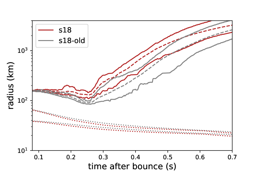
Figure 1: The minimum, maximum, and average shock radius (solid lines) and the radii corresponding to densities of $10^{11}\mathrm{g}\,\mathrm{cm}^{-3}$ and $10^{12}\mathrm{g}\,\mathrm{cm}^{-3}$ (dotted lines, tracking the contraction of the PNS surface) for model s18 (right) and model He3.5 (left). The gray lines show the results from previous simulations, and the red lines show the results from our models. Model He3.5 explodes much later than the previous simulation and has a smaller shock radius. Model s18 explodes slightly earlier than the previous simulation and has a larger shock radius.

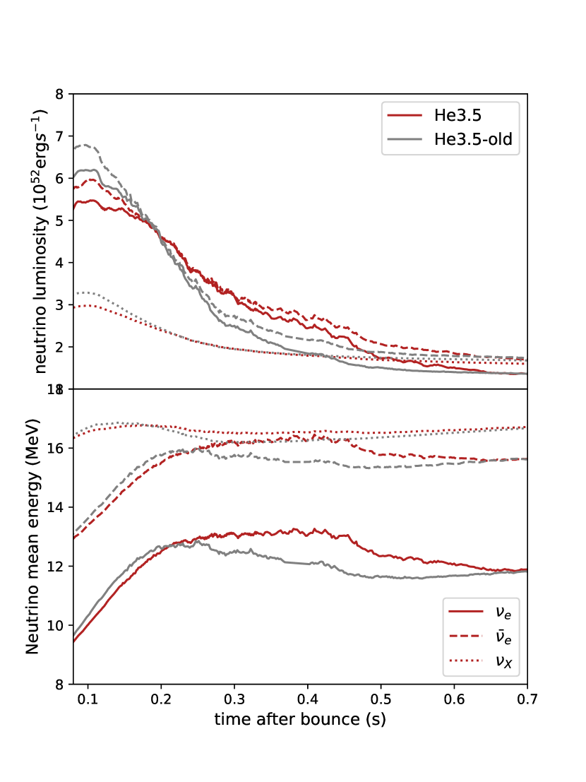
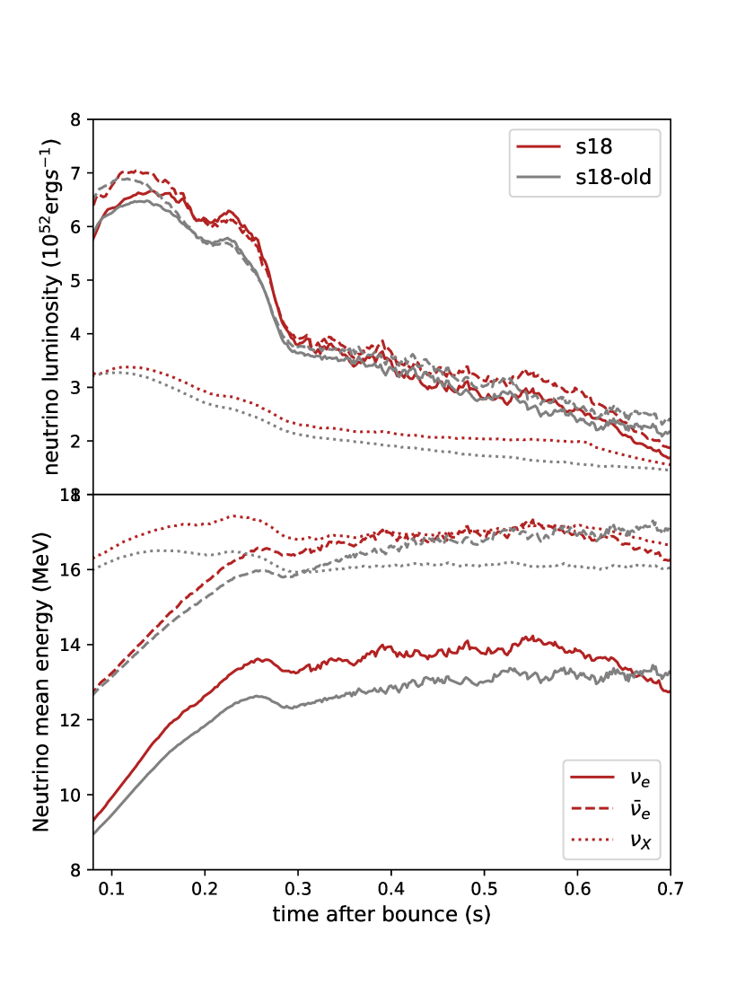
Figure 2: Neutrino luminosities (top) and mean energies (bottom) of $\nu_{e}$ (solid), $\bar{\nu}_{e}$ (dashed), and heavy flavour neutrinos $\nu_{X}$ (dotted) for model s18 (right) and model He3.5 (left) compared to the published models s18-old and He3.5-old. The gray lines show the results from previous simulations, and the red lines show the results from our models. Model He3.5 has lower neutrino luminosity than He3.5-old within the first 0.2 s, and higher neutrino luminosity at later times than the previous simulation. Model s18 has higher neutrino energies than model s18-old.

4 Explosion Dynamics and Comparison with Previous Simulations

Even though the two progenitors have already been simulated in 3D with the CoCoNuT-FMT code, it is useful to briefly outline the dynamical evolution of both models as background information for understanding the gravitational wave signals. Moreover, since we changed several elements of the simulation setup, we briefly compare our models to the corresponding simulations of Müller et al. (2019) and Müller et al. (2017). Although we cannot disentangle the individual effects of the full 3D treatment of PNS convection, the improved neutrino opacities, and the reduced resolution in energy space, it is important to verify that the new simulations remain qualitatively and quantitatively similar to the old models. It is especially important that the physical parameters affecting the gravitational wave emission are not unduly affected by the reduced energy resolution.

The shock radius and the radii corresponding to densities of $10^{11}\mathrm{g}\,\mathrm{cm}^{-3}$ and $10^{12}\mathrm{g\,cm}^{-3}$ are shown in Figure 1 for both models. Models He3.5 and He3.5-old both explode due to the relatively steep decline of the mass accretion rate that is characteristic of stars with low-mass helium cores. However, the shock is revived considerably later in model He3.5 than in He3.5-old, and the shock radius remains significantly smaller from 0.2 s after core bounce onward. PNS contraction is slightly slower in He3.5 than in He3.5-old.

Model s18 undergoes explosion $\mathord{\sim}250\,\mathrm{ms}$ after bounce aided by the infall of strong seed perturbations from the O shell. The simulation produced in this paper shows a slightly larger shock radius than s18-old, and the shock is revived $\mathord{\sim}5\,\mathrm{ms}$ earlier. The PNS contracts slightly faster in s18 than in s18-old.

The differences in the evolution of model s18 vis à vis s18-old and He3.5 vis à vis He3.5-old are explained by differences in the neutrino emission that result from the changes in energy resolution and the opacities. The neutrino luminosities and mean energies for all models are shown in Figure 2. For the $18\,M_{\odot}$ progenitor, the changes in energy resolution and neutrino interaction rates result in increased luminosities and mean energies of all neutrino flavours. This naturally explains the slightly earlier onset of the explosion and the larger stagnation of the shock radius prior to shock revival. Since the infall of the Si/O shell interface and the presence of pre-shock perturbations in the O shell play a major role in triggering shock revival, the higher neutrino luminosities and mean energies cannot shift the onset of the explosion appreciably, however, and hence the shock trajectories of models s18 and s18-old remain similar during the explosion phase. The somewhat faster propagation of the shock in s18 helps to quench accretion onto the PNS, and as the result of the slightly faster decline of the accretion luminosity, the neutrino emission in model s18 again becomes more similar to s18-old later in the explosion phase.

The increased neutrino luminosities and mean energies in model s18 likely result from a combination of effects. Both the strangeness correction for neutrino-nucleon scattering (Melson et al., 2015) and nucleon correlations (Horowitz et al., 2017; Bollig et al., 2017) tend to increase neutrino luminosities and mean energies and lead to faster PNS contraction. This effect may be compounded by the low energy resolution. Only a few studies have addressed the role of resolution in energy space, but it is clear that nine energy groups are not sufficient to fully resolve the neutrino spectrum and easily introduce uncertainties of a few percent in the luminosities (Marek, 2007).

The results for models He3.5 and He3.5-old confirm that energy resolution is a major factor. Figure 2 shows a significant reduction of the neutrino luminosities of all flavours on the 10%-level in He3.5-old early on. Although model He3.5 also differs from He3.5-old in that it includes weak magnetism corrections, these corrections do not produce an effect of such magnitude (Buras et al., 2006a; Fischer et al., 2018), and do not affect the heavy flavour neutrino in our simulations since we treat $\nu_{\mu/\tau}$ and their antiparticles $\bar{\nu}_{\mu/\tau}$ as a single species in our code.

Due to the relatively large differences in the neutrino emission, shock revival is delayed by about $0.2\,\mathrm{s}$ in model He3.5 compared to He3.5-old. As a result of ongoing accretion, higher neutrino luminosities and mean energies are maintained in model He3.5 from a post-bounce time of $0.2\,\mathrm{s}$ until about $0.65\,\mathrm{s}$. Moreover, the PNS radius is slightly larger in model He3.5.

From this cursory analysis, it is clear that the energy resolution and the details of the microphysics have an important bearing on the detailed neutrino emission. This is, however, not our primary concern here. What is important for our purpose is rather whether the models predict the physical parameters relevant for the gravitational wave emission with reasonable robustness. Especially for model s18, this appears to be the case: Despite differences in energy resolution and in the microphysics, models s18 and s18-old exhibit very similar explosion dynamics. The factors that determine the frequency $f_{\mathrm{g}}$ of the surface g-mode that dominates the gravitational wave spectrum (Murphy et al., 2009; Müller et al., 2013) are also similar. In terms of the baryonic neutron star mass $M_{\mathrm{by}}$, the neutron star radius $R$, the electron antineutrino mean energy $\langle E_{\bar{\nu}_{\mathrm{e}}}\rangle$, and the neutron mass $m_{n}$ one one finds (Müller et al., 2013),

$$f_{\mathrm{g}}\approx\frac{1}{2\pi}\frac{GM_{\mathrm{by}}}{R^{2}}\sqrt{1.1\frac{m_{\mathrm{n}}}{\langle E_{\bar{\nu}_{\mathrm{e}}}\rangle}}\left(1-\frac{GM_{\mathrm{by}}}{Rc^{2}}\right).$$ (1)

As discussed before, $\langle E_{\bar{\nu}_{\mathrm{e}}}\rangle$ and $R$ do not differ greatly between models s18 and s18-old, and the PNS masses are also similar; the final baryonic PNS mass $M_{\mathrm{by}}$ is lower by $0.06\,M_{\odot}$ in model s18 due to somewhat faster quenching of the accretion. Hence we expect the frequency of the surface g-mode to be reliable within a few percent despite the reduced energy resolution in model s18.

The case of the $3.5\,M_{\odot}$ stripped-envelope progenitor is slightly different because the explosion dynamics of model He3.5 differs appreciably from He3.5-old. When interpreting the gravitational wave amplitudes, it must be borne in mind that there is considerably uncertainty about the time of shock revival in this model. There is less of a concern about the gravitational wave spectra, however. Although the neutrino mean energies differ by up to $\mathord{\sim}10\%$ between He3.5 and He3.5-old (as a result of the delayed onset of the explosion), the PNS contraction is similar, as is the PNS mass, which is only $0.03\,M_{\odot}$ higher in He3.5 at the end of the simulation. Since the electron antineutrino mean energy only enters in $f_{\mathrm{g}}$ as $\langle E_{\bar{\nu}_{\mathrm{e}}}\rangle^{-1/2}$, the surface g-mode frequency in model He3.5 is still reliable within a few percent.

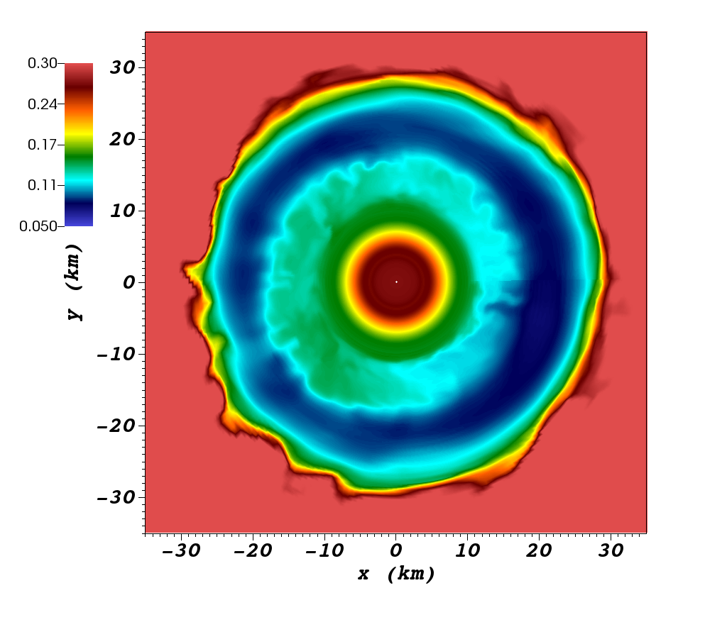
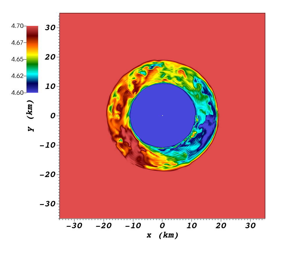
Figure 3: Two-dimensional slices through the PNS convection zone in model s18 showing the electron fraction (top), the entropy in units of $k_{\mathrm{b}}/\mathrm{nucleon}$ (middle), and the radial velocity in units of $\mathrm{km}\,\mathrm{s}^{-1}$ at a post-bounce time of $453\,\mathrm{ms}$.

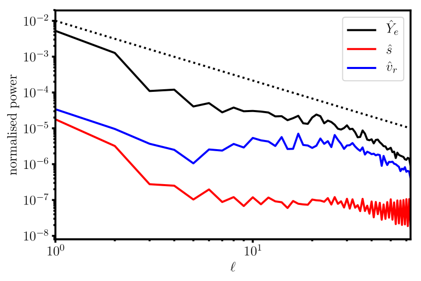
Figure 4: Spectra of the normalised perturbations in electron fraction ($\hat{Y}_{e,\ell}/\hat{Y}_{e,0}$, black), entropy ($\hat{s}_{e,\ell}/\hat{s}_{e,0}$, black) and the radial Mach number ($\hat{v}_{r,\ell}/\hat{c}_{s,0}$, blue) in the PNS convection zone at a radius of $13.7\,\mathrm{km}$ and at a post-bounce time of $454\,\mathrm{ms}$ for model s18. The slope of a Kolmogorov spectrum with a power law of $-5/3$ is indicated as a dotted line.

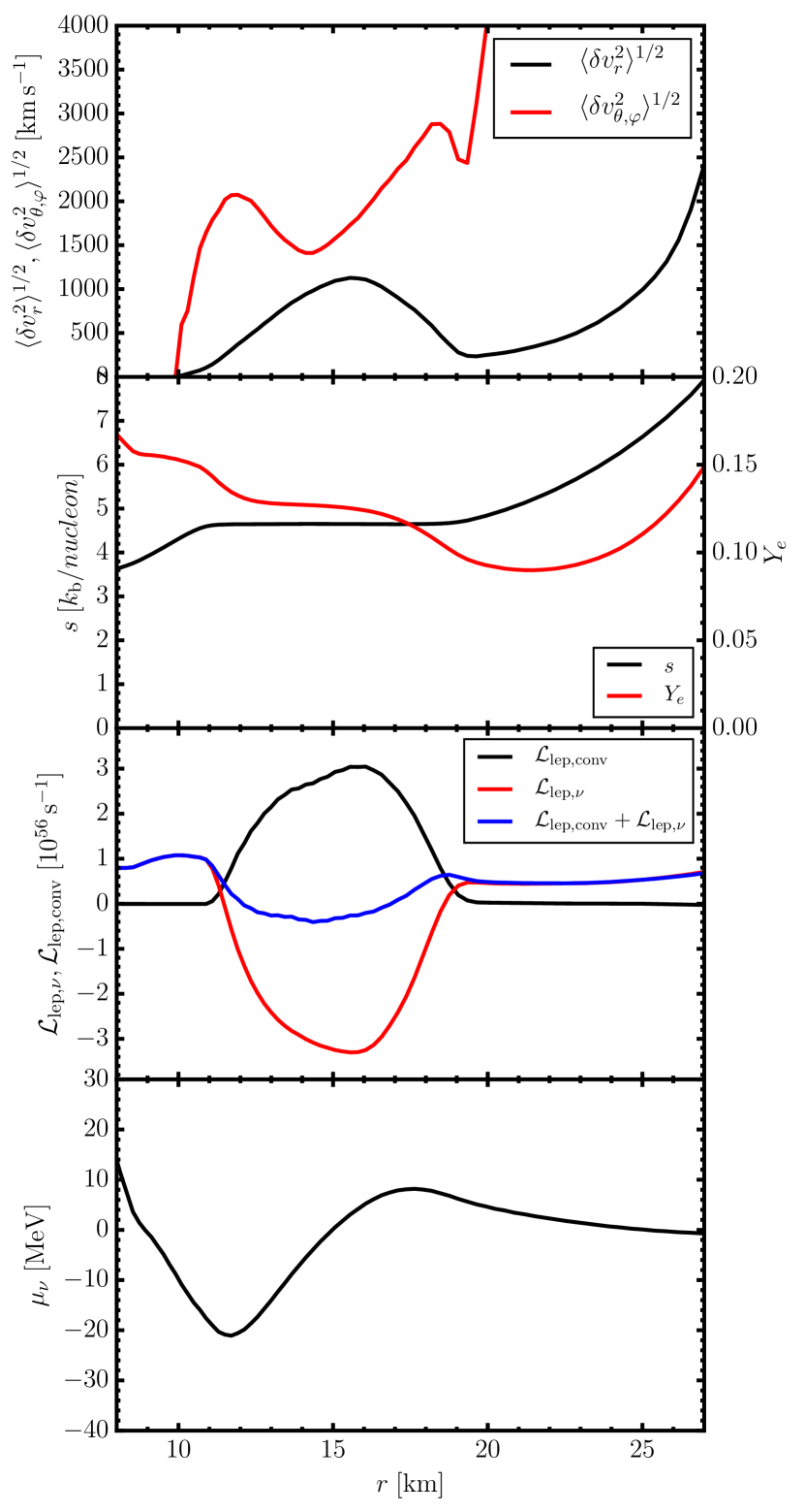
Figure 5: RMS averages of the radial and non-radial velocity fluctuations (panel 1), angle-averaged profiles of the entropy $s$ and the electron fraction $Y_{e}$ (panel 2), convective and diffusive lepton number luminosities $\mathcal{L}_{\mathrm{\mathrm{lep},\mathrm{conv}}}$ and $\mathcal{L}_{\mathrm{\mathrm{lep},\nu}}$ and their sum (panel 3), and neutrino chemical potential $\mu_{\nu}$ (panel 4) in the PNS convection zone for model s18 at a post-bounce time of $454\,\mathrm{ms}$.

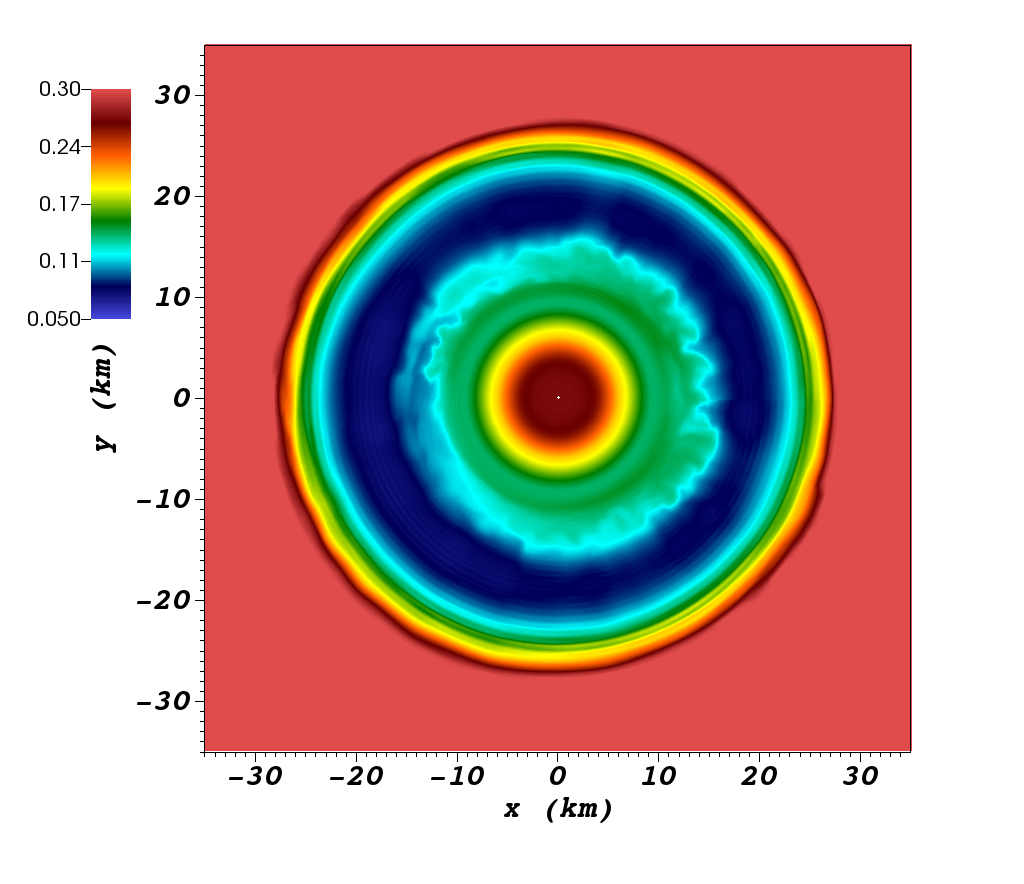
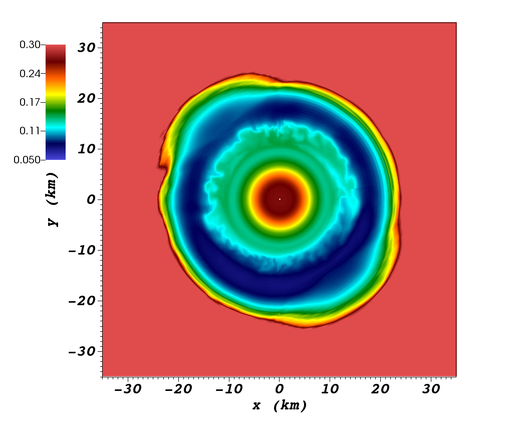
Figure 6: Two-dimensional slices through the PNS convection zone showing the electron fraction in models s3.5 (top) and s18 (bottom) towards the end of the simulations.

5 Features of Proto-Neutron Star Convection

In their study of gravitational wave emission in 3D supernova models, Andresen et al. (2017) concluded that PNS convection is the primary driver of the PNS surface g-modes that dominate the high-frequency gravitational wave spectrum. Although multi-dimensional simulations of PNS convection initially suggested a relatively straightforward picture of PNS convection as simple Ledoux convection (Keil et al., 1996; Buras et al., 2006b; Dessart et al., 2006), the fluid motions in the PNS convection zone have proved more enigmatic in recent years. While the extent of the unstable region is well described by the Ledoux criterion and quite consistent between different codes, significant variations in the convective velocities have recently been reported in a cross-comparisons of the Vertex and Alcar codes (Just et al., 2018). Moreover, many of the recent 3D models develop a peculiar hemispheric lepton number asymmetry in the PNS convection zone as first discovered and termed LESA (“Lepton-number Emission Self-sustained Asymmetry”) instability by Tamborra et al. (2014); this has recently been confirmed in other 3D simulations using different codes (O’Connor & Couch, 2018; Glas et al., 2018). Independently of computational studies of PNS convection, the role of double-diffusive instabilities (Bruenn & Dineva, 1996) in the PNS convection zone has long been discussed, but no phenomenon in multi-D simulations has yet been connected to such instabilities. What precisely determines the flow pattern and the convective velocities in the PNS interior is thus by no means completely understood.

Before we proceed to analysing the gravitational wave emission itself, it is therefore worthwhile to study the properties of PNS convection in our 3D models and compare the findings to other recent simulations. Since all of the qualitative features of PNS convection turn out to be in agreement with the studies of Tamborra et al. (2014); O’Connor & Couch (2018); Glas et al. (2018), we mostly confine our analysis to model s18 and to one representative epoch.

Figure 3 shows the electron fraction $Y_{e}$, the specific entropy $s$, and the radial velocity $v_{r}$ on two-dimensional slices through model s18 at a post-bounce time of $454\,\mathrm{ms}$. LESA is clearly present, with a pronounced dipolar asymmetry in the electron fraction $Y_{e}$ (top panel). While previous studies of LESA have not addressed asymmetries in the entropy (which are somewhat hard to diagnose because of the minute dynamic range of entropy fluctuations), the entropy distribution in the PNS convection zone exhibits the same dipolar asymmetry in our model. This suggests that LESA is actually not an instability that imprints a global asymmetry specifically on the lepton number distribution. The lepton number asymmetry is merely more prominent because the contrast in electron fraction/lepton number across the PNS convection zone is considerably larger than the entropy contrast. This could suggest that LESA is in effect not a new instability, but merely a manifestation of “normal” convection with the preferred length scales set by the geometry of the unstable region and perhaps finite (physical and numerical) viscosity and diffusivity (Glas et al., 2018). The presence of weak dipole asymmetry in the radial velocity field (again, similar to Glas et al. 2018), superimposed over eddies of smaller scale (bottom panel), would be compatible with this parsimonious interpretation.

A more detailed analysis reveals more complicated dynamics in the PNS convection zone, however. To analyse the spectrum of the convective motions, we consider the power in spherical harmonics of degree $\ell$ for the perturbations in electron fraction, entropy, and radial velocity. For quantity $X$, we compute the power $\hat{X}_{\ell}$ in multipole $\ell$ as

$$\hat{X}_{\ell}=\sum_{m=-\ell}^{\ell}\left|\int Y_{\ell m}^{*}(\theta,\varphi)X(\theta,\varphi)\,\mathrm{d}\Omega\right|^{2}.$$ (2)

It is then useful to normalise the power by the power $\hat{X}_{0}$ in the monopole, or, in case of the radial velocity, by the monopole component $\hat{c}_{\mathrm{s},0}$ of the sound speed. When computing the spectra, we average the power over six radial zones around a radius of $13.7\,\mathrm{km}$.

The normalised spectra $\hat{Y}_{e,\ell}/\hat{Y}_{e,0}$, $\hat{s}_{e,\ell}/\hat{s}_{e,0}$ and $\hat{v}_{r,\ell}/\hat{c}_{s,0}$ are shown in Figure 4. The spectra differ considerably from standard Kolmogorov scaling laws for isotropic turbulence and also from Bolgiano-Obukhov scaling for stratified ideal and viscous flow (Obukhov, 1959; Kumar et al., 2014). The spectra of the electron fraction and entropy do not nicely conform to a power law at low $\ell$ and are suggestive of a deficit of power at angular wave numbers $\ell\sim 3\texttt{-}10$. For the radial velocity, it is even clearer that there are two peaks at $\ell=1$ and $\ell\sim 10$, suggesting that the flow is shaped by two distinct scales. It is also noteworthy that the shape of the velocity spectrum differs from the spectra of $s$ and $Y_{e}$. This is understandable for the wavenumbers that are subject to strong numerical dissipation or (radial) odd-even noise that manifests itself in the high-wavenumber tail of the entropy spectrum, but it is not expected for low and intermediate wavenumbers.

More evidence for complex stratification within the PNS convection zone comes from radial profiles of various thermodynamic quantities and the turbulent velocity fluctuations, and from the turbulent lepton number flux (Figure 5). The angular root-means square averages $\langle\delta v_{r}^{2}\rangle^{1/2}$ and $\langle\delta v_{\theta,\varphi}^{2}\rangle^{1/2}$ of the radial and non-radial velocity fluctuations $\delta v_{r}$ and $\delta v_{\theta,\varphi}$ around their spherical average (top panel) suggest that the well-mixed region extends from about $\mathord{\sim}10\,\mathrm{km}$ to $\mathord{\sim}19\,\mathrm{km}$. While the entropy profile is almost perfectly flat within this region (second panel), the profile of $Y_{e}$ exhibits a much narrower plateau in the middle of the convective zone, and broad “steps” at the outer and inner convective boundary. Especially at the outer boundary, this step clearly starts already well within the convection zone. This $Y_{e}$-profile is maintained as the result of convective and diffusive transport counteracting each other. The third panel in Figure 5 illustrates that through most of the PNS convection zone, the net lepton number luminosity $\mathcal{L}_{\mathrm{lep},\nu}$ carried by diffusing neutrinos is actually negative and almost cancels the convective lepton number luminosity $\mathcal{L}_{\mathrm{\mathrm{lep},\mathrm{conv}}}$, which we compute as

$$\mathcal{L}_{\mathrm{\mathrm{lep},\mathrm{conv}}}=\int\rho W\delta v_{r}\,\delta Y_{e}\alpha\phi^{4}r^{2}\,\mathrm{d}\Omega.$$ (3)

Here $\rho$, and $W$ are the baroynic mass density and the Lorentz factor, $\delta v_{r}$ and $\delta Y_{e}$ are the fluctuations of the radial velocity and electron fraction computed from a spherical Favre decomposition, and $\alpha$ and $\phi$ are the lapse function and conformal factor in the xCFC metric.

The negative diffusive lepton number flux is the consequence of a positive gradient in the neutrino chemical potential $\mu_{\nu}$ that develops in a wide layer within the convective region (bottom panel of Figure 5). The positive gradient in $\mu_{\nu}$ is also noteworthy because it is a direct reflection of the well-established finding (Lattimer & Mazurek, 1981; Keil et al., 1996; Bruenn & Dineva, 1996; Bruenn et al., 2004; Buras et al., 2006b) that negative lepton number gradients tend to stabilise the stratification against convection in some parts of the convective region. Lattimer & Mazurek (1981) showed that the more familiar form of the Ledoux criterion for convective instability in the presence of entropy and lepton number (electron fraction),

$$\left(\frac{\mathrm{\partial}\rho}{\mathrm{\partial}s}\right)_{Y_{e},P}\frac{\mathrm{d}s}{\mathrm{d}r}+\left(\frac{\mathrm{\partial}\rho}{\mathrm{\partial}Y_{e}}\right)_{s,P}\frac{\mathrm{d}Y_{e}}{\mathrm{d}r}>0,$$ (4)

can be rewritten using the Maxwell relations as

$$\left(\frac{\mathrm{\partial}P}{\mathrm{\partial}s}\right)_{Y_{e},\rho}\frac{\mathrm{d}s}{\mathrm{d}r}+\rho^{2}\left(\frac{\mathrm{\partial}\mu_{\nu}}{\mathrm{\partial}\rho}\right)_{s,Y_{e}}\frac{\mathrm{d}Y_{e}}{\mathrm{d}r}>0.$$ (5)

Thus, negative lepton number gradients become stabilising if

$$\left(\frac{\mathrm{\partial}\mu_{\nu}}{\mathrm{\partial}\rho}\right)_{s,Y_{e}}=\frac{\mathrm{d}\mu_{\nu}}{\mathrm{d}\rho}-\left(\frac{\mathrm{\partial}\mu_{\nu}}{\mathrm{\partial}s}\right)_{\rho,Y_{e}}\frac{\mathrm{d}s}{\mathrm{d}\rho}-\left(\frac{\mathrm{\partial}\mu_{\nu}}{\mathrm{\partial}Y_{e}}\right)_{s,\rho}\frac{\mathrm{d}Y_{e}}{\mathrm{d}\rho}<0.$$ (6)

Since $s\approx\mathrm{const}.$ and $\mathrm{d}Y_{e}/\mathrm{d}\rho>0$ in the PNS convection zone, and since $(\mathrm{\partial}\mu_{\nu}/\mathrm{\partial}Y_{e})_{s,\rho}$ is generally positive, the $\mu_{\nu}$-profile indicates that the negative $Y_{e}$-gradient is stabilising throughout large parts of the convective layer.

Could the stratification of $Y_{e}$ and the stabilising role of the $Y_{e}$-gradient be related to LESA and the peculiar spectra of the convective fluctuations? Double-diffusive instabilities (Bruenn & Dineva, 1996; Bruenn et al., 2004) could in principle lead to considerably different dynamics compared to the familiar Schwarzschild-Ledoux convection. However, since LESA also appears in codes like ours that do not include lateral diffusion and hence do not account for equilibration of rising and sinking fluid elements with their surroundings, double-diffusive instabilities cannot be at the heart of LESA, although they may modify its appearance in detail.

Based on our findings, we speculate that there may nonetheless be a connection to the stabilising role of negative $Y_{e}$-gradients, which may affect convective eddies of various sizes differently: Since the $Y_{e}$-gradient is relatively shallow in a narrow region within the convective zone, small-scale overturn motions in this region would not be strongly affected by stabilising gradients, whereas turnover motions spanning the entire convective region will undergo reduced acceleration by buoyancy forces since the $Y_{e}$-contrast to their surroundings partly negates the higher/lower entropy of rising/sinking bubbles. This might explain the unusually shallow slope of the turbulent velocity spectrum.

Since the $Y_{e}$-gradient in this central layer of the PNS convection zone is shallow, these small-scale overturn motions will be characterized by small $Y_{e}$-contrast, and hence contribute little power to the spectrum of $Y_{e}$ perturbations on small scales. Thus, unlike the spectrum of velocity perturbations, the spectrum $\hat{Y}_{e,\ell}$ will still exhibit a significant slope.

This explanation is only a tentative one, and we will address the structure of PNS convection in more detail in future work. At present our findings mainly serve to highlight the complexity of the LESA phenomenon beyond what has already been described in previous studies. The peculiar features of LESA are also of considerable importance in the context of gravitational wave emission; the power in $\ell=2$ modes that can be seen in gravitational waves is evidently tightly linked to the shape of the turbulence spectra. LESA excites the g-mode oscillations of the PNS that subsequently lead to the high frequency gravitational wave emissions. Further analysis of LESA is thus clearly called for.

It is also worth noting that LESA persists until the end of the simulation in both models (Figure 6), i.e., well into the explosion phase. Since the accretion rate onto the PNS has already dropped significantly by that time, this could be further evidence that the LESA is a phenomenon that arises within the PNS convection itself, rather than depending on a feedback process between the accretion flow and PNS convection as originally envisaged by Tamborra et al. (2014).

6 Gravitational Wave Emission

6.1 Model He3.5

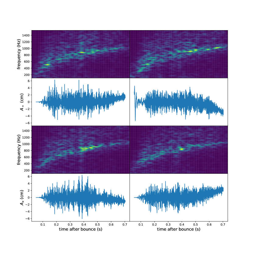
Figure 7: The gravitational wave emission for model He3.5. The left column shows the two polarizations at the pole, and the right column shows the two polarizations calculated at the equator. The frequency peaks between 800 -1000 Hz. The gravitational wave emission peaks after 0.3 s during the revival of the shock. A small tail occurs after 0.5 s.

The gravitational wave emission of model He3.5 is shown in Figure 7. We show the time series and spectrograms for both gravitational wave polarizations for observers at the pole $(\theta,\phi)=(0,0)$ and equator. As expected for a non-rotating simulation, there is a quiescent phase up to $\sim 0.1$ s after core-bounce. At this early time there is a spike in the time series of the plus polarization for an observer at the equator. This occurs because the model is adjusting after we start a 3D treatment of the PNS convection zone after switching from 1D. This is followed by a stochastic phase in the time series. The largest gravitational wave amplitudes, of up to 6 cm, occur after 0.35 s post bounce as the shock is revived and the model enters the explosion phase. The total energy radiated in gravitational waves is $E_{gw}=9.0\times 10^{-10}M_{\odot}c^{2}$ for this model, as given by Equation (22) in Mueller & Janka (1997).

The signal spectrograms show the gravitational wave emission increases in frequency with time as is consistent with the emission expected from g-mode oscillations of the PNS surface. The peak frequency is higher than other recent models at 800 -1000 Hz. Our model has no low frequency emission due to the SASI. This is due to the small core mass and the rapid drop in the accretion rate, similar to the $11.2\,M_{\odot}$ model in Andresen et al. (2017).

A tail in the time series occurs after 0.5 s. The tail is due to anisotropic expansion of the shock wave. A positive amplitude indicates a prolate explosion, and a negative amplitude indicates an oblate explosion (Murphy et al., 2009). Our models show a more pronounced tail signal than any of the other recent 3D models using multi-group neutrino transport (Kuroda et al., 2016; Andresen et al., 2017; Yakunin et al., 2017; Andresen et al., 2019), as these models were not evolved sufficiently far into the explosion phase.

6.2 Model s18

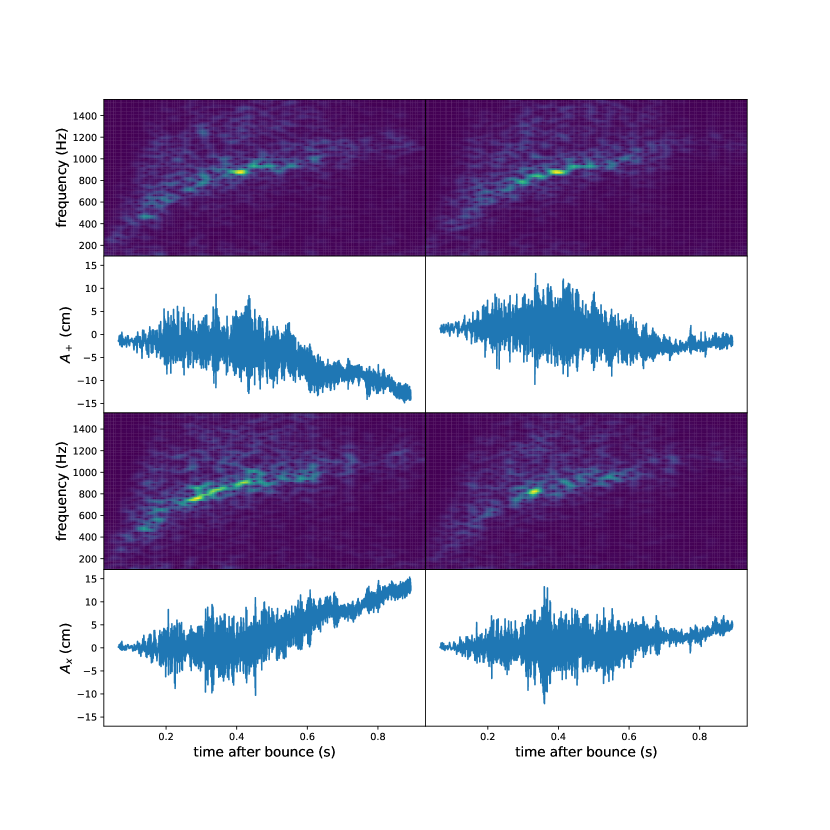
Figure 8: The gravitational wave signal for model s18. As for model He3.5, the left column is the gravitational wave emission at the pole, and the right column is the gravitational wave emission at the equator. The peak gravitational wave emission occurs earlier than for model He3.5 due to the earlier shock revival and has similar peak frequencies between 800 -1000 Hz. This model has a large low frequency tail at late times.

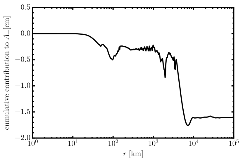
Figure 9: Cumulative contribution of the matter within radius $r$ to the initial offset of the gravitational wave amplitude $A_{+}$ in the polar direction for model s18. The offset is mostly due to the quadrupolar deformation of the collapsing oxygen shell.

The gravitational wave emission produced by model s18 is shown in Figure 8. The model has almost no gravitational wave emission before 0.1 s after core bounce, except for a small negative offset in the plus polarization at the pole. This offset is physical and is due to the fact that the collapsing shells are not spherically symmetric, but inherit a non-negligible quadrupolar deformation from convective burning in the progenitor. By evaluating the cumulative contribution of the region inside radius $r$ in the quadrupole formula (Figure 9), one finds that the offset is mostly due to the quadrupolar deformation from within the violently convective oxygen shell (Müller et al., 2016) between between $r=3000\,\mathrm{km}$ and $r=8000\,\mathrm{km}$, although the shells further inside also become mildly aspherical during the infall and contribute a bit to the offset. The peak gravitational wave emission starts around 0.3 s after core bounce after the revival of the shock. The highest amplitudes continue up to 0.5 s well into the explosion phase. The peak frequency is similar to the previous model, between 800 -1000 Hz, but occurs earlier than model He3.5 due to the earlier explosion time. This model has a larger gravitational wave amplitude than most other recent 3D CCSN simulations with a maximum amplitude of $\sim 10$ cm due to the large mass and high explosion energy of this model of $\sim 0.8$ Bethe. This translates to a gravitational wave energy of $E_{gw}=3.3\times 10^{-9}M_{\odot}c^{2}$.

The gravitational wave emission is due to oscillations of g-modes in the PNS. There is no low frequency emission due to the SASI because of the strong density and pressure perturbations ahead of the shock from convective burning in the oxygen shell. These perturbations disrupt the amplification cycle of vorticity waves and acoustic waves that normally lead to gravitational wave emission produced by the effects of the SASI. This is discussed in more detail in the previous simulation of this model in Müller et al. (2017). There is a large tail in the time series which occurs after 0.45 s.

6.3 The g-mode excitation mechanism and GW strength

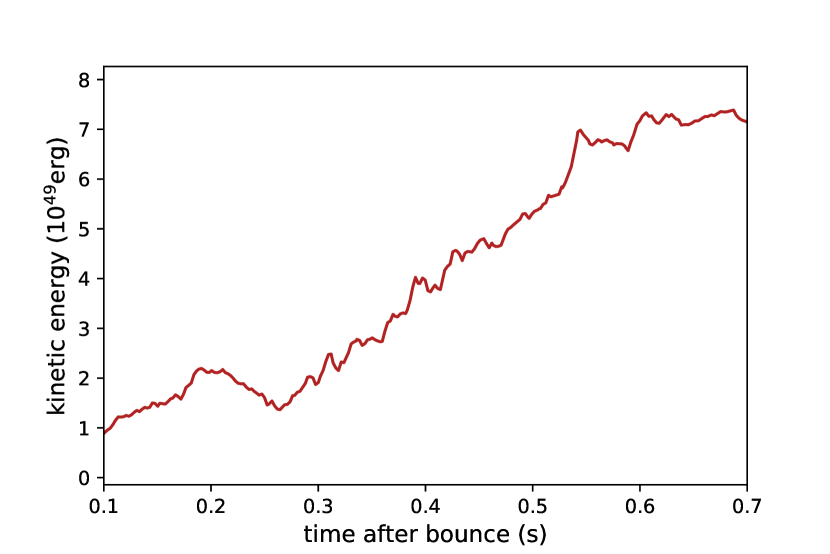
Figure 10: The time evolution of the non-radial kinetic energy contributed from velocity fluctuations in the PNS convection zone for model s18. PNS convection is still energetic after the shock revival phase.

The fact that the high-frequency gravitational wave emission peaks shortly after shock revival in both models and then declines visibly is relevant for the ongoing discussion about the excitation mechanism of the PNS surface g-mode. Andresen et al. (2017) determined that g-modes are predominantly excited by PNS convection, but the rise and decline of the high-frequency emission in our models rather points to a correlation of the emission with the violence of non-radial fluid motions in the gain region, somewhat more similar to 2D explosion models. This is reinforced by the finding that the kinetic energy in non-radial motions inside the PNS convection zone actually grows continuously in model s18 (Figure 10) even while the high-frequency emission is already subsiding. Recently, Radice et al. (2018) also observed such a correlation and found that there is even a relatively tight quantitative relationship between the total energy $E_{\mathrm{GW}}$ of emitted gravitational waves and the time-integrated flux of turbulent kinetic energy $E_{\mathrm{turb}}$ from the gain region onto the PNS,

$$E_{\mathrm{GW}}\approx 3\times 10^{43}\left(\frac{E_{\mathrm{turb}}}{10^{50}\,\mathrm{erg}}\right)^{1.88}.$$ (7)

The disparate findings on the relative contribution of PNS convection and non-radial motions in the gain layer are not at odds with each other, however. It is natural to expect that the relative importance of these two possible drivers of surface g-modes varies across models depending on the violence of non-radial motions in the different unstable regions. One can also derive this more quantitatively (Müller, 2017) by estimating the energy in g-modes using analytic theory, which suggests that the g-mode energy flux $L_{g}$ scales with the convective luminosity $L_{\mathrm{conv}}$ in adjacent convective regions and the convective Mach number $\mathrm{Ma}$ as (Goldreich & Kumar, 1990)

$$L_{g}\sim\mathrm{Ma}\,L_{\mathrm{conv}}.$$ (8)

By assuming that the forcing of the g-modes is coherent over one convective turnover time-scale $\tau$, we can express the energy $E_{g}$ in g-modes in terms of the convective energy $E_{\mathrm{conv}}$ in the forcing motions as (Müller, 2017)

$$E_{g}\sim\mathrm{Ma}\,L_{\mathrm{conv}}\tau\sim\mathrm{Ma}\,(E_{\mathrm{conv}}/\tau)\tau\sim\mathrm{Ma}\,E_{\mathrm{conv}}.$$ (9)

The convective luminosity in the PNS convection zone is of the order of the diffusive neutrino luminosity $L_{\mathrm{core}}$ from the PNS core, which does not vary tremendously across time and progenitors (Mirizzi et al., 2016). The convective luminosity in the gain region, however, scales with the neutrino heating rate $\dot{Q}_{\nu}$ (Murphy et al., 2013; Müller & Janka, 2015),

$$L_{\mathrm{conv}}\sim\dot{Q}_{\nu},$$ (10)

which varies considerably across progenitors and between the pre-explosion and explosion phase. Since $\mathrm{Ma}\,L_{\mathrm{conv}}\tau$ is also of the same order in the PNS convection zone and the gain region (where $L_{\mathrm{conv}}$ is lower by a factor of $\mathcal{O}(10)$, but $\mathrm{Ma}$ and $\tau$ are higher by a factor of several), the relative importance of g-mode excitation by PNS convection and non-radial motions in the gain region is bound to vary quite significantly. If $\mathrm{Ma}$ and $\dot{Q}_{\nu}$ are high – as in our more energetic exploding models and those of Radice et al. (2018) – excitation of g-modes by turbulent motions in the gain region is more likely to dominate than in the pre-explosion phase, which was the primary focus of Andresen et al. (2017).

Even though Equation (9) only provides a very crude model for the interaction between convection and/or SASI and the surface g-mode, it seems to provide a very natural way of interpreting the results on gravitational wave emission from the various recent 3D models (especially Andresen et al. 2017, Radice et al. 2018, and this paper) and naturally explains the scaling relation (7) found by Radice et al. (2018): Using dimensional analysis, one can determine that the typical gravitational wave amplitudes scale with $E_{g}$ as (Müller, 2017)

$$A\sim\frac{\alpha GE_{g}}{c^{4}},$$ (11)

where the dimensionless factor $\alpha$ is of order unity and accounts for the fact that only part of the g-mode energy is stored in quadrupolar modes. If $f$ is the typical emission frequency, the gravitational wave luminosity $\dot{E}_{\mathrm{GW}}$ is roughly

$$\dot{E}_{\mathrm{GW}}\sim\frac{4\pi c^{3}f^{2}A^{2}}{G}.$$ (12)

After integrating over a typical time $T$ of strong emission and inserting Equation (9) for $L_{\mathrm{conv}}$, we obtain $E_{\mathrm{GW}}$ in terms of the time-integrated flux $E_{\mathrm{turb}}=L_{\mathrm{conv}}T$ of turbulent kinetic energy onto the PNS surface as

$$E_{\mathrm{GW}}\sim\frac{4\pi G(f\tau\mathrm{Ma}L_{\mathrm{conv}}T)^{2}}{c^{5}}=\frac{4\pi Gf^{2}\tau^{2}\mathrm{Ma}^{2}E_{\mathrm{turb}}^{2}}{c^{5}}\\ =4.2\times 10^{43}\,\mathrm{erg}\left(\frac{f}{1000\,\mathrm{Hz}}\right)^{2}\left(\frac{\tau}{20\,\mathrm{ms}}\right)^{2}\left(\frac{\mathrm{Ma^{2}}}{0.3}\right)\left(\frac{E_{\mathrm{turb}}}{10^{50}\,\mathrm{erg}}\right)^{2}.$$ (13)

For typical values around shock revival of $\tau=20\,\mathrm{ms}$ (Müller & Janka, 2014) and $\mathrm{Ma}^{2}=0.3$ (Müller & Janka, 2015), the result is very similar to the empirical scaling relationship of Radice et al. (2018) with only a slightly different power-law exponent.

7 Detection Prospects

In this section, we estimate the distance out to which our gravitational wave signals may be detected in current ground-based gravitational wave detectors and a planned next generation underground detector called Einstein Telescope (ET; Punturo et al., 2010). We simulate Gaussian design sensitivity noise for the aLIGO and AdVirgo detectors using the power spectral density (PSD) curves described in Abbott et al. (2018). For ET, we use the ET-B noise curve described in Hild et al. (2008). The noise curves are shown in Figure 11, as well as the maximum amplitude spectral density (ASD) of our models at a distance of 10 kpc. The AdVirgo detector has poor sensitivity above 400 Hz, in the region where our models have the greatest gravitational wave amplitude. The aLIGO detectors have better sensitivity at the higher peak frequencies in our models. In the case of ET, the sensitivity improves over the entire frequency band of our models greatly improving the detection prospects.

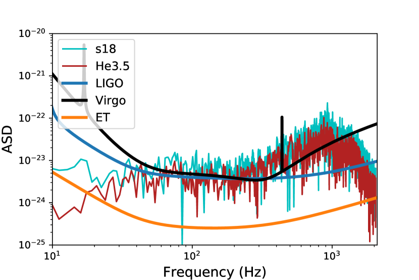
Figure 11: The gravitational wave models at a distance of 10 kpc relative to the design sensitivity amplitude spectral density (ASD) curves of Advanced LIGO, Advanced Virgo, and ET-B, assuming maximum antenna pattern sensitivity of the signals. ET will improve the detection sensitivity across the entire frequency band.

To make an approximate estimation of the distance out to which our waveforms can be detected, we use the Bayesian inference code known as Bilby (Ashton et al., 2019). Bilby is most commonly used as a parameter estimation tool, however the Bayes factors calculated in Bilby can be used as a detection statistic (Smith & Thrane, 2018; Lynch et al., 2017). We use a sine Gaussian signal model, as this is the signal model typically used in searches for gravitational wave burst signals in aLIGO and AdVirgo data (Abbott et al., 2016; Lynch et al., 2017). The sine Gaussian signal model is defined in the frequency domain as

$$h_{+}(f)=\frac{h_{rss}}{\sqrt{\frac{Q}{4\sqrt{\pi}f_{o}}(1+e^{-Q^{2}})}}\frac{\sqrt{\pi}\tau}{2}(e^{-(f-f_{0})^{2}\pi^{2}\tau^{2}}+e^{-(f+f_{0})^{2}\pi^{2}\tau^{2}})$$ (14)

$$h_{\times}(f)=-i\frac{h_{rss}}{\sqrt{\frac{Q}{4\sqrt{\pi}f_{o}}(1-e^{-Q^{2}})}}\frac{\sqrt{\pi}\tau}{2}(e^{-(f-f_{0})^{2}\pi^{2}\tau^{2}}-e^{-(f+f_{0})^{2}\pi^{2}\tau^{2}})$$ (15)

where $Q$ is the quality factor, $\tau$ is the duration, $f$ is an array of frequencies, and $f_{0}$ is the central frequency. The root-sum-squared amplitude $h_{\mathrm{rss}}$ is given by the sum of the amplitude of the individual polarizations multiplied by their corresponding detector antenna pattern values which are dependent on the sources sky position and GPS time.

We assume that the signal start time is known within 3 s due to a coincident neutrino detection. We “inject” the signals into the data as measured at the pole assuming a sky location of the galactic center. Multiple GPS times are used to cover a range of detector sensitivities, as the sensitivity of the gravitational wave detectors varies at different times and sky positions due to their antenna patterns. We then vary the source distance and calculate Bayes factors that determine the probability of the data containing a signal plus noise or containing only noise. The evidence $Z_{M}$ for a model $M$, with parameters $\theta$, in data $d$ is given by

$$Z_{M}=p(d|M,I)=\int p(d|\theta,M,I)p(\theta|M,I)d\theta$$ (16)

where $p(d|\theta,M,I)$ is the likelihood and $p(\theta|M,I)$ is the prior. As in real gravitational wave burst searches, we use a Gaussian likelihood function and uniform priors for our sine Gaussian signal parameters $Q$ and $f_{0}$, a uniform on the sky prior for the sky position, and uniform in volume prior for the signal amplitude. Bilby then calls a nested sampler to solve the integral. This transforms the integral into

$$Z_{M}=\sum^{N}_{i}p(d|\theta,M,I)w_{i},$$ (17)

where $w$ is the fraction of the prior occupied by point i. An odds ratio that is equvilant to a Bayes factor can then be calculated as

$$\mathcal{O}=\frac{Z_{S}}{Z_{N}}=\frac{p(d|M_{S},I)}{p(d|M_{N},I)}\frac{p(M_{S},I)}{p(M_{N},I)},$$ (18)

where $M_{S}$ and $Z_{S}$ are the signal model and evidence, and $M_{N}$ and $Z_{N}$ are the noise model and evidence. We consider a signal as being detected if we obtain a log Bayes factor larger then 8.

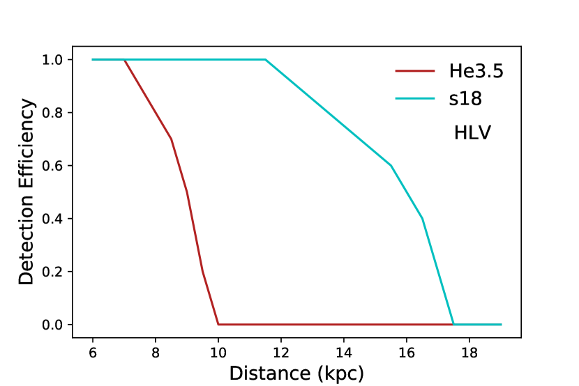
Figure 12: An estimation of the detection distance of models s18 and He3.5 in an Advanced LIGO/Virgo network (left) and the Einstein Telescope detector (right). The maximum detectable distance for model He3.5 is 10 kpc in an Advanced LIGO/Virgo network, and 105 kpc in Einstein Telescope. The maximum detectable distance for model s18 is 17.5 kpc in an Advanced LIGO/Virgo network, and 180 kpc in Einstein Telescope.

The results are shown in Figure 12. In an aLIGO and AdVirgo design sensitivity detector network, we estimate the maximum detectable distance to be 10 kpc for model He3.5, and 17.5 kpc for model s18. The maximum detectable distance in ET data is 105 kpc for model He3.5, and 180 kpc for model s18. This shows that our models are detectable in our Galaxy and beyond the Large Magellanic Cloud with the ET.

We find that our models have larger detection distances than the results in previous detectability studies, which include emission from older neutrino-driven simulations (Gossan et al., 2016; Abbott et al., 2016). CCSN 2D models result in artificially weak gravitational wave energy in the detector due to the single polarization, leading to smaller detection distances. Our new models can be detected at larger distances than the models in Ott et al. (2013) due to our models higher amplitudes and longer durations. The models in Müller et al. (2012) are also of long duration. However, while this model initially also develops strong large-scale convective motions and has similarly strong shock deformation as ours (as exemplified by a tail of similar amplitude), the detection distance of our models are larger. This is because our models exhibit stronger large-scale convective overturn for a longer time after shock revival, whereas accretion downflows are quenched more rapidly in the model of Müller et al. (2012). Previous simulated models with lower peak gravitational wave emission produced by the low-frequency $(\sim 100\,\mathrm{Hz})$ oscillatory SASI motions in the post-shock regions and the PNS surface are likely more detectable in AdVirgo than our models that peak in a higher frequency band where AdVirgo does not have much sensitivity. However, the aLIGO detectors have better sensitivity in the peak frequency range of our models, and ET has better sensitivity across the whole frequency band of all current neutrino-driven CCSN models.

8 Conclusions

In this study, we simulate the explosion of an ultra-stripped star with a helium star mass of $3.5\,M_{\odot}$ and a single star with a ZAMS mass of $18\,M_{\odot}$. We update the neutrino hydrodynamics code CoCoNuT-FMT to include updated neutrino rates and on-the-fly extraction of the gravitational wave emission. We simulate in 3D down to the innermost 10 km to include the PNS convection zone, as this region is essential for accurate gravitational wave emission predictions. To keep the computational costs manageable, we use a reduced number of energy groups than in recent CoCoNuT-FMT models.

Model He3.5 is the first ultra-stripped progenitor simulation to include a calculation of the gravitational wave emission. Understanding ultra-stripped CCSNe is essential as most stars are expected to occur in binary systems. We find our model explodes later than the previous simulation in Müller et al. (2019) due to the lower number of energy groups in our simulation. The model has gravitational wave emission associated with the excitation of g-modes in the PNS with peak frequencies between 800 Hz and 1000 Hz. As none of the properties that determine the frequency of the emission were affected by the lower number of energy groups, we determine that our peak frequencies are still accurate to within a few percent. As the peak gravitational wave amplitude, of $\mathord{\sim}6\,\mathrm{cm}$, occurs after shock revival, our reduced number of energy groups may have resulted in our peak gravitational wave amplitude occurring a little later after core bounce than if a larger number of energy groups were included.

Model s18 reaches even further into the explosion phase as the simulation was stopped 0.9 s after core bounce. There are no significant differences between the explosion dynamics of the model and the previous simulation with a larger number of energy groups. The gravitational wave emission is similar to model He3.5. The emission is due to g-modes oscillations of the PNS, and the frequency peaks between 800 Hz and 1000 Hz. The peak gravitational wave emission begins earlier for this model due to the earlier explosion time, and the larger mass and higher explosion energy of model s18 results in a larger peak gravitation wave amplitude, up to $\sim 10$ cm.

Other recent 3D simulations by Andresen et al. (2017) and Yakunin et al. (2017) have varied wildly in their estimation of the amplitude of their gravitational wave models. We find the amplitude of our models to be closer to those of Andresen et al. (2017), even though our models successfully revive the shock and have greater explosion energy.

We include a discussion of the LESA instabilities observed in our models. We find evidence that the LESA may not be a new instability, but just a manifestation of regular convection. Our analysis highlights the complexity of the LESA and the need for further analysis in future studies to fully understand the effects of the LESA on the gravitational wave emission.

We measure how detectable the gravitational wave emission in our models would be in an aLIGO and AdVirgo design sensitivity detector network, and in the next generation detector ET. We find our larger gravitational wave amplitudes result in detection distances of up to 10 kpc for model He3.5, and up to 17.5 kpc for model s18 in an advanced detector network. In ET, both models are detectable at distances beyond the Large Magellanic Cloud. The detectable distance for our models may improve in the future if more sensitive search techniques for CCSN signals are developed that are sensitive to lower signal-to-noise ratio signals.

Our simulations stop after the peak gravitational wave emission phase and are longer in duration than all of the recent neutrino-driven simulations produced in Andresen et al. (2019); Kuroda et al. (2016); Yakunin et al. (2017); Andresen et al. (2017). This is important for several reasons. The first is that knowledge of the entire gravitational waveform is essential for accurate tuning of gravitational wave searches and parameter estimation algorithms such as those in Powell et al. (2017); Gill et al. (2018); Torres-Forné et al. (2018); Gossan et al. (2016); Abbott et al. (2016). The second is that most of the previous 3D waveforms are produced in simulations that either do not successfully revive the shock, or are stopped too early to reach the shock revival phase. Our models show the peak gravitational wave emission occurs after shock revival, therefore some previous neutrino-driven simulations may have ended before their peak gravitational wave emission occurred. The frequency of the emission produced in g-mode oscillations increases with time, which may explain why our models have a higher peak gravitational wave frequency than previous work with shorter end times.

References

- Abbott et al. (2016) Abbott B. P., et al., 2016, Phys. Rev. D, 94, 102001
- Abbott et al. (2018) Abbott B. P., et al., 2018, Living Reviews in Relativity, 21, 3
- Abdikamalov et al. (2014) Abdikamalov E., Gossan S., DeMaio A. M., Ott C. D., 2014, Phys. Rev. D, 90, 044001
- Acernese & et al. (2015) Acernese F., et al. 2015, Classical and Quantum Gravity, 32, 024001
- Andresen et al. (2017) Andresen H., Müller B., Müller E., Janka H.-T., 2017, MNRAS, 468, 2032
- Andresen et al. (2019) Andresen H., Müller E., Janka H. T., Summa A., Gill K., Zanolin M., 2019, MNRAS, 486, 2238
- Ashton et al. (2019) Ashton G., et al., 2019, ApJS, 241
- Beck et al. (2012) Beck P. G., et al., 2012, Nature, 481, 55
- Blondin & Mezzacappa (2006) Blondin J. M., Mezzacappa A., 2006, ApJ, 642, 401
- Blondin et al. (2003) Blondin J. M., Mezzacappa A., DeMarino C., 2003, The Astrophysical Journal, 584, 971
- Bollig et al. (2017) Bollig R., Janka H.-T., Lohs A., Martínez-Pinedo G., Horowitz C. J., Melson T., 2017, Physical Review Letters, 119, 242702
- Bruenn & Dineva (1996) Bruenn S. W., Dineva T., 1996, ApJ, 458, L71
- Bruenn et al. (2004) Bruenn S. W., Raley E. A., Mezzacappa A., 2004, ArXiv Astrophysics e-prints,
- Buras et al. (2006a) Buras R., Rampp M., Janka H.-T., Kifonidis K., 2006a, A&A, 447, 1049
- Buras et al. (2006b) Buras R., Janka H.-T., Rampp M., Kifonidis K., 2006b, A&A, 457, 281
- Burrows (2013) Burrows A., 2013, Reviews of Modern Physics, 85, 245
- Burrows et al. (1995) Burrows A., Hayes J., Fryxell B. A., 1995, ApJ, 450, 830
- Cerdá-Durán et al. (2013) Cerdá-Durán P., DeBrye N., Aloy M. A., Font J. A., Obergaulinger M., 2013, ApJ, 779, L18
- Chini et al. (2012) Chini R., Hoffmeister V. H., Nasseri A., Stahl O., Zinnecker H., 2012, MNRAS, 424, 1925
- Dessart et al. (2006) Dessart L., Burrows A., Livne E., Ott C. D., 2006, ApJ, 645, 534
- Dimmelmeier et al. (2002) Dimmelmeier H., Font J. A., Müller E., 2002, A&A, 393, 523
- Dimmelmeier et al. (2008) Dimmelmeier H., Ott C. D., Marek A., Janka H.-T., 2008, Phys. Rev. D, 78, 064056
- Fischer et al. (2018) Fischer T., Martínez-Pinedo G., Wu M.-R., Lohs A., Qian Y.-Z., 2018, preprint, (arXiv:1804.10890)
- Foglizzo et al. (2007) Foglizzo T., Galletti P., Scheck L., Janka H.-T., 2007, ApJ, 654, 1006
- Fuller et al. (2015) Fuller J., Klion H., Abdikamalov E., Ott C. D., 2015, MNRAS, 450, 414
- Gill et al. (2018) Gill K., Wang W., Valdez O., Szczepanczyk M., Zanolin M., Mukherjee S., 2018, preprint, (arXiv:1802.07255)
- Glas et al. (2018) Glas R., Janka H.-T., Melson T., Stockinger G., Just O., 2018, preprint, (arXiv:1809.10150)
- Goldreich & Kumar (1990) Goldreich P., Kumar P., 1990, ApJ, 363, 694
- Gossan et al. (2016) Gossan S. E., Sutton P., Stuver A., Zanolin M., Gill K., Ott C. D., 2016, Phys. Rev. D, 93, 042002
- Herant et al. (1994) Herant M., Benz W., Hix W. R., Fryer C. L., Colgate S. A., 1994, ApJ, 435, 339
- Hild et al. (2008) Hild S., Chelkowski S., Freise A., 2008, preprint, (arXiv:0810.0604)
- Hobbs et al. (2016) Hobbs T. J., Alberg M., Miller G. A., 2016, Phys. Rev. C, 93, 052801
- Horowitz (2002) Horowitz C. J., 2002, Phys. Rev. D, 65, 043001
- Horowitz et al. (2017) Horowitz C. J., Caballero O. L., Lin Z., O’Connor E., Schwenk A., 2017, Phys. Rev. C, 95, 025801
- Janka (2012) Janka H.-T., 2012, Annual Review of Nuclear and Particle Science, 62, 407
- Janka & Müller (1995) Janka H.-T., Müller E., 1995, ApJ, 448, L109
- Just et al. (2018) Just O., Bollig R., Janka H.-T., Obergaulinger M., Glas R., Nagataki S., 2018, MNRAS, 481, 4786
- Keil et al. (1996) Keil W., Janka H.-T., Mueller E., 1996, ApJ, 473, L111
- Kotake (2013) Kotake K., 2013, Comptes Rendus Physique, 14, 318
- Kotake & Kuroda (2017) Kotake K., Kuroda T., 2017, in Alsabti A. W., Murdin P., eds, , Handbook of Supernovae. pringer International Publishing AG, p. 1671, doi:10.1007/978-3-319-21846-5_9
- Kumar et al. (2014) Kumar A., Chatterjee A. G., Verma M. K., 2014, Phys. Rev. E, 90, 023016
- Kuroda et al. (2016) Kuroda T., Kotake K., Takiwaki T., 2016, ApJ, 829, L14
- Lattimer & Mazurek (1981) Lattimer J. M., Mazurek T. J., 1981, ApJ, 246, 955
- Lattimer & Swesty (1991) Lattimer J. M., Swesty F. D., 1991, Nucl. Phys., A535, 331
- Lynch et al. (2017) Lynch R., Vitale S., Essick R., Katsavounidis E., Robinet F., 2017, Phys. Rev. D, 95, 104046
- Marek (2007) Marek A., 2007, PhD thesis, Technische Universtiät München
- Martínez-Pinedo et al. (2012) Martínez-Pinedo G., Fischer T., Lohs A., Huther L., 2012, Physical Review Letters, 109, 251104
- Melson et al. (2015) Melson T., Janka H.-T., Bollig R., Hanke F., Marek A., Müller B., 2015, ApJ, 808, L42
- Mirizzi et al. (2016) Mirizzi A., Tamborra I., Janka H.-T., Saviano N., Scholberg K., Bollig R., Hüdepohl L., Chakraborty S., 2016, Nuovo Cimento Rivista Serie, 39, 1
- Morozova et al. (2018) Morozova V., Radice D., Burrows A., Vartanyan D., 2018, ApJ, 861, 10
- Mosser et al. (2012) Mosser B., et al., 2012, A&A, 548, A10
- Mueller & Janka (1997) Mueller E., Janka H.-T., 1997, A&A, 317, 140
- Müller (2015) Müller B., 2015, MNRAS, 453, 287
- Müller (2017) Müller B., 2017, arXiv e-prints,
- Müller & Janka (2014) Müller B., Janka H.-T., 2014, ApJ, 788, 82
- Müller & Janka (2015) Müller B., Janka H.-T., 2015, MNRAS, 448, 2141
- Müller et al. (2010) Müller B., Janka H.-T., Dimmelmeier H., 2010, ApJS, 189, 104
- Müller et al. (2012) Müller E., Janka H.-T., Wongwathanarat A., 2012, A&A, 537, A63
- Müller et al. (2013) Müller B., Janka H.-T., Marek A., 2013, ApJ, 766, 43
- Müller et al. (2016) Müller B., Viallet M., Heger A., Janka H.-T., 2016, ApJ, 833, 124
- Müller et al. (2017) Müller B., Melson T., Heger A., Janka H.-T., 2017, MNRAS, 472, 491
- Müller et al. (2019) Müller B., et al., 2019, MNRAS, 484, 3307
- Murphy et al. (2009) Murphy J. W., Ott C. D., Burrows A., 2009, ApJ, 707, 1173
- Murphy et al. (2013) Murphy J. W., Dolence J. C., Burrows A., 2013, ApJ, 771, 52
- O’Connor & Couch (2018) O’Connor E. P., Couch S. M., 2018, ApJ, 865, 81
- Obukhov (1959) Obukhov A. M., 1959, Dokl.~Akad.~Nauk SSSR, 125, 124
- Ott et al. (2013) Ott C. D., et al., 2013, ApJ, 768, 115
- Powell et al. (2016) Powell J., Gossan S. E., Logue J., Heng I. S., 2016, Phys. Rev. D, 94, 123012
- Powell et al. (2017) Powell J., Szczepanczyk M., Heng I. S., 2017, Phys. Rev. D, 96, 123013
- Punturo et al. (2010) Punturo M., et al., 2010, Classical and Quantum Gravity, 27, 194002
- Radice et al. (2018) Radice D., Morozova V., Burrows A., Vartanyan D., Nagakura H., 2018, arXiv e-prints,
- Rampp & Janka (2002) Rampp M., Janka H.-T., 2002, A&A, 396, 361
- Richers et al. (2017) Richers S., Ott C. D., Abdikamalov E., O’Connor E., Sullivan C., 2017, Phys. Rev. D, 95, 063019
- Sana et al. (2013) Sana H., et al., 2013, in Pugliese G., de Koter A., Wijburg M., eds, Astronomical Society of the Pacific Conference Series Vol. 470, 370 Years of Astronomy in Utrecht. p. 141 (arXiv:1211.4740)
- Scheidegger et al. (2010) Scheidegger S., Käppeli R., Whitehouse S. C., Fischer T., Liebendörfer M., 2010, A&A, 514, A51
- Smith & Thrane (2018) Smith R., Thrane E., 2018, Physical Review X, 8, 021019
- Takiwaki & Kotake (2018) Takiwaki T., Kotake K., 2018, MNRAS, 475, L91
- Tamborra et al. (2014) Tamborra I., Hanke F., Janka H.-T., Müller B., Raffelt G. G., Marek A., 2014, ApJ, 792, 96
- Tauris et al. (2013) Tauris T. M., Langer N., Moriya T. J., Podsiadlowski P., Yoon S. C., Blinnikov S. I., 2013, ApJ, 778, L23
- Tauris et al. (2015) Tauris T. M., Langer N., Podsiadlowski P., 2015, MNRAS, 451, 2123
- The LIGO Scientific Collaboration et al. (2015) The LIGO Scientific Collaboration Aasi J., Abbott B. P., Abbott R., et al. 2015, Classical and Quantum Gravity, 32, 074001
- Torres-Forné et al. (2018) Torres-Forné A., Cerdá-Durán P., Passamonti A., Font J. A., 2018, MNRAS, 474, 5272
- Wellstein et al. (2001) Wellstein S., Langer N., Braun H., 2001, A&A, 369, 939
- Yakunin et al. (2010) Yakunin K. N., et al., 2010, Classical and Quantum Gravity, 27, 194005
- Yakunin et al. (2015) Yakunin K. N., et al., 2015, Phys. Rev. D, 92, 084040
- Yakunin et al. (2017) Yakunin K. N., et al., 2017, preprint, (arXiv:1701.07325)