On the sign recovery by LASSO, thresholded LASSO and thresholded Basis Pursuit Denoising

Abstract

Basis Pursuit (BP), Basis Pursuit DeNoising (BPDN), and LASSO are popular methods for identifying important predictors in the high-dimensional linear regression model $Y=X\beta+\varepsilon$. By definition, when $\varepsilon=0$, BP uniquely recovers $\beta$ when $X\beta=Xb$ and $\beta\neq b$ implies $\|b\|_{1}>\|\beta\|_{1}$ (identifiability condition). Furthermore, LASSO can recover the sign of $\beta$ only under a much stronger irrepresentability condition. Meanwhile, it is known that the model selection properties of LASSO can be improved by hard-thresholding its estimates. This article supports these findings by proving that thresholded LASSO, thresholded BPDN and thresholded BP recover the sign of $\beta$ in both the noisy and noiseless cases if and only if $\beta$ is identifiable and large enough. In particular, if $X$ has iid Gaussian entries and the number of predictors grows linearly with the sample size, then these thresholded estimators can recover the sign of $\beta$ when the signal sparsity is asymptotically below the Donoho-Tanner transition curve. This is in contrast to the regular LASSO, which asymptotically, recovers the sign of $\beta$ only when the signal sparsity tends to 0. Numerical experiments show that the identifiability condition, unlike the irrepresentability condition, does not seem to be affected by the structure of the correlations in the $X$ matrix.

Keywords: Multiple regression, Basis Pursuit, LASSO, Sparsity, Active set estimation, Sign estimation, Identifiability condition, Irrepresentability condition

1 Introduction

Let us consider the high dimensional linear model

$$Y=X\beta+\varepsilon,$$ (1)

where $X=(X_{1}|\dots|X_{p})$ is a $n\times p$ design matrix with $n\leq p$, $\varepsilon$ is a random vector in $\mathbb{R}^{n}$, and $\beta\in\mathbb{R}^{p}$ is an unknown vector of regression coefficients. The sign vector of $\beta$ is $S(\beta)=(S(\beta_{1}),\dots S(\beta_{p}))\in\{-1,0,1\}^{p}$, where for $x\in\mathbb{R}$, $S(x)={\bf 1}_{x>0}-{\bf 1}_{x<0}$. Our main goal is to recover $S(\beta)$. This goal is somewhat more general than the goal of recovering the active set, ${\rm supp}(\beta):=\{i\in\{1,\dots,p\}\mid\beta_{i}\neq 0\}$. Indeed, given $S(\beta)$ one may recover ${\rm supp}(\beta)$ since ${\rm supp}(\beta):=\{i\in\{1,\dots,p\}\mid S(\beta_{i})\neq 0\}$ but conversely, given ${\rm supp}(\beta)$, one cannot recover $S(\beta)$. Moreover, some theoretical works recommend sign recovery instead of active set recovery [17, 27].

1.1 BP, BPDN and LASSO

First introduced in signal processing [7], BP estimator is a solution of the following optimization problem

$$\hat{\beta}^{\rm BP}:={\text{\rm argmin }}\|b\|_{1}\;\;\text{\rm subject to }Y=Xb,$$

which can be solved using linear programming. In the noiseless case, when $\varepsilon=0$ and $Y=X\beta$, we say that $\beta$ is identifiable with respect to $X$ and the $\ell_{1}$ norm if $\hat{\beta}^{\rm BP}$ uniquely recovers $\beta$ i.e. if $b\neq\beta$, $Xb=X\beta$ implies $\|b\|_{1}>\|\beta\|_{1}$. Note that a geometric characterization of the identifiability condition, depending on $X$ and the sign of $\beta$, is given in [26]. This condition implies that $\beta$ is sparse. Indeed, Lemma 3 in Tardivel et al. [30] shows that ${\rm card}\{i\in\{1,\dots,p\}\mid\hat{\beta}^{\rm BP}_{i}\neq 0\}\leq n$ i.e. $\hat{\beta}^{\rm BP}$ has at least $p-n$ zeros. Consequently having $k\leq n$, where $k$ is the number of non-zero elements in $\beta$, is necessary for the identifiability condition. On the other hand, some assumptions on the sparsity of $\beta$ guarantee that $\beta$ is identifiable with respect to the $\ell_{1}$ norm. For example, the identifiability condition holds if the number of non-zero elements of $\beta$ satisfies the mutual coherence condition [12, 16, 19]. In the special case where the elements of $X$ are iid normal variables, the transition curve $\rho:(0,1)\mapsto(0,1)$ [11] characterizes the identifiability condition with respect to the signal sparsity $\xi=k/n$. In particular, it is known that the identifiability condition is satisfied with probability converging to 1 if $\xi<\rho(\delta)$ or converging to 0 if $\xi>\rho(\delta)$.

In the case where $\varepsilon$ has a continuous distribution, almost surely BP has $n$ non-zero components and thus BP cannot recover the sign of $\beta$ once $k\neq n$. To account for noise, when $\varepsilon$ has iid $\mathcal{N}(0,\sigma^{2})$ entries for some $\sigma>0$, Chen and Donoho [7] extended BP by proposing the following estimation algorithm:

$$\widehat{\beta}^{\rm L}:=\underset{b\in\mathbb{R}^{p}}{\text{\rm argmin }}\frac{1}{2}\|Y-Xb\|_{2}^{2}+\lambda\|b\|_{1}\text{ \rm with }\lambda=\sigma\sqrt{2\log p}.$$ (2)

In the seminal work of Tibshirani [31], the algorithm was extended for fitting the general multiple regression models where different values of $\lambda$ are often more appropriate. The method gained great popularity in the statistical community under the name LASSO (Least Absolute Shrinkage and Selection Operator), while in the signal processing community it is often called Basis Pursuit Denoising (BPDN). In this paper, we will use the term BPDN for a slightly different form of this estimator, where association with BP is even clearer

$$\widehat{\beta}^{\rm BPDN}:=\underset{b\in\mathbb{R}^{p}}{\text{\rm argmin }}\|b\|_{1}\;\text{\rm subject to }\|Y-Xb\|_{2}^{2}\leq R,\text{\rm where }R\geq 0.$$ (3)

Note that $X$ is fixed but $Y$ is random, and that for a given $\lambda>0$ for LASSO we cannot choose a fixed $R>0$ for BPDN under which the two estimators are almost surely equal. To illustrate this fact, we note that $\widehat{\beta}^{\rm BPDN}=0$ if and only if $\|Y\|_{2}^{2}\leq R$, while for LASSO $\widehat{\beta}^{\rm L}=0$ if and only if $\|X^{\prime}Y\|_{\infty}\leq\lambda$.

1.2 Sign recovery by LASSO

Properties of the LASSO sign estimator $S(\widehat{\beta}^{\rm L}(\lambda)):=\left(S(\widehat{\beta}^{\rm L}_{1}(\lambda)),\dots,S(\widehat{\beta}^{\rm L}_{p}(\lambda))\right)$ (or properties of the active set estimator ${\rm supp}(\widehat{\beta}^{\rm L}(\lambda)):=\{i\in\{1,\dots,p\}\mid\widehat{\beta}^{\rm L}_{i}(\lambda)\neq 0\}$) have been intensively studied [14, 21, 22, 35, 39, 40]. According to Theorem 2 of Wainwright [35], the irrepresentability condition is necessary for LASSO to recover $S(\beta)$ with high probability. Indeed, if $\ker(X_{I})=\{{\bf 0}\}$, $\|X_{\overline{I}}^{\prime}X_{I}(X_{I}^{\prime}X_{I})^{-1}S(\beta_{I})\|_{\infty}>1$ and both $\varepsilon$ and $-\varepsilon$ have the same distribution, then for any choice of the tuning parameter $\lambda>0$, $\mathbb{P}(S(\widehat{\beta}^{\rm L}(\lambda))=S(\beta))\leq 1/2$. This result also holds for the noiseless case, in which LASSO does not recover $S(\beta)$. Moreover, Bühlmann and van de Geer [4] (pp. 192-194) have shown that if $\varepsilon={\bf 0}$ and the irrepresentability holds strictly (i.e., if $\|X_{\overline{I}}^{\prime}X_{I}(X_{I}^{\prime}X_{I})^{-1}S(\beta_{I})\|_{\infty}<1$) then the nonrandom set ${\rm supp}(\widehat{\beta}^{L}(\lambda))$ is equal to ${\rm supp}(\beta)$ as long as the non-zero components of $\beta$ are sufficiently large. The proof given in [4] can be easily adapted for sign recovery.

Proposition 1, proved in the Appendix, shows that the identifiability condition is weaker than the irrepresentability condition.

Proposition 1

Let $X$ be an $n\times p$ matrix with $p\geq n$ columns in general position. Moreover, let $\beta\in\mathbb{R}^{p}$, $I:={\rm supp}(\beta)$ and suppose that $\ker(X_{I})=\{{\bf 0}\}$. If the irrepresentability condition holds, then the parameter $\beta$ is identifiable with respect to the $\ell_{1}$norm.

For the case where the elements of $X$ are iid random variables from the normal distribution, the irrepresentability condition is satisfied with high probability if and only if $k<\frac{n}{2\log p}$ (see [35]). This implies that LASSO cannot recover $S(\beta)$ when $k/n\to\xi>0$, even if $\xi<\rho(\delta)$.

1.3 Sign recovery by thresholded LASSO

It is well known that LASSO can consistently estimate $\beta$ under much weaker assumptions than the irrepresentability condition (see, e.g., [23] or [34]). This suggests that an appropriately thresholded version of LASSO can recover $S(\beta)$ under weaker assumptions than the irrepresentability condition [24]. Concerning sign recovery by thresholded BP, first theoretical results were given by Saligrama and Zhao [25]. More recently, Descloux and Sardy [9] show that the stable null space property is a sufficient condition to recover the sign of $\beta$ by thresholded BP.

To our knowledge, the stable null space property has so far been the weakest sufficient condition known to guarantee the recovery of $S(\beta)$. In Theorem 1, we show that “identifiability”, a weaker condition than the stable null space property, is sufficient to recover $S(\beta)$ by thresholded BP, thresholded BPDN or thresholded LASSO when the non-zero elements of $\beta$ are large enough. We also show that “identifiability” is a necessary condition for the recovery of $S(\beta)$ by these methods, regardless of the signal magnitude.

Theorem 1 implies that in the linear sparsity regime of [11] for Gaussian matrices, thresholded BP, thresholded BPDN and thresholded LASSO recover $S(\beta)$ if, asymptotically, $k<n\rho(n/p)$ holds and the signal magnitude tends towards infinity. Table 1 summarizes known conditions for sign or support recovery by LASSO and related methods, when $\varepsilon\neq 0$ and the signal is large enough.

Method	Conditions	Type	Related articles
Regular	Mutual coherence	sufficient	[6, 21]
LASSO	Irrepresentability	necessary and sufficient	[14, 22, 35, 39, 40]
Thresholded	Stable null space	sufficient	[9]
LASSO, BP	Identifiability	necessary and sufficient	current article

Table 1: Some theoretical conditions under which LASSO and related methods can recover the sign or the support of $\beta$ when $\varepsilon\neq 0$ and non-zero elements of $\beta$ are large enough. Additional comments related to these conditions are given in Appendix.

1.4 Graphical illustration of the main result

By definition, the irrepresentability condition depends on $\beta$ by $S(\beta)$. Moreover, as asserted in Proposition 2, the identifiability condition similarly depends only on $S(\beta)$. Thus, the comparison of these two conditions can be performed by considering parameter vectors such that $\beta=S(\beta)$. In Figure 1, we plot the irrepresentability and identifiability curves representing the proportion of sign vectors for which the identifiability condition or the irrepresentability condition is satisfied among $k-$sparse sign vectors. For each value of $k$, this proportion was estimated by generating 1000 sign vectors from a uniform distribution on the set $\{u\in\{-1,0,1\}^{p}\mid{\rm card}({\rm supp}(u))=k\}$.

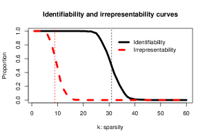
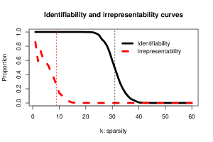
Figure 1: Simulated identifiability and irrepresentability curves for two specific design matrices of dimensions $100\times 300$. In both cases the rows of $X$ were generated as iid random vectors from the multivariate normal distribution $N(0,\Sigma)$, with $\Sigma=I$ in the left panel and $\Sigma$ in the second panel having a compound symmetry form with $\Sigma_{ii}=1$ and $\Sigma_{ij}=0.9$ for $i\neq j$. The x-axis represents the sparsity $k$ and the y-axis the fraction of sign vectors that satisfy the identifiability condition (respectively, irrepresentability condition). In the left panel, the vertical lines represent the values $k=\frac{100}{2\log(300)}$ and $k=100\times\rho(100/300)$. These values correspond to the asymptotic upper bounds for $k$ so the irrepresentability and identifiability conditions hold for Gaussian design matrices with independent entries.

Figure 1 shows a large potential for improvement in sign detection by thresholded LASSO compared to the base LASSO. If the columns of the design matrix are independent Gaussian vectors, then the irrepresentability condition is satisfied with high probability only if $k\leq 10$, which is also a limiting sparsity for the recovery of $S(\beta)$ by LASSO. Instead, the identifiability condition, which provides the limiting sparsity for the recovery of $S(\beta)$ by the thresholded LASSO, holds as long as $k\leq 30$. The simulations are in strong agreement with the asymptotic results in [35] and [13], which predict the upper bounds for $k$ such that the irrepresentability and identifiability conditions hold for Gaussian design matrices with independent entries.

The difference between identifiability and irrepresentability curves becomes even more apparent when there are strong correlations between different columns in the design matrix. As expected, the irrepresentability curve shrinks towards zero. Instead, and rather unexpectedly, the simulated identifiability curve remains intact.

1.5 Organization of the article

In Section 2, Theorem 1 shows that identifiability is a necessary and sufficient condition for LASSO to separate the non-zero components of $\beta$ from the noise and to recover asymptotically $S(\beta)$ with thresholded LASSO and thresholded BPDN. Corollary 1 shows that under the asymptotic linear sparsity regime for Gaussian matrices thresholded LASSO and thresholded BPDN can recover the sign of $\beta$ when asymptotically $k<n\rho(n/p)$.

In Section 3, Proposition 2 shows that the identifiability condition depends only on $S(\beta)$ and not on the size of the non-zero components of $\beta$. Here we also introduce the irrepresentability and identifiability curves, which respectively give the fraction of $k-$sparse sign vectors satisfying the irrepresentability condition and the identifiability condition. Section 4 is devoted to numerical experiments showing that sign estimators derived from the thresholded LASSO and the thresholded BPDN are better than sign estimators derived from LASSO and the adaptive LASSO, and that the knockoff method allows appropriate threshold selection for both methods. The proofs are in the Appendix. In this section, we also formulate Proposition 3 providing a tight upper bound on the probability of recovering $S(\beta)$ through LASSO.

1.6 Notation and assumptions

In this article we always assume that the design matrix $X$ has columns in general position (see, e.g., [32] or the supplementary material for this manuscript). This assumption guarantees that the minimizer of (2) (resp. minimizer of (3)) is unique and that therefore the LASSO estimator (resp. BPDN estimator) is well-defined. This assumption is very weak and generically holds. Indeed, when $X$ is a random matrix such that the entries $(X_{11},X_{12},\dots,X_{np})$ have a density on $\mathbb{R}^{np}$ then, almost surely, $X$ is in general position [32].

Notation used in the following sections is as follows:

• Let $I$ be a subset of $\{1,\dots,p\}$. We denote by $\overline{I}$ the complement of $I$, namely $\overline{I}:=\{1,\dots,p\}\setminus I$.

• The notation $X_{I}$ stands for a matrix whose columns are indexed by the elements of $I$: $(X_{i})_{i\in I}$.

• For $b\in\mathbb{R}^{p}$, $b_{I}$ denotes the subvector containing elements of $b$ with indices in $I$.

• The symbols ${\rm supp}(b),{\rm supp}^{+}(b)$ and ${\rm supp}^{-}(b)$ denote, respectively, the sets $\{i\in\{1,\dots,p\}\mid b_{i}\neq 0\},\{i\in\{1,\dots,p\}\mid b_{i}>0\}$ and $\{i\in\{1,\dots,p\}\mid b_{i}<0\}$.

• LASSO and BPDN estimators depend on $X,\beta,\varepsilon$ and the tuning parameter $\lambda>0$ or the regularization parameter $R\geq 0$. When appropriate, we use the parentheses to indicate these dependencies. The estimator $\widehat{\beta}$ indiscriminately represents the LASSO estimator or the BPDN estimator.

To formulate our asymptotic results, we will often consider a sequence of regression parameters $\beta^{(r)}\in\mathbb{R}^{p}$, $r\in\mathbb{N}$, for which non-zero components tend to infinity in the following way.

Assumption 1

 

• The sign of $\beta^{(r)}$ is invariant, namely there exists a sign vector $s^{0}\in\{-1,0,1\}^{p}$ such that for any $r\in\mathbb{N},S(\beta^{(r)})=s^{0}$.

• The following limit holds $\lim_{r\to+\infty}\min\{|\beta^{(r)}_{i}|,i\in{\rm supp}(s^{0})\}=+\infty$.

• There exists $q>0$ such that

  $$\forall r\in\mathbb{N},\frac{\min\{|\beta^{(r)}_{i}|,i\in{\rm supp}(s^{0})\}}{\|\beta^{(r)}\|_{\infty}}\geq q.$$

2 Identifiability is a necessary and sufficient condition for the sign recovery

If $\beta$ does not satisfy the irrepresentability condition, then the LASSO sign estimator $S(\widehat{\beta}^{\rm L}(\lambda))$ is very unlikely to recover $S(\beta)$. However, one may relax this condition. In fact, Theorem 1 shows that an appropriately thresholded version of LASSO (or thresholded version of BPDN) recovers $S(\beta)$ if only the non-zero elements of $\beta$ are sufficiently large and the identifiability condition is satisfied.

Theorem 1

Let $X$ be a $n\times p$ matrix in general position and such that ${\rm rank}(X)=n$ and let $\widehat{\beta}$ be the LASSO or BPDN estimator with any fixed value of the tuning parameter $\lambda>0$ or with any fixed regularization parameter $R\geq 0$.
Necessary condition for sign recovery: If $S(\beta)$ is unidentifiable with respect to the $\ell_{1}$ norm, then the sign estimator derived from the thresholded LASSO or thresholded BPDN cannot recover $S(\beta)$. Indeed, for each fixed $\varepsilon\in\mathbb{R}^{n}$, the sign of at least one non-zero component of $\beta$ is not correctly estimated by $\widehat{\beta}(\varepsilon)$:

$$\exists i\in{\rm supp}(\beta)\text{ \rm such that }\widehat{\beta}_{i}(\varepsilon)\beta_{i}\leq 0.$$

Sufficient condition for sign recovery: Let $\beta^{(r)}$ be a sequence in $\mathbb{R}^{p}$ satisfying Assumption 1. If $s^{0}$ is identifiable with respect to the $\ell_{1}$ norm, then for any fixed $\varepsilon\in\mathbb{R}^{n}$ and sufficiently large $r>r_{0}(\varepsilon)$ the estimator $\widehat{\beta}(\varepsilon,r)$ separates negative components of $\beta^{(r)}$ (i.e $i\in{\rm supp}^{-}(\beta^{(r)})$), zero components of $\beta^{(r)}$ (i.e $i\notin{\rm supp}(\beta^{(r)})$) and positive components of $\beta^{(r)}$ (i.e $i\in{\rm supp}^{+}(\beta^{(r)})$):

• $$\forall i\in{\rm supp}(\beta^{(r)}),\,\,\widehat{\beta}_{i}(\varepsilon,r)\beta^{(r)}_{i}>0.$$

• $$\max_{i\in{\rm supp}^{-}(\beta^{(r)})}\left\{\widehat{\beta}_{i}(\varepsilon,r)\right\}<\min_{i\notin{\rm supp}(\beta^{(r)})}\left\{\widehat{\beta}_{i}(\varepsilon,r)\right\}\leq\max_{i\notin{\rm supp}(\beta^{(r)})}\left\{\widehat{\beta}_{i}(\varepsilon,r)\right\}<\min_{i\in{\rm supp}^{+}(\beta^{(r)})}\left\{\widehat{\beta}_{i}(\varepsilon,r)\right\}.$$

Let us note that the assumptions about $X$ are very weak and hold in general if $n\leq p$. The assumption that ${\rm rank}(X)=n$ ensures that the BPDN estimator is well-defined for any $R\geq 0$. The general position condition ensures uniqueness of both the LASSO and the BPDN estimator (see, e.g., Proposition 1 in the Supplementary Material).

Theorem 1 emphasises that one cannot recover $S(\beta)$ with a sign estimator derived from LASSO or BPDN if $\beta$ is not identifiable with respect to the $\ell_{1}$ norm. If $\beta$ is identifiable with respect to the $\ell_{1}$norm, Theorem 1 implies that $S(\beta)$ can be recovered by deriving sign estimators from the thresholded LASSO or thresholded BPDN. In Section 4, we show how the appropriate thresholds can be obtained using control variables constructed by the knockoff method (see, e.g., [1, 5]).

In the asymptotic linear sparsity regime for Gaussian matrices, the transition curve $\rho(\cdot)$ described in [11] allows us to characterize the identifiability condition, and so Theorem 1 yields the Corollary 1.

Corollary 1

Let $X$ be a $n\times p_{n}$ standard Gaussian matrix and let $k_{n}$ denote the number of non-zero components of $\beta^{(n)}\in\mathbb{R}^{p_{n}}$.
Necessary condition for sign recovery: If $n/p_{n}\rightarrow\delta\in(0,1)$, $k_{n}/n\rightarrow\xi\in(0,1)$ and $\xi>\rho(\delta)$ then asymptotically the sign of at least one non-zero component of $\beta^{(n)}$ is incorrectly estimated by $\widehat{\beta}$:

$$\lim_{n\to+\infty}\mathbb{P}_{X,\varepsilon}\left(\exists i\in{\rm supp}(\beta^{(n)})\text{ \rm such that }\widehat{\beta}_{i}\beta^{(n)}_{i}\leq 0\right)=1.$$

Sufficient condition for sign recovery: Given $n$, let $(\beta^{(n,r)})_{r\in\mathbb{N}}$ be a sequence satisfying the Assumption 1 (where $q$ does not depend on $n$). If $n/p_{n}\rightarrow\delta\in(0,1)$, $k_{n}/n\rightarrow\xi\in(0,1)$ and $\xi<\rho(\delta)$ then the estimator $\widehat{\beta}$ asymptotically separates the negative components of $\beta^{(n,r)}$, zero components of $\beta^{(n,r)}$ and positive components of $\beta^{(n,r)}$:

• $$\lim_{n\to+\infty}\lim_{r\to+\infty}\mathbb{P}_{X,\varepsilon}\left(\forall i\in{\rm supp}(\beta^{(n,r)}),\,\,\widehat{\beta}_{i}\beta^{(n,r)}_{i}>0\right)=1.$$

• $$\lim_{n\to+\infty}\lim_{r\to+\infty}\mathbb{P}_{X,\varepsilon}\left(\max_{i\in{\rm supp}^{-}(\beta^{(n,r)})}\left\{\widehat{\beta}_{i}\right\}<\min_{i\notin{\rm supp}(\beta^{(n,r)})}\left\{\widehat{\beta}_{i}\right\}\leq\max_{i\notin{\rm supp}(\beta^{(n,r)})}\left\{\widehat{\beta}_{i}\right\}<\min_{i\in{\rm supp}^{+}(\beta^{(n,r)})}\left\{\widehat{\beta}_{i}\right\}\right)=1.$$

3 Identifiability and irrepresentability curves

Given a certain design matrix $X$, we now define the irrepresentability indicator of the sign vector $s$.
Sign irrepresentability indicator:

$$\Phi^{X}_{\rm IC}:s\in\{-1,0,1\}^{p}\mapsto\begin{cases}1\text{ \rm if }s=(0,\dots,0)\\ 1\text{ \rm if }\ker(X_{I})=\{{\bf 0}\}\text{ \rm and }\|X_{\overline{I}}^{\prime}X_{I}(X_{I}^{\prime}X_{I})^{-1}s_{I}\|_{\infty}\leq 1\text{ \rm where }I:={\rm supp}(s)\\ 0\text{ \rm otherwise }\end{cases}.$$

This irrepresentability indicator shows whether the LASSO sign estimator can recover $S(\beta)$. Namely, if $\phi^{X}_{\rm IC}(S(\beta))=0$ then $S(\beta)$ cannot be recovered using the LASSO sign estimator, even if the non-zero components of $\beta$ are extremely large.

Proposition 2 shows that the identifiability condition also depends only on $S(\beta)$ and not on the sizes of the non-zero components of $\beta$.

Proposition 2

Consider two vectors $b\in\mathbb{R}^{p}$ and $\tilde{b}\in\mathbb{R}^{p}$ such that $S(b)=S(\tilde{b})$. Then $\tilde{b}$ is identifiable with respect to the matrix $X$ and the $\ell_{1}$ norm if and only if $b$ is identifiable with respect to the matrix $X$ and the $\ell_{1}$ norm.

Given a certain design matrix $X$, the sign identifiability indicator is defined as follows.
Sign identifiability indicator:

$$\Phi^{X}_{\rm Idtf}:s\in\{-1,0,1\}^{p}\mapsto\begin{cases}0\text{ \rm if }s\neq\underset{b\in\mathbb{R}^{p}}{\text{ \rm argmin }}\|b\|_{1}\text{ \rm subject to }Xb=Xs\\ 1\text{ \rm otherwise }\end{cases}.$$

This identifiability indicator shows whether the sign estimators obtained by thresholded LASSO and thresholded BPDN can recover $S(\beta)$. Namely, if $\phi^{X}_{\rm Idtf}(S(\beta))=0$ then the thresholded LASSO (respectively, thresholded BPDN) sign estimator fails to recover $S(\beta)$ even if the non-zero components of $\beta$ are extremely large.

According to Proposition 2 in the Supplementary Material, $\beta$ does not satisfy the identifiability condition if the columns $(X_{i})_{i\in{\rm supp}(\beta)}$ are not linearly independent. Consequently, if ${\rm card}({\rm supp}(\beta))>n$ then $\phi^{X}_{\rm IC}(S(\beta))=\phi^{X}_{\rm Idtf}(S(\beta))=0$. Let us give some basic properties and comments about the two indicator functions.

1. Both $\phi^{X}_{\rm IC}$ and $\phi^{X}_{\rm Idtf}$ are even.

2. Given Proposition 1, for each $s\in\{-1,0,1\}^{p}$, $\Phi^{X}_{\rm IC}(s)\leq\Phi^{X}_{\rm Idtf}(s)$.

3. The computation of $\Phi^{X}_{\rm IC}$ requires only a simple matrix calculus; the computation of $\Phi^{X}_{\rm Idtf}$ requires only solving the basis pursuit problem.

3.1 Graphs of identifiability and irrepresentability curves

The number of sign vectors is very large ($3^{p}$) and therefore we cannot explicitly specify $\Phi^{X}_{\rm Idtf}$ and $\Phi^{X}_{IC}$ for each sign vector. Instead, we define the identifiability and irrepresentability curves as the following functions of the sparsity $k$ of the vector $\beta$, $k={\rm card}({\rm supp}(\beta))\in\{1,\dots,n\}$:

• identifiability curve is defined as $p^{X}_{\rm Idtf}(k):=\mathbb{E}_{U}(\Phi^{X}_{\rm Idtf}(U))$,

• irrepresentability curve is defined as $p^{X}_{\rm IC}(k):=\mathbb{E}_{U}(\Phi^{X}_{IC}(U))$,

where $U$ is uniformly distributed on $\{u\in\{-1,0,1\}^{p}\mid{\rm card}({\rm supp}(u))=k\}$. Figure 1 in the Introduction provides identifiability curves $k\in\{1,\dots,60\}\mapsto p^{X}_{\rm Idtf}(k)$ and irrepresentability curves $k\in\{1,\dots,60\}\mapsto p^{X}_{\rm IC}(k)$ for two specific $100\times 300$ matrices (one generated with iid $\mathcal{N}(0,1)$ entries and the other generated with positively correlated $\mathcal{N}(0,1)$ entries). In addition, for the case where the design matrix $X$ has positively correlated entries, we also consider a situation where $U$ is uniformly distributed on $\{u\ \in\{0,1\}^{p}\mid{\rm card}({\rm supp}(u))=k\}$. Specifically, we consider the following setting:

Positively correlated entries and positive components:

$X$ is a fixed design matrix with $n=100$, $p=300$, whose rows are generated by independent draws from the multivariate normal distribution $\mathcal{N}({\bf 0},\Gamma)$, with $\Gamma_{ii}=1$ for $i\in\{1,\dots,p\}$ and $\Gamma_{ij}=0.9$ when $i\neq j$ (the same matrix as the one used for the right panel in Figure 1). The distribution of the sign vectors is uniform on $\{u\in\{0,1\}^{p}\mid{\rm card}({\rm supp}(u))=k\}$.

Figure 2 shows an interesting behavior of the irrepresentability and identifiability curves ($k\mapsto p^{X}_{\rm IC+}(k)$ and $k\mapsto p^{X}_{\rm Idtf+}(k)$) in the above setting. Here we observe that the irrepresentability condition becomes even more stringent than in the case when the distribution of the elements of the sign vector is symmetric. At the same time, the identifiability condition now becomes much weaker and is satisfied under a much wider range of sparsity levels compared to the identifiability curve in the right panel of Figure 1.

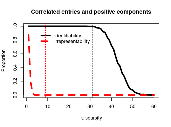
Figure 2: Graphs of functions $k\mapsto p^{X}_{\rm Idtf+}(k)$ and $k\mapsto p^{X}_{\rm IC+}(k)$ where $X$ is described in the setting above. The vertical lines represent the values $k=\frac{100}{2\log(300)}$ and $k=100\times\rho(100/300)$.

4 Numerical comparisons of sign estimators

Theorem 1 states that the sign estimators provided by thresholded LASSO or thresholded BPDN can recover ${\rm S}(\beta)$ as long as the identifiability condition is satisfied. Another way to recover ${\rm S}(\beta)$ is to use a sign estimator provided by the adaptive LASSO proposed in [40]. Indeed, as claimed in [40] or [20], if the weights for adaptive LASSO are based on an accurate estimator for $\beta$ one obtains a sign estimator that is consistent for ${\rm S}(\beta)$ under much weaker assumptions than the irrepresentability condition. In this section, we numerically compare the sign estimators obtained by LASSO, thresholded LASSO, thresholded BP and adaptive LASSO. We also include a comparison with LASSO-zero [9], which is a modification of the thresholded BP aimed at controlling the number of false discoveries.

4.1 Selection of the tuning parameter

As explained in [38, 36], a value of the optimal tuning parameter for sign recovery by thresholded LASSO is much smaller than the optimal value of the tuning parameter for LASSO sign estimator. Specifically:

• For the LASSO sign estimator, the tuning parameter must be large enough to prevent the inclusion of false detections.

• For the thresholded LASSO sign estimator, the tuning parameter should be chosen to achieve good separation between zero and non-zero elements of $\beta$. This requires good estimation rather than good selection properties. Here, the tuning parameter does not need to be large, as the threshold allows false detections to be eliminated.

4.1.1 The tuning parameter for the LASSO sign estimator

If $S(\beta)$ satisfies the irrepresentability condition, then Proposition 3 in the Appendix implies that one can choose a tuning parameter $\lambda_{L}$ such that, for sufficiently large $\beta$, $\mathbb{P}(S\left(\beta(\lambda_{L})\right)=S(\beta))$ is arbitrarily close to a given value from $(0,1)$ (e.g. $0.95$). According to the irrepresentability curve in Figure 1, the irrepresentability condition is satisfied with probability close to 1 if the elements of $X$ are iid $\mathcal{N}(0,1)$ random variables and $\beta$ contains $k=5$ non-zero elements. Therefore, in this setting, we choose $\lambda_{L}$ such that the probability of sign recovery converges to 0.95 and the probability of at least one false discovery (Family Wise Error Rate, FWER) converges to 0.05 when the signal magnitude tends to infinity. Since the irrepresentability condition is not satisfied for the remaining scenarios in our simulation study and thus the FWER cannot be controlled at a low level, the performances of LASSO are not reported.

4.1.2 The tuning parameter for the thresholded LASSO sign estimator

The tuning parameter can be chosen using the asymptotic theory of the Approximate Message Passing (AMP) algorithm for LASSO provided, for example, in [2, 28, 38]. In this theory, the elements of the design matrix are iid Gaussian $\mathcal{N}(0,1)$ variables and the components of $\beta$ are iid random variables from the mixture distribution $\Pi=(1-\gamma)\delta_{0}+\gamma\Pi^{\star}$, where $\delta_{0}$ is a point mass distribution concentrated at 0 and $\Pi^{\star}$ is an arbitrary fixed distribution. The asymptotic mean squared error of LASSO is derived under the assumption that the number of observations $n$ and the number of explanatory variables $p$ tend to infinity and that $n/p$ tends to $\delta>0$. Then the tuning parameter $\lambda_{AMP}$ is chosen such that the asymptotic mean squared error is minimal (see, e.g., the prescription in [38, 36]). As discussed in [38, 36], such a tuning parameter for any fixed value of Type I error allows maximizing the asymptotic power of the LASSO. In our simulation study, we used this asymptotically optimal $\lambda_{AMP}(k,t)$ for the parameter values: $\delta=n/p=100/300$, $\gamma=k/p=k/300$ and $\Pi^{\star}=1/2\delta_{t}+1/2\delta_{-t}$, where $\delta_{t}$ is a point mass distribution at $t$. The values $\lambda_{AMP}(k,t)$ were then used for the simulations in the independent case. In the “correlated” case, these values proved to be sub-optimal, so in this case we additionally obtained results for tuning parameters equal to $0.5\lambda_{AMP}(k,t)$, which provide much better empirical performance.

4.2 Selection of the threshold

We define the thresholded LASSO estimator (or the thresholded BP estimator) to be

$$\forall i\in\{1,\dots,p\},\widehat{\beta}^{\tau}_{i}:=\widehat{\beta}_{i}{\bf 1}_{\left\{\left|\widehat{\beta}_{i}\right|>\tau\right\}}\;.$$ (4)

Given a threshold $\tau>0$, we now define FWER as

$${\rm FWER}(\tau):=\mathbb{P}\left(\exists i\notin{\rm supp}(\beta),\left|\widehat{\beta}^{\tau}_{i}\right|\neq 0\right).$$

By taking $\tau_{\alpha}$ as the $1-\alpha$ quantile of the distribution of $\max\left\{|\widehat{\beta}_{i}|,i\notin{\rm supp}(\beta)\right\}$ we would control FWER exactly at the $\alpha$ level. However, $\tau_{\alpha}$ cannot be readily determined since $\beta$ is not known.

To obtain a threshold greater than $\tau_{\alpha}$ (and thus control for FWER at the $\alpha$ level), it seems appealing to consider the distribution of the supremum norm of the LASSO estimator (or BP estimator) in the complete null model when $\beta={\bf 0}$ [18]. For the BP estimator, Descloux and Sardy [9] propose the threshold $\tau^{\rm fn}_{\alpha}$ defined as the $1-\alpha$ quantile of $\max\left\{\left|\widehat{\beta}_{1}^{\rm fn}\right|,\dots,\left|\widehat{\beta}_{p}^{\rm fn}\right|\right\}$ where $\widehat{\beta}^{\rm fn}$ is the following estimator

$$\widehat{\beta}^{\rm fn}:=\text{ \rm argmin }\|\beta\|_{1}\text{ \rm subject to }X\beta=\varepsilon,\text{ \rm where $\varepsilon\sim\mathcal{N}_{n}(0,\sigma^{2}I)$}.$$

Unfortunately, if the vector $\beta$ contains some non-zero elements, this intuitive method yields a threshold $\tau^{\rm fn}_{\alpha}$ smaller than $\tau_{\alpha}$ and thus ${\rm FWER}(\tau^{\rm fn}_{\alpha})>\alpha$ (see also Su et al. [28] for further explanation).

The recently developed knockoff methodology [1, 5] provides control of False Discovery Rate (FDR). This control is achieved by adding additional control variables to the design matrix. Originally designed to control the FDR, the control variables also allow us to approximate the distribution of estimators corresponding to the zero components of $\beta$. In this numerical study, we informally use the model-free knockoffs proposed in [5] to approximate a threshold that controls the FWER at a certain level. The approach developed below is suitable for the situation when $X$ is a random matrix whose distribution is invariant to the permutation of the columns. In this setting, we can generate the knockoff variables one by one instead of generating the full $n\times p$ knockoff matrix (see Weinstein et al. [37] for a similar approach). Since adding the controlled variables may change some relevant properties (e.g. the identifiability condition for $\beta$), we should ideally add only one knockoff variable at a time when computing LASSO estimates. However, this would lead to a heavy computational burden on the procedure for estimating the relevant threshold. Therefore, in our simulation study, we use model-free knockoffs [5, 37] to generate $30=p/10$ controlled variables. Then Lasso or BP is run on the matrix augmented with these additional columns and the maximum of the absolute values of the regression coefficients over 30 controlled variables is stored. This step is repeated $10$ times and the total maximum of $p=300$ absolute values of regression coefficients over controlled variables is calculated. The whole procedure is repeated many times (1000 in this case) and the 0.95-quantile of the obtained maxima is used as a threshold to identify zero components of $\beta$. To be consistent with the setup of the simulations used to derive the irrepresentability and identifiability curves, we used the same two fixed design matrices $X$ as in Figure 1, while the positions of the $k$ sparse signals and the error terms were randomly generated for each of the 1000 replicates.

4.2.1 LASSO and Adaptive LASSO

In our numerical experiments, we chose the following values of tuning parameters for LASSO and adaptive LASSO:

• For LASSO, we chose $\lambda_{L}=81.18$ to control for FWER at the 0.05 level when $k=5$ and the covariates are independent.

• For adaptive LASSO, the weights are derived using initial estimates $\widehat{\beta}^{L}(\lambda_{AMP})$, where the tuning parameter is chosen according to the AMP theory, described above. For $i\in\{1,\dots,p\}$, the weights $w_{i}$ are defined as $w_{i}:=1/(|\widehat{\beta_{i}}^{L}(\lambda_{AMP})|+10^{-7})$. With these weights and the tuning parameter $\lambda_{L}$ described above, the adaptive LASSO has the following expression

  $$\widehat{\beta}^{\rm adapt}:=\underset{\beta\in\mathbb{R}^{p}}{\text{\rm argmin }}\frac{1}{2}\|Y-X\beta\|_{2}^{2}+\lambda_{L}\sum_{i=1}^{p}w_{i}|\beta_{i}|.$$ (5)

In all our simulations, LASSO is computed using glmnet R package.

4.2.2 LASSO-zero from [9]

Given iid $n\times q$ standard Gaussian matrices $G^{(1)},\dots,G^{(M)}$, we consider the following basis pursuit minimizers:

$$\forall k\in\{1,\dots,M\},(\hat{\beta}^{(k)},\hat{\gamma}^{(k)}):=\underset{b\in\mathbb{R}^{p},c\in\mathbb{R}^{q}}{\text{\rm argmin }}\|b\|_{1}+\|c\|_{1}\text{ \rm subject to }y=Xb+G^{(k)}c.$$

Now, given a threshold $\tau>0$, we can define the LASSO-zero estimator $\hat{\beta}^{{\rm lass0}(q,M)}_{\tau}$ as follows:

$$\forall i\in\{1,\dots,p\},\hat{\beta}^{med}_{i}={\rm median}\{\hat{\beta}^{(1)}_{i},\dots,\hat{\beta}^{(M)}_{i}\}\text{ \rm and }\hat{\beta}_{\tau,i}^{{\rm lass0}(q,M)}=\hat{\beta}^{med}_{i}{\bf 1}(|\hat{\beta}^{med}_{i}|>\tau).$$

One can use the knowledge that $\sigma=1$, to compute the QUT threshold $\tau$ as the $1-\alpha$ quantile of $\|\hat{\beta}^{med}\|_{\infty}$ when $\beta={\bf 0}$. Otherwise, one can also pivotize the $\|\hat{\beta}^{med}\|_{\infty}$ statistic to compute this threshold (see [9] for details).

4.3 Numerical comparisons

All numerical experiments are performed with the two $100\times 300$ design matrices $X$ already used in Figure 1 and in Section 3.1. We set $\beta\in\mathbb{R}^{p}$ such that $k:={\rm card}({\rm supp}(\beta))$ with $k\in\{5,20\}$ and the $k$ elements of ${\rm supp}(\beta)$ are drawn without replacement from $\{1,\dots,p\}$. The non-zero components of $\beta$ are sampled from the distribution $P(\beta_{i}=t)=P(\beta_{i}=-t)=0.5$ with $t>0$. Additionally, when the columns of $X$ are correlated, we consider the constellation in which all non-zero coefficients are equal to $t$. In all simulations, the error term is generated as $\varepsilon\sim\mathcal{N}(0,Id_{n})$.

Figures 3-4 show the comparison between the following sign estimators.

• The sign estimator L from LASSO with $\lambda=\lambda_{L}$.

• The sign estimator aL from the adaptive LASSO, described in (5).

• The sign estimator BPk from the thresholded BP, where the threshold is given by the ”knockoff” method described above.

• The sign estimator Lk from the thresholded LASSO with $\lambda=\lambda_{AMP}$ and with a threshold given by the “knockoff” method described above.

• The sign estimator Lks from the thresholded LASSO with $\lambda=0.5\lambda_{AMP}$ and with a threshold given by the ”knockoff” method described above.

• The sign estimator Lz of LASSO-zero, where $M=30,q=n$. The QUT threshold is not data driven and is computed as the $0.95$ quantile of $\|\hat{\beta}^{med}\|_{\infty}$ when $\beta={\bf 0}$.

• The sign estimator Lzp of LASSO-zero when $M=30,q=n$. The QUT threshold is data-driven and is computed by pivotizing the statistic $\|\hat{\beta}^{med}\|_{\infty}$, as explained in [9].

We give the curves representing the following statistical properties as a function of $t>0$:

• Probability is the proportion of 1000 replicates for which the sign is recovered.

• FWER is the proportion of 1000 replicates for which at least one zero component of $\beta$ is not estimated to be zero.

FWER is directly related to the probability of sign recovery, namely $FWER\geq\alpha$ implies that the probability of sign recovery is less than $1-\alpha$. The sign estimators L, BPk, Lk and Lks were specifically designed to control for FWER at the 0.05 level.

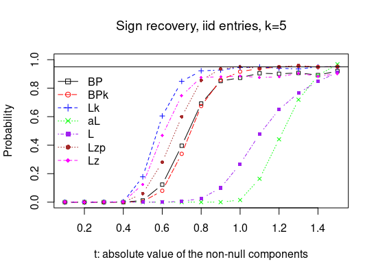
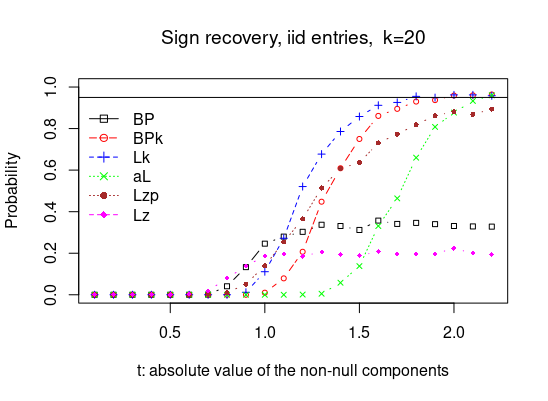
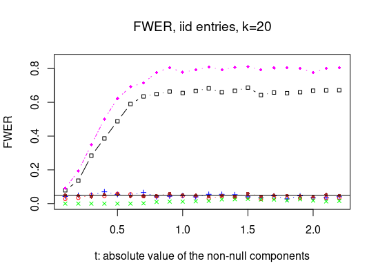
Figure 3: This figure shows the FWER and the probability of recovering $S(\beta)$ for each sign estimator and when $X$ contains iid $\mathcal{N}(0,1)$ entries. The graphs on the left show the probability of recovering $S(\beta)$ (on the y-axis) as a function of $t$ (on the x-axis), where $t$ indicates how large the non-zero components of $\beta$ are. The graphs on the right show the FWER (on the y-axis) as a function of $t$ (on the x-axis).

If $k=5$ and the elements of $X$ are iid normal variables, then the irrepresentability condition holds and LASSO can recover the true model. Figure 3 shows that in this case the upper bound on the probability of recovering the sign given in Proposition 3 is achieved by LASSO and the FWER is controlled. However, for moderately large signals, the probability of recovering $S(\beta)$ by LASSO is much smaller than by the thresholded versions of BP and Lasso, as well as by Lasso-zero. If $k=20$, the irrepresentability condition is not satisfied, but the identifiability condition holds, thus the thresholded LASSO and the thresholded BP identify the sign of $\beta$ when non-zero elements are large and the threshold is properly calibrated.

Figure 3 shows that thresholds for BP or Lz, which are not data-driven and are computed in the complete null model (i.e. when $\beta={\bf 0}$) do not control the FWER when $\beta$ has many large components (intuitively, when $\beta$ is far from ${\bf 0}$). Consequently, BP or Lz cannot recover $S(\beta)$ with a large probability. Instead, our heuristic application of the knockoff method, as well as LASSO-zero when the threshold is data-driven, allow us to almost perfectly control FWER at $0.05$. Consequently, when the non-zero components of $\beta$ are large enough, the sign estimators derived from Lk, BPk, and Lzp recover $S(\beta)$ with probability close to $0.95$. Among these methods, the thresholded LASSO estimator Lk with $\lambda$ selected by AMP theory systematically has the highest probability of recovering $S(\beta)$ for moderately large signals.

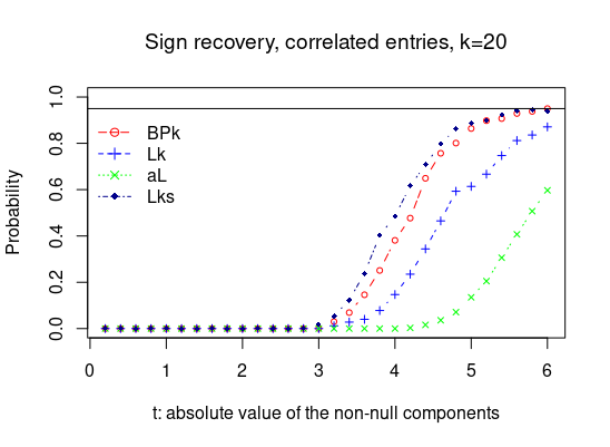
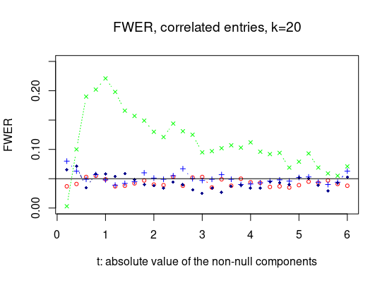
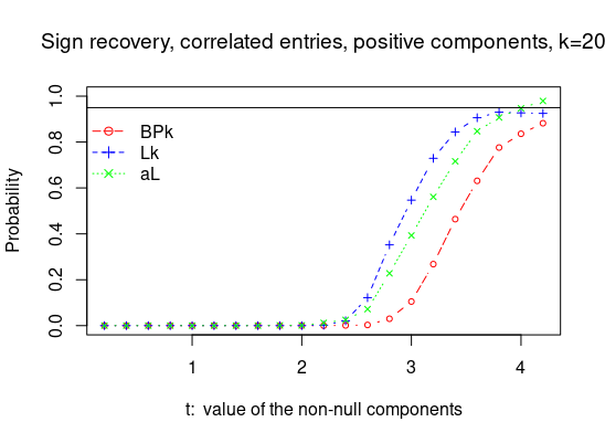
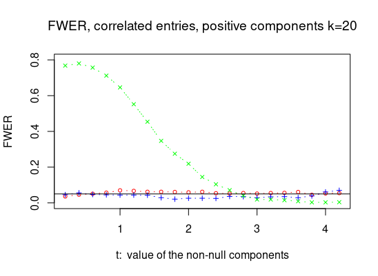
Figure 4: This figure shows the FWER and the probability of recovering $S(\beta)$ for each sign estimator when $X$ has strongly correlated columns. The plots on the left show the probability of recovery of $S(\beta)$ (on the y-axis) as a function of $t$ (on the x-axis), where $t$ measures how large the non-zero components of $\beta$ are. The graphs on the right show the FWER (on the y-axis) as a function of $t$.

Figure 4 shows the results of the simulation study for the design matrix $X$ with very highly correlated columns. In this setting, the probability of recovering $S(\beta)$ by LASSO-zero was very close to zero, and for clarity of presentation, LASSO-zero is not included in Figure 4.

Figure 4 confirms the numerical experiments given in Figure 3. In particular, thresholded BP and thresholded LASSO can recover $S(\beta)$ when the threshold is well calibrated and the non-zero components of $\beta$ are large enough. If the tuning parameter is chosen correctly, thresholded LASSO recovers $S(\beta)$ with a higher probability than thresholded BP. Similar to the case of independent entries, our heuristic knockoff approach allows to control FWER at the 0.05 level.

4.4 Numerical experiments with the design matrix from the riboflavin dataset

In this section, we consider the same simulation setting as in [9], which deals with the riboflavin dataset [3]. The design matrix $X$ contains expression levels of $p=4088$ genes for $n=71$ Bacillus subtilis bacteria. The matrix is mean-centered (for each $j\in\{1,\dots,p\},\sum_{i=1}^{n}X_{ij}=0$) and standardized (for each $j\in\{1,\dots,p\},\frac{1}{n-1}\sum_{i=1}^{n}X_{ij}^{2}=1$). Figure 5 shows irrepresentability and identifiability curves of this design matrix.

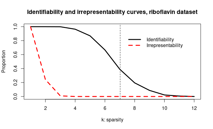
Figure 5: Graphs of the functions $k\mapsto p^{X}_{\rm Idtf}(k)$ and $k\mapsto p^{X}_{\rm IC}(k)$ where $k\in\{1,\dots,12\}$ and $X$ is the matrix from the riboflavin dataset. The equation of the vertical line is $k=n\rho(n/p)$.

The identifiability and irrepresentability curves shown in Figure 5 confirm the numerical experiments reported in Descloux and Sardy [9]. In particular, the probability of sign recovery by LASSO reported in panel (c) of Figure 6 in [9] is below the irrepresentability curve from Figure 5 and the probability of sign recovery by LASSO-zero is below the identifiability curve.

We also ran the simulations comparing LASSO-zero and thresholded LASSO on the riboflavin dataset. In this study, we set $k:={\rm card}({\rm supp}(\beta))\in\{1,2,3\}$ (so that the identifiability condition holds), and the non-zero coefficients are set to 2 with random signs. In addition to the probability of sign recovery and the FWER, we also estimate the False Discovery Rate (FDR) and the True Positive Rate (TPR).

• FDR is the mean of 1000 replicates of the False Discovery Proportion (FDP), where the FDP is defined as follows:

  $$FDP=\frac{{\rm card}(\{i\notin{\rm supp}(\beta)|\hat{\beta}_{i}\neq 0\})}{\max\{{\rm card}({\rm supp}(\hat{\beta})),1\}}.$$

• TPR is the mean of 1000 replicates of the True Positive Proportion (TPP), where the TPP is defined as follows:

  $$TPP=\frac{{\rm card}({\rm supp}(\beta)\cap{\rm supp}(\hat{\beta}))}{{\rm card}({\rm supp}(\beta))}.$$

For the thresholded LASSO, we selected the tuning parameter by cross-validation. To estimate the threshold, we used the heuristic knockoff procedure described above, where for each run of LASSO we added $q=p/8=511$ columns to the design matrix $X$, drawn from the multivariate normal distribution $N(0,\Gamma)$, where $\Gamma_{ii}=1$ and $\Gamma_{ij}=\frac{1}{p(p-1)(n-1)}\sum_{i\neq j}X_{i}^{\prime}X_{j}=0.0292$.

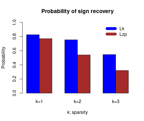
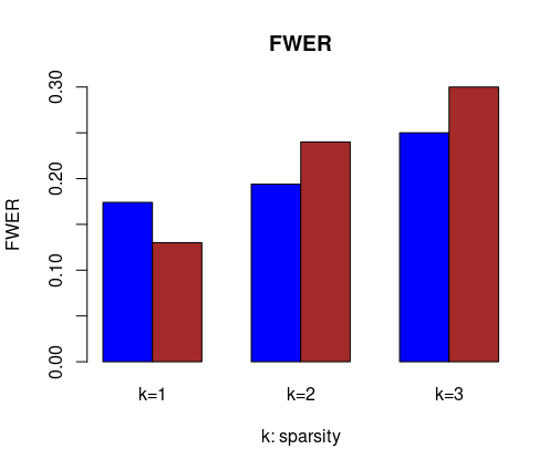
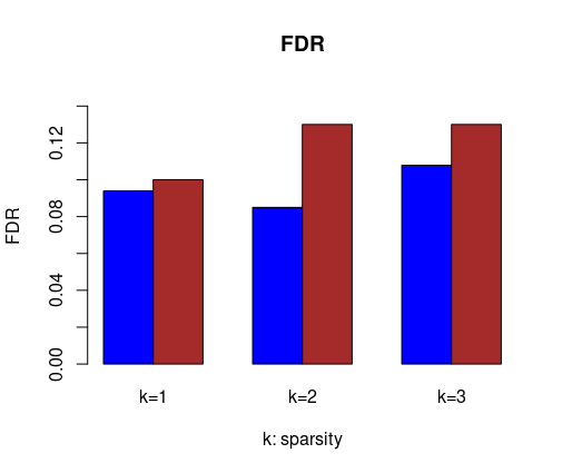
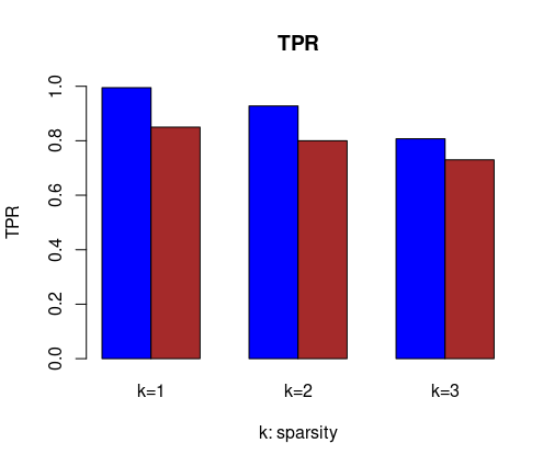
Figure 6: This figure provides the probability of sign recovery, FWER, FDR and TPR of LASSO-zero (Lzp) and thresholded LASSO (Lk) as a function of the sparsity $k\in\{1,2,3\}$.

Figure 6 shows that LASSO-zero and thresholded LASSO have FWER above the assumed value of 0.05. This is not surprising since the gene expressions are not exactly normally distributed. However, the FWER of both methods is still quite low (below 0.3) and the FDR is kept close to 0.1. Since the correlations between columns in the design matrix are not too large, the thresholded LASSO and LASSO-zero show similar performance. However, the probability of sign recovery and TPR is systematically larger for thresholded LASSO, which also has smaller FWER and FDR.

5 Conclusion

The focus of this article is on the theoretical properties of sign estimators derived from LASSO, thresholded LASSO, and thresholded BPDN . When $S(\beta)$ is identifiable with respect to the $\ell_{1}$ norm and when non-zero components of $\beta$ tends to infinity, we have shown that sign estimators derived from thresholded LASSO and thresholded BPDN recover $S(\beta)$. On the other hand, if $S(\beta)$ is not identifiable with respect to the $\ell_{1}$ norm, sign estimators derived from thresholded LASSO and thresholded BPDN cannot recover $S(\beta)$.

We introduced irrepresentability and identifiability curves that provide information about the probability of sign recovery by LASSO or thresholded LASSO and thresholded BPDN as a function of the number of non-zero elements in the vector of regression coefficients.

The performances of the sign estimators derived from LASSO, thresholded LASSO and thresholded BPDN obviously depend on the tuning parameters and the threshold. We have illustrated that AMP theory and the knockoff method are useful to select these parameters. Our simulations show that thresholded LASSO and thresholded BPDN sign estimators outperform the adaptive LASSO and LASSO sign estimators.

6 Appendix

6.1 Sign recovery with LASSO sign estimator

The upper bound for sign recovery given in Proposition 3 appears in Lemma 3 of Wainwright [35] as a technical result establishing the irrepresentability condition (Theorem 2 in Wainwright [35]). According to Proposition 3, if $\beta$ is identifiable with respect to the $\ell_{1}$-norm, this upper bound is asymptotically reached as soon as $\min\{|\beta_{i}|,i\in{\rm supp}(\beta)\}$ tends to $+\infty$.

Lemma 1 (Lemma 3 from [35] )

Let $I:={\rm supp}(\beta)$ and let $X_{I},X_{\overline{I}}$ be matrices whose columns are $(X_{i})_{i\in I}$ and $(X_{i})_{i\notin I}$, respectively. Let us assume that $\ker(X_{I})=\{{\bf 0}\}$ and let $\zeta_{X,\lambda,S(\beta)}:=X_{\overline{I}}^{\prime}X_{I}(X_{I}^{\prime}X_{I})^{-1}S(\beta_{I})+\frac{1}{\lambda}X_{\overline{I}}^{\prime}\left(Id-X_{I}(X_{I}^{\prime}X_{I})^{-1}X_{I}^{\prime}\right)\varepsilon.$

The following upper bound for the sign recovery holds.

$$\mathbb{P}\left(S(\widehat{\beta}^{\rm L}(\lambda))=S(\beta)\right)\leq\mathbb{P}\left(\left\|\zeta_{X,\lambda,S(\beta)}\right\|_{\infty}\leq 1\right).$$

Proposition 3

Assume that the assumptions of Lemma 1 hold. Moreover, assume that the sequence $(\beta^{(r)})$ in $\mathbb{R}^{p}$ satisfies Assumption 1. If $s^{0}$ is identifiable with respect to the $\ell_{1}$-norm, then the following asymptotic results hold.

Sharpness of the upper bound:

Asymptotically, the upper bound is obtained.

$$\limsup_{r\to+\infty}\mathbb{P}\left(S(\widehat{\beta}^{\rm L}(\lambda,r))=s^{0}\right)\leq\mathbb{P}\left(\left\|\zeta_{X,\lambda,s^{0}}\right\|_{\infty}\leq 1\right),$$

$$\liminf_{r\to+\infty}\mathbb{P}\left(S(\widehat{\beta}^{\rm L}(\lambda,r))=s^{0}\right)\geq\mathbb{P}\left(\left\|\zeta_{X,\lambda,s^{0}}\right\|_{\infty}<1\right).$$

Asymptotic control of FWER:

Let us define $\mathbb{P}\left(\left\|\zeta_{X,\lambda,s^{0}}\right\|_{\infty}<1\right)=\gamma$ and $\mathbb{P}\left(\left\|\zeta_{X,\lambda,s^{0}}\right\|_{\infty}\leq 1\right)=\bar{\gamma}$. The sign of the non-zero elements of $\beta^{(r)}$ is correctly identified with probability converging to $1$ and the FWER is controlled at the $1-\gamma$ level.

$$\lim_{r\to+\infty}\mathbb{P}\left(\forall i\in I,S(\widehat{\beta}_{i}^{\rm L}(\lambda,r))=s^{0}_{i}\right)=1,$$

$$\limsup_{r\to+\infty}\mathbb{P}\left(\exists i\notin I,\widehat{\beta}_{i}^{\rm L}(\lambda,r)\neq 0\right)\leq 1-\gamma,$$

$$\liminf_{r\to+\infty}\mathbb{P}\left(\exists i\notin I,\widehat{\beta}_{i}^{\rm L}(\lambda,r)\neq 0\right)\geq 1-\bar{\gamma}.$$

Remark 1

The results in Proposition 3 are quite straightforward when $X$ is orthogonal (i.e. when $X^{\prime}X=I$). Indeed, in this case the upper bound is simply the probability that zero components of $\beta$ are simultaneously estimated to $0$, namely $\mathbb{P}(\forall i\notin{\rm supp}(\beta),\hat{\beta}^{\rm L}_{i}(\lambda)=0)$

If $\varepsilon$ has a covariance matrix $\sigma^{2}Id_{n}$, one can obtain asymptotic results by fixing $\beta$ and letting $\sigma$ tend to $0$. However, unlike in our asymptotic setting described in Assumption 1, such asymptotic results are very poor and give no information about the FWER. Indeed, when $\sigma$ tends to $0$, the upper bound tends to $0$ or $1$, depending on whether the irrepresentable condition for $\beta$ holds or not.

Let us remind that the FWER is equal to $\mathbb{P}(\exists i\notin{\rm supp}(\beta),\widehat{\beta}^{L}_{i}\neq 0)$. According to Proposition 3, when non-null components of $\beta$ are infinitely large, the FWER is controlled at level $1-\mathbb{P}\left(\left\|\zeta_{X,\lambda,{\rm sign}(\beta)}\right\|_{\infty}<1\right)$. To our knowledge, it is first theoretical result providing a formula for the FWER. Hereafter, let us provide some comments about the FWER control.

• To provide a specific value for $\lambda$ allowing to control the FWER one needs to know the distribution of $\varepsilon$. For example, when the distribution of $\varepsilon$ is known and $\beta={\bf 0}$ one controls the FWER at level $\alpha$ by taking $\lambda$ as the $1-\alpha$ quantile of $\|X^{\prime}\varepsilon\|_{\infty}$. Let us point out that when $\varepsilon_{1},\dots,\varepsilon_{p}$ are iid and the variance $\sigma^{2}$ of these components is unknown then $\sigma^{2}$ can be consistently estimate as explained in [10].

• It is easier to control the FWER when $X$ is a random matrix whose distribution is symmetric and invariant by columns permutation than when $X$ is a fixed design matrix. Indeed, when $X$ is random, the distribution of $\zeta_{X,\lambda,S(\beta)}$ just depends from the sparsity of $\beta$ and not on $S(\beta)$.

• Let $k\in\{1,\dots,p\}$ and let $U_{k}$ be the set $\{u\in\{-1,0,1\}^{p}\mid{\rm card}({\rm supp}(u))=k\}$ and let us assume that $\beta\in U_{k}$. When $X$ is a random matrix whose distribution is symmetric and invariant by columns permutation by taking $\lambda_{\alpha}$ such that $\mathbb{P}(\|\zeta_{X,\lambda_{\alpha},u_{0}}\|<1)=1-\alpha$ one controls asymptotically the FWER at level $\alpha$ (where $u_{0}:=(1,\dots,1,0,\dots,0)\in U_{k}$). Such a tuning parameter $\lambda_{\alpha}$ is easy to infer by Monte Carlo simulations. When $X$ is fixed, by taking $\lambda_{\alpha}$ as follows

  $$\frac{1}{{\rm card}(U_{k})}\sum_{u\in U_{k}}\mathbb{P}(\|\zeta_{X,\lambda_{\alpha},u}\|<1)=1-\alpha,$$ (6)

  then the average value of the FWER with respect to $\beta\in U_{k}$ is $1-\alpha$ (where non-null components of $\beta$ are infinitely large). Again $\lambda_{\alpha}$ is easy to infer. In the numerical experiment, the tuning parameter was selected by solving equation (6).

6.2 Proof of the Proposition 3

First, let us provide lemmas which are useful to prove both Proposition 3 and Theorem 1. Lemma 3 partially proves Proposition 3. Indeed, according to this Lemma, when $(\beta^{(r)})_{r\in\mathbb{N}}$ is a sequence of $\mathbb{R}^{p}$ satisfying assumptions 1 then the following asymptotic result holds

$$\lim_{r\to+\infty}\mathbb{P}\left(\forall i\in{\rm supp}(s^{0}),S(\widehat{\beta}^{\rm L}_{i}(\lambda,r))=s^{0}_{i}\right)=1.$$

Lemma 2

Let $(\beta^{(r)})_{r\in\mathbb{N}}$ be a sequence of $\mathbb{R}^{p}$ satisfying the conditions 1) and 2) of Assumption 1, let us assume that $s^{0}$ is identifiable with respect to the $\ell_{1}$ norm and let us set $u_{r}=\|\beta^{(r)}\|_{1}$ then

$$\lim_{r\to+\infty}\frac{\widehat{\beta}^{\rm L}(\varepsilon,r)-\beta^{(r)}}{u_{r}}=0.$$

Proof: Because $\widehat{\beta}^{\rm L}(\varepsilon,r)$ is the LASSO estimator as defined in (2) then the following inequality occurs

$$\frac{1}{2}\|Y-X\widehat{\beta}^{\rm L}(\varepsilon,r)\|^{2}_{2}+\lambda\|\widehat{\beta}^{\rm L}(\varepsilon,r)\|_{1}\leq\frac{1}{2}\|Y-X\beta^{(r)}\|^{2}_{2}+\lambda\|\beta^{(r)}\|_{1}.$$

Since $Y-X\beta^{(r)}=\varepsilon$ one may deduce the following inequalities

$$\lambda\|\widehat{\beta}^{\rm L}(\varepsilon,r)\|_{1}\leq\frac{1}{2}\|\varepsilon\|^{2}_{2}+\lambda\|\beta^{(r)}\|_{1},$$

$$\Rightarrow \|\widehat{\beta}^{\rm L}(\varepsilon,r)/u_{r}\|_{1}\leq\frac{\|\varepsilon\|^{2}_{2}}{2\lambda u_{r}}+1.$$ (7)

In addition, Cauchy-Schwarz inequality gives the following implications

$$\frac{1}{2}\|\varepsilon+X\beta^{(r)}-X\widehat{\beta}^{\rm L}(\varepsilon,r)\|^{2}_{2}+\lambda\|\widehat{\beta}^{\rm L}(\varepsilon,r)\|_{1}\leq\frac{1}{2}\|\varepsilon\|^{2}_{2}+\lambda\|\beta^{(r)}\|_{1},$$

$$\Rightarrow -\|\varepsilon\|_{2}\|X\beta^{(r)}-X\widehat{\beta}^{\rm L}(\varepsilon,r)\|_{2}+\frac{1}{2}\|X\beta^{(r)}-X\widehat{\beta}^{\rm L}(\varepsilon,r)\|^{2}_{2}+\lambda\|\widehat{\beta}^{\rm L}(\varepsilon,r)\|_{1}\leq\lambda\|\beta^{(r)}\|_{1},$$

$$\Rightarrow -\frac{\|\varepsilon\|_{2}}{u_{r}}\left\|X\left(\frac{\widehat{\beta}^{\rm L}(\varepsilon,r)-\beta^{(r)}}{u_{r}}\right)\right\|_{2}+\frac{1}{2}\left\|X\left(\frac{\widehat{\beta}^{\rm L}(\varepsilon,r)-\beta^{(r)}}{u_{r}}\right)\right\|^{2}_{2}+\frac{\lambda}{u_{r}}\left\|\frac{\widehat{\beta}^{\rm L}(\varepsilon,r)}{u_{r}}\right\|_{1}\leq\frac{\lambda}{u_{r}}.$$ (8)

Because $u_{r}$ tends to $+\infty$ then, according to (7), the sequence $((\widehat{\beta}^{\rm L}(\varepsilon,r)-\beta^{(r)})/u_{r})_{r\in\mathbb{N}^{*}}$ is bounded since the following superior limit is finite

$$\limsup_{r\to+\infty}\left\|\frac{\widehat{\beta}^{\rm L}(\varepsilon,r)-\beta^{(r)}}{u_{r}}\right\|_{1}\leq 2.$$

Consequently, to prove that $\lim_{r\to+\infty}(\widehat{\beta}^{\rm L}(\varepsilon,r)-\beta^{(r)})/u_{r}={\bf 0}$ it is sufficient to show that ${\bf 0}$ is the unique limit point of this sequence. Let $((\widehat{\beta}^{\rm L}(\varepsilon,\phi(r))-\beta^{(\phi(r))})/u_{\phi(r)})_{r\in\mathbb{N}^{*}}$ be a converging subsequence to $l$ (with $\phi:\mathbb{N}^{*}\to\mathbb{N}^{*}$ strictly increasing) and without loss of generality, let us assume $\lim_{r\to+\infty}\widehat{\beta}^{\rm L}(\varepsilon,\phi(r))/u_{\phi(r)}=v$ and $\lim_{r\to+\infty}\beta^{(\phi(r))}/u_{\phi(r)}=v^{\prime}$ so that $l=v-v^{\prime}$. By (7) and (8) one may deduce that

$$Xv=Xv^{\prime}\text{ \rm and }\|v\|_{1}\leq 1.$$

Since, whatever $r\geq 0$, we have $S(\beta^{(\phi(r))}/u_{\phi(r)})=s^{0}$ where $s^{0}$ is identifiable with respect to the $\ell_{1}$ norm then, according to Proposition 2, one may deduce that $\beta^{(\phi(r))}/u_{\phi(r)}$ is an unitary vector satisfying the identifiability condition. Consequently, $\|v^{\prime}\|_{1}=1$ and $v^{\prime}$ is identifiable with respect to the $\ell_{1}$ norm. Consequently, $v=v^{\prime}$ and thus $l={\bf 0}$ is the unique limit point, which implies that

$$\lim_{r\to+\infty}\frac{\widehat{\beta}^{\rm L}(\varepsilon,r)-\beta^{(r)}}{u_{r}}={\bf 0}.$$

$\hfill\square$

For the proof of Lemma 2, we have not used the third condition of Assumption 1. This condition, under which the smallest non-null component of $\beta^{(r)}$ is not asymptotically infinitely smaller than $\|\beta^{(r)}\|_{\infty}$, is useful to prove Lemma 3.

Lemma 3

Let $(\beta^{(r)})_{r\in\mathbb{N}}$ be a sequence of $\mathbb{R}^{p}$ satisfying Assumption 1, then

$$\lim_{r\to+\infty}\mathbb{P}(\forall i\in{\rm supp}(s^{0}),S(\widehat{\beta}^{\rm L}_{i}(\lambda,r))=s^{0}_{i})=1.$$

Proof: Let $\varepsilon$ be a fixed vector in $\mathbb{R}^{p}$. According to the third condition of Assumption 1 we have $\min\{|\beta^{(r)}_{i}|,i\in{\rm supp}(s^{0})\}/\|\beta^{(r)}\|_{\infty}\geq q>0$, consequently the following inequalities occur

$$\forall i\in{\rm supp}(s^{0}),s^{0}_{i}\frac{\widehat{\beta}_{i}^{\rm L}(\varepsilon,\lambda,r)-\beta_{i}^{(r)}}{\|\beta^{(r)}\|_{\infty}}=\frac{s^{0}_{i}\widehat{\beta}_{i}^{\rm L}(\varepsilon,\lambda,r)}{\|\beta^{(r)}\|_{\infty}}-\frac{|\beta_{i}^{(r)}|}{\|\beta^{(r)}\|_{\infty}}\leq\frac{s^{0}_{i}\widehat{\beta}_{i}^{\rm L}(\varepsilon,\lambda,r)}{\|\beta^{(r)}\|_{\infty}}-q.$$

According to Lemma 2, the following inequality occurs

$$0=\liminf_{r\to+\infty}s^{0}_{i}\frac{\widehat{\beta}_{i}^{\rm L}(\varepsilon,\lambda,r)-\beta_{i}^{(r)}}{\|\beta^{(r)}\|_{\infty}}\leq\liminf_{r\to+\infty}\frac{s^{0}_{i}\widehat{\beta}_{i}^{\rm L}(\varepsilon,\lambda,r)}{\|\beta^{(r)}\|_{\infty}}-q.$$

Which implies that for $r$ large enough $s^{0}_{i}\widehat{\beta}_{i}^{\rm L}(\varepsilon,\lambda,r)>0$ and thus $S(\widehat{\beta}_{i}^{\rm L}(\varepsilon,\lambda,r))=s^{0}_{i}$. When $\varepsilon$ is no longer fixed then, for $i\in{\rm supp}(s^{0})$, almost surely $S(\widehat{\beta}_{i}^{\rm L}(r))$ converges to $s^{0}_{i}$ and consequently

$$\lim_{r\to+\infty}\mathbb{P}\left(\forall i\in{\rm supp}(s^{0}),S(\widehat{\beta}^{\rm L}_{i}(\lambda,r))=s^{0}_{i}\right)=1.$$

$\hfill\square$

Proof of Proposition 3:
Let us remind that the vector $\widehat{\beta}^{\rm L}(\lambda)$ is the LASSO estimator if and only if the following two inequalities occur simultaneously.

$$X_{A}^{\prime}(Y-X\widehat{\beta}^{\rm L}(\lambda)) = \lambda S(\widehat{\beta}^{\rm L}_{A}(\lambda)),\text{ \rm where }A={\rm supp}(\widehat{\beta}^{\rm L}(\lambda)),$$ (9)

$$\|X_{\overline{A}}^{\prime}(Y-X\widehat{\beta}^{\rm L}(\lambda))\|_{\infty} \leq \lambda.$$ (10)

Sharpness of the upper bound) Since the upper bound depends only on $s^{0}$ and not on how large the non-null components $\beta^{(r)}$ are then

$$\limsup_{r\to+\infty}\mathbb{P}\left(S(\widehat{\beta}^{\rm L}(\lambda,r))=s^{0}\right)\leq\mathbb{P}\left(\left\|\zeta_{X,\lambda,s^{0}}\right\|_{\infty}\leq 1\right).$$

Finally, it must be proven that $\liminf_{r\to+\infty}\mathbb{P}\left(S(\widehat{\beta}^{\rm L}(\lambda,r))=s^{0}\right)\geq\mathbb{P}\left(\left\|\zeta_{X,\lambda,s^{0}}\right\|_{\infty}<1\right)$. Let us remind that $I={\rm supp}(s^{0})$ and let us assume that the following events hold simultaneously

$$X_{I}^{\prime}(Y-X\widehat{\beta}^{\rm L}(\lambda))=\lambda s^{0}_{I}\text{ \rm and }\underbrace{\left\|X_{\overline{I}}^{\prime}X_{I}(X_{I}^{\prime}X_{I})^{-1}\lambda s^{0}_{I}+X_{\overline{I}}^{\prime}\left(Id-X_{I}(X_{I}^{\prime}X_{I})^{-1}X_{I}^{\prime}\right)\varepsilon\right\|_{\infty}<\lambda}_{=\left\|\zeta_{X,\lambda,s^{0}}\right\|_{\infty}<1}.$$ (11)

We aim to show that the inequalities given above imply that $\widehat{\beta}^{\rm L}_{\overline{I}}(\lambda)={\bf 0}$. For convenience, let us set $H$ be the projection matrix $H:=X_{I}(X_{I}^{\prime}X_{I})^{-1}X_{I}^{\prime}$. When (11) occurs then the following inequalities holds

$$\left\|X_{\overline{I}}^{\prime}H(Y-X\widehat{\beta}^{\rm L}(\lambda))+X_{\overline{I}}^{\prime}\left(Id-H\right)\varepsilon\right\|_{\infty} < \lambda,$$

$$\left\|X_{\overline{I}}^{\prime}\left(H(Y-X\widehat{\beta}^{\rm L}(\lambda))+(Id-H)\varepsilon\right)\right\|_{\infty} < \lambda,$$

$$\left\|X_{\overline{I}}^{\prime}\left(Y-X\widehat{\beta}^{\rm L}(\lambda)+X_{\overline{I}}\widehat{\beta}^{\rm L}_{\overline{I}}(\lambda)-HX_{\overline{I}}\widehat{\beta}^{\rm L}_{\overline{I}}(\lambda)\right)\right\|_{\infty} < \lambda.$$ (12)

Inequality (12) comes from the following two identities

$$HY = H(X\beta^{(r)})+H\varepsilon=H(X_{I}\beta_{I}^{(r)})+H\varepsilon=X_{I}\beta_{I}^{(r)}+H\varepsilon=X(\beta^{(r)})+H\varepsilon\text{ \rm and},$$

$$HX\widehat{\beta}^{\rm L}(\lambda) = HX_{I}\widehat{\beta}^{\rm L}_{I}(\lambda)+HX_{\overline{I}}\widehat{\beta}^{\rm L}_{\overline{I}}(\lambda)=X_{I}\widehat{\beta}^{\rm L}_{I}(\lambda)+HX_{\overline{I}}\widehat{\beta}^{\rm L}_{\overline{I}}(\lambda)=X\widehat{\beta}^{\rm L}(\lambda)-X_{\overline{I}}\widehat{\beta}^{\rm L}_{\overline{I}}(\lambda)+HX_{\overline{I}}\widehat{\beta}^{\rm L}_{\overline{I}}(\lambda).$$

Let $v$ be the vector $v:=X_{\overline{I}}^{\prime}\left(Y-X\widehat{\beta}^{\rm L}(\lambda)+X_{\overline{I}}\widehat{\beta}^{\rm L}_{\overline{I}}(\lambda)-HX_{\overline{I}}\widehat{\beta}^{\rm L}_{\overline{I}}(\lambda)\right)$. We are going to see that inequality (12) implies that $\widehat{\beta}^{\rm L}_{\overline{I}}(\lambda)={\bf 0}$. Let us assume that $\widehat{\beta}^{\rm L}_{\overline{I}}(\lambda)\neq{\bf 0}$ then, on the one hand, the following inequality occurs

$$\widehat{\beta}^{\rm L}_{\overline{I}}(\lambda)^{\prime}v\leq\|\widehat{\beta}^{\rm L}_{\overline{I}}(\lambda)\|_{1}\|v\|_{\infty}<\lambda\|\widehat{\beta}^{\rm L}_{\overline{I}}(\lambda)\|_{1}.$$ (13)

According to (9) the identity $\widehat{\beta}^{\rm L}_{i}(\lambda)X_{i}^{\prime}(Y-X\widehat{\beta}^{\rm L}(\lambda))=\lambda|\widehat{\beta}^{\rm L}_{i}(\lambda)|$ occurs. Consequently, on the other hand, the following inequalities hold

$$\widehat{\beta}^{\rm L}_{\overline{I}}(\lambda)^{\prime}v = \widehat{\beta}^{\rm L}_{\overline{I}}(\lambda)^{\prime}X_{\overline{I}}^{\prime}\left(Y-X\widehat{\beta}^{\rm L}(\lambda)+X_{\overline{I}}\widehat{\beta}^{\rm L}_{\overline{I}}(\lambda)-HX_{\overline{I}}\widehat{\beta}^{\rm L}_{\overline{I}}(\lambda)\right),$$ (14)

$$= \lambda\|\widehat{\beta}^{\rm L}_{\overline{I}}(\lambda)\|_{1}+\widehat{\beta}^{\rm L}_{\overline{I}}(\lambda)^{\prime}X_{\overline{I}}^{\prime}(Id-H)X_{\overline{I}}\widehat{\beta}^{\rm L}_{\overline{I}}(\lambda),$$

$$\geq \lambda\|\widehat{\beta}^{L}_{\overline{I}}(\lambda)\|_{1}.$$

The last inequality occurs because the projection matrix $Id-H$ is positive semi-definite. Inequalities (13) and (14) provide a contradiction which implies that $\widehat{\beta}^{\rm L}_{\overline{I}}(\lambda)={\bf 0}$.
According to (9), the following implication holds

$$S(\widehat{\beta}^{\rm L}_{I}(\lambda,r))=s^{0}_{I}\Rightarrow X_{I}^{\prime}(Y-X\widehat{\beta}^{\rm L}(\lambda,r))=\lambda s^{0}_{I}.$$

Because $s^{0}$ is identifiable with respect to the $\ell_{1}$ norm then, according to Lemma 3, the following convergence in probability occurs

$$\lim_{r\to+\infty}\mathbb{P}(S(\widehat{\beta}^{\rm L}_{I}(\lambda,r))=s^{0}_{I})=\lim_{r\to+\infty}\mathbb{P}(X_{I}^{\prime}(Y-X\widehat{\beta}^{\rm L}(\lambda,r))=\lambda s^{0}_{I})=1.$$ (15)

Using this asymptotic result and since when (11) occurs then $\widehat{\beta}^{\rm L}_{\overline{I}}(\lambda,r)={\bf 0}$, one may deduce the following inequalities

$$\liminf_{r\to+\infty}\mathbb{P}\left(S(\widehat{\beta}^{\rm L}(\lambda,r))=s^{0}\right) = \liminf_{r\to+\infty}\mathbb{P}\left(S(\widehat{\beta}^{\rm L}_{I}(\lambda,r))=s^{0}_{I}\text{ \rm and }\widehat{\beta}^{\rm L}_{\overline{I}}(\lambda,r)={\bf 0}\right),$$

$$= \liminf_{r\to+\infty}\mathbb{P}(\widehat{\beta}^{\rm L}_{\overline{I}}(\lambda,r)={\bf 0}),$$

$$\geq \liminf_{r\to+\infty}\mathbb{P}\left(X_{I}^{\prime}(Y-X\widehat{\beta}^{\rm L}(\lambda,r))=\lambda s^{0}_{I}\text{ \rm and }\left\|\zeta_{X,\lambda,s^{0}}\right\|_{\infty}<1\right),$$

$$\geq \liminf_{r\to+\infty}\mathbb{P}\left(\left\|\zeta_{X,\lambda,s^{0}}\right\|_{\infty}<1\right).$$

Asymptotic full power and asymptotic control of the FWER) According to (15), asymptotically the power is equal to $1$, namely $\lim_{r\to+\infty}\mathbb{P}(\forall i\in I,S(\widehat{\beta}^{\rm L}_{i}(\lambda,r))=s^{0}_{i})=1$. Now let us prove that the FWER is controlled asymptotically. Let us remind that $\mathbb{P}\left(\left\|\zeta_{X,\lambda,s^{0}}\right\|_{\infty}<1\right)=\gamma$ and $\mathbb{P}\left(\left\|\zeta_{X,\lambda,s^{0}}\right\|_{\infty}\leq 1\right)=\bar{\gamma}$. Using asymptotic results given above one may deduce the following inequalities.

$$\bar{\gamma} \geq \limsup_{r\to+\infty}\mathbb{P}(S(\widehat{\beta}^{L}(\lambda,r))=s^{0}),$$ (16)

$$\geq \limsup_{r\to+\infty}\mathbb{P}\left(\forall i\in I,S(\widehat{\beta}^{L}_{i}(\lambda,r))=s^{0}_{i}\text{ \rm and }\forall i\notin I,\widehat{\beta}^{L}_{i}(\lambda,r)=0\right),$$

$$\geq \limsup_{r\to+\infty}\mathbb{P}(\forall i\notin I,\widehat{\beta}^{L}_{i}(\lambda,r)=0).$$

The last inequality comes from (15). Similarly, we have

$$\gamma\leq\liminf_{r\to+\infty}\mathbb{P}(\forall i\notin I,\widehat{\beta}^{L}_{i}(\lambda,r)=0).$$ (17)

Consequently, by taking the complement to $1$ of the inequalities given in (16) and (17), one may deduce that

$$\liminf_{r\to+\infty}\mathbb{P}(\exists i\notin I,\widehat{\beta}^{L}_{i}(\lambda,r)\neq 0)\geq 1-\bar{\gamma}\text{ \rm and }\limsup_{r\to+\infty}\mathbb{P}(\exists i\notin I,\widehat{\beta}^{L}_{i}(\lambda,r)\neq 0)\leq 1-\gamma.$$

$\hfill\square$

Proof of Theorem 1

Lemma 4 provides the same result for BPDN as does Lemma 2 for LASSO. These both lemmas are the keystones to prove Theorem 1.

Lemma 4

Let $(\beta^{(r)})_{r\in\mathbb{N}}$ be a sequence of $\mathbb{R}^{p}$ satisfying conditions 1) and 2) of Assumption 1, let us assume that $s^{0}$ is identifiable with respect to the $\ell_{1}$ norm and let set $u_{r}=\|\beta^{(r)}\|_{1}$ then

$$\lim_{r\to+\infty}\frac{\widehat{\beta}^{\rm BPDN}(\varepsilon,r)-\beta^{(r)}}{u_{r}}=0.$$

Proof: Let us define $u(\varepsilon)\in\mathbb{R}^{p}$ as follows

$$u(\varepsilon):=\underset{b\in\mathbb{R}^{p}}{\text{\rm argmin }}\|b\|_{1}\text{ \rm subject to }Xb=\varepsilon.$$

Because $X(u(\varepsilon))=\varepsilon$, we have $Y(\varepsilon)=X(\beta^{(r)}+u(\varepsilon))$ and because $\widehat{\beta}^{\rm BPDN}(\varepsilon,r)$ is an admissible point of (3), one deduces the following inequality

$$\left\|\frac{1}{u_{r}}X\widehat{\beta}^{\rm BPDN}(\varepsilon,r)-\frac{1}{u_{r}}X\beta^{(r)}\right\|_{2}\leq\left\|\frac{1}{u_{r}}X\widehat{\beta}^{\rm BPDN}(\varepsilon,r)-\frac{1}{u_{r}}Y\right\|_{2}+\left\|\frac{1}{u_{r}}Y-\frac{1}{u_{r}}X\beta^{(r)}\right\|_{2}\leq\frac{\sqrt{R}}{u_{r}}+\frac{\|Xu(\varepsilon)\|_{2}}{u_{r}}.$$ (18)

Because $\beta^{(r)}+u(\varepsilon)$ is an admissible point of problem (3) and because $\widehat{\beta}^{\rm BPDN}(\varepsilon,r)$ is the minimizer of (3), one may deduce that the following inequalities hold

$$\frac{1}{u_{r}}\|\widehat{\beta}^{\rm BPDN}(\varepsilon,r)\|_{1}\leq\frac{1}{u_{r}}\|\beta^{(r)}+u(\varepsilon)\|_{1}\leq 1+\frac{\|u(\varepsilon)\|_{1}}{u_{r}}.$$ (19)

Because $u_{r}$ tends to $+\infty$ then, according to (19), the sequence $((\widehat{\beta}^{\rm L}(\varepsilon,r)-\beta^{(r)})/u_{r})_{r\in\mathbb{N}^{*}}$ is bounded since the following superior limit is finite

$$\limsup_{r\to+\infty}\left\|\frac{\widehat{\beta}^{\rm BPDN}(\varepsilon,r)-\beta^{(r)}}{u_{r}}\right\|_{1}\leq 2.$$

Consequently, to prove that $\lim_{r\to+\infty}(\widehat{\beta}^{\rm BPDN}(\varepsilon,r)-\beta^{(r)})/u_{r}={\bf 0}$ it is sufficient to show that ${\bf 0}$ is the unique limit point of this sequence. Let $((\widehat{\beta}^{\rm L}(\varepsilon,\phi(r))-\beta^{(\phi(r))})/u_{\phi(r)})_{r\in\mathbb{N}^{*}}$ be a converging subsequence to $l$ (with $\phi:\mathbb{N}^{*}\to\mathbb{N}^{*}$ strictly increasing) and without loss of generality, let us assume $\lim_{r\to+\infty}\widehat{\beta}^{\rm BPDN}(\varepsilon,\phi(r))/u_{\phi(r)}=v$ and $\lim_{r\to+\infty}b^{(\phi(r))}/u_{\phi(r)}=v^{\prime}$ so that $l=v-v^{\prime}$. By (18) and (19) one may deduce that

$$Xv=Xv^{\prime}\text{ \rm and }\|v\|_{1}\leq 1.$$

Since, whatever $r\geq 0$, we have $S(\beta^{(\phi(r))}/u_{\phi(r)})=s^{0}$ where $s^{0}$ is identifiable with respect to the $\ell_{1}$ norm then, according to Proposition 2, one may deduce that $\beta^{(\phi(r))}/u_{\phi(r)}$ is an unitary vector satisfying the identifiability condition. Consequently, $\|v^{\prime}\|_{1}=1$ and $v^{\prime}$ is identifiable with respect to the $\ell_{1}$ norm. Consequently, $v=v^{\prime}$ and thus $l={\bf 0}$ is the unique limit point, which implies that

$$\lim_{r\to+\infty}\frac{\widehat{\beta}^{\rm BPDN}(\varepsilon,r)-\beta^{(r)}}{u_{r}}={\bf 0}.$$

$\hfill\square$

Lemma 5 is useful to prove in Theorem 1 that when $s^{0}$ is not identifiable then sign estimator derived from thresholded LASSO cannot recover $s^{0}$.

Lemma 5

Let $X$ be a matrix in general position, then the random vector $\widehat{\beta}$ is identifiable with respect to $X$ and the $\ell_{1}$ norm.

Proof: Let us remind that when $X$ is in general position then the minimizer $\widehat{\beta}$ is unique. Let us assume that $\widehat{\beta}$ is not identifiable with respect to $X$ and the $\ell_{1}$ norm, then there exists $b\in\mathbb{R}^{p}$ such that $Xb=X\widehat{\beta}$ and $\|b\|_{1}\leq\|\widehat{\beta}\|_{1}$. Consequently, for LASSO, one may deduce that

$$\|Y-Xb\|^{2}+\lambda\|b\|_{1}\leq\|Y-X\widehat{\beta}^{\rm L}\|^{2}+\lambda\|\widehat{\beta}^{\rm L}\|_{1}.$$

This inequality contradicts $\widehat{\beta}^{\rm L}$ as the unique minimizer of (2). Similarly, when $\widehat{\beta}^{\rm BPDN}$ is not identifiable with respect to the $\ell_{1}$ norm then $\widehat{\beta}^{\rm BPDN}$ is not the unique minimizer of (3), which provides a contradiction. $\hfill\square$

For the proofs of Theorem 1 and the proof of Proposition 2 we need to introduce the following inequality which characterizes the identifiability condition [8]. A vector $b\in\mathbb{R}^{p}$ is identifiable with respect to $X$ and the $\ell_{1}$ norm if and only if the following inequality holds

$$\forall h\in\ker(X)\setminus\{{\bf 0}\},\left|\sum_{i\in{\rm supp}(b)}S(b)h_{i}\right|<\sum_{i\notin{\rm supp}(b)}|h_{i}|.$$ (20)

Proof of Theorem 1:
Necessary condition: Let us assume that $S(\beta)$ is not identifiable with respect to the $\ell_{1}$ norm. Let us show that when the following events hold

$${\rm supp}^{-}(\beta)\subset{\rm supp}^{-}(\widehat{\beta}(\varepsilon))\text{ \rm and }{\rm supp}^{+}(\beta)\subset{\rm supp}^{+}(\widehat{\beta}(\varepsilon)),$$ (21)

then inequality (20) occurs which contradicts that $S(\beta)$ is not identifiable with respect to the $\ell_{1}$ norm. Let $h\in\ker(X)\setminus\{{\bf 0}\}$. On the one hand, when (21) occurs, we have

$$\left|\sum_{i\in{\rm supp}(\beta)}S(\beta_{i})h_{i}\right| = \left|-\sum_{{\rm supp}^{-}(\beta)}h_{i}+\sum_{{\rm supp}^{+}(\beta)}h_{i}\right|,$$

$$= \left|-\sum_{i\in{\rm supp}^{-}(\widehat{\beta}(\varepsilon))}h_{i}+\sum_{i\in{\rm supp}^{-}(\widehat{\beta}(\varepsilon))\setminus{\rm supp}^{-}(\beta)}h_{i}+\sum_{i\in{\rm supp}^{+}(\widehat{\beta}(\varepsilon))}h_{i}-\sum_{i\in{\rm supp}^{+}(\widehat{\beta}(\varepsilon))\setminus{\rm supp}^{+}(\beta)}h_{i}\right|,$$

$$\leq \left|-\sum_{i\in{\rm supp}^{-}(\widehat{\beta}(\varepsilon))}h_{i}+\sum_{i\in{\rm supp}^{+}(\widehat{\beta}(\varepsilon))}h_{i}\right|+\sum_{i\in{\rm supp}(\widehat{\beta}(\varepsilon))\setminus{\rm supp}(\beta)}|h_{i}|.$$

On the other hand, according to Lemma 5, $\widehat{\beta}(\varepsilon)$ is identifiable with respect to the $\ell_{1}$ norm then (20) occurs implying the following inequality

$$\left|-\sum_{i\in{\rm supp}^{-}(\widehat{\beta}(\varepsilon))}h_{i}+\sum_{i\in{\rm supp}^{+}(\widehat{\beta}(\varepsilon))}h_{i}\right|+\sum_{i\in{\rm supp}(\widehat{\beta}(\varepsilon))\setminus{\rm supp}(\beta)}|h_{i}|\\ <\sum_{i\notin{\rm supp}(\widehat{\beta}(\varepsilon))}|h_{i}|+\sum_{i\in{\rm supp}(\widehat{\beta}(\varepsilon))\setminus{\rm supp}(\beta)}|h_{i}|=\sum_{i\notin{\rm supp}(\beta)}|h_{i}|.$$

Consequently the following inequality holds

$$\forall h\in\ker(X)\setminus\{{\bf 0}\},\left|\sum_{i\in{\rm supp}(\beta)}S(\beta_{i})h_{i}\right|<\sum_{i\notin{\rm supp}(\beta)}|h_{i}|,$$

which, according to (20), contradicts that $S(\beta)$ is not identifiable with respect to the $\ell_{1}$ norm.

Sufficient condition: Let us remind that according to condition 3) of Assumption 1 the following inequality holds

$$\forall r\in\mathbb{N},\frac{\min\{|\beta^{(r)}_{i}|,i\in{\rm supp}(s^{0})\}}{\|\beta^{(r)}\|_{\infty}}\geq q>0.$$

According to Lemmas 2 and 4, when $s^{0}$ is identifiable with respect to the $\ell_{1}$ norm then

$$\lim_{r\to+\infty}\frac{\widehat{\beta}(\varepsilon,r)-\beta^{(r)}}{\|\beta^{(r)}\|_{\infty}}=0.$$

Therefore, there exists $r_{0}(\varepsilon)\geq 0$ such that

$$\forall r\geq r_{0}(\varepsilon),\left\|\frac{\widehat{\beta}(\varepsilon,r)-\beta^{(r)}}{\|\beta^{(r)}\|_{\infty}}\right\|_{\infty}<q/2\Leftrightarrow\forall i\in\{1,\dots,p\},\forall r\geq r_{0}(\varepsilon),\left|\frac{\widehat{\beta}_{i}(\varepsilon,r)-\beta_{i}^{(r)}}{\|\beta^{(r)}\|_{\infty}}\right|<q/2.$$

Consequently, when $r\geq r_{0}(\varepsilon)$, whatever $i\notin{\rm supp}(s^{0})$ (thus when $\beta_{i}^{(r)}=0$) the following inequalities hold

$$\forall i\notin{\rm supp}(s^{0}),\left|\frac{\widehat{\beta}_{i}(\varepsilon,r)}{\|\beta^{(r)}\|_{\infty}}\right|<q/2,$$

$$\Rightarrow -\|\beta^{(r)}\|_{\infty}q/2<\min_{i\notin{\rm supp}(s^{0})}\left\{\widehat{\beta}_{i}(\varepsilon,r)\right\}\leq\max_{i\notin{\rm supp}(s^{0})}\left\{\widehat{\beta}_{i}(\varepsilon,r)\right\}<\|\beta^{(r)}\|_{\infty}q/2.$$

Whatever $i\in{\rm supp}^{+}(s^{0})$ (thus when $\beta_{i}^{(r)}>0)$ the following inequalities hold

$$\forall i\in{\rm supp}^{+}(s^{0}),\frac{\widehat{\beta}_{i}(\varepsilon,r)}{\|\beta^{(r)}\|_{\infty}}\geq-\left|\frac{\widehat{\beta}_{i}(\varepsilon,r)-\beta_{i}^{(r)}}{\|\beta^{(r)}\|_{\infty}}\right|+\frac{\beta_{i}^{(r)}}{\|\beta^{(r)}\|_{\infty}},$$

$$\Rightarrow \min_{i\in{\rm supp}^{+}(s^{0})}\left\{\frac{\widehat{\beta}_{i}(\varepsilon,r)}{\|\beta^{(r)}\|_{\infty}}\right\}>-q/2+q=q/2,$$

$$\Rightarrow \min_{i\in{\rm supp}^{+}(s^{0})}\left\{\widehat{\beta}_{i}(\varepsilon,r)\right\}>\|\beta^{(r)}\|_{\infty}q/2.$$

Whatever $i\in{\rm supp}^{-}(s^{0})$ (thus when $\beta_{i}^{(r)}<0)$ the following inequalities hold

$$\forall i\in{\rm supp}^{+}(s^{0}),\frac{\widehat{\beta}_{i}(\varepsilon,r)}{\|\beta^{(r)}\|_{\infty}}\leq\left|\frac{\widehat{\beta}_{i}(\varepsilon,r)-\beta_{i}^{(r)}}{\|\beta^{(r)}\|_{\infty}}\right|+\frac{\beta_{i}^{(r)}}{\|\beta^{(r)}\|_{\infty}},$$

$$\Rightarrow \max_{i\in{\rm supp}^{-}(s^{0})}\left\{\frac{\widehat{\beta}_{i}(\varepsilon,r)}{\|\beta^{(r)}\|_{\infty}}\right\}<q/2-q=-q/2,$$

$$\Rightarrow \max_{i\in{\rm supp}^{-}(s^{0})}\left\{\widehat{\beta}_{i}(\varepsilon,r)\right\}<-\|\beta^{(r)}\|_{\infty}q/2.$$

Finally, when $r\geq r_{0}(\varepsilon)$ we have

• $${\rm supp}^{-}(s^{0})\subset{\rm supp}^{-}(\widehat{\beta}_{i}(\varepsilon,r))\text{ \rm and }{\rm supp}^{+}(s^{0})\subset{\rm supp}^{+}(\widehat{\beta}_{i}(\varepsilon,r)).$$

• $$\max_{i\in{\rm supp}^{-}(s^{0})}\left\{\widehat{\beta}_{i}(\varepsilon,r)\right\}<\min_{i\notin{\rm supp}(s^{0})}\left\{\widehat{\beta}_{i}(\varepsilon,r)\right\}\leq\max_{i\notin{\rm supp}(s^{0})}\left\{\widehat{\beta}_{i}(\varepsilon,r)\right\}<\min_{i\in{\rm supp}^{+}(s^{0})}\left\{\widehat{\beta}_{i}(\varepsilon,r)\right\}.$$

These achieve the proof of the sufficient condition. $\hfill\square$

Proof of propositions

The proof of Proposition 1, provided below, is the one reported in the PhD manuscript of Tardivel [29].

Proof of Proposition 1: From Daubechies et al. [8], $\beta$ is a parameter having a minimal $\ell_{1}$ norm, namely $X\beta=X\gamma\Rightarrow\|\gamma\|_{1}\geq\|\beta\|_{1}$ holds if and only if the following inequality occurs

$$\forall h\in\ker(X),\left|\sum_{i\in I}S(\beta_{i})h_{i}\right|\leq\sum_{i\notin I}|h_{i}|.$$ (22)

We are going to show that when the irrepresentable condition holds for $\beta$ then the inequality (20) holds.

Let $h\in\ker(X)$ and let us remind that $h_{I}$ and $h_{\overline{I}}$ denote respectively vectors $(h_{i})_{i\in I}$ and $(h_{i})_{i\notin I}$. Then the following equality holds

$$\sum_{i\in I}S(\beta_{i})h_{i}=h_{I}^{\prime}S(\beta_{I})=h_{I}^{\prime}X_{I}^{\prime}X_{I}(X_{I}^{\prime}X_{I})^{-1}S(\beta_{I}).$$

Because ${\bf 0}=Xh=X_{I}h_{I}+X_{\overline{I}}h_{\overline{I}}$, one may deduce the following inequalities

$$|h_{I}^{\prime}S(\beta_{I})| = \left|h_{\overline{I}}^{\prime}X_{\overline{I}}^{\prime}X_{I}(X_{I}^{\prime}X_{I})^{-1}S(\beta_{I})\right|,$$ (23)

$$\leq \|h_{\overline{I}}\|_{1}\|X_{\overline{I}}^{\prime}X_{I}(X_{I}^{\prime}X_{I})^{-1}S(\beta_{I})\|_{\infty}.$$

Consequently, when the irrepresentable condition holds for $\beta$, namely when $\|X_{\overline{I}}^{\prime}X_{I}(X_{I}^{\prime}X_{I})^{-1}S(b_{I}^{*})\|_{\infty}\leq 1$, then the inequality (23) gives $|h_{I}^{\prime}S(\beta_{I})|\leq\|h_{\overline{I}}\|_{1}$. Thus, by the equivalence given in (22), $\beta$ is a solution of the following basis pursuit problem

$$\text{\rm minimize }\|\gamma\|_{1}\text{ \rm subject to }X\gamma=X\beta$$

Because $X$ is in general position the previous optimisation problem has a unique solution (see, e.g., Proposition 1 in Appendix) thus $X\beta=X\gamma$ and $\gamma\neq\beta$ implies that $\|\gamma\|_{1}>\|\beta\|_{1}$, namely $\beta$ is identifiable with respect to the $\ell_{1}$ norm. $\hfill\square$

Let us notice that when the inequality in the irrepresentable condition is strict, Theorem 1 remains true without assuming that $X$ is in general position.

Proof of Proposition 2: Because $b$ is identifiable with respect to the $\ell_{1}$ norm and because $S(\tilde{b})=S(b)$ implies ${\rm supp}(\tilde{b})={\rm supp}(b)$, then the following inequality holds

$$\forall h\in\ker(X)\setminus\{{\bf 0}\},\left|\sum_{i\in{\rm supp}(\tilde{b})}S(\tilde{b}_{i})h_{i}\right|<\sum_{i\notin{\rm supp}(\tilde{b})}|h_{i}|.$$

Consequently, according to (20), parameter $\tilde{b}$ is identifiable with respect to the $\ell_{1}$ norm. $\hfill\square$

6.3 Comparisons of conditions for sign recovery and support recovery

Let $X=(X_{1}|\dots|X_{p})\in\mathbb{R}^{n\times p}$ and $\beta\in\mathbb{R}^{p}$.

• When $\|X_{1}\|_{2}=\dots=\|X_{p}\|_{2}=1$, we say that $\beta$ satisfies the mutual coherence condition once the following inequalities occurs

  $${\rm card}({\rm supp}(\beta))<\frac{1+1/M(X)}{2},\text{ \rm where }M(X)=\max_{i\neq j}|X_{i}^{\prime}X_{j}|.$$

• We say that $\beta$ satisfies the irrepresentability condition once

  $$\|X_{\overline{I}}^{\prime}X_{I}(X_{I}^{\prime}X_{I})^{-1}{\rm sign}(\beta_{I})\|_{\infty}<1,\text{ \rm where }I={\rm supp}(\beta).$$

  Moreover, we say that the irrepresentability condition uniformly hold on the support $I$ of $\beta$ once

  $$\forall\theta\in\{-1,1\}^{|I|},\,\|X_{\overline{I}}^{\prime}X_{I}(X_{I}^{\prime}X_{I})^{-1}\theta\|_{\infty}<1.$$

• We say that $\beta$ satisfies the stable nullspace property once

  $$\forall h\in\ker(X)\setminus\{0\},\sum_{i\in{\rm supp}(\beta)}|h_{i}|<\sum_{i\notin{\rm supp}(\beta)}|h_{i}|.$$

• We remind that $\beta$ is identifiable with respect to $X$ and the $\ell_{1}$ norm once

  $$\forall h\in\ker(X)\setminus\{0\},\left|\sum_{i\in{\rm supp}(\beta)}{\rm sign}(\beta_{i})h_{i}\right|<\sum_{i\notin{\rm supp}(\beta)}|h_{i}|$$

Table 2 summarizes comparisons between above conditions

Mutual coherence	$\overset{\cite[cite]{[\@@bibref{}{vandegeer2008}{}{}]}}{\Longrightarrow}$	Irrepresentability
$\Downarrow$[19]		$\Downarrow$		Uniform irrepresentability	$\overset{\cite[cite]{[\@@bibref{}{descloux}{}{}]}}{\Longrightarrow}$	Stable nullspace
Stable nullspace	$\Longrightarrow$	Identifiability

Table 2: This figure provides implication between above conditions. The implication “stable nullspace $\Rightarrow$ identifiability” is straightforward and the implication “Irrepresentability $\Rightarrow$ Identifiability” is given in Proposition 1. Other implications are proved in [9, 19, 33]. Note that an exhaustive scheme is given in [4, 33].

One may observe that the mutual coherence is a very strong condition once two columns of $X$ are almost equal (namely when $M(X)$ is close to $1$). As an example, $M(X)=0.99$ when $X$ is the matrix from the riboflavin dataset and thus the mutual coherence condition is extremely strong. Nevertheless, when $\beta$ has only one non null component, the mutual coherence condition holds and thus $\beta$ satisfies both the irrepresentability and identifiability conditions as illustrated on Figure 5.

Finally when $X$ is a $n\times p$ standard Gaussian matrix and $n<p$ are both very large then $\beta$ is identifiable with respect to $X$ and the $\ell_{1}$ norm with a very large probability (resp. very small probability) once ${\rm card}({\rm supp}(\beta))<n\rho(n/p)$ (resp. once ${\rm card}({\rm supp}(\beta))>n\rho(n/p)$), where $\rho(\cdot)$ is the transition curve of Donoho and Tanner [13], presented in Figure 7.

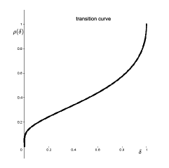
Figure 7: This figure illustrates the transition curve of Donoho and Tanner [13].

Supplementary material

We have already said that when $X$ is in general position the minimizer of problem (2) (resp. problem (3)) is unique. Concerning LASSO, a sketch of proof given in Tibshirani [32] shows the uniqueness of the LASSO estimator when $X$ is in general position. In order to provide a self-contained article, we show that when $X$ is in general position, the minimizer of problem (3) is unique when $R=0$ as well as when $R>0$. We have already stressed that when $\beta$ is identifiable with respect to the $\ell_{1}$ norm then $\beta$ is sparse. We show that when the identifiability holds for $\beta$ then the family $(X_{i})_{i\in{\rm supp}(\beta)}$ is linearly independent and thus the number of components of $\beta$ equal to 0 is larger than $p-n$. Finally, a proof that the stable nullspace property implies the identifiability condition is given

References

- [1] Rina Foygel Barber and Emmanuel J Candès. Controlling the false discovery rate via knockoffs. The Annals of Statistics, 43(5):2055–2085, 2015.
- [2] Mohsen Bayati and Andrea Montanari. The LASSO risk for Gaussian matrices. IEEE Transactions on Information Theory, 58(4):1997–2017, 2012.
- [3] Peter Bühlmann, Markus Kalisch, and Lukas Meier. High-dimensional statistics with a view toward applications in biology. 2014.
- [4] Peter Bühlmann and Sara van de Geer. Statistics for High-Dimensional Data: Methods, Theory and Applications. Springer, 2011.
- [5] Emmanuel Candes, Yingying Fan, Lucas Janson, and Jinchi Lv. Panning for gold: Model-x knockoffs for high-dimensional controlled variable selection. arXiv preprint arXiv:1610.02351, 2016.
- [6] Emmanuel J Candès, Yaniv Plan, et al. Near-ideal model selection by minimization. The Annals of Statistics, 37(5A):2145–2177, 2009.
- [7] Shaobing Chen and David Donoho. Basis pursuit. In Proceedings of 1994 28th Asilomar Conference on Signals, Systems and Computers, volume 1, pages 41–44. IEEE, 1994.
- [8] Ingrid Daubechies, Ronald DeVore, Massimo Fornasier, and C Sinan Güntürk. Iteratively reweighted least squares minimization for sparse recovery. Communications on pure and applied mathematics, 63(1):1–38, 2010.
- [9] Pascaline Descloux and Sylvain Sardy. Model selection with lasso-zero: adding straw to the haystack to better find needles. Journal of Computational and Graphical Statistics, pages 1–29, 2020.
- [10] Lee H Dicker. Variance estimation in high-dimensional linear models. Biometrika, 101(2):269–284, 2014.
- [11] David Donoho and Jared Tanner. Observed universality of phase transitions in high-dimensional geometry, with implications for modern data analysis and signal processing. Philosophical Transactions of the Royal Society A: Mathematical, Physical and Engineering Sciences, 367(1906):4273–4293, 2009.
- [12] David L Donoho and Michael Elad. Optimally sparse representation in general (nonorthogonal) dictionaries via minimization. Proceedings of the National Academy of Sciences, 100(5):2197–2202, 2003.
- [13] David L Donoho and Jared Tanner. Precise undersampling theorems. Proceedings of the IEEE, 98(6):913–924, 2010.
- [14] Charles Dossal, Marie-Line Chabanol, Gabriel Peyré, and Jalal Fadili. Sharp support recovery from noisy random measurements by -minimization. Applied and Computational Harmonic Analysis, 33(1):24–43, 2012.
- [15] Karl Ewald and Ulrike Schneider. On the distribution, model selection properties and uniqueness of the lasso estimator in low and high dimensions. Electronic Journal of Statistics, 14(1):944–969, 2020.
- [16] Simon Foucart and Holger Rauhut. A mathematical introduction to compressive sensing, volume 1. Springer, 2013.
- [17] Andrew Gelman and Francis Tuerlinckx. Type s error rates for classical and bayesian single and multiple comparison procedures. Computational Statistics, 15(3):373–390, 2000.
- [18] Caroline Giacobino, Sylvain Sardy, Jairo Diaz-Rodriguez, Nick Hengartner, et al. Quantile universal threshold. Electronic Journal of Statistics, 11(2):4701–4722, 2017.
- [19] Rémi Gribonval and Morten Nielsen. Sparse representations in unions of bases. IEEE Transactions on Information Theory, 49(12):3320–3325, 2003.
- [20] Jian Huang, Shuangge Ma, and Cun-Hui Zhang. Adaptive lasso for sparse high-dimensional regression models. Statistica Sinica, 18(4):1603, 2008.
- [21] Karim Lounici. Sup-norm convergence rate and sign concentration property of lasso and dantzig estimators. Electronic Journal of statistics, 2:90–102, 2008.
- [22] Nicolai Meinshausen and Peter Bühlmann. High-dimensional graphs and variable selection with the lasso. The Annals of Statistics, 34(3):1436–1462, 2006.
- [23] Nicolai Meinshausen and Bin Yu. Lasso-type recovery of sparse representations for high-dimensional data. The Annals of Statistics, 37(1):246–270, 2009.
- [24] Piotr Pokarowski, Wojciech Rejchel, Agnieszka Soltys, Michal Frej, and Jan Mielniczuk. Improving lasso for model selection and prediction. arXiv preprint arXiv:1907.03025, 2019.
- [25] Venkatesh Saligrama and Manqi Zhao. Thresholded basis pursuit: Lp algorithm for order-wise optimal support recovery for sparse and approximately sparse signals from noisy random measurements. IEEE Transactions on Information Theory, 57(3):1567–1586, 2011.
- [26] Ulrike Schneider and Patrick Tardivel. The geometry of uniqueness and model selection of penalized estimators including slope, lasso, and basis pursuit. arXiv preprint arXiv:2004.09106, 2020.
- [27] Matthew Stephens. False discovery rates: a new deal. Biostatistics, 18(2):275–294, 2017.
- [28] Weijie J Su, Małgorzata Bogdan, and Emmanuel J. Candès. False discoveries occur early on the lasso path. The Annals of Statistics, 45(5):2133–2150, 2017.
- [29] Patrick Tardivel. Représentation parcimonieuse et procédures de tests multiples: application à la métabolomique. PhD thesis, Université de Toulouse, Université Toulouse III-Paul Sabatier, 2017.
- [30] Patrick JC Tardivel, Rémi Servien, and Didier Concordet. Sparsest representations and approximations of an underdetermined linear system. Inverse Problems, 34(5):055002, 2018.
- [31] Robert Tibshirani. Regression shrinkage and selection via the lasso. Journal of the Royal Statistical Society. Series B (Methodological), 58(1):267–288, 1996.
- [32] Ryan J Tibshirani. The lasso problem and uniqueness. Electronic Journal of Statistics, 7:1456–1490, 2013.
- [33] Sara A Van de Geer. High-dimensional generalized linear models and the lasso. The Annals of Statistics, pages 614–645, 2008.
- [34] Sara A Van De Geer, Peter Bühlmann, et al. On the conditions used to prove oracle results for the lasso. Electronic Journal of Statistics, 3:1360–1392, 2009.
- [35] Martin J Wainwright. Sharp thresholds for high-dimensional and noisy sparsity recovery using constrained quadratic programming (lasso). IEEE transactions on information theory, 55(5):2183–2202, 2009.
- [36] S. Wang, H. Weng, and A. Maleki. Which bridge estimator is the best for variable selection ? arxiv, 2018.
- [37] Asaf Weinstein, Rina Barber, and Emmanuel J. Candès. A power and prediction analysis for knockoffs with lasso statistics. arXiv:1712.06465, 2017.
- [38] Asaf Weinstein, Weijie J Su, Małgorzata Bogdan, Rina F Barber, and Emmanuel J Candès. A power analysis for knockoffs with the lasso coefficient-difference statistic. arXiv preprint arXiv:2007.15346, 2020.
- [39] Peng Zhao and Bin Yu. On model selection consistency of lasso. The Journal of Machine Learning Research, 7:2541–2563, 2006.
- [40] Hui Zou. The adaptive lasso and its oracle properties. Journal of the American statistical association, 101(476):1418–1429, 2006.