Stochastic Gradient Descent for Spectral Embedding with Implicit Orthogonality Constraint

Abstract

In this paper, we propose a scalable algorithm for spectral embedding. The latter is a standard tool for graph clustering. However, its computational bottleneck is the eigendecomposition of the graph Laplacian matrix, which prevents its application to large-scale graphs. Our contribution consists of reformulating spectral embedding so that it can be solved via stochastic optimization. The idea is to replace the orthogonality constraint with an orthogonalization matrix injected directly into the criterion. As the gradient can be computed through a Cholesky factorization, our reformulation allows us to develop an efficient algorithm based on mini-batch gradient descent. Experimental results, both on synthetic and real data, confirm the efficiency of the proposed method in term of execution speed with respect to similar existing techniques.

1 Introduction

Graphs are appealing mathematical tools for modelling pairwise relationships between data points, without being limited by the rigid structure of Euclidean spaces. In a graph, the data points are represented as vertices, whereas the pairwise relationships between vertices are described by weighted edges. Examples of graph-based representations can be found in numerous application domains, such as biology, social networks, financial and banking, mobility and traffic patterns.

The main focus of this paper is spectral embedding, which aims at representing the nodes of a graph into a low-dimensional space that preserves the connectivity patterns described by the graph edges. In this regard, one of most popular approaches consists of embedding the graph vertices into a subspace spanned by the eigenvectors of the graph Laplacian matrix corresponding to the $K$ smallest eigenvalues [1, 2]. This leads to an optimization problem that can be solved by performing the eigendecomposition of the Laplacian matrix [3]. However, this technique may not scale well when the number of graph vertices grows big.

A possible way to reduce the computational requirements of eigendecomposition involves the use of Nyström method, a random sampling technique to approximate the eigenvectors of a large matrix [4]. Similarly, one can constrain the original eigendecomposition problem to satisfy the Nyström formula, so as to obtain a reduced-size problem that achieves a lower approximation error [5].

An alternative approach to speed up the computation of eigenvectors is to use the power method from the numerical linear algebra literature [6]. From an optimization viewpoint, the power method simultaneously updates all the coordinates of the iterate, but they converge to the optimal value at different speeds. Hence, it is possible to derive a coordinate-wise version of the power method for a further speedup [7].

Yet another direction to efficiently deal with spectral embedding involves the use of stochastic gradient optimization. The idea is to cast the algebraic problem of identifying the principal eigenvectors of a matrix as the optimization of a trace function subject to an orthogonality constraint [8, 9]. Therefore, a natural way to tackle this problem consists of using the notion of Riemannian gradients [10].

Contribution

In this work, we propose a stochastic optimization algorithm to deal with spectral embedding. Our main contribution consists of reformulating the latter so that the orthogonality constraint is replaced with an orthogonalization matrix in the criterion. As the gradient can be computed through a Cholesky factorization, our reformulation enables us to develop an efficient algorithm based on mini-batch gradient descent [11, 12]. The peculiarity of our approach is that the graph nodes are processed by splitting them in chunks of manageable size. This allows us to deal with much larger graphs than those tackled by similar methods [3, 10].

Outline

The paper is organized as follows. In Section 2, we formulate the spectral embedding problem. In Section 3, we describe the proposed reformulation and the stochastic gradient optimization algorithm to solve it. In Section 4, we compare our approach to similar spectral embedding methods. Finally, the conclusion is drawn in Section 5.

2 Problem formulation

In this paper, we aim at clustering a graph $\mathcal{G}(V,E,W)$ which consists of a set $V$ of vertices, and a set $E$ of edges with non-negative weights $w_{i,j}$, where $W=[w_{i,j}]_{i,j}\in\mathbb{R}^{N\times N}$ is the weighted adjacency matrix, with $w_{i,i}=0$ for all $i$.

The degree of a vertex $i$ in the graph $\mathcal{G}$, denoted as $d(i)$, is defined as the sum of weights of all the edges incident to $i$ in the graph $\mathcal{G}$. The degree matrix $D$ is then defined as

$$D_{i,j}=\begin{cases}d(i)\quad&\textup{if $i=j$}\\ 0\quad&\textup{otherwise.}\end{cases}$$ (1)

Based on $W$ and $D$, the Laplacian matrix of $\mathcal{G}$ is

$$L=D-W.$$ (2)

In the literature, $L$ is called the unormalized Laplacian matrix. There are also normalized versions of this matrix, such as

$$L_{\rm{sym}}=D^{-\frac{1}{2}}(D-W)D^{-\frac{1}{2}}.$$ (3)

The Laplacian matrix is of broad interest in the studies of spectral graph theory [13]. Although closely related to each other, the different definitions of the Laplacian matrix don’t enjoy the same properties. For example, $L$ and $L_{\rm{sym}}$ are both real and symmetric matrices, but they have a different set of eigenvalues and orthonormal eigenvectors. Moreover, each definition of the Laplacian matrix comes with its own algorithm to perform spectral embedding and clustering [14]. In this paper, we use the unnormalized graph Laplacian $L$ defined above, since its eigenvectors are orthonormal and its eigenvalues are non-negative, with the smallest equal to zero.

2.1 Spectral Clustering

Spectral clustering is a standard application of spectral embedding [15, 16, 14]. The idea is to represent the data points to be clustered as the vertices of a graph, whose edges describe the pairwise relationships between those points (e.g., computed with k-nearest neighbours). The core operation is to embed the graph vertices in a low-dimensional space, where the projected points can be trivially clustered. More specifically, for a $K$-way clustering, one aims at finding the semi-orthogonal matrix $U=\left[u_{1}\,|\dots|\,u_{N}\right]^{\top}$ such that its rows $u_{n}\in\mathbb{R}^{K}$ minimize the pairwise distances on the graph edges, namely

$$\operatorname*{minimize}_{U\in\mathbb{R}^{N\times K}}\;\;\operatorname{Tr}(U^{\top}LU):=\sum_{i=1}^{N}\sum_{j=1}^{N}w_{i,j}\|u_{i}-u_{j}\|^{2}$$

$$\quad{\rm s.t.}\quad U^{\top}U={\bf I_{K\times K}}.$$ (4)

Each row of the matrix $U$ is a point in the low-dimensional space $\mathbb{R}^{K}$ representing a graph vertex. Strongly-connected vertices are thus mapped to close vectors in $\mathbb{R}^{K}$. One can apply a $K$-mean algorithm on the rows of the solution $\bar{U}$, so that $K$ clusters are formed by grouping together the vertices that are the most strongly connected by the graph.

3 Proposed algorithm

It is well known that the solution to Problem (2.1) is the matrix formed by the eigenvectors associated to the $K$ smallest eigenvalues of the Laplacian matrix $L$. While there exist many efficient algorithms for spectral embedding [3, 4, 6, 5, 7, 10], they may not always scale well as the graph size $N$ grows big. Therefore, we propose an alternative approach to solve Problem (2.1), which consists of reformulating the latter so that it can be dealt with a stochastic optimization algorithm, such as mini-batch gradient descent [11, 12].

3.1 Forward-backward splitting

The main difficulty in solving Problem (2.1) via gradient descent arises from the orthogonality constraint. A possible way to circumvent this issue is to make use of forward-backward splitting [17], which boils down to the following iterations:

$$(\forall t\in\mathbb{N})\qquad U_{t+1}={\sf QR}\Big{(}U_{t}-\gamma_{t}LU_{t}\Big{)}.$$ (5)

Hereabove, $LU$ is the gradient of $\frac{1}{2}{\rm Tr}(U^{\top}LU)$, whereas the operator ${\sf QR}(\cdot)$ extracts the semi-orthogonal matrix $Q$ obtained with the QR decomposition of $U_{t}-\gamma_{t}LU_{t}$. Indeed, any rectangular matrix $U\in\mathbb{R}^{N\times K}$ with $N\geq K$ can be factorized as $U=QR$, where $Q\in\mathbb{R}^{N\times K}$ is semi-orthogonal, and $R\in\mathbb{R}^{K\times K}$ is upper triangular. This was the approach followed in [10], where a Riemannian gradient was used instead of the regular gradient.

3.2 Reformulation with implicit constraint

We propose an alternative approach to deal with the orthogonality constraint in Problem (2.1). Indeed, the latter can be enforced implicitly by using the upper triangular matrix $R$ of the QR decomposition of $U$, which is defined as

$$U=QR.$$ (6)

When $U$ is positive definite, the QR decomposition is unique, and $R$ is equal to the upper triangular factor of the Cholesky decomposition $U^{\top}U=R^{\top}R$. Then, it is possible to extract the Q-factor of $U$ as

$$Q=UR^{-1}.$$ (7)

This equality allows us to reformulate Problem (2.1) as

$$\operatorname*{minimize}_{U\in\mathbb{R}^{N\times K}}\;\;J(U):={\rm Tr}\Big{(}(UR^{-1})^{\top}L(UR^{-1})\Big{)}.$$ (8)

Note that the matrix $U$ is not semi-orthogonal, but $UR^{-1}$ is. Also, $R$ is a function of $U$, for which we can compute the gradient w.r.t. $U$ [18]. Therefore, the reformulated problem can be solved using standard gradient descent, yielding

$$(\forall t\in\mathbb{N})\qquad U_{t+1}=U_{t}-\gamma_{t}\nabla J(U_{t}).$$ (9)

3.3 Stochastic gradient descent

The main advantage in solving Problem (8) is that we can modify the update in Eq. (9) by replacing the function $J$ with a stochastic approximation $J_{t}$, yielding

$$(\forall t\in\mathbb{N})\qquad U_{t+1}=U_{t}-\gamma_{t}\nabla J_{t}(U_{t}).$$ (10)

Before we can define the above function $J_{t}$, let us denote by $\mathcal{I}$ the set of indexes associated to the nonzero elements in the upper triangular part of Laplacian matrix $L$, namely

$$\mathcal{I}=\Big{\{}(i,j)\in\{1,\dots,N\}^{2}\;|\;w_{i,j}\neq 0\;{\rm and}\;j>i\Big{\}}.$$ (11)

The Laplacian matrix can be thus decomposed as follows

$$L=\sum_{(i,j)\in\mathcal{I}}\underbrace{w_{i,j}\big{(}e_{i}e_{i}^{\top}+e_{j}e_{j}^{\top}-e_{i}e_{j}^{\top}-e_{j}e_{i}^{\top}\big{)}}_{\mathsf{L}_{i,j}\in\mathbb{R}^{N\times N}},$$ (12)

where $e_{n}$ is the $n$-th column of the $N\times N$ identity matrix. Thus, the original criterion in Problem (2.1) can be rewritten as

$$\operatorname{Tr}(U^{\top}LU)=\sum_{(i,j)\in\mathcal{I}}\operatorname{Tr}(U^{\top}\mathsf{L}_{i,j}U)=\sum_{(i,j)\in\mathcal{I}}w_{i,j}\|u_{i}-u_{j}\|^{2}.$$ (13)

To build the function $J_{t}$ appearing in Eq. (10), at every iteration $t$ we select a subset of indexes

$$\mathcal{S}_{t}\subset\mathcal{I},$$ (14)

we use those indexes to build a partial Laplacian matrix

$$\mathbf{L}_{t}=\sum_{(i,j)\in\mathcal{S}_{t}}\mathsf{L}_{i,j},$$ (15)

and we approximate the criterion in Eq. (8) as

$$J_{t}(U):={\rm Tr}\Big{(}(UR^{-1})^{\top}\mathbf{L}_{t}(UR^{-1})\Big{)}.$$ (16)

Here is where the proposed reformulation comes into play. As the term $\mathbf{L}_{t}$ contains many rows/columns filled with zeros, we never have to work with the full-size matrix $U$. Specifically, the function $J_{t}(U)$ boils down to

$$J_{t}(U):=\sum_{(i,j)\in\mathcal{S}_{t}}w_{i,j}\|(u_{i}-u_{j})^{\top}R^{-1}\|^{2}.$$ (17)

As for the Cholesky decomposition $U^{\top}U=R^{\top}R$, we compute the full-size matrix product at the algorithm initialization

$$M_{0}=U_{0}^{\top}U_{0}.$$ (18)

Since the update in Eq. (10) only modifies the terms $u_{i}$ and $u_{j}$ such that $(i,j)\in\mathcal{S}_{t}$, we can efficiently update it as

$$M_{t+1}=M_{t} +\sum_{(i,j)\in\mathcal{S}_{t}}\big{(}u_{i,t+1}u_{i,t+1}^{\top}-u_{i,t}u_{i,t}^{\top}\big{)}$$

$$+\sum_{(i,j)\in\mathcal{S}_{t}}\big{(}u_{j,t+1}u_{j,t+1}^{\top}-u_{j,t}u_{j,t}^{\top}\big{)}.$$ (19)

Putting all together, we arrive at the proposed optimization algorithm, which can be readily implemented with modern tools for automatic differentiation [19].

4 Numerical results

We evaluate the proposed algorithm in the context of multilayer graph clustering. An overview is given in the following.

4.1 Multilayer Graph Clustering

With the increasing richness of datasets, applications even rely often on multiple sources of information to characterize the relationships between data points. This leads to multi-layer graph representations, where data points are modelled as nodes shared across the layers, each of which describes a set of relationships (graph edges) on their set of observations (shared graph nodes). For example, a social network can be represented by a multilayer graph, where each layer corresponds to a different type of relationship among the same group of persons, such as friendships, music interests, etc.

More precisely, a multilayer graph consists of $S$ edge layers sharing the same vertices. Each layer $s$ is represented by a Laplacian matrix $L^{s}$, along with a spectral embedding matrix $U^{s}$ obtained as the solution to Problem (2.1). These matrices $(L^{s},U^{s})_{1\leq s\leq S}$ can be merged into a representative embedding matrix $U$ via the minimization of the projection distance in a Grassman manifold, defined as

$$d_{\sf proj}(U,\{U^{s}\}_{1\leq s\leq S})=KS-\sum_{s=1}^{S}\operatorname{Tr}\big{(}UU^{\top}U^{s}{U^{s}}^{\top}\big{)}.$$ (20)

Consequently, multilayer graph clustering boils down to [21]

$$\operatorname*{minimize}_{U\in\mathbb{R}^{N\times K}}\;\operatorname{Tr}\Big{(}\sum_{s=1}^{S}U^{\top}\big{(}L^{s}- \alpha\,U^{s}{U^{s}}^{\top}\big{)}U\Big{)}$$

$$\quad{\rm s.t.}\quad U^{\top}U={\bf I_{K\times K}}.$$ (21)

This is equivalent to perform spectral embedding on the aggregated Laplacian matrix defined as

$$L_{\sf MLG}=\sum_{s=1}^{S}(L^{s}-\alpha\,U^{s}{U^{s}}^{\top}),$$ (22)

where $\alpha>0$ is a regularization parameter.

For the sake of completeness, note that there exist other approaches to deal with a multilayer graph, such as averaging the Laplacian matrices of individual layers [22, 23, 24], or treating them as points in a Grassmann manifold [25, 26, 27, 21].

4.2 Datasets

In our experiments, we consider a synthetic dataset, as well as a real dataset coming from the Yelp challenge. Both have a multilayer graph representation of data.

As for the synthetic data, we consider a multilayer graph with $S=3$ layers and $K=5$ clusters. Data points are drawn from a Gaussian mixture model with five components, each representing a cluster. The goal with this dataset is to recover the five clusters of the graph vertices, using the layers constructed from the point clouds.

Yelp is a popular website for reviewing and rating local businesses. In our experiments, we only extract star ratings, text reviews, and review evaluations (users can mark reviews as “cool”, “useful”, and “funny”), ignoring the other information in the dataset. An example is shown in Fig. 1. Our goal is to cluster the businesses by predicting their ratings ($K=3$).

To build a multilayer graph on Yelp data, we proceed as follows. We preprocess the text reviews using sentiment analysis. This yields a polarity score within the range $[-1,1]$ on which we build a 5-nearest neighbor (NN) graph. We also build a 5-NN graph on the other features (“cool”, “useful”, and “funny” evaluations), leading to $S=4$ graph layers.

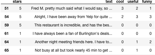
Figure 1: Yelp data before the preprocessing of text reviews.

4.3 Comparisons

We compare spectral embedding algorithms on Problem (4.1), assuming that the aggregated Laplacian matrix defined in Eq. (22) is given as input. This means that a spectral embedding problem is solved to compute each matrix $U^{s}$. For brevity, these problems are not considered into our analysis.

Problem setting

We evaluate the performance of three spectral embedding algorithms: matrix eigendecomposition [3], stochastic forward-backward splitting [10], and our method described in Section 3.3. Note that “matrix eigendecomposition“ uses the normalized version of the aggregated Laplacian matrix. The normalization is important to obtain a good clustering performance. However, this causes the method to slow down considerably, which gives rise to the interest of considering alternative approaches. The other methods use the unnormalized Laplacian matrix.

Implementation details

All the experiments were conducted in Python/Numpy on a 40-core Intel Xeon CPU at 2.5 GHz with 128GB of RAM. As for the proposed method, we used a step-size $\gamma=10^{-3}$, and mini-batches of size $4^{\prime}000$. The latter is a critical parameter, as mini-batches should be big enough to capture the structure of the Laplacian matrix. For this reason, it is also highly important that mini-batches are sampled at random from the entire dataset at each step, and not be fixed across iterations.

Result analysis

We use three criteria to measure the clustering performance: Purity, Normalized Mutual Information (NMI), and Rand Index (RI). The results reported in Tables 1 and 2 for both synthetic and Yelp data show that the proposed method achieves almost the same clustering performance as the matrix eigendecomposition, while being faster than the other compared methods. The small differences in the performance are related to the stochastic nature of our optimization algorithm. Running it for less iterations would allow us to get even faster results, yet less accurate. There is thus a tradeoff between speed and accuracy, as usual in optimization.

Table 1: Clustering on synthetic data ($N=10^{\prime}000$).

Method	Time	Iter.	Purity	NMI	RI
Eigendecomp.	36.3 s	-	0.93	0.83	0.85
Stochastic FB	22.8 s	3000	0.94	0.84	0.86
Proposed	5.2 s	500	0.92	0.79	0.82

Table 2: Clustering on Yelp data ($N=11^{\prime}160$).

Method	Time	Iter.	Purity	NMI	RI
Eigendecomp.	69.7 s	-	0.87	0.65	0.56
Stochastic FB	50.6 s	3000	0.88	0.79	0.88
Proposed	11.4 s	500	0.86	0.71	0.84

5 Conclusion

In this paper, we proposed a reformulation of spectral embedding that allowed us to devise a new optimization algorithm based on stochastic gradient descent. The experimental results showed that the proposed approach is more efficient than matrix eigendecomposition and stochastic Riemannian optimization on medium-size datasets. This confirms that our approach is capable of scaling to larger datasets than what similar spectral embedding methods can handle.

There are a number of extensions that we are currently investigating, such as the possibility to extend our approach to the Riemann manifold of semi-positive definite matrices [28], and to simultaneously compute the embedding matrices of each layer and the aggregated graph. Moreover, a GPU implementation of the proposed algorithm is under development.

References

- [1] E. Schaeffer, “Survey: Graph clustering,” Computer Science Review, vol. 1, no. 1, pp. 27 – 64, Aug. 2007.
- [2] S. Fortunato, “Community detection in graphs,” Physics Reports, vol. 486, no. 3 – 5, pp. 75–174, Feb. 2010.
- [3] M. Belkin and P. Niyogi, “Laplacian eigenmaps for dimensionality reduction and data representation,” Neural Computation, vol. 15, no. 6, pp. 1373–1396, 2003.
- [4] C. Fowlkes, S. Belongie, F. Chung, and J. Malik, “Spectral grouping using the Nyström method,” IEEE Trans. Pattern Anal. Mach. Intell., vol. 26, pp. 214–225, 2004.
- [5] M. Vladymyrov and M. Carreira-Perpinan, “The variational Nyström method for large-scale spectral problems,” in Proceedings of ICML, New York, USA, June 2016, vol. 48, pp. 211–220.
- [6] C. Boutsidis, P. Kambadur, and A. Gittens, “Spectral clustering via the power method – provably,” in Proceedings of ICML, Lille, France, July 2015.
- [7] Q. Lei, K. Zhong, and I. S. Dhillon, “Coordinate-wise power method,” in Advances in Neural Information Processing Systems, pp. 2064–2072. 2016.
- [8] Q. Xu, M. DesJardins, and K. Wagstaff, “Constrained spectral clustering under a local proximty structure,” Proceedings of the 18th International Florida Artificial Intelligence Research Society, May 2005.
- [9] X. Wang and I. Davidson, “Flexible constrained spectral clustering,” Proc. of ACM SIGKDD, pp. 563–572, 2010.
- [10] Y. Han and M. Filippone, “Mini-batch spectral clustering,” in International Joint Conference on Neural Networks, May 14–19 2017, pp. 3888–3895.
- [11] S. J. Reddi, S. Kale, and S. Kumar, “On the convergence of adam and beyond,” in Proceedings of ICLR, Vancouver, Canada, May 2018.
- [12] V. Dudar, G. Chierchia, E. Chouzenoux, J.-C. Pesquet, and V. Semenov, “A two-stage subspace trust region approach for deep neural network training,” in Proceedings of EUSIPCO, Kos island, Greece, Sept. 2017.
- [13] F. R. K. Chung, “Spectral graph theory,” CBMS Regional Conference Series in Mathematics, American Mathematical Society, 1997.
- [14] U. von Luxburg, “A tutorial on spectral clustering,” Statistics and Computing, vol. 17, no. 4, pp. 395–416, 2007.
- [15] J. Shi and J. Malik, “Normalized cuts and image segmentation,” IEEE Transactions on Pattern Analysis and Machine Intelligence, vol. 22, no. 8, pp. 888–905, Aug. 2000.
- [16] A. Ng, M. Jordan, and Y. Weiss, “On spectral clustering: Analysis and an algorithm,” Advances in Neural Information Processing Systems, pp. 849–856, 2001.
- [17] P. L. Combettes and V. R. Wajs, “Signal recovery by proximal forward-backward splitting,” Multiscale Model. Sim., vol. 4, no. 4, pp. 1168–1200, 2005.
- [18] I. Murray, “Differentiation of the Cholesky decomposition,” Eprint arXiv:1602.07527, 2016.
- [19] A. Paszke, S. Gross, S. Chintala, G. Chanan, E. Yang, Z. DeVito, Z. Lin, A. Desmaison, L. Antiga, and A. Lerer, “Automatic differentiation in pytorch,” in Proceedings of the NIPS Workshop on Autodiff. 2017.
- [20] J. Hamm and D. D. Lee, “Grassmann discriminant analysis: A unifying view on subspace-based learning,” in Proceedings of ICML, Helsinki, Finland, 2008.
- [21] X. Dong, P. Frossard, P. Vandergheynst, and N. Nefedov, “Clustering on multi-layer graphs via subspace analysis on grassmann manifolds,” IEEE Transactions on Signal Processing, vol. 62, no. 4, pp. 905–918, 2014.
- [22] A. Argyriou, M. Herbster, and M. Pontil, “Combining graph laplacians for semi-supervised learning,” Advances in Neural Information Processing Systems, 2005.
- [23] L. Tang, X. Wang, and H. Liu, “Community detection via heterogeneous interaction analysis,” Data Min. Knowl. Discov., vol. 25, no. 1, pp. 1–33, Jul. 2012.
- [24] P.-Y. Chen and A. O. Hero, “Multilayer spectral graph clustering via convex layer aggregation: Theory and algorithms,” arXiv:1708.02620, 2017.
- [25] V. Sindhwani and P. Niyogi, “A co-regularization approach to semi-supervised learning with multiple views,” in ICML Workshop on Learning with Multiple Views, 2005.
- [26] A. Kumar and H. Daumé, “A co-training approach for multi-view spectral clustering,” in Proc. of ICML, 2011.
- [27] X. Wang, W. Bian, and D. Tao, “Grassmannian regularized structured multi-view embedding for image classification,” IEEE Transactions on Image Processing, vol. 22, no. 7, pp. 2646–2660, Jul. 2013.
- [28] M. El Gheche and P. Frossard, “Multilayer graph signal clustering,” Preprint arXiv: 1811.00821, 2018.