Network Coding with Random Packet-Index Assignment for Data Collection Networks

Abstract

This paper considers data collection using a network of uncoordinated, heterogeneous, and possibly mobile devices. Using medium and short-range radio technologies, multi-hop communication is required to deliver data to some sink. While numerous techniques from managed networks can be adapted, one of the most efficient (from the energy and spectrum use perspective) is network coding (NC). NC is well suited to networks with mobility and unreliability, however, practical NC requires a precise identification of individual packets that have been mixed together. In a purely decentralized system, this requires either conveying identifiers in headers along with coded information as in COPE, or integrating a more complex protocol in order to efficiently identify the sources (participants) and their payloads.

A novel solution, Network Coding with Random Packet Index Assignment (NeCoRPIA), is presented where packet indices in NC headers are selected in a decentralized way, by choosing them randomly. Traditional network decoding can be applied when all original packets have different indices. When this is not the case, i.e., in case of collisions of indices, a specific decoding algorithm is proposed. A theoretical analysis of its performance in terms of complexity and decoding error probability is described. Simulation results match well the theoretical results. Comparisons of NeCoRPIA header lengths with those of a COPE-based NC protocol are also provided.

I Introduction

In smart cities, smart factories, and more generally in modern Internet of Things (IoT) systems, efficient data collection networks (DCN) are growing in importance to gather various information related to the environment and the human activity [1]. This trend is accelerated by the development of a wide variety of objects with advanced sensing and connectivity capabilities, which offer the possibility to collect information of more diversified nature. This also leads to the emergence of new DCN modalities such as participatory sensing or crowdsensing applications [2], which contrast with classical DCN architectures, where nodes are owned and fully controlled by one managing authority.

To transmit data in DCN, various communication protocols may be considered, depending on the radio technology integrated in the sensing devices. Long- (4G, NB-IoT, 5G, LoRa, SigFox), medium- (WiFi), and short-range (ZigBee, Bluetooth) radio technologies and protocols have all their advantages and shortcomings [3].

One of the challenges with new DCN modalities is the distributed nature of the network with unpredictable stability, high churn rate, and node mobility. Here, one focuses on DCN scenarios where measurements from some area are collected using medium- or short-range radio technologies, which require multi-hop communication [4, 5, 6, 7, 8, 9]. For such scenarios, a suitable communication technique is Network Coding (NC) [10, 11, 12, 13, 14, 15]. NC [16] is a transmission paradigm for multi-hop networks, in which, rather than merely relaying packets, the intermediate nodes may mix the packets that they receive. In wireless networks, the inherent broadcast capacity of the channel improves the communication efficiency [17, 18, 19].

In practical NC (PNC) protocols, the mixing of the packets is achieved through linear combinations. The corresponding coding coefficients are generally included in each mixed packet as an encoding vector [20] (see Figure 1). In this way, a coefficient can be uniquely associated with the corresponding packet: the downside is the requirement for a global indexing of all packets in the network. When a single source generates and broadcasts network-coded packets (intra-flow NC) as in [19, 21], such indexing is easily performed, since the source controls the initial NC headers of all packets. When the packets of several sources are network coded together (inter-flow NC [22]), a global packet indexing is difficult to perform in a purely distributed system, where sources may appear, move, and disappear. This is also true when intra and inter-flow NC is performed [23].

Moreover, even in a static network of $N$ sensor nodes, each potentially generating a single packet, assuming that all packets may be NC together in some Galois field $\mathbb{F}_{q}$, headers of $N\log_{2}q$ bits would be required. In practice, only a subset of packets are NC together, either due to the topology of the network, or to constraints imposed on the way packets are network-coded [24, 11, 25]. This property allows NC headers to be compressed [24, 26, 27], but does not avoid a global packet indexing. This indexing issue has been considered in COPE [18], where each packet to be network coded is identified by a 32-bit hash of the IP source address and IP sequence number. Such solution is efficient when few packets are coded, but leads to large NC headers when the number of coded packets increases.

The major contribution of this paper is Network Coding with Random Packet-Index Assignment (NeCoRPIA), an alternative approach to COPE, addressing global packet indexing, while keeping relatively compact NC headers. With NeCoRPIA, packet indices in NC headers are selected in a decentralized way, by simply choosing them randomly. In dynamic networks, NeCoRPIA does not require an agreement among the nodes on a global packet indexing. In a DCN, when packets generated by a small proportion of nodes have to be network coded, with NeCoRPIA, NC headers of a length proportional to the number of nodes generating data are obtained.

This paper reviews some related work in Section II. Section III presents the architecture and protocol of NeCoRPIA, our version of PNC dedicated to data collection. Section IV describes network decoding techniques within the NeCoRPIA framework. Section V analyzes the complexity of the proposed approach. Section VI evaluates the performance of NeCoRPIA in terms of decoding error. Section VII provides simulations of a DCN to compare the average header length of NeCoRPIA with plain NC and with a COPE-inspired approach. Finally, Section VIII provides some conclusions and future research directions.

II Related Work

The generic problem of efficiently collecting information from multiple sources to one or several sinks in multi-hop networks has been extensively studied in the literature: for instance, for static deployments of wireless sensor networks, a routing protocol such as the Collection Tree Protocol (CTP) [28] is typical. Focusing on the considered data collection applications [2], performance can be improved by the use of NC, as exemplified by [17] where NC is shown to outperform routing in a scenario with multiple sources (all-to-all broadcast) or by [11, 12, 14], where NC is employed for data collection in a sensor network, see also [5, 6, 8]. Combinations of NC and opportunistic routing have also been considered, see [29] and the references therein.

NeCoRPIA addresses two issues related to the use of NC in DCN, namely the need for a global packet indexing and the overhead related to NC headers.

An overview of NC header compression techniques has been provided in [27]. For example, [30] explores the trade-off between field size and generation (hence encoding vector) size. In [24, 31], encoding vectors are compressed using parity-check matrices of channel codes yielding gains when only limited subsets of linear combinations are possible. In [26] a special coding scheme permits to represent NC headers with one single symbol at the expense of limited generation sizes. In Tunable Sparse NC (TNSC) [25, 32], COPE-inspired headers are used and the sparsity level of NC headers is optimized by controlling the number of network-coded packets. Similar results may also be obtained by a dynamic control of the network topology as proposed in [15]. In Fulcrum NC [33], $g$ packets generated by a source are first encoded using a channel code over some extension field, e.g., $\mathbb{F}_{2^{8}}$, using a (systematic) Reed-Solomon code to generate $r$ redundancy packets. The $g+r$ packets are then network coded over $\mathbb{F}_{2}$. Powerful receivers may retrieve the $g$ original packet from $g$ independent linear combinations seen as mixtures over the extension field, whereas limited receivers require $g+r$ independent combinations to be decoded over $\mathbb{F}_{2}$. NC headers of $g+r$ bits are thus necessary. Nevertheless, this approach does not address the global packet indexing issue and is better suited to intra-flow NC.

Going further, the encoding vectors may be entirely removed from the header of packets. Network decoding may then be seen as a source separation problem using only information about the content of packets. Classical source separation aims at recovering source vectors defined over a field (e.g., $\mathbb{R}$ or $\mathbb{C}$) from observations linearly combined through an unknown encoding matrix [34]. In $\mathbb{R}$, one classical approach to source separation is Independent Component Analysis (ICA) [34], which estimates the sources as the set of linear combinations that minimizes the joint entropy and the mutual similarity among vectors. In previous work, we have proposed different techniques that exploit ICA over finite fields [35] in the context of NC. In [36], network-coded packets without encoding vectors are decoded using entropy minimization jointly with channel encoding, while in [37], we exploit the redundancy introduced by communication protocols to assist the receiver in decoding. The price to pay is a significantly larger decoding complexity compared to simple Gaussian elimination when considering classical NC, which prohibits considering large generation sizes.

When packets from several sensor nodes have to be network coded, employing the format of NC vectors proposed by [20] requires a coordination among nodes. This is necessary to avoid two nodes using the same encoding vector when transmitting packets. Figure 1 (left) shows four sensor nodes, each generating a packet supplemented by a NC header, which may be seen as a vector with entries in the field $\mathbb{F}$ in which NC operations are performed. A different base vector is chosen for each packet to ensure that packets can be unmixed at receiver side. The coordination among nodes is required to properly choose the number of entries in $\mathbb{F}$ that will build up the NC header and the allocation of base vectors among nodes.

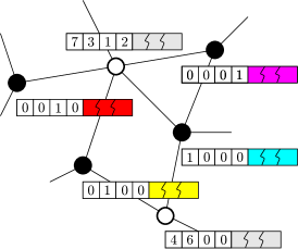
Figure 1: NC headers as proposed by [20] (left), by [18] (middle) and NeCoRPIA NC headers (with $n_{\text{v}}=1$) (right) in the case of inter-session coding of packets generated by different sensor nodes; nodes generating data packets are in black and nodes relaying packets are in white

COPE [18] or TSNC [25] employ a header format including one identifier (32-bit hash for COPE) for each of the coded packets, see Figure 1 (middle). When several packets are network coded together, their identifier and the related NC coefficient are concatenated to form the NC header. There is no more need for coordination among nodes and the size of the NC header is commensurate with the number of mixed packets. Nevertheless, the price to be paid is a large increase of the NC header length compared to a coordinated approach such as that proposed in [20].

To the best of our knowledge, NeCoRPIA represents the only alternative to COPE to perform a global packet indexing in a distributed way, allowing packets generated by several uncoordinated sources to be efficiently network coded. A preliminary version of NeCoRPIA was first presented in [38], where a simple random NC vector was considered, see Figure 1 (right). Such random assignment is simple, fast, and fully distributed but presents the possibility of collisions, that is, two packets being assigned to the same index by different nodes. Here, we extend the idea in [38], by considering a random assignment of several indexes to each packet. This significantly reduces the probability of collision compared to a single index, even when represented on the same number of bits as several indexes. Since collisions cannot be totally avoided, an algorithm to decode the received packets in spite of possible collisions is also proposed. We additionally detail how this approach is encompassed in a practical data collection protocol.

III NeCoRPIA Architecture and Protocol

III-A Objective of the data collection network

A data collection architecture is considered with a set $\mathcal{S}=\{S_{1},\ldots,S_{N}\}$ of $N$ static nodes gathering measurements performed by possibly mobile sensing nodes. Each node $S_{i}$, located in $\boldsymbol{\theta}_{i}$, in some reference frame $\mathcal{F}$, acts as a data collection point for all mobile nodes located in its assigned area $\mathcal{R}_{i}$ (e.g., its Voronoi cell) as in Figure 2. The data consist, for instance, in a set of measurements of some physical quantity $D(\boldsymbol{\xi})$, e.g., temperature, associated with the vector $\boldsymbol{\xi}$, representing the experimental conditions under which the measurements were taken (location, time instant, regressor vector in case of model linear in some unknown parameters). Note that for crowdsensing applications, the identity of the node that took the measurements is often secondary, provided that there are no node polluting the set of measurements with outliers.

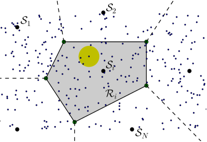
Figure 2: Data collection scenario: the static node $S_{i}$ gathers measurements from all mobile nodes (with limited communication range) in its assigned data collection area $\mathcal{R}_{i}$ in grey

Typically, a mobile node measures periodically $D$ under the experimental conditions $\boldsymbol{\xi}$. The data collection network objective is to collect the tuples $(\boldsymbol{\xi},\mathbf{d})$, where $\mathbf{d}=D(\boldsymbol{\xi})$, to the appropriate collection point $S_{i}$ (responsible for the area $\mathcal{R}_{i}$ where the mobile node finds itself).

III-B General Architecture

For fulfilling the objectives of the previous section, a communication architecture based on NC is designed where information is propagated to the closest sink through dissemination of coded packets.

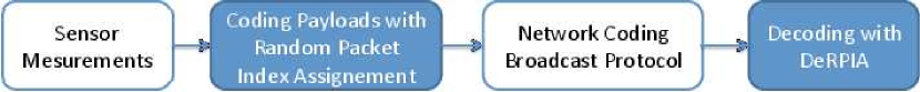
Figure 3: Modules of NeCoRPIA architecture

Figure 3 represents the modules involved in NeCoRPIA. The sensing module is in charge of collecting local sensor information with associated experimental conditions, i.e., the tuple $\left(\boldsymbol{\xi},\mathbf{d}\right)$. The encoding module takes as input $\left(\boldsymbol{\xi},\mathbf{d}\right)$ and creates packets containing the data payload, and our specific NeCoRPIA header. The NC protocol aims at ensuring that all (coded) packets reach the collection points, by transmitting at intermediate nodes (re)combinations of received packets. The decoding module at the collection points applies the algorithm from Section IV to recover the experimental data collected in the considered area $\mathcal{R}_{i}$.

III-C Network Encoding Format

Figure 4 represents the general packet format used in NeCoRPIA: it includes a control header used by the NC dissemination protocol, followed by an encoded content, considered as symbols from $\mathbb{F}_{q}$, the Galois field with $q$ elements.

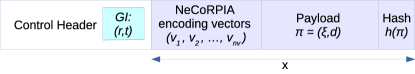
Figure 4: NeCoRPIA packet format

The control header itself includes, as generation identifier (GI), a spatio-temporal slot (STS) $\left(r,t\right)$, where $r$ is the index of the sink $\mathcal{S}_{r}$ and $t$ is the index of the considered time slot, within which the data has been collected. Only packets with the same GI are combined together by the protocol. The rest of the packet can be formally written as a vector $\mathbf{x}$ of $L_{\text{x}}$ entries in $\mathbb{F}_{q}$ as

$$\mathbf{x}=\left(\mathbf{v}_{1},\dots,\mathbf{v}_{n_{\text{v}}},\mathbf{\boldsymbol{\pi}},\mathbf{h}\right),$$ (1)

where $\mathbf{v}_{\ell}\in\mathbb{F}_{q}^{L_{\ell}}$, $\ell=1,\dots,n_{\text{v}}$ represent the encoding subvectors, $\mathbf{\boldsymbol{\pi}}=(\boldsymbol{\xi},\mathbf{d})$ is the payload, where $\boldsymbol{\xi}$ and $\mathbf{d}$ are represented with finite precision on a fixed number $L_{\mathbf{\boldsymbol{\pi}}}$ of symbols in $\mathbb{F}_{q}$, and $\mathbf{h}=h(\mathbf{\boldsymbol{\pi}})\in\mathbb{F}_{q}^{L_{\text{h}}}$ is the hash of $\mathbf{\boldsymbol{\pi}}$. In classical NC, $n_{\text{v}}=1$, and $\mathbf{v}_{1}$ corresponds to one of the canonical vectors of $\mathbb{F}_{q}^{L_{1}}.$ The choice of the canonical vector requires an agreement among mobile sensing nodes, to avoid the same vector being selected by two or more mobile nodes in the same STS.

To avoid this resource-consuming agreement step, when a source generates a packet, NeCoRPIA assigns random canonical vectors $\mathbf{e}_{i}\in\mathbb{F}_{q}^{L_{\ell}}$ to each $\mathbf{v}_{\ell}$, $\ell=1,\dots,n_{\text{v}}$. For each new payload $\mathbf{\boldsymbol{\pi}}$, the random NC vector is then represented by $\left(\mathbf{v}_{1},\dots,\mathbf{v}_{n_{\text{v}}}\right)$. One may choose $n_{\text{v}}=1$, but in this case, $L_{1}$ should be quite long to avoid collisions, even for a moderate number of packets in each STS (this is reminiscent to the birthday paradox [39]), see Section V-E1. This results in an encoding vector with the format represented in Figure 4 for the case $n_{\text{v}}=1$.

The hash $\mathbf{h}$ is included to assist the decoding process in case of collisions.

III-D Network Coding Protocol

The NC protocol is in charge of ensuring that the coded packets are properly reaching the data collection points for later decoding. Since the main contribution of our method lies in other parts, we only provide the sketch of a basic protocol. It operates by broadcasting measurements to all nodes within each area $\mathcal{R}_{i}$, with NC (in the spirit of [17]): with the effect that the collection point $S_{i}$ will gather the information as well. It is a multi-hop protocol relying on the control header, shown in Figure 4, to propagate control information to the entire network (as DRAGONCAST [40] does for instance). The control headers are generated by the data collection points and copied in each encoded packet by the nodes.

The baseline functioning is as follows: at the beginning of each STS, $S_{i}$ initiates data collection by generating packets with an empty payload, and with a source control header holding various parameters such as: number of encoding subvectors $n_{\text{v}}$ and size of each encoding vector $L_{\ell}$, $\ell=1,\dots,n_{\text{v}}$, the buffer size $G_{B}$, the STS $(r,t)$, along with a compact description of its area $\mathcal{R}_{i}$, sensing parameters, etc. Upon receiving packets from a data collection point or from other nodes, and as long its current position matches $\mathcal{R}_{i}$, a node periodically retransmits (coded) packets with the most up-to-date control header. When several measurements are taken within the same STS, packets with different random encoding vectors should be generated. Furthermore, each node maintains a buffer of (at most) $G_{B}$ coded vectors: when a packet associated to a given STS is received, it is (linearly) combined with all coded packets associated with the same STS in the buffer. Likewise, when a packet is generated in some STS, the node computes a linear combination of all coded packets belonging to the same STS and stored in the buffer. $S_{i}$ (indirectly) instructs nodes to stop recoding of packets of a STS (and to switch to the next one) through proper indication in the control header. Note that many improvements of this scheme exist or can be designed.

IV Estimation of the transmitted packets

Assume that within a STS $\left(r,s\right)$, mobile sensing nodes have generated a set of packets $\mathbf{x}_{1},\ldots,\mathbf{x}_{g}$, which may be stacked in a matrix $\mathbf{X}$. Assume that $g^{\prime}\geqslant g$ linear combinations of the packets $\mathbf{x}_{1},\ldots,\mathbf{x}_{g}$ are received by the data collection point $\mathcal{S}_{r}$ and collected in a matrix $\mathbf{Y}^{\prime}$ such that

$$\mathbf{Y}^{\prime}=\mathbf{A}^{\prime}\mathbf{X}=\mathbf{A}^{\prime}\left(\mathbf{V}_{1},\dots,\mathbf{V}_{n_{\text{v}}},\mathbf{P}\right),$$ (2)

where $\mathbf{A}^{\prime}$ represents the NC operations that have been performed on the packets $\mathbf{x}_{1},\ldots,\mathbf{x}_{g}$. $\mathbf{V}_{1},\dots,\mathbf{V}_{n_{\text{v}}}$, and $\mathbf{P}$ are matrices which rows are the corresponding vectors $\mathbf{v}_{1,i},\dots,\mathbf{v}_{n_{\text{v}},i}$, and $\mathbf{p}_{i}=\left(\boldsymbol{\pi}_{i},\mathbf{h}_{i}\right)\in\mathbb{F}_{q}^{L_{\mathbf{p}}}$ of the packets $\mathbf{x}_{i}$, $i=1,\dots,g$, with $L_{\text{p}}=L_{\mathbf{\boldsymbol{\pi}}}+L_{\text{h}}$. If enough linearly independent packets have been received, a full-rank $g$ matrix $\mathbf{Y}$ may be extracted by appropriately selecting $g$ rows of $\mathbf{Y}^{\prime}$. The corresponding $g$ rows of $\mathbf{A}^{\prime}$ form a $g\times g$ full-rank matrix $\mathbf{A}$. Then, (2) becomes

$$\mathbf{Y}=\mathbf{A}\left(\mathbf{V}_{1},\dots,\mathbf{V}_{n_{\text{v}}},\mathbf{P}\right).$$ (3)

The problem is then to estimate the packets $\mathbf{x}_{1},\ldots,\mathbf{x}_{g}$ from the received packets in $\mathbf{Y}$, without knowing $\mathbf{A}$.

Three situations have to be considered. The first is when the rows of $\left(\mathbf{V}_{1},\dots,\mathbf{V}_{n_{\text{v}}}\right)$ are linearly independent due to the presence of some $\mathbf{V}_{\ell}$ of full rank $g$. The second is when the rows of $\left(\mathbf{V}_{1},\dots,\mathbf{V}_{n_{\text{v}}}\right)$ are linearly independent but there is no full rank $\mathbf{V}_{\ell}$. The third is when the rank of $\left(\mathbf{V}_{1},\dots,\mathbf{V}_{n_{\text{v}}}\right)$ is strictly less than $g$, but the rank of $\mathbf{Y}$ is equal to $g$. These three cases are illustrated in Examples 1-3. In the last two situations, a specific decoding procedure is required, which is detailed in Section IV-B.

Example 1.

Consider a scenario where three nodes generate packets with $n_{\text{v}}=2$ random coding subvectors in $\mathbb{F}_{2}^{L_{\ell}}$ with $L_{1}=L_{2}=3$. When the generated coding vectors are $\left(\left(1,0,0\right),\left(0,1,0\right)\right)$, $\left(\left(1,0,0\right),\left(0,0,1\right)\right)$, and $\left(\left(0,0,1\right),\left(1,0,0\right)\right)$, two nodes have selected the same first coding subvector, but all second coding subvectors are linearly independent, which allows one to recover the original packets via Gaussian elimination. This situation is illustrated in Figure 5 ($a$), where each coding vector may be associated to a point in a $3\times 3$ grid, the first coding vector representing the row index and the second coding subvector the column index. Three different columns have been selected, decoding can be performed via Gaussian elimination on the second coding subvectors.

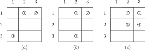
Figure 5: ($a$) Illustration of Example 1: No collision in the second subvectors; ($b$) Illustration of Example 2: single collisions in both subvectors; ($c$) Illustration of Example 3: single collisions in both subvectors leading to a cycle and a rank deficiency.

Example 2.

Consider the same scenario as in Example 1. When the generated coding vectors are $\left(\left(1,0,0\right),\left(0,1,0\right)\right)$, $\left(\left(1,0,0\right),\left(0,0,1\right)\right)$, and $\left(\left(0,0,1\right),\left(0,1,0\right)\right)$, collisions are observed in the first and second coding subvectors, but $\left(\mathbf{V}_{1},\mathbf{V}_{2}\right)$ is of full rank $g=3$. This situation is illustrated in Figure 5 ($b$): three different entries have been chosen randomly, decoding will be easy.

Example 3.

Consider now a scenario where four nodes generate packets with $n_{\text{v}}=2$ random coding subvectors in $\mathbb{F}_{2}^{L_{\ell}}$ with $L_{1}=L_{2}=3$. When the randomly generated coding vectors are $\left(\left(1,0,0\right),\left(0,1,0\right)\right)$, $\left(\left(1,0,0\right),\left(0,0,1\right)\right)$, $\left(\left(0,1,0\right),\left(0,1,0\right)\right)$, and $\left(\left(0,1,0\right),\left(0,0,1\right)\right)$, the rank of $\left(\mathbf{V}_{1},\mathbf{V}_{2}\right)$ is only three. $\mathbf{Y}$ will be of full rank $g=4$ only if $\left(\mathbf{V}_{1},\mathbf{V}_{2},\mathbf{P}\right)$ is of full rank. This situation is illustrated in Figure 5 ($c$): even if different entries have been chosen, the rank deficiency comes from the fact that the chosen entries may be indexed in such a way that they form a cycle.

IV-A Decoding via Gaussian elimination

When $\mathbf{A}$ is a $g\times g$ full-rank matrix, a necessary and sufficient condition to have the rank of one of the matrices $\mathbf{AV}_{\ell}$ equal to $g$ is that all mobile sensing nodes have chosen a different canonical subvector for the component $\mathbf{v}_{\ell}$ of the NC vector. Decoding may then be performed via usual Gaussian elimination on $\mathbf{AV}_{\ell}$, as in classical NC. As will be seen in Section VI, this event is unlikely, except for large values of $L_{\ell}$ compared to the number of packets $g$.

IV-B Decoding with packet index collisions

When $\mathbf{A}$ is a $g\times g$ full-rank matrix, the rank of $\mathbf{AV}_{\ell}$ is strictly less than $g$ when at least two rows of $\mathbf{V}_{\ell}$ are identical, i.e., two nodes have chosen the same canonical subvector. This event is called a collision in the $\ell$-th component of the NC vector.

When $\mathbf{A}$ is a $g\times g$ full-rank matrix, the rank of $\mathbf{A}\left[\mathbf{V}_{1},\dots,\mathbf{V}_{n_{\text{v}}}\right]$ is strictly less than $g$ when the rows of $\left[\mathbf{V}_{1},\dots,\mathbf{V}_{n_{\text{v}}}\right]$ are linearly dependent. This may obviously occur when the NC vector chosen by two nodes are identical, i.e., there is a collision in all $n_{\text{v}}$ components of their NC vector. This also occurs when there is no such collision, when nodes have randomly generated linearly dependent NC subvectors, as illustrated in Example 3, see also Section V.

IV-B1 Main idea

In both cases, one searches a full rank matrix $\mathbf{W}$ such that $\mathbf{X=W}\mathbf{Y}$ up to a permutation of the rows of $\mathbf{X}$. We propose to build this unmixing matrix $\mathbf{W}$ row-by-row exploiting the part of the packets containing the $n_{\text{v}}$ NC subvectors $\left(\mathbf{A}\mathbf{V}_{1},\dots,\mathbf{\mathbf{A}V}_{n_{\text{v}}}\right)$, which helps defining a subspace in which admissible rows of $\mathbf{W}$ have to belong. Additionally, one exploits the content of the packets and especially the hash $h\left(\boldsymbol{\pi}\right)$ introduced in Section III-C to eliminate candidate rows of $\mathbf{W}$ leading to inconsistent payloads.

IV-B2 Exploiting the collided NC vectors

For all full rank $g$ matrix $\mathbf{Y}$, there exists a matrix $\mathbf{T}$ such that $\mathbf{TY}$ is in reduced row echelon form (RREF)

$$\mathbf{T}\mathbf{Y}=\left(\begin{array}[]{ccccc}\mathbf{B}_{11}&\mathbf{B}_{12}&&\mathbf{B}_{1n_{\text{v}}}&\mathbf{C}_{1}\\ \mathbf{0}&\mathbf{B}_{22}\\ \mathbf{0}&\mathbf{0}&\ddots&&\vdots\\ \vdots&&\ddots&\mathbf{B}_{n_{\text{v}}n_{\text{v}}}\\ \mathbf{0}&\cdots&\cdots&\mathbf{0}&\mathbf{C}_{n_{\text{v}}+1}\end{array}\right),$$ (4)

where $\mathbf{B}_{\ell\ell}$ is a $\rho_{\ell}\times L_{\ell}$ matrix with $\text{rank}\left(\mathbf{B}_{\ell\ell}\right)=\rho_{\ell}$. Since $\textrm{rank}\left(\mathbf{Y}\right)=g$, $\mathbf{C}_{n_{\text{v}}+1}$ is a $\rho_{n_{\text{v}}+1}\times L_{\text{p}}$ matrix with $\text{rank}\left(\mathbf{C}_{n_{\text{v}}+1}\right)=\rho_{n_{\text{v}}+1}=g-\sum_{\ell=1}^{n_{\text{v}}}\rho_{\ell}$. The matrix $\mathbf{B}_{11}$ is of rank $\rho_{1}$ and its rows are $\rho_{1}$ different vectors of $\mathbf{V}_{1}$.

One searches now for generic unmixing row vectors $\mathbf{w}$ of the form $\mathbf{w}=\left(\mathbf{w}_{1},\mathbf{w}_{2},\dots,\mathbf{w}_{n_{\text{v}}},\mathbf{w}_{n_{\text{v}}+1}\right)$, with $\mathbf{w}_{1}\in\mathbb{F}_{q}^{\rho_{1}}$, $\mathbf{w}_{2}\in\mathbb{F}_{q}^{\rho_{2}}$,$\dots,\mathbf{w}_{n_{\text{v}}+1}\in\mathbb{F}_{q}^{\rho_{n_{\text{v}}+1}}$, such that $\mathbf{wT}\mathbf{Y}=\mathbf{x}_{k}$ for some $k\in\left\{1,\dots,g\right\}$. This implies that the structure of the decoded vector $\mathbf{wTY}$ has to match the format introduced in (1) and imposes some constraints on $\mathbf{w},$ which components have to satisfy

$$\mathbf{w}_{1}\mathbf{B}_{11} =\mathbf{e}_{j_{1}}$$ (5)

$$\mathbf{w}_{1}\mathbf{B}_{12}+\mathbf{w}_{2}\mathbf{B}_{22} =\mathbf{e}_{j_{2}}$$ (6)

$$\vdots$$

$$\mathbf{w}_{1}\mathbf{B}_{1,\ell-1}+\mathbf{w}_{2}\mathbf{B}_{2,\ell-1}+\dots+\mathbf{w}_{\ell-1}\mathbf{B}_{\ell-1,\ell-1} =\mathbf{e}_{j_{\ell-1}}$$ (7)

$$\mathbf{w}_{1}\mathbf{B}_{1\ell}+\mathbf{w}_{2}\mathbf{B}_{2\ell}+\dots+\mathbf{w}_{\ell}\mathbf{B}_{\ell\ell} =\mathbf{e}_{j_{\ell}}$$ (8)

$$\mathbf{w}_{1}\mathbf{B}_{1,\ell+1}+\mathbf{w}_{2}\mathbf{B}_{2,\ell+1}+\dots+\mathbf{w}_{\ell+1}\mathbf{B}_{\ell+1,\ell+1} =\mathbf{e}_{j_{\ell+1}}$$ (9)

$$\vdots$$

$$\mathbf{w}_{1}\mathbf{B}_{1n_{\text{v}}}+\mathbf{w}_{2}\mathbf{B}_{2n_{\text{v}}}+\dots+\mathbf{w}_{n_{\text{v}}}\mathbf{B}_{n_{\text{v}}n_{\text{v}}} =\mathbf{e}_{j_{n_{\text{v}}}}$$ (10)

$$c\left(\mathbf{w}_{1}\mathbf{C}_{1}+\mathbf{w}_{2}\mathbf{C}_{2}+\dots+\mathbf{w}_{n_{\text{v}}+1}\mathbf{C}_{n_{\text{v}}+1}\right) =0,$$ (11)

where $\mathbf{e}_{j_{\ell}}$ is the $j_{\ell}$-th canonical vector of $\mathbb{F}_{q}^{L_{\ell}}$ and $c$ is a hash-consistency verification function such that

$$c\left(\boldsymbol{\pi},\mathbf{h}\right)=\begin{cases}0&\text{if }\mathbf{h}=h\left(\boldsymbol{\pi}\right),\\ 1&\text{else,}\end{cases}$$ (12)

where both components $\boldsymbol{\pi}$ and $\mathbf{h}$ are extracted from $\mathbf{w}_{1}\mathbf{C}_{1}+\mathbf{w}_{2}\mathbf{C}_{2}+\dots+\mathbf{w}_{n_{\text{v}}+1}\mathbf{C}_{n_{\text{v}}+1}$.

The constraint (8) can be rewritten as

$$\mathbf{w}_{\ell}\mathbf{B}_{\ell\ell}=\mathbf{e}_{j_{\ell}}-\left(\mathbf{w}_{1}\mathbf{B}_{1,\ell}+\dots+\mathbf{w}_{\ell-1}\mathbf{B}_{\ell-1,\ell}\right).$$ (13)

This is a system of linear equations in $\mathbf{w}_{\ell}$. Since the $\rho_{\ell}\times L_{\ell}$ matrix $\mathbf{B}_{\ell,\ell}$ has full row rank $\rho_{\ell}$, for every $\mathbf{e}_{j_{\ell}}\in\mathbb{F}_{q}^{L_{\ell}}$ there is at most one solution for $\mathbf{w}_{\ell}$. This property allows building all candidate decoding vectors $\mathbf{w}$ using a branch-and-prune approach described in the following algorithm, which takes $\mathbf{T}\mathbf{Y}$ as input.

Algorithm 1. DeRPIA (Decoding from Random Packet Index Assignment)

• Initialization: Initialize the root of the decoding tree with an empty unmixing vector $\mathbf{w}$.

• Level 1: From the root node, find branches corresponding to all possible values of $\mathbf{e}_{j_{1}}$, $j_{1}=1,\dots,L_{1}$, for which there exists a value of $\mathbf{w}_{1}$ satisfying (5).

• Level 2:

  • Expand each branch at Level $1$ with branches corresponding to all possible values of $\mathbf{e}_{j_{2}}$, $j_{2}=1,\dots,L_{2}$, for which there exists a value of $\mathbf{w}_{2}$ satisfying (6).

  • Prune all branches corresponding to a pair $\left(\mathbf{w}_{1},\mathbf{w}_{2}\right)$ for which there is no $j_{2}=1,\dots,L_{2}$ such that (6) is satisfied.

• Level $\ell$: Expand all remaining branches at Level $\ell-1$ in the same way.

  • Expand each branch at Level $\ell-1$ for a given tuple $\left(\mathbf{w}_{1},\dots,\mathbf{w}_{\ell-1}\right)$ with branches corresponding to all possible values of $\mathbf{e}_{j_{\ell}}$, $j_{\ell}=1,\dots,L_{\ell}$, for which there exists a value of $\mathbf{w}_{\ell}$ satisfying (8).

  • Prune all branches corresponding to tuples $\left(\mathbf{w}_{1},\dots,\mathbf{w}_{\ell-1}\right)$ for which there is no $j_{\ell}=1,\dots,L_{\ell}$ such that (8) is satisfied.

• Level $n_{\text{v}}+1$:

  • If $\rho_{n_{\text{v}}+1}=0$, all tuples $\left(\mathbf{w}_{1},\dots,\mathbf{w}_{n_{\text{V}}}\right)$ found at Level $n_{\text{v}}$ are unmixing vectors.

  • If $\rho_{n_{\text{v}}+1}>0$, each branch of the tree corresponding to a vector $\left(\mathbf{w}_{1},\dots,\mathbf{w}_{n_{\text{v}}}\right)$ satisfying all constraints (5)-(10), is expanded with all values of $\mathbf{w}_{n_{\text{v}}+1}\in\mathbb{F}_{q}^{\rho_{n_{\text{v}}+1}}$ such that (11) is satisfied. Note that (11) is not a linear equation.

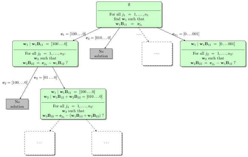
Figure 6: First steps of DERPIA starting from the root of the decoding tree.

The first steps of DeRPIA are illustrated in Figure 6. From the root node, several hypotheses are considered for $\mathbf{w}_{1}$. Only those satisfying (5) are kept at Level 1. The nodes at Level 1 are then expanded with candidates for $\mathbf{w}_{2}$. Figure 7 illustrates the behavior of DeRPIA at Level $n_{\text{v}}+1$. Several hypotheses for $\mathbf{w}_{n_{\text{v}}+1}$ are considered. Only those such that (11) is satisfied are kept to form the final unmixing vectors $\mathbf{w}.$

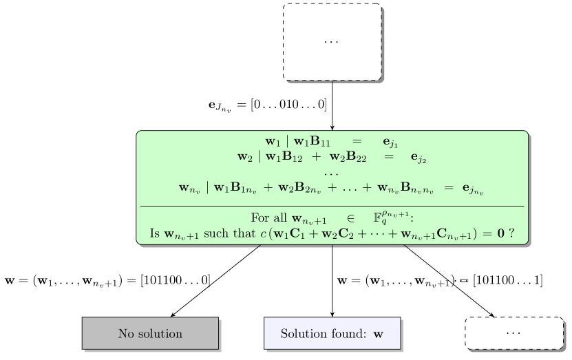
Figure 7: Last steps of DERPIA at the leaves at Level $n_{\text{v}}+1$ of the decoding tree.

IV-B3 Complexity reduction

The aim of this section is to show that at each level of the tree built by DeRPIA, the solution of (13) does not need solving a system of linear equations but may be performed by the search in a look-up table. From Theorem 4, one sees that $\mathbf{w}_{\ell}$ can take at most $\rho_{\ell}+1$ different values, which are the null vector and the canonical base vectors $\mathbf{e}_{i}$ of $\mathbb{F}^{\rho_{\ell}}$ corresponding to the pivots of $\mathbf{B}_{\ell\ell}$.

Theorem 4.

Each $\mathbf{w}_{\ell}$ satisfying (5)-(8) contains at most one non-zero component. In addition, $\mathbf{w}_{1}$ contains exactly one non-zero component.

Proof.

The proof is by contradiction. Consider first $\ell=1$. $\mathbf{B}_{11}$ is a pivot matrix of $\rho{}_{1}$ lines. If $\mathbf{w}_{1}$ contains more than one non-zero component, then $\mathbf{w}_{1}\mathbf{B}_{11}$ will contain more than one non-zero entries corresponding to the pivots of $\mathbf{B}_{11}$ associated to the non-zero components of $\mathbf{w}_{1}$ and (5) cannot be satisfied. Moreover, with $\mathbf{w}_{1}=\mathbf{0}$, (5) cannot be satisfied too.

Consider now some $\ell>1$. In (13), since $\mathbf{TY}$ is in RREF, $\mathbf{B}_{\ell\ell}$ is a pivot matrix of $\rho{}_{\ell}$ lines. Moreover all columns of the matrices $\mathbf{B}_{1,\ell},\dots,\mathbf{B}_{\ell-1,\ell}$ which correspond to the columns of the pivots of $\mathbf{B}_{\ell\ell}$ are zero. This property is shared by the linear combination $\mathbf{w}_{1}\mathbf{B}_{1,\ell}+\dots+\mathbf{w}_{\ell-1}\mathbf{B}_{\ell-1,\ell}$. Thus $\mathbf{e}_{j_{\ell}}-\left(\mathbf{w}_{1}\mathbf{B}_{1,\ell}+\dots+\mathbf{w}_{\ell-1}\mathbf{B}_{\ell-1,\ell}\right)$ is either the null vector, in which case $\mathbf{w}_{\ell}=\mathbf{0}$, or contains at most one non-zero entry due to $\mathbf{e}_{j_{\ell}}$ at the columns corresponding to the pivots of $\mathbf{B}_{\ell\ell}$. In the latter case, if $\mathbf{w}_{\ell}$ contains more than one non-zero component, then $\mathbf{w}_{\ell}\mathbf{B}_{\ell\ell}$ will contain more than one non-zero entry corresponding to the columns of the pivots of $\mathbf{B}_{\ell\ell}$ associated to the non-zero components of $\mathbf{w}_{\ell}$ and (8) cannot be satisfied. ∎

Note that for a given branch, when a set of vectors $\mathbf{w}_{1},\dots,\mathbf{w}_{\ell-1}$ has been found, a vector $\mathbf{w}_{\ell}$ satisfying (5)-(11) does not necessarily exist. In such case the corresponding branch is pruned, see the last case of Example 7 in what follows.

Using Theorem 4, there is no linear system of equations to be solved any more. In practice, the search for $\mathbf{w}_{\ell}$ can be even further simplified using the following corollary.

Corollary 5.

The search for $\mathbf{w}_{\ell}$ satisfying (8) reduces to a simple look-up in a table.

Proof.

Assume that there exists $\mathbf{w}_{\ell}$ satisfying (5)-(11). Then (13) can be rewritten as: $\mathbf{w}_{\ell}\mathbf{B}_{\ell\ell}-\mathbf{e}_{j_{\ell}}=-\left(\mathbf{w}_{1}\mathbf{B}_{1,\ell}+\dots+\mathbf{w}_{\ell-1}\mathbf{B}_{\ell-1,\ell}\right)$. Here we assume that $\mathbf{w}_{\ell}\neq\mathbf{0}$ and then further analyze properties established in Theorem 4:

• In the linear combination $-\left(\mathbf{w}_{1}\mathbf{B}_{1,\ell}+\dots+\mathbf{w}_{\ell-1}\mathbf{B}_{\ell-1,\ell}\right)$, all components that correspond to the columns of the pivots of $\mathbf{B}_{\ell\ell}$ are zero.

• Both sides of (13) can have at most one non-zero entry in the columns of the pivots of $\mathbf{B}_{\ell\ell}$. If there is one, that non-zero entry must correspond to $\mathbf{e}_{j_{\ell}}$.

It follows that $\mathbf{e}_{j_{\ell}}$ must exactly correspond to the component at the column of the unique pivot of $\mathbf{B}_{\ell\ell}$ found in the vector $\mathbf{w}_{\ell}\mathbf{B}_{\ell\ell}$ and must cancel it in the expression $\mathbf{w}_{\ell}\mathbf{B}_{\ell\ell}-\mathbf{e}_{j_{\ell}}$. Since $\mathbf{w}_{\ell}$ (assumed non-zero) has only one non-zero entry and since coefficients corresponding to pivots are equal to $1$, the non-zero component of $\mathbf{w}_{\ell}$ must be $1$ (as it is the case for $\mathbf{e}_{j_{\ell}}$). As a result $\mathbf{w}_{\ell}\mathbf{B}_{\ell\ell}$ is actually one of the row vectors of $\mathbf{B}_{\ell\ell}$, and the expression $\mathbf{w}_{\ell}\mathbf{B}_{\ell\ell}-\mathbf{e}_{j_{\ell}}$ is that row vector with a zero at the place of the component of the associated pivot. Finding one non-zero $\mathbf{w}_{\ell}$ satisfying (5)-(8) is then equivalent to identifying all row vectors $\mathbf{u}$ of $\mathbf{B}_{\ell\ell}$ such that $\overline{\mathbf{u}}=$$-\left(\mathbf{w}_{1}\mathbf{B}_{1,\ell}+\dots+\mathbf{w}_{\ell-1}\mathbf{B}_{\ell-1,\ell}\right)$, where $\overline{\mathbf{u}}=\mathbf{u}-\mathbf{e}_{\gamma\left(\mathbf{u}\right)}$ and $\gamma\left(\mathbf{u}\right)$ is the index of the pivot column of $\mathbf{u}$. ∎

One deduces the following look-up table-based algorithm, which consists in two parts. Algorithm 2a is run once and builds a set of look-up tables from $\mathbf{B}_{1,1},\dots,\mathbf{B}_{n_{\text{v}},n_{\text{v}}}$. Algorithm 2b uses then these look-up tables, takes as input $\left(\mathbf{w}_{1},\dots,\mathbf{w}_{\ell-1}\right)$ satisfying (7) and provides the set of vectors $\left(\mathbf{w}_{1},\dots,\mathbf{w}_{\ell-1},\mathbf{w}_{\ell}\right)$ satisfying (8).

Algorithm 2a. Construction of the look-up tables from $\mathbf{B}_{1,1},\dots,\mathbf{B}_{n_{\text{v}},n_{\text{v}}}$

1. For $\ell=1,\dots,n_{\text{v}}$

   1. Initialization: $\Pi_{\ell}=\emptyset$.

   2. For each row vectors $\mathbf{u}$ of $\mathbf{B}_{\ell\ell}$,

      1. identify the index $\gamma\left(\mathbf{u}\right)$ of its pivot column, and denote by $\overline{\mathbf{u}}$ the row vector with a zero at the place of its pivot: $\overline{\mathbf{u}}=\mathbf{u}-\mathbf{e}_{\gamma\left(\mathbf{u}\right)}$

      2. if $\overline{\mathbf{u}}\notin\Pi_{\ell}$, then $\Pi_{\ell}=\Pi_{\ell}\cup\left\{\overline{\mathbf{u}}\right\}$.

   3. For each $\mathbf{v}\in\Pi_{\ell}$, evaluate

      $$\mathcal{C_{\ell}}\left(\mathbf{v}\right)=\{\mathbf{e}_{i}\in\mathbb{F}_{q}^{\rho_{\ell}},i=1,\dots,\rho_{\ell}|\mathbf{u}\mathrm{\mathbf{\mathbf{=}}\mbox{$\mathbf{e}_{i}$}\mathbf{B}_{\ell\ell}}\mathrm{\leavevmode\nobreak\ and\leavevmode\nobreak\ }\mathbf{u}-\mathbf{e}_{\gamma\left(\mathbf{u}\right)}=\mathbf{v}\}.$$

The sets $\mathcal{C_{\ell}}\left(\mathbf{v}\right)$ contain the candidate $\mathbf{w}_{\ell}$ that may satisfy (8).

Example 6.

Assume for example that

$$\mathbf{B}_{\ell,\ell}=\left(\begin{array}[]{cccccc}1&0&0&0&1&0\\ 0&0&1&0&1&0\\ 0&0&0&1&1&0\\ 0&0&0&0&0&1\end{array}\right).$$

Using Algorithm 2a, one obtains

$$\Pi_{\ell}=\left\{\left(\begin{array}[]{cccccc}0&0&0&0&1&0\end{array}\right),\left(\begin{array}[]{cccccc}0&0&0&0&0&0\end{array}\right)\right\}$$

and

$$\mathcal{C_{\ell}}\left(\left(\begin{array}[]{cccccc}0&0&0&0&1&0\end{array}\right)\right) =\left\{\left(\begin{array}[]{cccc}1&0&0&0\end{array}\right),\left(\begin{array}[]{cccc}0&1&0&0\end{array}\right),\left(\begin{array}[]{cccc}0&0&1&0\end{array}\right)\right\},$$

$$\mathcal{C_{\ell}}\left(\left(\begin{array}[]{cccccc}0&0&0&0&0&0\end{array}\right)\right) =\left\{\left(\begin{array}[]{cccc}0&0&0&1\end{array}\right)\right\}.$$

Algorithm 2b. Obtain the set $\mathcal{W}_{\ell}$ of all $\mathbf{w}_{\ell}$ satisfying (8), from $\left(\mathbf{w}_{1},\dots,\mathbf{w}_{\ell-1}\right)$ satisfying (7).

1. Initialization: $\mathcal{W}_{\ell}=\emptyset$.

2. Compute $\mathbf{v}=-\left(\mathbf{w}_{1}\mathbf{B}_{1,\ell}+\dots+\mathbf{w}_{\ell-1}\mathbf{B}_{\ell-1,\ell}\right)$.

3. If $\mathbf{w}_{\ell}=\mathbf{0}$ satisfies (8), i.e., if $\mathbf{v}+\mathbf{e}_{j_{\ell}}=\mathbf{0}$ for some canonical vector $\mathbf{e}_{j_{\ell}}\in\mathbb{F}_{q}^{L_{\ell}}$, then $\mathcal{W}_{\ell}=\left\{\mathbf{0}\right\}$.

4. If $\mathbf{v}\in\Pi_{\ell}$, then $\mathcal{W}_{\ell}=\mathcal{W}_{\ell}\cup\mathcal{C_{\ell}}(\mathbf{v})$.

Example 7.

Consider the results of Example 6 and a branch at level $\ell-1$ of the decoding tree associated to $\left(\mathbf{w}_{1},\dots,\mathbf{w}_{\ell-1}\right)$. One searches the set of $\mathbf{w}_{\ell}$s satisfying

$$\mathbf{w}_{\ell}\mathbf{B}_{\ell\ell} =\mathbf{e}_{j_{\ell}}-\left(\mathbf{w}_{1}\mathbf{B}_{1,\ell}+\dots+\mathbf{w}_{\ell-1}\mathbf{B}_{\ell-1,\ell}\right).$$ (14)

Assume first that $\left(\mathbf{w}_{1},\dots,\mathbf{w}_{\ell-1}\right)$ is such that

$$\mathbf{v}_{1}\mathbf{=} -\left(\mathbf{w}_{1}\mathbf{B}_{1,\ell}+\dots+\mathbf{w}_{\ell-1}\mathbf{B}_{\ell-1,\ell}\right)$$

$$= \left(\begin{array}[]{cccccc}0&0&0&0&1&0\end{array}\right)$$

then $\mathbf{w=0}$ is a solution of (14) associated to $\mathbf{e}_{j_{\ell}}=\mathbf{e}_{5}=\left(\begin{array}[]{cccccc}0&0&0&0&1&0\end{array}\right)$. The other solutions are given by $\mathcal{C_{\ell}}\left(\mathbf{v}_{1}\right)=\left\{\left(\begin{array}[]{cccc}1&0&0&0\end{array}\right),\left(\begin{array}[]{cccc}0&1&0&0\end{array}\right),\left(\begin{array}[]{cccc}0&0&1&0\end{array}\right)\right\}$ and $\mathcal{W_{\ell}}=\left\{\left(\begin{array}[]{cccc}0&0&0&0\end{array}\right),\left(\begin{array}[]{cccc}1&0&0&0\end{array}\right),\left(\begin{array}[]{cccc}0&1&0&0\end{array}\right),\left(\begin{array}[]{cccc}0&0&1&0\end{array}\right)\right\}$.

Assume now that $\left(\mathbf{w}_{1},\dots,\mathbf{w}_{\ell-1}\right)$ is such that

$$\mathbf{v}_{2}\mathbf{=} -\left(\mathbf{w}_{1}\mathbf{B}_{1,\ell}+\dots+\mathbf{w}_{\ell-1}\mathbf{B}_{\ell-1,\ell}\right)$$

$$= \left(\begin{array}[]{cccccc}0&1&0&0&0&0\end{array}\right),$$

then $\mathbf{w=0}$ is a solution of (14) associated to $\mathbf{e}_{j_{\ell}}=\mathbf{e}_{2}=\left(\begin{array}[]{cccccc}0&1&0&0&0&0\end{array}\right)$. There is no other solution, since $\mathbf{v}_{2}\notin\Pi_{\ell}$.

Assume finally that $\left(\mathbf{w}_{1},\dots,\mathbf{w}_{\ell-1}\right)$ is such that

$$\mathbf{v}_{3}\mathbf{=} -\left(\mathbf{w}_{1}\mathbf{B}_{1,\ell}+\dots+\mathbf{w}_{\ell-1}\mathbf{B}_{\ell-1,\ell}\right)$$

$$= \left(\begin{array}[]{cccccc}1&0&0&1&0&0\end{array}\right),$$

then $\mathcal{W}_{\ell}=\emptyset$, since $\mathbf{w=0}$ is not a solution of (14) and $\mathbf{v}_{3}\notin\Pi_{\ell}$.

V Complexity evaluation

To evaluate the arithmetic complexity of the NeCoRPIA decoding algorithms, one assumes that the complexity of the product of an $n\times m$ matrix and an $m\times p$ matrix is at most $K_{\text{m}}nmp$ operations where $K_{\text{m}}$ is some constant. The complexity of the evaluation of the checksum of a vector in $\mathbb{F}_{q}^{n}$ is $K_{c}n$, where $K_{\text{c}}$ is also a constant. Finally determining whether two vectors of $n$ entries in $\mathbb{F}_{q}$ are equal requires at most $n$ operations.

The decoding complexity of NeCoRPIA depends on several parameters. First, the $g^{\prime}$ received packets of length $L_{\text{x}}$ collected in $\mathbf{Y}^{\prime}$ have to be put in RREF to get $\mathbf{TY}$, introduced in (4). The arithmetic complexity of this operation is $K_{\text{R}}\left(g^{\prime}\right)^{2}L_{\text{x}}$, with $K_{\text{R}}$ a constant.

Algorithm 1 is a tree traversal algorithm. Each branch at Level $\ell$ of the tree corresponds to a partial decoding vector $\left(\mathbf{w}_{1},\dots,\mathbf{w}_{\ell}\right)$ satisfying (5)-(8). The complexity depends on the number of subbranches stemming from this branch and the cost related to the partial verification of (5)-(9) for each of these subbranches. At Level $n_{\text{v}}+1$, for each branch corresponding to a partial decoding vector $\left(\mathbf{w}_{1},\dots,\mathbf{w}_{n_{\text{v}}}\right)$ satisfying (5)-(10), an exhaustive search has to be performed for $\mathbf{w}_{n_{\text{v}}+1}$ such that $\left(\mathbf{w}_{1},\dots,\mathbf{w}_{n_{\text{v}}+1}\right)$ satisfies (5)-(11).

Section V-A evaluates an upper bound for the number of branches at each level of the decoding tree. Section V-B determines the complexity of Algorithm 1 when the satisfying $\mathbf{w}_{\ell}$s are obtained by the solution of a system of linear equations. This version of Algorithm 1 is called DeRPIA-SLE in what follows. Section V-C describes the complexity of Algorithm 1 when the satisfying $\mathbf{w}_{\ell}$s are obtained from look-up tables as described in Algorithms 2a and 2b. This version of Algorithm 1 is called DeRPIA-LUT in what follows. As will be seen, the complexities depend on the ranks $\rho_{1},\dots,\rho_{n_{\text{v}}+1}$, which distribution is evaluated in Section V-E in the case $n_{\text{v}}=1$ and $n_{\text{v}}=2$.

V-A Number of branches in the tree

The following corollary of Theorem 4 provides an evaluation of the number of branches that needs to be explored in Algorithm 1.

Corollary 8.

At Level $\ell$, with $1\leqslant\ell\leqslant n_{\text{v}}$, the maximum number of vectors $\left(\mathbf{w}_{1},\dots,\mathbf{w}_{\ell}\right)$ satisfying (8) is

$$N_{\text{b}}(\ell)=\rho_{1}\left(\rho_{2}+1\right)...\left(\rho_{\ell}+1\right).$$ (15)

The maximum number of branches to be considered by Algorithm 1 at Level $\ell=n_{\text{v}}+1$ is

$$N_{\text{b}}\left(n_{\text{v}}+1\right)=\rho_{1}\left(\rho_{2}+1\right)...\left(\rho_{n_{\text{v}}}+1\right)q^{\rho_{n_{\text{v}}+1}}$$ (16)

and the total number of branches in the decoding tree is upper bounded by

$$N_{\text{b}}=\rho_{1}+\rho_{1}\left(\rho_{2}+1\right)+...+\rho_{1}\left(\rho_{2}+1\right)...\left(\rho_{n_{\text{v}}}+1\right)+\rho_{1}\left(\rho_{2}+1\right)...\left(\rho_{n_{\text{v}}}+1\right)q^{\rho_{n_{\text{v}}+1}}.$$ (17)

Proof.

From Theorem 4, one deduces that $\mathbf{w}_{1}$, of size $\rho_{1}$ can take at most $\rho_{1}$ different values. For $1<\ell\leqslant n_{\text{v}}$, $\mathbf{w}_{\ell}$ of size $\rho_{\ell}$ can either be the null vector or take $\rho_{\ell}$ different non-zero values. For the vector $\mathbf{w}_{n_{\text{v}}+1}$, all possible values $\mathbf{w}_{n_{\text{v}}+1}\in\mathbb{F}_{q}^{\rho_{n_{\text{v}}+1}}$ have to be considered to check whether (11) is verified. The number of vectors $\left(\mathbf{w}_{1},\dots,\mathbf{w}_{\ell}\right)$ satisfying (8) at level $\ell$ is thus upper bounded by the product of the number of possible values of $\mathbf{w}_{k}$, $k=1,\dots,\ell$ which is (15). Similarly, the number of branches that have to be considered at Level $n_{\text{v}}+1$ of the search tree of Algorithm 1 is the product of the number of all possible values of the $\mathbf{w}_{\ell}$, $\ell=1,\dots,n_{\text{v}}+1$ and thus upper-bounded by (16). An upper bound of the total number of branches to consider is then

$$N_{\text{b}}=\sum_{\ell=1}^{n_{\text{v}}+1}N_{\text{b}}(\ell),$$

which is given by (17). ∎

V-B Arithmetic complexity of DeRPIA-SLE

An upper bound of the arithmetic complexity of the tree traversal algorithm, when the number of encoding vectors is $n_{\text{v}}$, is provided by Proposition 9

Proposition 9.

Assume that NeCoRPIA has been performed with $n_{\text{v}}$ random coding subvectors. Then an upper bound of the total arithmetic complexity of DeRPIA-SLE is

$$K_{\text{SLE}}\left(n_{\text{v}}\right) =\sum_{\ell=1}^{n_{\text{v}}+1}N_{\text{b}}\left(\ell-1\right)K\left(\ell\right)$$ (18)

with

$$K\left(1\right) =L_{1}\rho_{1}L_{1},$$

$$K\left(\ell\right) =K_{\text{m}}L_{\ell}\left(\rho_{1}+...+\rho_{\ell-1}\right)+L_{\ell}\left(\ell+\left(\rho_{\ell}+1\right)L_{\ell}\right),$$

$$K\left(n_{\text{v}}+1\right) =K_{\text{m}}gL_{\text{p}}+\left(n_{\text{v}}-1\right)L_{\text{p}}+q^{\rho_{n_{\text{v}}+1}}\left(K_{\text{m}}\rho_{n_{\text{v}}+1}L_{\text{p}}+L_{\text{p}}+K_{\text{c}}L_{\text{p}}\right).$$ (19)

and $N_{\text{b}}\left(0\right)=1$. In the case $n_{\text{v}}=1$, (18) boils down to

$$K_{\text{SLE}}\left(1\right)=\rho_{1}L_{1}^{2}+\rho_{1}L_{\text{p}}\left(K_{\text{m}}g+q^{\rho_{2}}\left(K_{\text{m}}\rho_{2}+1+K_{\text{c}}\right)\right).$$ (20)

The proof of Proposition 9 is given in Appendix -A.

One sees that (18) is expressed in terms of $\rho_{1},\dots,\rho_{n_{\text{v}}+1}$, which are the ranks of the matrices $\mathbf{B}_{\ell\ell}$. As expected, the complexity is exponential in $\rho_{n_{\text{v}}+1}$, which has to be made as small as possible. The values of $\rho_{1},\dots,\rho_{n_{\text{v}}+1}$ depend on those of $L_{\ell}$ and $g$, as will be seen in Section V-E.

V-C Arithmetic complexity of DeRPIA-LUT

The tree obtained with DeRPIA-LUT is the same as that obtained with DeRPIA-SLE. The main difference comes from the arithmetic complexity when expanding one branch of the tree. Algorithm 2a is run only once. Algorithm 2b is run for each branch expansion. An upper bound of the total arithmetic complexity of DeRPIA-LUT is given by the following proposition.

Proposition 10.

Assume that NeCoRPIA has been performed with $n_{\text{v}}$ random coding subvectors. Then an upper bound of the total arithmetic complexity of DeRPIA-LUT is

$$K_{\text{LUT}}\left(n_{\text{v}}\right) =\sum_{\ell=1}^{n_{\text{v}}}\left(K_{\text{LU},\text{1}}\left(\ell\right)+K_{\text{LU},\text{2}}\left(\ell\right)\right)+\sum_{\ell=1}^{n_{\text{v}}}N_{\text{b}}\left(\ell-1\right)K_{\text{LU},3}\left(\ell\right)$$

$$+N_{\text{b}}\left(n_{\text{v}}\right)K\left(n_{\text{v}}+1\right)$$ (21)

with

$$K_{\text{LU},\text{1}}\left(\ell\right) =\rho_{\ell}+L_{\ell}\frac{\rho_{\ell}\left(\rho_{\ell}+1\right)}{2},$$

$$K_{\text{LU},2}\left(\ell\right) =\rho_{\ell}\left(L_{\ell}+1+\rho_{\ell}L_{\ell}\right),$$

$$K_{\text{LU},3}\left(\ell\right) =K_{m}L_{\ell}(\rho_{1}+...+\rho_{\ell-1})+L_{\ell}\left(\ell+\rho_{\ell}\right),$$

and $K\left(n_{\text{v}}+1\right)$ given by (19).

The proof of Proposition 10 is provided in Appendix -B.

Again, as in (18), the complexity (21) depends on the ranks $\rho_{1},\dots,\rho_{n_{\text{v}}+1}$ of the matrices $\mathbf{B}_{\ell\ell}$.

V-D Complexity comparison

When comparing $K_{\text{SLE}}\left(n_{\text{v}}\right)$ and $K_{\text{LUT}}\left(n_{\text{v}}\right)$, one observes that there is a (small) price to be paid for building the look-up tables corresponding to the first sum in (21). Then, the complexity gain provided by the look-up tables appears in the expression of $K_{\text{LU},3}\left(\ell\right)$, which is linear in $L_{\ell}$, whereas $K\left(\ell\right)$ is quadratic in $L_{\ell}$. Nevertheless, the look-up procedure is less useful when there are many terminal branches to consider, i.e., when $\rho_{n_{\text{v}}+1}$ is large, since in this case, the term $N_{\text{b}}\left(n_{\text{v}}\right)K\left(n_{\text{v}}+1\right)$ dominates in both expressions of $K_{\text{SLE}}\left(n_{\text{v}}\right)$ and $K_{\text{LUT}}\left(n_{\text{v}}\right)$.

V-E Distribution of the ranks $\rho_{1},\dots,\rho_{n_{\text{v}}+1}$

Determining the distributions of $\rho_{1},\dots,\rho_{n_{\text{v}}+1}$ in the general case is relatively complex. In what follows, one focuses on the cases $n_{\text{v}}=1$ and $n_{\text{v}}=2$. Experimental results for other values of $n_{\text{v}}$ are provided in Section VI.

V-E1 NC vector with one component, $n_{\text{v}}=1$

In this case, the random NC vectors are gathered in the matrix $\mathbf{V}_{1}$. Once $\mathbf{Y}$ has been put in RREF, the rows of the matrix $\mathbf{B}_{11}$ of rank $\rho_{1}$ are the $\rho_{1}$ linearly independent vectors of $\mathbf{V}_{1}$. The distribution of $\rho_{1}$ may be analyzed considering the classical urn problem described in [39]. This problem may be formulated as: assume that $g$ indistinguishable balls are randomly dropped in $L_{1}$ distinguishable boxes. The distribution of the number $X_{g}^{L_{1}}$ of boxes that contain at least one ball is described in [39] citing De Moivre as

$$P(X_{g}^{L_{1}} =k)=f\left(g,L_{1},k\right),$$ (22)

with

$$f\left(g,L,k\right)=\frac{L(L\text{\textminus}1)\text{$\dots$}(L\text{\textminus}k+1)}{L^{g}}S\left(g,k\right),$$

where $S(g,k)$ denotes the Stirling numbers of the second kind [42]. In the context of NeCorPIA, a collision corresponds to at least two balls dropped in the same box. The probability mass function (pmf) of the rank $\rho_{1}$ of $\mathbf{B}_{11}$ is then that of the number of boxes containing at least one ball and is given by (22). The pmf of $\rho_{2}$ is deduced from (22) as

$$P\left(\rho_{2}=g-k\right) =1-P(\rho_{1}=k)$$

$$=1-f\left(g,L_{1},k\right).$$ (23)

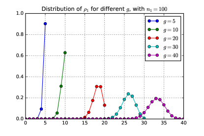
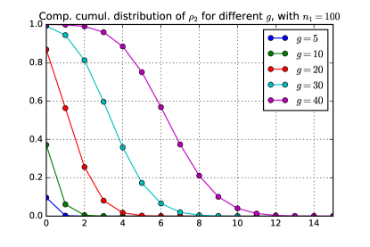
Figure 8: Case $n_{\text{v}}=1$, theoretical and experimental distributions of $\rho_{1}$ (left) and theoretical and practical complementary cumulative distribution function of $\rho_{2}$ (right) for different values of $g$ for $L_{1}=100$.

Figure 8 shows the distribution of $\rho_{1}$ (left) and the complementary cumulative distribution function $\rho_{2}$ (right) for different values of $g$ when $L_{1}=100$. One sees that $\Pr\left(\rho_{2}>1\right)<0.0025$ when $g=5$ and $\Pr\left(\rho_{2}>1\right)<0.062$ when $g=10$. In the decoding complexity, the exponential term of $K\left(n_{\text{v}}+1\right)$ in both (18) and (21) will thus be of limited impact. When $g=30$, $\Pr\left(\rho_{2}>1\right)$ is larger than 94%. The exponential term in the complexity becomes overwhelming in that case.

V-E2 NC vector with two components, $n_{\text{v}}=2$

In this case, the random NC vectors form the matrix $\left(\mathbf{V}_{1},\mathbf{V}_{2}\right)$. The pmf of $\rho_{1}$ is still given by (22). Determining the pmf of the rank $\rho_{2}$ of $\mathbf{B}_{22}$ is much more complicated. Hence, we will first evaluate an upper bound on the probability that $\rho_{3}=0$ and an approximation of the pmf of $\rho_{3}$. Using these results, one will derive an estimate of the pmf of $\rho_{2}$.

In general, to have $\left(\mathbf{V}_{1},\dots,\mathbf{V}_{n_{\text{v}}}\right)$ of full rank, i.e., $\rho_{n_{\text{v}}+1}=0$, it is necessary that no pair of nodes has generated packets with the same random coding subvectors. In the corresponding urn problem, one has now to consider $g$ balls thrown into $L_{1}L_{2}\dots L_{n_{\text{v}}}$ boxes. In the case $n_{\text{v}}=2$, a node selects two random NC subvectors $\mathbf{e}_{i}\in\mathbb{F}_{q}^{L_{1}}$ and $\mathbf{e}_{j}\in\mathbb{F}_{q}^{L_{2}}$. The pair of indices $\left(i,j\right)$ may be interpreted as the row and column index of the box in which a ball has been dropped, when $L_{1}L_{2}$ boxes are arranged in a rectangle with $L_{1}$ rows and $L_{2}$ columns. The probability of having $g$ balls thrown in $L_{1}L_{2}\dots L_{n_{\text{v}}}$ boxes reaching $g$ different boxes, i.e., of having coding subvectors different for all $g$ nodes is $P(X_{g}^{L_{1}\dots L_{n_{\text{v}}}}=g)$ and can again be evaluated with (22).

A rank deficiency happens when the previous necessary condition is not satisfied, but it may also happen in other cases, see Example 3. As a consequence, one only gets the following upper bound

$$P\left(\rho_{1}+\dots+\rho_{n_{\text{v}}}=g\right)\leqslant f\left(g,L_{1}L_{2}\dots L_{n_{\text{v}}},g\right).$$ (24)

If one assumes that the rank deficiency is only due to nodes having selected the same random coding subvectors, similarly, one may apply (22) as in the case $n_{\text{v}}=1$ and get the following approximation

$$P(\rho_{1}+\dots+\rho_{n_{\text{v}}}=k)\approx f\left(g,L_{1}L_{2}\dots L_{n_{\text{v}}},k\right)$$ (25)

which leads to

$$P(\rho_{n_{\text{v}}+1}=g-k)\approx f\left(g,L_{1}L_{2}\dots L_{n_{\text{v}}},k\right).$$ (26)

This is an approximation, since even if all nodes have selected different coding subvectors, we might have a rank deficiency, as illustrated by Example 3.

In the case $n_{\text{v}}=2$, one will now build an approximation of

$$P\left(\rho_{1}=k_{1},\rho_{2}=k_{2},\rho_{3}=k_{3}\right) =P\left(\rho_{2}=k_{2}|\rho_{1}=k_{1},\rho_{3}=k_{3}\right)$$

$$P\left(\rho_{1}=k_{1}|\rho_{3}=k_{3}\right)P\left(\rho_{3}=k_{3}\right).$$ (27)

Using the fact $k_{1}+k_{2}+k_{3}=g$, one has

$$P\left(\rho_{2}=k_{2}|\rho_{1}=k_{1},\rho_{3}=k_{3}\right)=\begin{cases}1&\text{if }k_{2}=g-k_{1}-k_{3}\\ 0&\text{else.}\end{cases}$$

One will assume that the only dependency between $\rho_{1}$, $\rho_{2}$, and $\rho_{3}$ that has to be taken into account is that $\rho_{1}+\rho_{2}+\rho_{3}=g$ and that $P\left(\rho_{3}=k_{3}\right)$ is given by (26). Then (27) becomes

$$P\left(\rho_{1}=k_{1},\rho_{2}=g-k_{1}-k_{3},\rho_{3}=k_{3}\right)= P\left(\rho_{1}=k_{1}\right)f\left(g,L_{1}L_{2},g-k_{3}\right).$$ (28)

Combining (22) and (28), one gets

$$P\left(\rho_{1}=k_{1},\rho_{2}=g-k_{1}-k_{3},\rho_{3}=k_{3}\right)= f\left(g,L_{1},k_{1}\right)f\left(g,L_{1}L_{2},g-k_{3}\right),$$ (29)

which may also be written as

$$P\left(\rho_{1}=k_{1},\rho_{2}=k_{2},\rho_{3}=g-k_{1}-k_{2}\right)= f\left(g,L_{1},k_{1}\right)f\left(g,L_{1}L_{2},k_{1}+k_{2}\right).$$ (30)

Figure 9 (left) shows the joint pmf $P\left(\rho_{1}=k_{1},\rho_{2}=k_{2}\right)$ deduced from (27) as a function of $k_{1}$ and $k_{2}$ for different values of $g$ with $L_{1}=50$ and $L_{2}=50.$ Figure 9 (right) shows the complementary CDF of $\rho_{3}$ again deduced from (27) for different values of $g$ with $L_{1}=50$ and $L_{2}=50.$ Now, when $g=30$, $\Pr\left(\rho_{3}>1\right)$ is about 1.3%. When $g=40$, $\Pr\left(\rho_{3}>1\right)$ is about 3.8%. In both cases, the exponential term of $K\left(n_{\text{v}}+1\right)$ in (18) and (21) will thus be of limited impact. Considering $n_{\text{v}}=2$ allows one to consider much larger generations than with $n_{\text{v}}=1$.

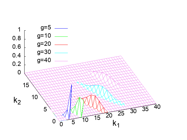
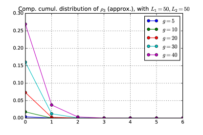
Figure 9: Case $n_{\text{v}}=2$, joint distribution of $\rho_{1}$ and $\rho_{2}$ (left) and approximated complementary cumulative distribution function of $\rho_{3}$ deduced from (26) (right) for different values of $g$ for $L_{1}=50$ and $L_{2}=50$.

Finally, Figure 10 shows the complementary CDF of $\rho_{3}$ for $g=40$ and different values of the pair $\left(L_{1},L_{2}\right)$ such that $L_{1}+L_{2}=100.$ Choosing $L_{1}=L_{2}$ provides the smallest probability of rank deficiency, which is consistent with the hypothesis that the rank deficiency is mainly due to nodes having selected the same random coding subvectors. The maximum of the product $L_{1}\dots L_{n_{\text{v}}}$ with a constraint on $L_{1}+\dots+L_{n_{\text{v}}}$ is obtained taking $L_{1}=L_{2}=\dots=L_{n_{\text{v}}}$.

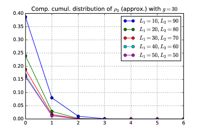
Figure 10: Case $n_{\text{v}}=2$, complementary cumulative distribution function of $\rho_{3}$ deduced from (26) for $g=30$ and different values of $L_{1}$ and $L_{2}$ such that $L_{1}+L_{2}=100$.

VI Performance Evaluation

Several simulation scenarios have been considered to evaluate the performance of NeCorPIA in terms of complexity and decoding error probability. In each simulation run, a set of $g$ packets $\mathbf{x}_{1},\ldots,\mathbf{x}_{g}$ containing $n_{\text{v}}$ random coding subvectors with elements in $\mathbb{F}_{2}$ and with the same STS information are generated. The payload $\mathbf{\boldsymbol{\pi}}=\left(\boldsymbol{\xi},\mathbf{d}\right)$ is replaced by a unique sufficiently long packet identifier to ensure that the $g$ randomly generated packets are linearly independent. Hash functions producing hash of different lengths are considered. In this section, the NC operations are simulated by the generation of a full-rank $g\times g$ random coding matrix $\mathbf{A}$ with elements in $\mathbb{F}_{2}$. The received packets are stored in a matrix $\mathbf{Y=AX}$ of full rank. Writing $\mathbf{Y}$ in RREF, one obtains (4).

In all simulations, the total length $\sum_{\ell=1}^{n_{\text{v}}}L_{\ell}$ of the NC subvectors is fixed at $100$.

Upon completion of Algorithm 1, with the final list of candidate unmixing vectors satisfying (5)-(11), one is always able to get $\mathbf{x}_{1},\ldots,\mathbf{x}_{g}$, since $\mathbf{A}$ is of full rank. Nevertheless, other unmixed packets may be obtained, even if they satisfy all the previous constraints when the rank of the NC header is not sufficient and the hash was inefficient. To evaluate the probability of such event, one considers first the number $n_{\text{w}}$ of different unmixing vectors provided by Algorithm $1$. Among these $n_{\text{w}}$ vectors, $g$ of them lead to the generated packets, the $n_{\text{w}}-g$ others to erroneous packets. Considering a hash of $L_{\text{h}}$ elements of $\mathbb{F}_{q}$, the probability of getting a given hash for a randomly generated payload is uniform and equal to $1/q^{L_{\text{h}}}$. The probability that one of the $n_{\text{w}}-g$ erroneous packets has a satisfying hash is thus $1/q^{L_{\text{h}}}$ and the probability that none of them has a satisfying hash is $\left(1-1/q^{L_{\text{h}}}\right)^{n_{\text{w}}-g}$. The probability of decoding error is then

$$P_{\text{e}}=1-\left(1-1/q^{L_{\text{h}}}\right)^{n_{\text{w}}-g}.$$ (31)

An upper bound for $n_{\text{w}}$ is provided by $N_{\text{b}}\left(n_{\text{v}}+1\right)$. In what follows, this upper bound is used to get an upper bound for $P_{\text{e}}$ evaluated as

$$\overline{P}_{\text{e}}=E\left(1-\left(1-1/q^{L_{\text{h}}}\right)^{N_{\text{b}}\left(n_{\text{v}}+1\right)-g}\right),$$ (32)

where the expectation is taken either considering the pmf of $\left(\rho_{1},\dots,\rho_{n_{\text{V}}+1}\right)$ or an estimated pmf obtained from experiments.

The other metrics used to evaluate the performance of NeCoRPIA are:

• the number of branches explored in the decoding tree before being able to decode all the packets $\mathbf{x}_{1},\ldots,\mathbf{x}_{g}$,

• the arithmetic complexity of the decoding process.

In what follows, to evaluate the complexity, one assumes that $L_{\text{h}}=2$ bytes or $L_{\text{h}}=4$ bytes and that $L_{\text{x}}=256$ bytes. For the various constants in the arithmetic complexity, one chooses $K_{\text{m}}=2$, $K_{\text{R}}=3$, see, e.g., [43], and $K_{\text{c}}=3$, see [44].

Averages are taken over 1000 realizations.

VI-A Case $n_{\text{v}}=1$

The theoretical and experimental distributions of $\rho_{1}$, evaluated using (22), for $L_{1}=100$ and $g=20$, are represented in Figure 8 (left). A very good match between theoretical and experimental distributions is observed.

Figure 11: Case $n_{\text{v}}=1$, theoretical and experimental distributions of $\rho_{1}$ (left) when $g=20$ and theoretical and practical complementary cumulative distribution function of $\rho_{2}$ (right) when $g=20$ for $L_{1}=100$.

For a fixed value of $\rho_{1}$, the upper-bound (16) for the number of branches in the decoding tree boils down to

$$N_{\text{b}}=\rho_{1}+\rho_{1}q^{g-\rho_{1}}.$$

One is then able to evaluate the average value of $N_{\text{b}}$

$$E\left(N_{\text{b}}\right)=\sum_{\rho_{1}=0}^{g}f\left(g,L_{1},\rho_{1}\right)\left(\rho_{1}+\rho_{1}q^{g-\rho_{1}}\right).$$ (33)

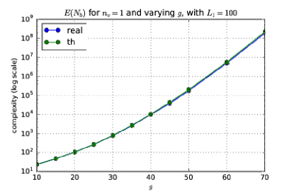
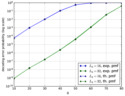
Figure 12: Case $n_{\text{v}}=1$, theoretical and practical values of $E\left(N_{\text{b}}\right)$ (left) of the decoding error probability $\overline{P}_{\text{e}}$ with $L_{\text{h}}=16$ and $L_{\text{h}}=32$ (right) for different values of $g$ when $L_{1}=100$.

Figure 12 represents the theoretical and experimental values of $E\left(N_{\text{b}}\right)$ (left) and of $\overline{P}_{\text{e}}$ (right) as a function of $g$ when $L=100.$ The expression of $E\left(N_{\text{b}}\right)$ provided by (33) as well as that of $\overline{P}_{\text{e}}$ given by (32) match well the experimental results. As expected, for a given value of $g$, the decoding error probability is much less with $L_{\text{\text{h}}}=32$ than with $L_{\text{\text{h}}}=16$. When $g=20$ and $L_{\text{h}}=16$, one gets $\overline{P}_{\text{e}}=10^{-3}$, which may be sufficiently small for some applications.

The arithmetic complexity of both decoding algorithms is then compared to that of a plain NC decoding. The latter requires only a single RREF (once the nodes have agreed on the NC vector they should select). Since both DeRPIA decoding algorithms also require an initial RREF, the complexity ratio is always larger than one.

In the case $n_{\text{v}}=1$, the arithmetic complexity of decoding of plain NC-encoded packets is thus

$$A_{\text{NC}}=3g^{2}L_{\text{x}},$$

where the length $L_{\text{x}}$ is expressed as the number of elements of $\mathbb{F}_{q}$ in which the NC operations are performed. The arithmetic complexities of DeRPIA-SLE and DeRPIA-LUT depend on $\rho_{1}$ and $\rho_{2}$. Their expected values are

$$A_{\text{SLE}}\left(n_{\text{v}}=1\right)\simeq A_{\text{NC}}+E\left[\rho_{1}L_{1}^{2}+\rho_{1}L_{\text{p}}\left(K_{\text{m}}g+q^{\rho_{2}}\left(K_{\text{m}}\rho_{2}+1+K_{\text{c}}\right)\right)\right],$$

and

$$A_{\text{LUT}}\left(n_{\text{v}}=1\right) \simeq A_{\text{NC}}+\sum_{\ell=1}^{2}E\left[\rho_{1}+L_{1}\frac{\rho_{1}\left(\rho_{1}+1\right)}{2}+\rho_{1}\left(L_{1}+1+\rho_{1}L_{1}\right)\right.$$

$$\left.+L_{1}\left(1+\rho_{1}\right)+\rho_{1}L_{\text{p}}\left(K_{\text{m}}g+q^{\rho_{2}}\left(K_{\text{m}}\rho_{2}+1+K_{\text{c}}\right)\right)\right]$$

where the expectation is evaluated using (22) and (23).

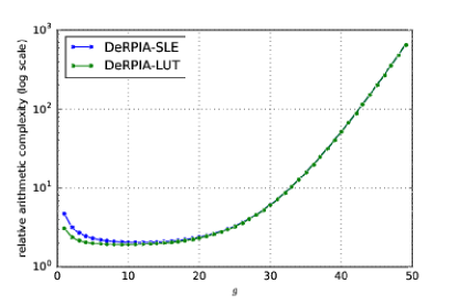
Figure 13: Case $n_{\text{v}}=1$, evolution of the ratio of the expected decoding complexity of DeRPIA-SLE and DeRPIA-LUT with respect to the complexity of a simple RREF transformation for different value of $g$ when $L_{1}=100$.

Figure 13 compares the relative arithmetic complexity of the two variants of DeRPIA with respect to $A_{\text{NC}}$. One sees that $A_{\text{SLE}}$ and $A_{\text{LUT}}$ are about twice that of $A_{\text{NC}}$ when $g\leqslant 25$. When $g\geqslant 30$, the complexity increases exponentially. $A_{\text{LUT}}$ is only slightly less than $A_{\text{SLE}}$ for small values of $g.$ Again, for values of $g$ larger than $25$, the exponential term dominates.

VI-B Case $n_{\text{v}}=2$

In this case, an expression is only available for the pmf of $\rho_{1}$ as a function of $g$ and $L_{1}$, see Section V-E2. Figure 14 represents the histograms of $\rho_{1}$, $\rho_{2}$, and $\rho_{3}$ for different values of $g$, as well as the theoretical pmf of $\rho_{1}$.

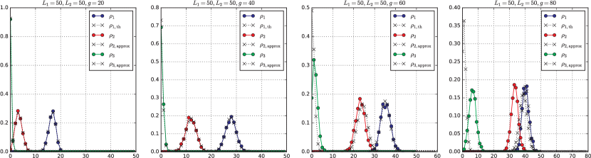
Figure 14: Case $n_{\text{v}}=2$, theoretical pmf of $\rho_{1}$ and histograms of $\rho_{1}$, $\rho_{2}$, and $\rho_{3}$ for different values of $g$ when $L_{1}=L_{2}=50$.

Figure 15 shows that the approximation of $P\left(\rho_{3}=k\right)$ provided by (26) matches well the histogram of $\rho_{3}$ when $g\leqslant 40$. When $g=80$, the approximation is no more valid: the effect of cycles, illustrated in Example 3, becomes significant.

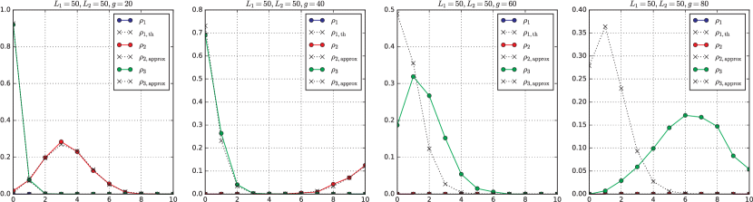
Figure 15: Case $n_{\text{v}}=2$, distribution of $\rho_{1}$ and histograms of $\rho_{1}$, $\rho_{2}$, and $\rho_{3}$ for different values of $g$ for $L_{1}=L_{2}=50$ (zoom of Fig 14).

For the complexity evaluation, in the case $N_{\text{v}}=2$, for a given value of $\rho_{1}$ and $\rho_{2}$, the upper bound (16) becomes

$$N_{\text{b}}=\rho_{1}+\rho_{1}\left(\rho_{2}+1\right)+\rho_{1}\left(\rho_{2}+1\right)q^{g-\rho_{1}-\rho_{2}}.$$ (34)

The average value of $N_{\text{b}}$ is then evaluated using the approximation (30) of the joint pmf of $\left(\rho_{1},\rho_{2},\rho_{3}\right)$ as

$$E\left(N_{\text{b}}\right)=\sum_{\rho_{1}+\rho_{2}\leqslant g}f\left(g,L_{1},\rho_{1}\right)f\left(g,L_{1}L_{2},\rho_{1}+\rho_{2}\right)\left(\rho_{1}+\rho_{1}\left(\rho_{2}+1\right)+\rho_{1}\left(\rho_{2}+1\right)q^{g-\rho_{1}-\rho_{2}}\right).$$ (35)

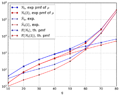
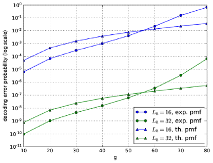
Figure 16: Case $n_{\text{v}}=2$, theoretical and experimental values of $E\left(N_{\text{b}}\left(3\right)\right)$ and $E\left(N_{\text{b}}\right)$ (left) and of the decoding error probability $\overline{P}_{\text{e}}$ with $L_{\text{h}}=16$ and $L_{\text{h}}=32$ (right) for different values of $g$ when $L_{1}=50$ and $L_{2}=50$.

Figure 16 (left) represents the theoretical and experimental values of $E\left(N_{\text{b}}\left(3\right)\right)$ and $E\left(N_{\text{b}}\right)$ as a function of $g$ when $L_{1}=50$ and $L_{2}=50$. The theoretical values of $E\left(N_{\text{b}}\left(3\right)\right)$ and $E\left(N_{\text{b}}\right)$ are evaluated in two ways: First, with the estimated pmf of $\left(\rho_{1},\rho_{2},\rho_{3}\right)$ given by (30) and second with the estimate of this pmf obtained from experiments. The average number $\widetilde{N}_{\text{b}}$ of branches in the tree and in the last level of the tree $\widetilde{N}_{\text{b}}\left(3\right)$ obtained from experiments are also provided. The value of $E\left(N_{\text{b}}\left(3\right)\right)$ and $E\left(N_{\text{b}}\right)$ evaluated from the experimental pmf are good upper-bounds for $\widetilde{N}_{\text{b}}\left(3\right)$ and $\widetilde{N}_{\text{b}}$. The values of $E\left(N_{\text{b}}\left(3\right)\right)$ and $E\left(N_{\text{b}}\right)$ obtained from (30) match well those obtained from the estimated pmf of $\left(\rho_{1},\rho_{2},\rho_{3}\right)$ only for $g\leqslant 50$. When $g\geqslant 60$, the lack of accuracy of the theoretical pmf of $\rho_{3}$ becomes significant: $\widetilde{N}_{\text{b}}\left(3\right)$ and $\widetilde{N}_{\text{b}}$ are underestimated. One observes that considering two encoding subvectors significantly reduces the number of branches that have to be explored in the decoding tree. For example, when $g=70$, $E\left(N_{\text{b}}\right)\simeq 1.6\times 10^{4}$ with $n_{\text{v}}=2$, whereas $E\left(N_{\text{b}}\right)\simeq 1.8\times 10^{8}$ with $n_{\text{v}}=1$.

Figure 16 (right) represents $\overline{P}_{\text{e}}$ obtained from the approximate pmf of $\left(\rho_{1},\rho_{2},\rho_{3}\right)$ given by (30) and from the estimate of this pmf obtained from experiments. Again, both evaluations match well when $g\leqslant 50$. Compared to the case $n_{\text{v}}=1,$ the probability of decoding error reduces significantly thanks to the reduction of the number of branches in the decoding tree at level $n_{\text{v}}+1$.

In the case $n_{\text{v}}=2$, the arithmetic complexity of decoding of plain NC-encoded packets is still $A_{\text{NC}}$. The arithmetic complexities of DeRPIA-SLE and DeRPIA-LUT depend now on $\rho_{1}$, $\rho_{2}$, and $\rho_{3}$. Their expected values are

$$A_{\text{SLE}}\left(n_{\text{v}}=2\right) \simeq A_{\text{NC}}+E\left[\rho_{1}L_{1}^{2}+\rho_{1}L_{2}\left(K_{\text{m}}\rho_{1}+2+\left(\rho_{2}+1\right)L_{2}\right)\right]$$

$$+E\left[\rho_{1}\left(\rho_{2}+1\right)L_{\text{p}}\left(K_{\text{m}}g+1+q^{\rho_{3}}\left(K_{\text{m}}\rho_{3}+1+K_{\text{c}}\right)\right)\right]$$

and

$$A_{\text{LUT}}\left(n_{\text{v}}=2\right) \simeq A_{\text{NC}}+\sum_{\ell=1}^{2}E\left[\rho_{\ell}+L_{\ell}\frac{\rho_{\ell}\left(\rho_{\ell}+1\right)}{2}+\rho_{\ell}\left(L_{\ell}+1+\rho_{\ell}L_{\ell}\right)\right]$$

$$+E\left[L_{1}\left(1+\rho_{1}\right)+\rho_{1}L_{2}\left(K_{m}\rho_{1}+2+\rho_{2}\right)\right]$$

$$+E\left[\rho_{1}\left(\rho_{2}+1\right)L_{\text{p}}\left(K_{\text{m}}g+1+q^{\rho_{3}}\left(K_{\text{m}}\rho_{3}+1+K_{\text{c}}\right)\right)\right]$$

where the expectations are evaluated using (30).

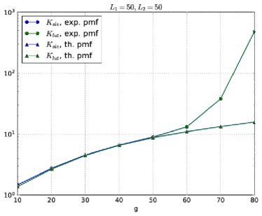
Figure 17: Case $n_{\text{v}}=2$, evolution of the theoretical and experimental values of the ratio of the expected decoding complexity of DeRPIA-SLE and DeRPIA-LUT with respect to the complexity of a simple RREF transformation as a function of $g$ when $L_{1}=L_{2}=50$.

Figure 17 compares the relative arithmetic complexity of the two variants of DeRPIA with respect to $A_{\text{NC}}$. One sees that $A_{\text{SLE}}$ and $A_{\text{LUT}}$ are almost equal and less than ten times $A_{\text{NC}}$ when $g\leqslant 50$. When $g\geqslant 60$, the complexity increases exponentially. This is again not well predicted by the theoretical approximation, due to the degraded accuracy of the theoretical expression of $\rho_{3}$ when $g\geqslant 60$. $A_{\text{LUT}}$ is again only slightly less than $A_{\text{SLE}}$ for small values of $g.$ Now, the exponential term dominates in the complexity for values of $g$ larger than $70$.

VI-C Case $n_{\text{v}}>2$

In this case, since even an approximate expression of the joint pmf of $\left(\rho_{1},\dots,\rho_{n_{\text{v}}+1}\right)$ is difficult to obtain, only the pmf of $\rho_{1}$ and the histograms for $\rho_{2},\dots,\rho_{n_{\text{v}}+1}$ are provided, see Figure (18) for $n_{\text{v}}=3$ and Figure (19) for $n_{\text{v}}=4$.

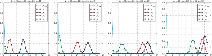
Figure 18: Case $n_{\text{v}}=3$, distribution of $\rho_{1}$ and histograms of $\rho_{1}$, $\rho_{2}$, $\rho_{3}$, and $\rho_{4}$ for different values of $g$ for $L_{1}=33$, $L_{2}=33$, $L_{3}=34$.

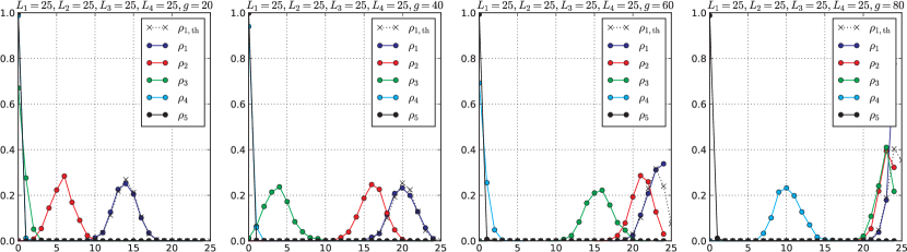
Figure 19: Case $n_{\text{v}}=4$, distribution of $\rho_{1}$ and histograms of $\rho_{1}\dots\rho_{5}$ for different values of $g$ for $L_{1}=\dots=L_{4}=25$.

One observes that when $n_{\text{v}}=4$, even for $g=80$, $P\left(\rho_{5}\geqslant 1\right)\leqslant 0.012$. The contribution of the exponential term in the decoding complexity will thus remain negligible. This can be observed in Figure 20, which shows the evolution of the ratio of the decoding complexity of DeRPIA-SLE and DeRPIA-LUT with respect to the complexity of a simple RREF transformation as a function of $g$ for different values of $n_{\text{v}}$. For values of $g$ for which $\rho_{n_{\text{v}}+1}$ remains small, the complexity increases with $n_{\text{v}}$, due to the increasing number of branches that have to be considered at intermediate levels of the decoding tree. When $\rho_{n_{\text{v}}+1}$ increases, the complexity is dominated by the exponential term in the complexity due to the number of branches to consider at level $n_{\text{v}}+1$ in the decoding tree. Considering a larger value of $n_{\text{v}}$ becomes then interesting from a complexity point of view. This phenomenon appears when $g\geqslant 30$ for $n_{\text{v}}=1$, when $g\geqslant 80$ for $n_{\text{v}}=2$ and does not appear for larger values of $n_{\text{v}}$.

The proposed NeCoRPIA scheme is thus able to perform NC without coordination between agents. With $n_{\text{v}}=2$, compared to classical NC, generations of 60 packets may be considered with a header overhead of 66 %, a vanishing decoding error probability, and a decoding complexity about 10 times that of Gaussian elimination. With $n_{\text{v}}=3$, generations of 80 packets may be considered, leading to a header overhead of 25 %, but a decoding complexity about 100 times that of Gaussian elimination.

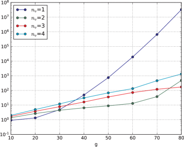
Figure 20: Evolution of the experimental values of the ratio of the decoding complexity of DeRPIA-SLE and DeRPIA-LUT with respect to the complexity of a simple RREF transformation as a function of $g$ for different values of $n_{\text{v}}.$

VII Comparison of packet header overhead

This section aims at comparing the NC header overhead when considering the NC headers of NeCorPIA and a variant of COPE, the variable-length headers proposed in [18].

For that purpose, one considers a simulation framework with $N+1$ nodes randomly spread over a square of unit area. Nodes are able to communicate if they are at a distance of less than $r$. One has adjusted $r$ in such a way that the diameter of the graph associated to the network is $10$ and the minimum connectivity degree is larger than $2$. Without loss of generality, one takes Node $N+1$ is the sink and one selects $g$ randomly chosen nodes among the $N$ remaining nodes are source nodes. During one simulation corresponding to a single STS, each source node generates a single packet. The time in a STS is further slotted and packets are transmitted at the beginning of each time slot. The packet forwarding strategy described in [17] is implemented with constant forwarding factor $d=1.5$, according to Algorithm 4 in [17]. The forwarding factor determines the average number of linear combinations of already received packets a node has to broadcast in the next slot, each time it receives an innovative packet in the current slot. A packet reaching the sink is no more forwarded. The simulation is ended once the sink is able to decode the $g$ source packets of the considered STS. In practice, the source node only controls the duration of a STS and does not know precisely $g$ during the considered STS. This duration may be adapted by the sink to have a prescribed number of active source nodes during an STS. Nevertheless, such algorithm goes beyond the scope of this paper and to simplify, $g$ is assumed to be known.

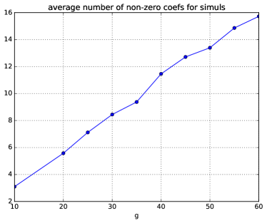
Figure 21: Average number of non-zero coefficients in plain NC headers as a function of $g$

For the COPE-inspired variable-length NC protocol (called COPE in what follows), instead of considering a fixed-length 32-bit packet identifier as in [18], one assumes that the maximum number of active nodes in a STS is known. Then the length of the identifier is adjusted so as to have a probability of collision of two different packets below some specified threshold $p_{\text{c}}$. The packet identifier may be a hash of the packet header and content, as in [18]. Here, to simplify evaluations, it is considered as random, with a uniform distribution over the range of possible identifier values.

For NeCoRPIA, NC headers of $n_{\text{v}}$ blocks of length $L_{1}=\dots=L_{n_{\text{v}}}$ are considered. To limit the decoding complexity, the length of each block is adjusted in such a way that, in average, the estimate of the upper bound of the number of branches in the last level of the decoding tree (16) is less than $10^{3}$. This average is evaluated combining (16) with (23) when $n_{\text{v}}=1$ and (16) with (29) when $n_{\text{v}}=2$. Then, the size of the hash is adjusted in such a way that, in case of collision, the probability of being unable to recover the original packets (32) is less than $p_{\text{c}}$.

For plain NC protocol, assuming that Node $i$ uses $\mathbf{e}_{i}\in\mathbb{F}_{2}^{N}$, $i=1,\dots,N$, as NC header as in [20], there is no collision and the header is of length $N$ elements of $\mathbb{F}_{2}$. A distribution of the number of non-zero entries in the NC headers of transmitted packets is estimated, averaging $10$ network realizations. Figure 21 describes the average amount of non-zero coefficients in packets brodcast by the nodes of the network. One observes that this number increases almost linearly with $g$. The number of transmitted packets at simulation termination does not depend on the way headers are represented. The estimated distribution is used to evaluate the average COPE-inspired NC header length.

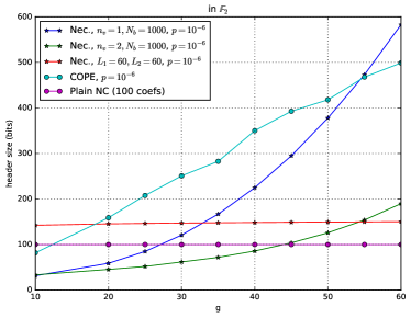
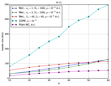
Figure 22: Evolution of the header length as a function of the number of active nodes $g$ in a STS for the plain NC protocol, for COPE, and for NeCoRPIA with $n_{\text{v}}=1$ and $n_{\text{v}}=2$ and subvectors of variable lengths ensuring that the number of decoding hypotheses is less than $N_{b}=1000$, and with $n_{\text{v}}=2$ and fixed subvector lengths $L_{1}=L_{2}=60$; the decoding error probability is imposed to be less than $p_{\text{c}}=10^{-6}$, without entropy coding (left) and with entropy coding of the NC headers (right)

Figure 22 illustrates the evolution of the size of the NC headers as a function of $g$ for plain NC, COPE, and NeCoRPIA headers with $n_{\text{v}}=1$ and $n_{\text{v}}=2$. For the two last approaches, $p_{\text{c}}$ is taken as $10^{-6}$. For NeCoRPIA headers, either a fixed-size header with $L_{1}=L_{2}=60$ is considered or a variable size header that ensures that the number of decoding hypotheses is less than $N_{b}=1000$, limiting thus the decoding complexity. The header overhead necessary to identify the STS is omitted, since it is the same in all cases. In Figure 22 (left), the NC headers are not compressed, wheras in Figure 22 (right), the plain NC and NeCoRPIA headers are assumed to be entropy coded and their coded length is provided.

In absence of entropy coding of the NC header, its size is constant with plain NC. It increases almost linearly with $g$ for COPE and is larger than the header of plain NC as soon as $g\geqslant 12$ and than the NeCoRPIA header in most of the cases. Considering $n_{\text{v}}=2$ and an adaptive header length provides the best results. When $g=40$, the header length of NeCoRPIA is only one fifth of that of COPE. The header length is less than that with plain NC as long as $g<42.$ Thus, without prior agreement of the packets generated in a STS, with NeCoRPIA, one is able to get header length smaller than those obtained with plain NC which requires this agreement phase.

When the NC headers are entropy-coded, the average length of entropy-coded NC headers with plain NC increases almost linearly with $g$. When $n_{\text{v}}=1$, a significant reduction of the header length is obtained by entropy coding, since the header has to be very large to avoid collisions and contains only few non-zero coefficients, see Figure 21. When $n_{\text{v}}=2$, entropy coding reduces slightly the average header length, which remains less than that obtained with $n_{\text{v}}=1$. In average, the compressed header length with NeCoRPIA is only twice that obtained with plain NC.

VIII Conclusions

This paper presents NeCoRPIA, a NC algorithm with random packet index assignment. This technique is well-suited to data collection using MCS, as it does not require any prior agreement on the NC vectors, which are chosen randomly. As a consequence, different packets may share the same coding vector, leading to a collision, and to the impossibility to perform decoding with standard Gaussian elimination. Collisions are more frequent when the size of the generation increases. A branch-and-prune approach is adapted to decode in presence of collisions. This approach is efficient in presence of a low number of collisions. To reduce the number of collisions, we propose to split the NC vector into subvectors. Each packet header consists then of two or more NC subvectors.

A detailed analysis of the decoding complexity and of the probability of decoding error shows the potential of this approach: when a NC of $L=100$ elements in $\mathbb{F}_{2}$ is split into two NC subvectors, generations of about 60 packets may be considered with a decoding complexity that is about $10$ times that of plain network decoding. When the NC vector is split into 4 subvectors, generations of about 80 packets may be considered.

A comparison of the average header length required to get a given probability of network decoding error is provided for a COPE-inspired variable-length NC protocol, for several variants of NeCoRPIA, and for plain NC on random network topologies illustrating the data collection using a network of sensors to a sink. The effect of entropy coding on the header length has also been analyzed. Without and with entropy coding, NeCoRPIA provides header sizes which are significantly smaller than those obtained with COPE. Compared to plain NC, in absence of entropy coding, headers are smaller with NeCoRPIA when the number of active nodes remains moderate.

Future research will be devoted to the development of a data collection protocol based on NeCoRPIA, and more specifically on the adaptation of the STS as a function of the network activity.

-A Arithmetic complexity of DeRPIA-SLE

-A1 Arithmetic complexity for intermediate branches

Consider Level $\ell=1$. For each of the $L_{1}$ canonical vectors $\mathbf{e}_{j_{1}}\in\mathbb{F}_{q}^{L_{1}}$, finding $\mathbf{w}_{1}\in\mathbb{F}_{q}^{\rho_{1}}$ satisfying (13) takes at most $\rho_{1}L_{1}$ operations, since, according to Theorem 4, one searches for a row of $\mathbf{B}_{11}\in\mathbb{F}_{q}^{\rho_{1}\times L_{1}}$ equal to $\mathbf{e}_{j_{1}}$. The arithmetic complexity to get all branches at Level $1$ is thus upper-bounded by

$$K\left(1\right)=L_{1}\rho_{1}L_{1}.$$ (36)

Consider Level $\ell$ with $1<\ell\leqslant n_{\text{v}}$. For each branch associated to a candidate decoding vector $\left(\mathbf{w}_{1},\dots,\mathbf{w}_{\ell-1}\right),$ one first evaluates $-\left(\mathbf{w}_{1}\mathbf{B}_{1,\ell}+\dots+\mathbf{w}_{\ell-1}\mathbf{B}_{\ell-1,\ell}\right)$ which takes $K_{\text{m}}(\rho_{1}L_{\ell}+...+\rho_{\ell-1}L_{\ell})+\left(\ell-1\right)L_{\ell}$ operations, the last term $\left(\ell-1\right)L_{\ell}$ accouting for the additions of the vector-matrix products and the final sign change.

Then, for each of the $L_{\ell}$ canonical vectors $\mathbf{e}_{j_{\ell}}\in\mathbb{F}_{q}^{L_{\ell}}$, evaluating $\mathbf{e}_{j_{\ell}}-\left(\mathbf{w}_{1}\mathbf{B}_{1,\ell}+\dots+\mathbf{w}_{\ell-1}\mathbf{B}_{\ell-1,\ell}\right)$ needs a single addition, and finding $\mathbf{w_{\ell}}$ satisfying (13) takes at most $\rho_{\ell}L_{\ell}$ operations, since one searches for a row of $\mathbf{B}_{\ell\ell}$ equal to $\mathbf{e}_{j_{\ell}}-\left(\mathbf{w}_{1}\mathbf{B}_{1,\ell}+\dots+\mathbf{w}_{\ell-1}\mathbf{B}_{\ell-1,\ell}\right)$. Additionally, one has to verify whether $\mathbf{w_{\ell}}=\mathbf{0}$ is satisfying, which requires $L_{\ell}$ operations.

At Level $\ell$, the arithmetic complexity, for a given candidate $\left(\mathbf{w}_{1},\dots,\mathbf{w}_{\ell-1}\right)$, to find all candidates $\left(\mathbf{w}_{1},\dots,\mathbf{w}_{\ell}\right)$ satisfying (8) is thus upper-bounded by

$$K\left(\ell\right) =K_{\text{m}}\left(\rho_{1}L_{\ell}+...+\rho_{\ell-1}L_{\ell}\right)+\left(\ell-1\right)L_{\ell}+L_{\ell}\left(1+\rho_{\ell}L_{\ell}+L_{\ell}\right)$$ (37)

$$=K_{\text{m}}L_{\ell}\left(\rho_{1}+...+\rho_{\ell-1}\right)+L_{\ell}\left(\ell+\left(\rho_{\ell}+1\right)L_{\ell}\right)$$ (38)

-A2 Arithmetic complexity for terminal branches

Consider now Level $n_{\text{v}}+1$. For each candidate $\left(\mathbf{w}_{1},\dots,\mathbf{w}_{n_{\text{v}}}\right)$, one has first to compute $\mathbf{w}_{1}\mathbf{C}_{1}+...+\mathbf{w}_{n_{\text{v}}}\mathbf{C}_{n_{\text{v}}}$, which requires $K_{\text{m}}\left(\rho_{1}L_{\text{p}}+\rho_{2}L_{\text{p}}+\ldots+\rho_{n_{\text{v}}}L_{\text{p}}\right)+\left(n_{\text{v}}-1\right)L_{\text{p}}\leqslant K_{\text{m}}gL_{\text{p}}+\left(n_{\text{v}}-1\right)L_{\text{p}}$ operations. Then for each candidate $\mathbf{w}_{n_{\text{v}}+1}\in\mathbb{F}_{q}^{\rho_{n_{\text{v}}+1}}$, the evaluation of $\mathbf{w}_{1}\mathbf{C}_{1}+...+\mathbf{w}_{n_{\text{v}}}\mathbf{C}_{n_{\text{v}}}+\mathbf{w}_{n_{\text{v}}+1}\mathbf{C}_{n_{\text{v}}+1}$ and the checksum verification cost $K_{\text{m}}\rho_{n_{\text{v}}+1}L_{\text{p}}+L_{\text{p}}+K_{\text{c}}L_{\text{p}}$ operations. The arithmetic complexity, for a given candidate $\left(\mathbf{w}_{1},\dots,\mathbf{w}_{n_{\text{v}}}\right)$, to find all solutions $\left(\mathbf{w}_{1},\dots,\mathbf{w}_{n_{\text{v}}+1}\right)$ is thus upper-bounded by

$$K\left(n_{\text{v}}+1\right)=K_{\text{m}}gL_{\text{p}}+\left(n_{\text{v}}-1\right)L_{\text{p}}+q^{\rho_{n_{\text{v}}+1}}\left(K_{\text{m}}\rho_{n_{\text{v}}+1}L_{\text{p}}+L_{\text{p}}+K_{\text{c}}L_{\text{p}}\right).$$ (39)

-A3 Total arithmetic complexity of DeRPIA-SLE

To upper bound the arithmetic complexity of the tree traversal algorithm when the number of encoding vectors is $n_{\text{v}}$, one combines (15), (37), and (39) to get (18) with $N_{\text{b}}\left(0\right)=1$. In the case $n_{\text{v}}=1$, (20) follows directly from (18).

-B Arithmetic complexity of DeRPIA-LUT

One first evaluates the complexity of the look-up table construction with Algorithm 2a. The look-up table is built once, after the RREF evaluation. The worst-case complexity is evaluated, assuming that for each row vector $\mathbf{u}$ of $\mathbf{B}_{\ell\ell}$, the resulting vector $\overline{\mathbf{u}}$ is added to $\Pi_{\ell}$.

For each of the $\rho_{\ell}$ lines $\mathbf{u}$ of $\mathbf{B}_{\ell\ell}$, the identification of the index of its pivot column takes at most $L_{\ell}$ operations. The evaluation of $\overline{\mathbf{u}}$ takes one operation. Then determining whether $\overline{\mathbf{u}}\in\Pi_{\ell}$ takes no operation for the first vector ($\Pi_{\ell}$ is empty), at most $L_{\ell}$ operations for the second vector, at most $2L_{\ell}$ operations for the third vector, and at most $\left(\rho_{\ell}-1\right)L_{\ell}$ operations for the last vector. The number of operations required in this step is upper bounded by

$$K_{\text{LU},\text{1}}\left(\ell\right) =\rho_{\ell}\left(L_{\ell}+1\right)+0+L_{\ell}+2L_{\ell}+\dots+\left(\rho_{\ell}-1\right)L_{\ell}$$

$$=\rho_{\ell}+L_{\ell}\frac{\rho_{\ell}\left(\rho_{\ell}+1\right)}{2}.$$ (40)

Then the canonical vectors $\mathbf{e}_{i}\in\mathbb{F}_{q}^{\rho_{\ell}},i=1,\dots,\rho_{\ell}$ have to be partitionned into the various $\mathcal{S_{\ell}}\left(\mathbf{v}\right)$, $\mathbf{v}\in\Pi_{\ell}$. This is done by considering again each of the $\rho_{\ell}$ lines $\mathbf{u}$ of $\mathbf{B}_{\ell\ell}$, evaluating $\mathbf{u}-\mathbf{e}_{\gamma\left(\mathbf{u}\right)}$, which needs up to $L_{\ell}+1$ operations. Then determining the vectors $\mathbf{v}\in\Pi_{\ell}$ such that $\mathbf{u}-\mathbf{e}_{\gamma\left(\mathbf{u}\right)}=\mathbf{v}$ requires at most $\rho_{\ell}L_{\ell}$ operations, since $\Pi_{\ell}$ contains at most $\rho_{\ell}$ vectors of $L_{\ell}$ elements. The number of operations required in this partitionning is upper bounded by

$$K_{\text{LU},2}\left(\ell\right)=\rho_{\ell}\left(L_{\ell}+1+\rho_{\ell}L_{\ell}\right).$$ (41)

Considering a satisfying $\left(\mathbf{w}_{1},\dots,\mathbf{w}_{\ell-1}\right)$ at Level $\ell-1$, the search complexity to find some satisfying $\left(\mathbf{w}_{1},\dots,\mathbf{w}_{\ell-1},\mathbf{w}_{\ell}\right)$ at Level $\ell$ in Algorithm 2b is now evaluated. The evaluation of $\mathbf{v}=-\left(\mathbf{w}_{1}\mathbf{B}_{1,\ell}+\dots+\mathbf{w}_{\ell-1}\mathbf{B}_{\ell-1,\ell}\right)$ takes $K_{\text{m}}(\rho_{1}L_{\ell}+...+\rho_{\ell-1}L_{\ell})+\left(\ell-1\right)L_{\ell}$ operations. Then, determining whether $\mathbf{w}_{\ell}=\mathbf{0}$ satisfies (8), i.e., whether $\mathbf{v}+\mathbf{e}_{j_{\ell}}=\mathbf{0}$ for some canonical vector $\mathbf{e}_{j_{\ell}}\in\mathbb{F}_{q}^{L_{\ell}}$, can be made checking whether $\mathbf{v}$ contains a single non-zero entry in $L_{\ell}$ operations. Finally, the look-up of $\mathbf{v}\in\Pi_{\ell}$ takes at most $\rho_{\ell}L_{\ell}$ operations. In summary, the number of operations required for this part of the algorithm is

$$K_{\text{LU},3}\left(\ell\right) =K_{m}(\rho_{1}L_{\ell}+...+\rho_{\ell-1}L_{\ell})+\left(\ell-1\right)L_{\ell}+L_{\ell}+\rho_{\ell}L_{\ell}$$

$$=K_{m}L_{\ell}(\rho_{1}+...+\rho_{\ell-1})+L_{\ell}\left(\ell+\rho_{\ell}\right).$$ (42)

Compared to the expression of $K\left(\ell\right)$ given by (37), which is quadratic in $L_{\ell}$, $K_{\text{LU},3}\left(\ell\right)$ is linear in $L_{\ell}$.

The complexity of DeRPIA-LUT, given by (21), when the number of encoding vectors is $n_{\text{v}}$, is then obtained combining the results of Corollary 8 with (40), (42), (42), and (39), since Algorithm 2b is not used at Level $n_{\text{v}}+1$.

References

- [1] C. Gomez and J. Paradells, “Urban automation networks: Current and emerging solutions for sensed data collection and actuation in smart cities,” Sensors, vol. 15, no. 9, pp. 22874–22898, 2015.
- [2] B. Guo, Z. Wang, Z. Yu, Y. Wang, N. Y. Yen, R. Huang, and X. Zhou, “Mobile crowd sensing and computing: The review of an emerging human-powered sensing paradigm,” ACM Comput. Surv., vol. 48, pp. 7:1–7:31, 2015.
- [3] A. Al-Fuqaha, M. Guizani, M. Mohammadi, M. Aledhari, and M. Ayyash, “Internet of things: A survey on enabling technologies, protocols, and applications,” IEEE Comm. Surv. Tut., vol. 17, pp. 2347–2376, 2015.
- [4] K. Doppler, M. Rinne, C. Wijting, C. Ribeiro, and K. Hugl, “Device-to-device communication as an underlay to LTE-advanced networks,” IEEE Comm. Mag., vol. 47, no. 12, pp. 42–49, 2009.
- [5] S. Ahmed and S. S. Kanhere, “Hubcode: hub-based forwarding using network coding in delay tolerant networks,” Wireless Comm. and Mob. Comp., vol. 13, no. 9, pp. 828–846, 2013.
- [6] J. Liu, L. Bic, H. Gong, and S. Zhan, “Data collection for mobile crowdsensing in the presence of selfishness,” EURASIP Jnl on Wireless Comm. and Netw., vol. 2016, p. 82, 2016.
- [7] Y. Jung and Y. Baek, “Multi-hop data forwarding method for crowd sensing networks,” Peer-to-Peer Netw. and Appl., vol. 9, no. 4, pp. 628–639, 2016.
- [8] S. Ding, X. He, J. Wang, B. Qiao, and K. Gai, “Static node center opportunistic coverage and hexagonal deployment in hybrid crowd sensing,” Jnl of Signal Proc. Syst., vol. 86, pp. 251–267, 2017.
- [9] C. Jiang, L. Gao, L. Duan, and J. Huang, “Scalable mobile crowdsensing via peer-to-peer data sharing,” IEEE Trans. Mob. Comp., vol. 17, pp. 898–912, 2018.
- [10] J. Weiwei, C. Canfeng, X. Dongliang, and M. Jian, “Efficient data collection in wireless sensor networks by applying network coding,” in Proc. IEEE Int. Conf. Broadband Netw. Multim. Technol., pp. 90–94, Oct 2009.
- [11] L. Keller, E. Atsan, K. J. Argyraki, and C. Fragouli, “Sensecode: Network coding for reliable sensor networks,” TOSN, vol. 9, no. 2, p. 25, 2013.
- [12] R. Prior, D. E. Lucani, Y. Phulpin, M. Nistor, and J. Barros, “Network coding protocols for smart grid communications,” IEEE Trans. Smart Grid, vol. 5, pp. 1523–1531, May 2014.
- [13] A. Paramanathan, S. Thorsteinsson, D. E. Lucani, and F. H. P. Fitzek, “On bridging theory and practice of inter-session network coding for CSMA/CA based wireless multi-hop networks,” Ad Hoc Networks, vol. 24, pp. 148–160, 2015.
- [14] M. Nistor, D. E. Lucani, and J. Barros, “Network coding protocols for data gathering applications,” IEEE Comm. Let., vol. 19, pp. 267–270, 2015.
- [15] M. Kwon and H. Park, “Network coding based evolutionary network formation for dynamic wireless networks,” IEEE Trans. Mob. Comput., pp. 1–1, 2018.
- [16] R. Ahlswede, N. Cai, S.-Y. Li, and R. Yeung, “Network information flow,” IEEE Trans. Inf. Theory, vol. 46, pp. 1204–1216, 2000.
- [17] C. Fragouli, J. Widmer, and J.-Y. Le Boudec, “Efficient broadcasting using network coding,” IEEE/ACM Trans. Netw., vol. 16, pp. 450–463, 2008.
- [18] S. Katti, H. Rahul, W. Hu, D. Katabi, M. Medard, and J. Crowcroft, “Xors in the air: Practical wireless network coding,” IEEE/ACM Trans. Netw., vol. 16, pp. 497 –510, 2008.
- [19] S. Chachulski, M. Jennings, S. Katti, and D. Katabi, “Trading structure for randomness in wireless opportunistic routing,” in Proc. ACM SIGCOMM, (New York, NY, USA), pp. 169–180, 2007.
- [20] P. Chou, Y. Wu, and K. Jain, “Practical network coding,” in Proc. of Allerton Conf. on Commun. Control and Comput., (Monticello, IL, USA), Oct. 2003.
- [21] J. K. Sundararajan, D. Shah, M. Medard, S. Jakubczak, M. Mitzenmacher, and J. Barros, “Network coding meets tcp: Theory and implementation,” Proc. IEEE, vol. 99, pp. 490–512, 2011.
- [22] L. Xie, P. H. Chong, I. W. Ho, and Y. Guan, “A survey of inter-flow network coding in wireless mesh networks with unicast traffic,” Comp. Netw., vol. 91, pp. 738 – 751, 2015.
- [23] H. Seferoglu, A. Markopoulou, and K. K. Ramakrishnan, “I2nc: Intra- and inter-session network coding for unicast flows in wireless networks,” in Proc. IEEE INFOCOM, pp. 1035–1043, 2011.
- [24] M. Jafari, L. Keller, C. Fragouli, and K. Argyraki, “Compressed network coding vectors,” in Proc. IEEE ISIT, (Seoul, Republic of Korea), pp. 109–113, 2009.
- [25] S. Feizi, D. E. Lucani, C. W. Sorensen, A. Makhdoumi, and M. Medard, “Tunable sparse network coding for multicast networks,” in Proc. NetCod, pp. 1–6, 2014.
- [26] N. Thomos and P. Frossard, “Toward one symbol network coding vectors,” IEEE Commun. Lett., vol. 16, no. 11, pp. 1860–1863, 2012.
- [27] D. Gligoroski, K. Kralevska, and H. Øverby, “Minimal header overhead for random linear network coding,” in Proc. IEEE ICC, pp. 680–685, 2015.
- [28] O. Gnawali, R. Fonseca, K. Jamieson, D. Moss, and P. Levis, “Collection Tree Protocol,” in Proc. ACM SenSys, 2009.
- [29] S. Kafaie, Y. Chen, O. A. Dobre, and M. H. Ahmed, “Joint inter-flow network coding and opportunistic routing in multi-hop wireless mesh networks: A comprehensive survey,” IEEE Comm. Surv. Tut., vol. 20, pp. 1014–1035, Secondquarter 2018.
- [30] J. Heide, M. V. Pedersen, F. H. Fitzek, and M. Médard, “On Code Parameters and Coding Vector Representation for Practical RLNC,” in Proc. IEEE ICC, pp. 1–5, 2011.
- [31] S. Li and A. Ramamoorthy, “Improved compression of network coding vectors using erasure decoding and list decoding,” IEEE Comm. Let., vol. 14, pp. 749–751, 2010.
- [32] P. Garrido, D. E. Lucani, and R. Agüero, “Markov chain model for the decoding probability of sparse network coding,” IEEE Trans. Comm., vol. 65, pp. 1675–1685, 2017.
- [33] D. E. Lucani, M. V. Pedersen, D. Ruano, C. W. Sørensen, F. H. P. Fitzek, J. Heide, O. Geil, V. Nguyen, and M. Reisslein, “Fulcrum: Flexible network coding for heterogeneous devices,” IEEE Access, pp. 1–1, 2018.
- [34] P. Comon and C. Jutten, Handbook of Blind Source Separation: Independent Component Analysis and Applications. Academic Press, 1st ed., 2010.
- [35] A. Yeredor, “Independent component analysis over galois fields of prime order,” IEEE Trans. Inf. Theory, vol. 57, pp. 5342–5359, 2011.
- [36] I.-D. Nemoianu, C. Greco, M. Cagnazzo, and B. Pesquet-Popescu, “On a hashing-based enhancement of source separation algorithms over finite fields for network coding applications,” IEEE Trans. Multimedia, vol. 16, no. 7, pp. 2011–2024, 2014.
- [37] C. Greco, M. Kieffer, C. Adjih, and B. Pesquet-Popescu, “PANDA: A protocol-assisted network decoding algorithm,” in Proc. IEEE NetCod, (Aalborg, Denmark), pp. 1–6, 2014.
- [38] C. Greco, M. Kieffer, and C. Adjih, “NeCoRPIA: Network coding with random packet-index assignment for mobile crowdsensing,” in Proc. IEEE ICC, pp. 6338–6344, 2015.
- [39] L. Holst, “On birthday, collectors, occupancy and other classical urn problems,” Int. Stat. Rev., vol. 54, no. 1, pp. 15–27, 1986.
- [40] C. Adjih, E. Baccelli and S. Cho, “Broadcast With Network Coding: DRAGONCAST,” Internet-Draft, Network Coding Research Group (NCWCRG), Informational, July 2013.
- [41] C. Adjih, M. Kieffer, and C. Greco, “Network coding with random packet-index assignment for data collection networks,” tech. rep., arXiv:1812.05717, 2018.
- [42] M. Abramowitz and I. A. Stegun, eds., Handbook of Mathematical Functions with Formulas, Graphs, and Mathematical Tables, ch. Stirling Numbers of the Second Kind, pp. 824–825. New-York: Dover, 1972.
- [43] T. H. Cormen, C. E. Leiserson, R. L. Rivest, and C. Stein, Introduction to algorithms. MIT Press, 2009.
- [44] J. D. Touch, “Performance analysis of md5,” in ACM SIGCOMM Comp. Comm. Rev., vol. 25, pp. 77–86, 1995.