Optimal error estimates for analytic continuation in the upper half-plane

Abstract

Analytic functions in the Hardy class $H^{2}$ over the upper half-plane $\mathbb{H}_{+}$ are uniquely determined by their values on any curve $\Gamma$ lying in the interior or on the boundary of $\mathbb{H}_{+}$. The goal of this paper is to provide a sharp quantitative version of this statement. We answer the following question. Given $f$ of a unit $H^{2}$ norm that is small on $\Gamma$ (say, its $L^{2}$ norm is of order $\epsilon$), how large can $f$ be at a point $z$ away from the curve? When $\Gamma\subset\partial\mathbb{H}_{+}$, we give a sharp upper bound on $|f(z)|$ of the form $\epsilon^{\gamma}$, with an explicit exponent $\gamma=\gamma(z)\in(0,1)$ and explicit maximizer function attaining the upper bound. When $\Gamma\subset\mathbb{H}_{+}$ we give an implicit sharp upper bound in terms of a solution of an integral equation on $\Gamma$. We conjecture and give evidence that this bound also behaves like $\epsilon^{\gamma}$ for some $\gamma=\gamma(z)\in(0,1)$. These results can also be transplanted to other domains conformally equivalent to the upper half-plane.

1 Introduction

Our motivation comes from the effort to understand stability of extrapolation of complex electromagnetic permittivity of materials as a function of frequency [26, 15]. An underlying mathematical problem is about identifying a Herglotz function—a complex analytic function in the upper half-plane $\mathbb{H}_{+}$ that has nonnegative imaginary part, given its values at specific points in the upper half-plane or on its boundary. Such functions, and their variants, are ubiquitous in physics. For example, the complex impedance of an electrical circuit as a function of frequency has a similar property. Yet another example, is the dependence of effective moduli of composites on the moduli of its constituents [4, 30]. These functions appear in areas as diverse as optimal design problems [27, 28], nuclear physics [6, 7] and medical imaging [14]. It is simply impossible to enumerate all of the fields in science and engineering where they occur. Notwithstanding a more than a century of attention, Herglotz functions remain at the forefront of research, e.g. [10, 9, 36].

Let us assume that a Herglotz function has been experimentally measured on a curve $\Gamma$ in $\mathbb{H}_{+}$. The measurements may contain small errors and the actual data may no longer come from any Herglotz function. The goal is to find a Herglotz function consistent with such noisy measurements up to a small error. In this paper we are not interested in any specific reconstruction or extrapolation algorithm, of which there is an overabundance in the literature, but rather in characterizing a worst case scenario, where two Herglotz functions differ little at the data points, but may diverge significantly, the further away from the data source we move. Since Herglotz functions that decay at infinity always lie in a Hardy space $H^{2}$ of the upper half-plane, we will ask how large can a Hardy function, representing the difference between two Herglotz extrapolants of the same data be at a specific point $z$ if we know that it is $L^{2}$-small on a curve $\Gamma$ in the upper half-plane $\mathbb{H}_{+}$.

On the one hand complex analytic functions possess a large degree of rigidity, being uniquely determined by values at any infinite set of points in a compact set. This rigidity implies that even very small measurement errors will produce data mathematically inconsistent with values of an analytic function. On the other hand there is a theorem due to Riesz (see e.g. [33]) that restrictions of analytic functions in a Hardy class $H^{2}$ are dense in $L^{2}$ on any smooth bounded curve. Therefore, any data can be extrapolated as an analytic function with arbitrary degree of agreement. The high accuracy of matching will be attained by an increasingly wild behavior away from the curve [12]. To see why this occurs we can examine Carleman formulas [8, 19] expressing values of the analytic function in the domain in terms of its values on a part of the boundary. These formulas are highly oscillatory and reproduce values of analytic functions using delicate exact cancellation properties such functions enjoy. Small measurement errors destroy these exact cancellations and small errors get exponentially amplified. For curves in the interior Carleman type formulas have been developed in [1], but they exhibit the same error amplification feature since they are also based on the same exact cancellation properties of analytic functions.

Typically analytic continuation problems are regularized by placing additional boundedness constraints on the extrapolant. The resulting competition between “rigidity” and “flexibility” of complex analytic functions place such questions between ill and well-posed problems. Our goal is to obtain a quantitative version of such a statement. We therefore formulate the power law transition principle according to which all so regularized analytic continuation problems must exhibit a power law transition from well to ill-posedness. Specifically, if $f(\zeta)$ is bounded in some norm in the space of analytic functions on a domain $\Omega$, and is also of order $\epsilon$ on a curve $\Gamma\subset\overline{\Omega}$ in some other norm (e.g. in $L^{2}(\Gamma)$ or $L^{\infty}(\Gamma)$), then it can be only as large as $C\epsilon^{\gamma(z)}$ at some other point $z\in\Omega\setminus\Gamma$. Moreover $\gamma(z)\in(0,1)$ decreases from 1 to 0, as the point $z$ moves further and further away from $\Gamma$. This general principle in the form of an upper bound has been recently established in [37]. In fact, upper and lower bounds of this form have long been known in the literature, e.g. [5, 29, 34, 16, 38, 17, 11, 37]. However, exact values of $\gamma(z)$ have only recently been obtained in a few special cases [11, 37] by matching bounds and constructions.

The most common regularizing boundedness constraints in the literature are in the $H^{\infty}(\Omega)$ norm. The power law estimates are then derived from a maximum modulus principle. To take a simple example from [37], the modulus of the function $e^{z\ln\epsilon}f(z)$ does not exceed $\epsilon$ on the boundary of the infinite strip $\Re z\in(0,1)$, provided $|f(z)|\leq 1$ in the strip and $|f(iy)|\leq\epsilon$. The maximum modulus principle (or rather its Phragmén-Lindelöf version) then implies that $|f(z)|\leq\epsilon^{1-\Re z}$. The estimate is optimal, since $f(z)=\epsilon e^{-z\ln\epsilon}$ satisfies the constraints and achieves equality in the maximum modulus principle. We believe that the power law transition principle for analytic continuation holds in a wide variety of contexts irrespective of the choice of norms, domain geometries and sources of data.

In this paper we formulate the problem of optimal analytic continuation error estimates using Hilbert space norms, rather than $H^{\infty}$ norms and use variational methods that establish optimal upper bounds on the extrapolation error. The bounds are formulated in terms of the solution of an integral equation. In this new formulation the power law transition principle is contained in a somewhat implicit form. It can be made explicit in those cases where the underlying integral equation can be solved explicitly, as is done in Section 6, and in the companion paper [22]. There we apply our methodology to the setting of [11], but with $L^{2}$ rather than $L^{\infty}$ norms. We recover their power law exponent, suggesting that the exponents must be robust and not very sensitive to the choice of specific norms in the spaces of analytic functions. This phenomenon could be related to the fact that functions with worst extrapolation error can be analytically continued into much larger domains, as is evident from our integral equation, and hence satisfy the required constraints in all $L^{p}$ or $H^{p}$ norms.

Conformal mappings between domains can be used to “transplant” the exponent estimates from one geometry to a different one. For example, we can transplant the exponent obtained in Section 6 for the half-plane to the half-strip $\Re z>0$, $|\Im z|<1$, considered in [37]. The analytic function $f(z)$ is assumed to be bounded in the half-strip and also of order $\epsilon$ on the interval $[-i,i]$ on the imaginary axis. Then any such function must satisfy $|f(x)|\leq C\epsilon^{\gamma(x)}$, $x>0$, where $\gamma(x)=(2/\pi){\rm arccot}(\sinh(\pi x/2))$. Moreover, the estimate is sharp, since it is attained by the function $W(-i\sinh(\pi z/2))$, where $W(\zeta)$ is given by (2.22). This result follows from the observation that $\zeta=-i\sinh(\pi z/2)$ is a conformal map from the half-strip to the upper half-plane, mapping interval $[-i,i]$ to the interval $[-1,1]$. As Trefethen points out in [37], the half-strip geometry gives a stark example of the discrepancy between mathematical well-posedness (the analytic continuation error does go to 0 as $\epsilon\to 0$) and practical well-posedness: At $x=1$ only a quarter of all digits of precision will remain, while at $x=2$ only 1/20th will remain.

We start our analysis by reformulating the problem as a maximization of a linear functional with quadratic inequality constraints, which is why we use Hilbert space norms in the original problem formulation. We then use convex duality to obtain an upper bound on $f(z)$. The conditions of optimality of the bound lead to an integral equation for the worst case function $u(\zeta)$. We conclude that our upper bound is optimal, since $u(\zeta)$ satisfies all the constraints. We show that the power law transition principle is a consequence of the conjectured exponential decay of the eigenvalues and eigenfunctions of the integral operator (see Theorem 2.4). The eigenvalues of the integral operator are also singular values of the restriction operator [23], whose exact exponential decay rates are well-known in some cases [31, 32]. The integral operator in the upper half-plane possesses a special “displacement structure”, and the exponential decay of its eigenvalues follows from the upper bound in [3]. Our numerical computations (with the help of Leslie Greengard) show that this upper bound matches the rate of exponential decay of eigenvalues extremely well, when $\Gamma$ is the interval $[-1,1]+ih$, $h>0$. In this special case the integral operator is also of finite convolution type and upper and lower bounds on the rate of exponential decay of its eigenvalues follow from results of Widom [39]. Our computations show that these bounds are far from optimal.

The paper is organized as follows. In the next section we state and discuss our main results. In section 3 we attempt some a priori analysis of the integral equation generating the maximizer of the analytic continuation error. This exhibits singular features of the integral equation that defeat standard a priori estimates approaches. In section 4 we show how the power law transition principle arises from putative features of the integral equation, such as exponential decay of its eigenvalues. In section 5 we prove that the maximizer of the analytic continuation error can be obtained from the solution of an integral equation. In section 6 we analyze the case when $\Gamma=[-1,1]$ lies on the boundary of $\mathbb{H}_{+}$. In this case we show that the error maximizer also solves an integral equation, but with a singular, non-compact integral operator. This singular equation is then solved explicitly and the exponent $\gamma(z)$ is computed. Examining the formula for $\gamma(z)$ we find a beautiful geometric interpretation of this exponent.

2 Main Results

Notation: Let us write $A\sim B$ as $\epsilon\to 0$, whenever $\displaystyle\lim_{\epsilon\to 0}A/B=1$. Let us also write $A\lesssim B$, if there exists a constant $c$ such that $A\leq cB$ and likewise the notation $A\gtrsim B$ will be used. If both $A\lesssim B$ and $A\gtrsim B$ are satisfied we will write $A\simeq B$.

Let $\Gamma\subset\mathbb{H}_{+}$ be a compact smooth ($C^{1}$) curve. Let $L^{2}(\Gamma):=L^{2}(\Gamma,|\text{d}\zeta|)$. In this paper all the $L^{2}$ spaces will be spaces of complex valued functions. Consider the Hardy space

$$H^{2}=H^{2}(\mathbb{H}_{+}):=\{f\ \text{is analytic in}\ \mathbb{H}_{+}:\sup_{y>0}\|f(\cdot+iy)\|_{L^{2}(\mathbb{R})}<\infty\}.$$ (2.1)

It is well known [24] that a function $f\in H^{2}$ has $L^{2}$ boundary data and that $\|f\|_{H^{2}}=\|f\|_{L^{2}(\mathbb{R})}$ defines a norm in $H^{2}$.

2.1 Interior

Theorem 2.1 (Interior).

Let $\Gamma\Subset\mathbb{H}_{+}$ be a smooth ($C^{1}$), bounded and simple curve and $z\in\mathbb{H}_{+}\setminus\Gamma$ be the extrapolation point. Let $\epsilon>0$ and $f\in H^{2}$ be such that $\|f\|_{H^{2}}\leq 1$ and $\|f\|_{L^{2}(\Gamma)}\leq\epsilon$, then

$$|f(z)|\leq\frac{3}{2}u_{\epsilon,z}(z)\min\left\{\frac{1}{\|u_{\epsilon,z}\|_{H^{2}}},\frac{\epsilon}{\|u_{\epsilon,z}\|_{L^{2}(\Gamma)}}\right\},$$ (2.2)

where $u_{\epsilon,z}$ solves the integral equation

$$({\mathcal{K}}u)(\zeta)+\epsilon^{2}u(\zeta)=p_{z}(\zeta),\qquad\zeta\in\Gamma,$$ (2.3)

with

$$({\mathcal{K}}u)(\zeta)=\frac{1}{2\pi}\int_{\Gamma}\frac{iu(\tau)}{\zeta-\overline{\tau}}|\text{d}\tau|,\qquad\qquad p_{z}(\zeta)=\frac{i}{\zeta-\overline{z}}$$ (2.4)

The theorem is proved in Section 5.

Remark 2.2.

1. ${\mathcal{K}}$ is a compact, self-adjoint and positive operator on $L^{2}(\Gamma)$ (cf. Section 4). In particular, (2.3) has a unique solution $u_{\epsilon,z}\in L^{2}(\Gamma)$.

2. It is evident that ${\mathcal{K}}u$ and $p_{z}$ are well-defined members of $H^{2}(\mathbb{H}_{+})$. Hence, when $\zeta\not\in\Gamma$ the integral equation (2.3) is interpreted as a definition of $u_{\epsilon,z}(\zeta)$. This explains the meaning of the right-hand side in (2.2).

The bound in (2.2) is asymptotically optimal, as $\epsilon\to 0$ since the function

$$M_{\epsilon,z}(\zeta)=u_{\epsilon,z}(\zeta)\min\left\{\frac{1}{\|u_{\epsilon,z}\|_{H^{2}}},\frac{\epsilon}{\|u_{\epsilon,z}\|_{L^{2}(\Gamma)}}\right\}$$ (2.5)

has $L^{2}(\Gamma)$-norm bounded by $\epsilon$ and $H^{2}$-norm bounded by 1. Even though we only required $f$ to be in $H^{2}(\mathbb{H}_{+})$, the optimal function $M_{\epsilon,z}(\zeta)$ is actually analytic in $\mathbb{C}\setminus\overline{\Gamma}$.

We believe that the two quantities under the minimum in (2.5) have the same asymptotics as $\epsilon\to 0$, and hence, the error maximizer can be written either as $u_{\epsilon,z}/\|u_{\epsilon,z}\|_{H^{2}}$ or as $\epsilon u_{\epsilon,z}/\|u_{\epsilon,z}\|_{L^{2}(\Gamma)}$.

Conjecture 2.3.

Let $u_{\epsilon,z}$ be as in Theorem 2.1, then

$$\|u_{\epsilon,z}\|_{L^{2}(\Gamma)}\simeq\epsilon\|u_{\epsilon,z}\|_{H^{2}}.$$ (2.6)

The difficulty in establishing (2.6) is that in this particular equation the solution $u_{\epsilon,z}$ must achieve a delicate balance after the cancellation in (2.3). We will show (see Section 3) that $\|u_{\epsilon,z}\|_{L^{2}(\Gamma)}=o(\epsilon^{-1})$, while

$$\lim_{\epsilon\to 0}{\mathcal{K}}u_{\epsilon,z}=p_{z}$$

both in $L^{2}(\Gamma)$ and pointwise in $\mathbb{H}_{+}$. Therefore, the second term on the left-hand side in (2.3) is infinitesimal compared to other terms and hence represents a delicate matching of the remainder after cancellation in $p_{z}-{\mathcal{K}}u_{\epsilon,z}=\epsilon^{2}u_{\epsilon,z}=o(\epsilon)$ in $L^{2}(\Gamma)$. We will also see that $M_{\epsilon,z}(z)=o(1)$ and $M_{\epsilon,z}(z)\gg\epsilon$ as $\epsilon\downarrow 0$. This implies that if the power law transition principle holds, i.e.

$$M_{\epsilon,z}(z)\sim\epsilon^{\gamma},\qquad\text{as}\qquad\epsilon\to 0,$$ (2.7)

then $\gamma=\gamma_{\Gamma}(z)\in(0,1)$. In (2.7) we abuse our notation convention for $\sim$ for the sake of aesthetics. The mathematically correct statement would be $\ln M_{\epsilon,z}(z)\sim\gamma_{\Gamma}(z)\ln\epsilon$. The exponent $\gamma_{\Gamma}(z)$ is expected to grow smaller the further away point $z$ moves from $\Gamma$, so that $\gamma_{\Gamma}(z)\to 0$ as $z\to\infty$. The genesis of the exponent $\gamma_{\Gamma}(z)$ in (2.7) from equation (2.3) that itself contains no fractional exponents of $\epsilon$, comes from the conjectured exponential decay of eigenvalues $\lambda_{n}$ of ${\mathcal{K}}$.

The exponential upper bound on $\lambda_{n}$ is a consequence of the displacement rank 1 structure:

$$(M{\mathcal{K}}-{\mathcal{K}}M^{*})u=\frac{i}{2\pi}\int_{\Gamma}u(\tau)|d\tau|=:Ru,$$ (2.8)

where $M:L^{2}(\Gamma)\to L^{2}(\Gamma)$ is the operator of multiplication by $\tau\in\Gamma$: $(Mu)(\tau)=\tau u(\tau)$. The operator $R$ on the right-hand side of (2.8) is a rank-one operator, since its range consists of constant functions. Then, according to [3],

$$\lambda_{n+1}\leq\rho_{1}\lambda_{n},\qquad\rho_{1}=\inf_{r\in{\mathcal{M}}}\frac{\max_{\tau\in\Gamma}|r(\tau)|}{\min_{\tau\in\Gamma}|r(\overline{\tau})|},$$ (2.9)

for all $n\geq 1$, where ${\mathcal{M}}$ is the set of all Möbius transformations

$$r(\tau)=\frac{a\tau+b}{c\tau+d}.$$

It is easy to see that $\rho_{1}<1$ by considering Möbius transformations that map upper half-plane into the unit disk. Then $\Gamma$ will be mapped to a curve inside the unit disk, so that $m=\max_{\tau\in\Gamma}|r(\tau)|<1$. By the symmetry property of Möbius transformations the image of $\overline{\Gamma}$ will be symmetric to the image of $\Gamma$ with respect to the inversion in the unit circle. Thus, $\min_{\tau\in\Gamma}|r(\overline{\tau})|=1/m$, so that $\rho_{1}\leq m^{2}<1$. In particular this implies that all eigenvalues have multiplicity 1.

The implied exponential upper bound $\lambda_{n+1}\leq\rho_{1}^{n}\lambda_{1}$ is not the best that one can derive from the rank-1 displacement structure (2.8). According to a theorem of Beckermann and Townsend [3], $\lambda_{n}\leq Z_{n}(\Gamma,\overline{\Gamma})\lambda_{1},$ where $Z_{n}$ is the $n$th Zolotarev number [40]. When $n$ is large, the Zolotarev numbers decay exponentially $\ln Z_{n}(\Gamma,\overline{\Gamma})\sim-n\ln\rho_{\Gamma}$, where $\rho_{\Gamma}$ is the Riemann invariant, whereby the annulus $\{1<|z|<\rho_{\Gamma}\}$ is conformally equivalent to the Riemann sphere with $\Gamma$ and $\overline{\Gamma}$ removed [20]. Hence,

$$\lambda_{n}\lesssim\rho_{\Gamma}^{-n}.$$ (2.10)

We are ready now to relate the spectral exponential decay rates to the power law (2.7). Let $\{e_{n}\}_{n=1}^{\infty}$ denote the orthonormal eigenbasis of ${\mathcal{K}}$. In this basis equation (2.3) diagonalizes:

$$\lambda_{n}u_{n}+\epsilon^{2}u_{n}=\pi_{n},\qquad u_{n}=(u,e_{n})_{L^{2}(\Gamma)},\quad\pi_{n}=(p_{z},e_{n})_{L^{2}(\Gamma)},$$

and is easily solved

$$u_{n}=\frac{\pi_{n}}{\lambda_{n}+\epsilon^{2}}.$$ (2.11)

We will prove that

$$\sum_{n=1}^{\infty}\frac{|\pi_{n}|^{2}}{\lambda_{n}}<+\infty,\qquad\sum_{n=1}^{\infty}\frac{|\pi_{n}|^{2}}{\lambda^{2}_{n}}=+\infty,$$ (2.12)

indicating that the coefficients $\pi_{n}$ must also decay exponentially fast. The power law principle is then a consequence of the strictly exponential decay of eigenvalues $\lambda_{n}$ and coefficients $\pi_{n}$.

Theorem 2.4.

Let $\{e_{n}\}_{n=1}^{\infty}$ denote the orthonormal eigenbasis of ${\mathcal{K}}$, and let $\pi_{n}=(p_{z},e_{n})_{L^{2}(\Gamma)}$. Assume that

$$\lambda_{n}\sim C_{1}e^{-\alpha n},\quad|\pi_{n}|^{2}\sim C_{2}e^{-\beta n},\qquad 0<\alpha<\beta<2\alpha,$$ (2.13)

so that (2.12) holds. Then estimate (2.6) holds, and $M_{\epsilon,z}$, given by (2.5) has the power law asymptotics

$$M_{\epsilon,z}(z)\simeq\epsilon^{\frac{\beta-\alpha}{\alpha}},$$ (2.14)

with implicit constants independent of $\epsilon$.

The theorem is proved in Section 4.2.

Remark 2.5.

The coefficients $\pi_{n}$ of $p_{z}$ in the eigenbasis of ${\mathcal{K}}$ can be expressed in terms of the eigenfunctions $\{e_{n}\}$ (cf. (4.2)):

$$\pi_{n}=2\pi\lambda_{n}\overline{e_{n}(z)}.$$

Conjecture 2.6.

The eigenvalues $\lambda_{n}$ of ${\mathcal{K}}$ and coefficients $\pi_{n}=2\pi\lambda_{n}\overline{e_{n}(z)}$ have exponential decay asymptotics (2.13). Moreover, we also conjecture that the asymptotic upper bound (2.10) captures the rate of exponential decay of $\lambda_{n}$, i.e. $\alpha=\ln\rho_{\Gamma}$.

There is substantial evidence supporting this conjecture, including the explicit formula for $\gamma(z)$ in the limiting case when $\Gamma\subset\partial\mathbb{H}_{+}$, given in Theorem 2.7 below. Also, if the $L^{2}$ norm of $f\in H^{2}$ were of order $\epsilon$ on a compact subdomain $G\subset\mathbb{H}_{+}$, instead of the curve $\Gamma$, then the conjectured asymptotics of $\lambda_{n}$ would hold, as shown in [32], provided the boundary of $G$ is sufficiently smooth. The curve $\Gamma$ could also be regarded as a limiting case of a domain. However, its boundary would not be smooth and the analysis in [32] would not apply.

The operator $\epsilon^{2}+{\mathcal{K}}$ in the integral equation (2.3) is almost singular when $\epsilon$ is small, since ${\mathcal{K}}$ is compact and has no bounded inverse. It was the idea of Leslie Greengard to solve (2.3) directly numerically using quadruple precision floating point arithmetic available in FORTRAN. He has written the code and shared the FORTRAN libraries for Gauss quadrature, linear systems solver and eigenvalues and eigenvectors routines for Hermitian matrices. For the numerical computations we took $\Gamma=[-1,1]+ih$, and extrapolation points $z+ih$, $z\geq 1$. Quadruple precision allowed us to compute all eigenvalues of ${\mathcal{K}}$ that are larger than $10^{-33}$ and solve the integral equation (2.3) for values of $\epsilon$ as low as $10^{-16}$. For this particular choice of $\Gamma$ the operator ${\mathcal{K}}$ is a finite convolution type operator with kernel $k(t)=\frac{i(2\pi)^{-1}}{t+2ih}$. Asymptotics of eigenvalues of positive self-adjoint finite convolution operators with real-valued kernels (i.e. even real functions $k(t)$) were obtained by Widom in [39]. To apply these results we note that $\widehat{k}(\xi)=e^{-2h\xi}\chi_{(0,+\infty)}(\xi)$, which has exact exponential decay when $\xi\to+\infty$. The operator ${\mathcal{K}}_{0}$ with the even real kernel $k_{0}(t)=2\Re k(t)$ has symbol $\widehat{k}_{0}(\xi)=e^{-2h|\xi|}$ to which Widom’s theory applies. Widom’s formula gives

$$\ln\lambda_{n}({\mathcal{K}}_{0})\sim-Wn,\qquad\text{as}\ n\to\infty,\qquad W=-\pi\frac{K\left(\mathop{\mathrm{sech}}\left(\frac{\pi}{2h}\right)\right)}{K\left(\tanh\left(\frac{\pi}{2h}\right)\right)},$$

where $K(k)$ is the complete elliptic integral of the first kind. We therefore obtain an upper bound

$$\ln\lambda_{n}({\mathcal{K}}_{h})\leq\ln\lambda_{n}({\mathcal{K}}_{0})\sim-Wn.$$ (2.15)

The lower bound can be obtained from the same formula using an inequality

$$\lambda_{n}({\mathcal{K}}_{0})\leq\lambda_{n/2}({\mathcal{K}}_{h})+\lambda_{n/2}(\overline{{\mathcal{K}}_{h}})=2\lambda_{n/2}({\mathcal{K}}_{h}),$$

so that

$$\ln\lambda_{n}({\mathcal{K}}_{h})\geq\ln\tfrac{1}{2}+\ln\lambda_{2n}({\mathcal{K}}_{0})\sim-2Wn.$$ (2.16)

Figure 1(a), where $h=1$ supports the exponential decay conjecture (2.13) and shows that estimates (2.15), (2.16) are not asymptotically sharp. By contrast, Figure 1(a) shows that the Beckermann-Townsend upper bound (2.10) matches the asymptotics of $\lambda_{n}$ very well. The explicit transformation $\Psi$ of the extended complex plane with $[-1,1]\pm ih$ removed onto the annulus $\{v\in\mathbb{C}:\rho_{\Gamma}^{-1/2}<v<\rho_{\Gamma}^{1/2}\}$ has been derived in [2, p. 138] in terms of the elliptic functions and integrals

$$\Psi^{-1}(v)=\frac{h}{\pi}\left(\zeta\left(\left.\frac{\ln v}{2\pi i}\right|\tau\right)-\zeta\left(\left.\displaystyle\frac{1}{2}\right|\tau\right)\frac{\ln v}{\pi i}\right),\qquad\tau=\frac{K(1-m)}{K(m)},$$ (2.17)

where $\zeta(z|\tau)$ is the Weierstrass zeta function with quasi-periods $1$ and $i\tau$. The Riemann invariant $\rho_{\Gamma}=e^{2\pi\tau}$ is computed after finding the unique solution $m\in(0,1)$ of

$$K(m)E(x(m)|m)-E(m)F(x(m)|m)=\frac{\pi}{2h},\quad x(m)=\sqrt{\frac{K(m)-E(m)}{mK(m)}}.$$

(a)

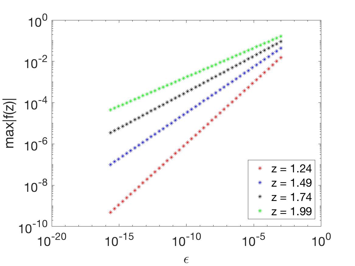
(b)

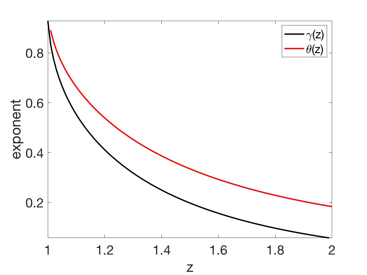
(c)

Figure 1: Numerical support for the power law transition principle.

We can show by a specific construction that one cannot expect better precision at a point $z$ than $\epsilon^{\theta(z)}$ for some $\theta(z)\in(0,1)$, giving an upper bound on $\gamma(z)$. This is done by mapping the explicit eigenfunction expansion of the solution of the integral equation for the annulus problem to the upper half-plane by the explicit conformal transformation $\Psi$ (see [22, 21] for details). This gives the estimate

$$\theta(z)=\frac{\ln|\Psi(\overline{z})|}{\pi\tau}\in(0,1),$$ (2.18)

achieved by the function

$$f(\zeta)=\frac{\epsilon^{2-\theta(z)}}{\zeta+ih}\sum_{n=1}^{\infty}\frac{\left(\overline{\Psi(z)}\Psi(\zeta)\right)^{n}}{\epsilon^{2}+\rho^{-n}}\in H^{2}(\mathbb{H}_{+}).$$ (2.19)

Figure 1(b) shows values of $M_{\epsilon,z}(z)$ as a function of $\epsilon$, supporting the power law principle (2.7). We also compare the computed exponents $\gamma_{\Gamma}(z)$ with the estimate (2.18) for $\Gamma=[-1,1]+0.5i$, and extrapolation points $z+0.5i$, $z>1$. Figure 1(c) shows $\gamma(z)$ (obtained by least squares linear fit of the data for various values of $z$, four of which are shown in Figure 1(b)) and the upper bound $\theta(z)$ given by (2.18). We remark that by virtue of transplanting the actual maximizer of $|f(z)|$ from one geometry to the other, the structure of the test function (2.19) resembles the optimal one (2.11). In fact, for values of $h>0.6$ the bound $\theta(z)$ is virtually indistinguishable from $\gamma_{\Gamma}(z)$.

2.2 Boundary

We recall that functions in the Hardy space $H^{2}$ (see (2.1)) are determined uniquely not only by their values on any curve $\Gamma\subset\mathbb{H}_{+}$, but also on $\Gamma\subset\mathbb{R}$. Indeed, if $f=0$ on $\Gamma\subset\mathbb{R}$, the Cauchy integral representation formula implies

$$f(z)=\frac{1}{2\pi i}\int_{\Gamma^{c}}\frac{f(t)\text{d}t}{t-z},\qquad z\in\mathbb{H}_{+},$$

where $\Gamma^{c}=\mathbb{R}\setminus\Gamma$. Then $f(z)$ has analytic extension to $\mathbb{C}\setminus\Gamma^{c}$, which vanishes on a curve $\Gamma$ inside its domain of analyticity and therefore $f\equiv 0$. This rigidity property suggests that we should expect the same power law behavior of the analytic continuation error as for the curves in the interior of $\mathbb{H}_{+}$.

We will consider the most basic case when $\Gamma\subset\mathbb{R}$ is an interval. (By rescaling and translation we may assume, without loss of generality, that $\Gamma=[-1,1]$). We proceed by representing $\Gamma$ as a limit of interior curves $\Gamma_{h}=[-1,1]+ih$ as $h\downarrow 0$. For curves $\Gamma_{h}$, Theorem 2.1 can be applied and in the resulting upper bound and the integral equation, limits, as $h\downarrow 0$, can be taken. As a result we obtain

Theorem 2.7 (Boundary).

Let $z=z_{r}+iz_{i}\in\mathbb{H}_{+}$ and $\epsilon\in(0,1)$. Assume $f\in H^{2}$ is such that $\|f\|_{H^{2}}\leq 1$ and $\|f\|_{L^{2}(-1,1)}\leq\epsilon$, then

$$|f(z)|\leq\rho\epsilon^{\gamma(z)}$$ (2.20)

where $\rho^{-2}=\frac{z_{i}}{9}\left(\arctan\frac{z_{r}+1}{z_{i}}-\arctan\frac{z_{r}-1}{z_{i}}\right)$ and

$$\gamma(z)=-\frac{1}{\pi}\arg\frac{z+1}{z-1}\in(0,1)$$ (2.21)

is the angular size of $[-1,1]$ as seen from $z$, measured in units of $\pi$ radians. Moreover, the upper bound (2.20) is asymptotically (in $\epsilon$) optimal and the maximizer that attains the bound up to a multiplicative constant independent of $\epsilon$ is

$$W(\zeta)=\epsilon\frac{p(\zeta)}{\|p\|_{L^{2}(-1,1)}}e^{\frac{i}{\pi}\ln\epsilon\ln\frac{1+\zeta}{1-\zeta}},\qquad\qquad\zeta\in\mathbb{H}_{+}$$ (2.22)

where $p(\zeta)=i/(\zeta-\overline{z})$ and $\ln$ denotes the principal branch of logarithm.

The theorem is proved in Section 6.

Remark 2.8.

1. Our explicit formulas show that the problem of predicting the value of a function at $z=z_{0}\in\mathbb{R}\setminus[-1,1]$ is ill-posed in every sense. Indeed, in the optimal bound (2.20) $\rho\to+\infty$ and $\gamma(z)\to 0$ as $z\to z_{0}$.

2. The set of points $z\in\mathbb{H}_{+}$ for which $\gamma(z)$ is the same is an arc of a circle passing through $-1$ and $1$ that lies in the upper half-plane.

3 A priori estimates

Notation: In this section let $\|\cdot\|$ and $(\cdot,\cdot)$ be the norm and the inner product of $L^{2}(\Gamma)$.

In this section we prove several general properties of solutions of the integral equation (2.3). They show that the solution cannot depend analytically on $\epsilon$, as $\epsilon\to 0$.

Lemma 3.1.

Let $u_{\epsilon}$ solve ${\mathcal{K}}u+\epsilon^{2}u=p_{z}$. Then as $\epsilon\downarrow 0$

• $\displaystyle\|u_{\epsilon}\|\to\infty$

• $\dfrac{u_{\epsilon}}{\|u_{\epsilon}\|}\rightharpoonup\>0$ in $L^{2}(\Gamma)$

• $\dfrac{u_{\epsilon}}{\|u_{\epsilon}\|_{H^{2}}}\rightharpoonup\>0$ in $L^{2}(\mathbb{R})$

Proof.

Part (i). Recalling formula (2.11), we have

$$\|u_{\epsilon}\|^{2}=\sum_{n=1}^{\infty}|u_{n}|^{2}=\sum_{n=1}^{\infty}\frac{|\pi_{n}|^{2}}{(\epsilon^{2}+\lambda_{n})^{2}},$$ (3.1)

and applying Lemma Fatou we conclude that

$$\sum_{n=1}^{\infty}\frac{|\pi_{n}|^{2}}{\lambda_{n}^{2}}\leq\mathop{\underline{\lim}}_{\epsilon\to 0}\|u_{\epsilon}\|^{2}.$$

Hence, boundedness along any subsequence of $\|u_{\epsilon}\|$ implies convergence of the series above, which leads to a contradiction, as observed in Lemma 4.1.

Part (ii). Let $v_{\epsilon}=u_{\epsilon}/\|u_{\epsilon}\|$. Extracting a weakly convergent subsequence in $L^{2}(\Gamma)$ and passing to the limit in

$${\mathcal{K}}v_{\epsilon}+\epsilon^{2}v_{\epsilon}=\frac{p_{z}}{\|u_{\epsilon}\|},$$

using Part (i) of the lemma, we obtain the equation for the weak limit $v_{0}$: ${\mathcal{K}}v_{0}=0$. Hence, by Lemma 4.2, $v_{0}=0$. Since every weakly convergent subsequence of $v_{\epsilon}$ has a zero limit, the entire family $v_{\epsilon}$ converges weakly to 0.

Part (iii). Let now $v_{\epsilon}=u_{\epsilon}/\|u_{\epsilon}\|_{H^{2}}$, and let $v_{\epsilon_{k}}\rightharpoonup\>v_{0}$ in $H^{2}(\mathbb{H}_{+})$. Then passing to the limit in (4.7) we obtain

$$v_{0}(\zeta)=\displaystyle\frac{1}{2\pi i}\int_{\mathbb{R}}\frac{v_{0}(x)dx}{x-\zeta}.$$

Observing that $\|u_{\epsilon}\|_{H^{2}}\geq c\|u_{\epsilon}\|\to\infty$, and repeating the argument in the proof of Part (ii) of the lemma, we get ${\mathcal{K}}v_{0}=0$ on $\Gamma$. Hence $v_{0}=0$ on $\Gamma$, and by analyticity, $v_{0}=0$ on $\mathbb{R}$. ∎

Lemma 3.1 has a number of immediate corollaries, especially when combined with formula (4.12) (see Corollary 4.5) and the Cauchy representation formula for $H^{2}$ functions (4.7). Using the Cauchy representation formula (4.7) part (iii) implies that $u_{\epsilon}(\zeta)/\|u_{\epsilon}\|_{H^{2}}\to 0$, as $\epsilon\to 0$ for all $\zeta\in\mathbb{H}_{+}$. In particular, $u_{\epsilon}(z)/\|u_{\epsilon}\|_{H^{2}}\to 0$, as $\epsilon\to 0$. Applying this fact to (4.12) we conclude that $\|u_{\epsilon}\|_{H^{2}}=o(\epsilon^{-2})$ and that

$$\|u_{\epsilon}\|^{2}=o(\|u_{\epsilon}\|_{H^{2}})=o(\epsilon^{-2}),$$ (3.2)

showing that $\|u_{\epsilon}\|=o(\epsilon^{-1})$ and hence $u_{\epsilon}(z)=o(\epsilon^{-2})$. From the integral equation (2.3) we obtain

$$p_{z}-{\mathcal{K}}u_{\epsilon,z}=\epsilon^{2}u_{\epsilon,z}=o(\epsilon)$$ (3.3)

in $L^{2}(\Gamma)$. Returning to the Cauchy representation formula we conclude from (3.2): $\epsilon^{2}u_{\epsilon}(\zeta)\to 0$, as $\epsilon\to 0$ for all $\zeta\in\mathbb{H}_{+}$. Hence, $p_{z}-{\mathcal{K}}u_{\epsilon,z}\to 0$ pointwise in $\mathbb{H}_{+}$.

4 Justification of the power law transition principle

In this section we prove Theorem 2.4 under slightly more general assumptions. It shows how exponential decay of eigenvalues and eigenfunctions gives rise to power law estimates (2.7). Throughout this section $\|\cdot\|$ and $(\cdot,\cdot)$ denote the norm and the inner product of the space $L^{2}(\Gamma)$.

4.1 Spectral representation of $u_{\epsilon,z}(z)$

We begin by rewriting the value $u_{\epsilon,z}(z)$, in terms of $\lambda_{n}$ and coefficients $\pi_{n}$ of $p_{z}$ in the eigenbasis $\{e_{n}\}$.

Lemma 4.1.

Let $u_{\epsilon,z}$ be the solution of (2.3). Then

$$2\pi u_{\epsilon,z}(z)=\sum_{n=1}^{\infty}\frac{|\pi_{n}|^{2}}{\lambda_{n}(\lambda_{n}+\epsilon^{2})}.$$ (4.1)

Proof.

Observe that

$$(u,p_{z})=\int_{\Gamma}u(\tau)\frac{i}{z-\overline{\tau}}|d\tau|=2\pi({\mathcal{K}}u)(z)$$ (4.2)

for any $u\in L^{2}(\Gamma)$, therefore for the solution $u_{\epsilon,z}$ of (2.3) we have

$$2\pi u_{\epsilon,z}(z)=\frac{1}{\epsilon^{2}}(2\pi p_{z}(z)-2\pi({\mathcal{K}}u_{\epsilon,z})(z))=\frac{1}{\epsilon^{2}}\left(\frac{\pi}{\Im z}-(u_{\epsilon,z},p_{z})\right).$$ (4.3)

Since

$$(u_{\epsilon,z},p_{z})=\sum_{n=1}^{\infty}\frac{|\pi_{n}|^{2}}{\lambda_{n}+\epsilon^{2}},$$

it is easy to see that (4.1) is equivalent to

$$\frac{\pi}{\Im z}=\sum_{n=1}^{\infty}\frac{|\pi_{n}|^{2}}{\lambda_{n}}.$$ (4.4)

Formally the series on the right-hand side of (4.4) can be written as

$$\sum_{n=1}^{\infty}\frac{|\pi_{n}|^{2}}{\lambda_{n}}=({\mathcal{K}}^{-1}p_{z},p_{z}).$$

However, it is easy to see that $p_{z}$ is not in the range of ${\mathcal{K}}$. Indeed, for any $u\in L^{2}(\Gamma)$ its image $f(\zeta)=({\mathcal{K}}u)(\zeta)$ has an analytic extension to $\mathbb{C}\setminus\overline{\Gamma}$, while $p_{z}(\zeta)$ has a pole at $\overline{z}\not\in\overline{\Gamma}$. As a consequence

$$\sum_{n=1}^{\infty}\frac{|\pi_{n}|^{2}}{\lambda^{2}_{n}}=+\infty,$$ (4.5)

since otherwise the function

$$v=\sum_{n=1}^{\infty}\frac{\pi_{n}}{\lambda_{n}}e_{n}$$

would belong to $L^{2}(\Gamma)$ and would have the property ${\mathcal{K}}v=p_{z}$.

The key to understanding the operator ${\mathcal{K}}$ is the observation that its range

$${\mathcal{R}}({\mathcal{K}})=\{f:f={\mathcal{K}}u,\ u\in L^{2}(\Gamma)\}$$

consists of functions that have an analytic extension to functions in $H^{2}(\mathbb{H}_{+})$, moreover for any $f\in H^{2}(\mathbb{H}_{+})$ and $u\in L^{2}(\Gamma)$ we have

$$(u,f)=({\mathcal{K}}u,f)_{H^{2}}.$$ (4.6)

Indeed, changing the order of integration we obtain

$$({\mathcal{K}}u,f)_{H^{2}}=\int_{\mathbb{R}}({\mathcal{K}}u)(x)\overline{f(x)}\text{d}x=\int_{\Gamma}u(\tau)\overline{\left(\displaystyle\frac{1}{2\pi i}\int_{\mathbb{R}}\frac{f(x)\text{d}x}{x-\tau}\right)}|\text{d}\tau|=\int_{\Gamma}u(\tau)\overline{f(\tau)}|\text{d}\tau|=(u,f),$$

where we have used the Cauchy representation formula for $H^{2}(\mathbb{H}_{+})$ functions in terms of their boundary values:

$$f(\zeta)=\displaystyle\frac{1}{2\pi i}\int_{\mathbb{R}}\frac{f(x)\text{d}x}{x-\zeta},\quad\zeta\in\mathbb{H}_{+}.$$ (4.7)

An immediate corollary of (4.6) is

Lemma 4.2.

${\mathcal{R}}({\mathcal{K}})$ is dense in $L^{2}(\Gamma)$.

Proof.

Suppose $u\in L^{2}(\Gamma)$ is orthogonal to ${\mathcal{R}}({\mathcal{K}})$. Then for any $v\in L^{2}(\Gamma)$ we have $({\mathcal{K}}v,u)=0$. Choosing $v=u$ we obtain

$$0=(u,{\mathcal{K}}u)=\|{\mathcal{K}}u\|^{2}_{H^{2}},$$

which implies that ${\mathcal{K}}u=0$. This implies that $u=0$ in $L^{2}(\Gamma)$. This conclusion is obtained by observing that for any $v\in L^{2}(\Gamma)$ the image $f(\zeta)=({\mathcal{K}}v)(\zeta)$ has an analytic extension to $\mathbb{C}\setminus\overline{\Gamma}$ and by the Sokhotski-Plemelj formula

$$[\![{\mathcal{K}}v]\!]_{\overline{\Gamma}}(s)=\frac{v(\tau(s))}{\overline{\dot{\tau}(s)}},$$ (4.8)

where $\tau(s)$ is the arc-length parametrization of $\Gamma$. For an oriented curve $C\subset\mathbb{C}$ with parametrization $\tau(s)$ the notation $[\![f]\!]_{C}(s)$ means

$$[\![f]\!]_{C}(s)=\lim_{\zeta\to\tau(s)^{+}}f(\zeta)-\lim_{\zeta\to\tau(s)^{-}}f(\zeta),$$

where $\zeta\to\tau(s)^{+}$ means that the vectors $\dot{\tau}(s)$, $\zeta-\tau(s)$ form a positively oriented pair.

Thus, if ${\mathcal{K}}u=0$ in $L^{2}(\Gamma)$ it follows that the unique analytic extension of ${\mathcal{K}}u$ is a zero function and (4.8) implies $u=0$. ∎

We remark that in the course of the proof of the Lemma we have also shown that ${\mathcal{K}}$ is a positive operator with trivial null-space. We proceed now to the proof of (4.4) by showing that it is a consequence of a more general and elegant result about the operator ${\mathcal{K}}$ (see Lemma 4.3 below).

On a dense subspace ${\mathcal{R}}({\mathcal{K}})\subset L^{2}(\Gamma)$ we define a new inner product

$$(f,g)_{+}=(f,g)_{H^{2}}=({\mathcal{K}}u,v)_{L^{2}(\Gamma)},\qquad f={\mathcal{K}}u,\quad g={\mathcal{K}}v,$$

where formula (4.6) has been used. Suppose that $f_{n}=(f,e_{n})$ and $g_{n}=(g,e_{n})$, then $f_{n}=\lambda_{n}u_{n}$ and $g_{n}=\lambda_{n}v_{n}$, where $u_{n}=(u,e_{n})$ and $v_{n}=(v,e_{n})$. Then

$$(f,g)_{+}=\sum_{n=1}^{\infty}\lambda_{n}u_{n}\overline{v_{n}}=\sum_{n=1}^{\infty}\frac{f_{n}\overline{g_{n}}}{\lambda_{n}}.$$

We now define the Hilbert space $H_{+}$ as the completion of ${\mathcal{R}}({\mathcal{K}})$ with respect to $\|\cdot\|_{+}$. Then

$$H_{+}=\left\{f\in L^{2}(\Gamma):\|f\|_{+}^{2}:=\sum_{n=1}^{\infty}\frac{|f_{n}|^{2}}{\lambda_{n}}<\infty\right\}$$

is a dense subspace in $H_{0}=L^{2}(\Gamma)$. In particular $\|f\|^{2}_{+}\geq\lambda_{1}^{-1}\|f\|^{2}$.

Lemma 4.3.

$H_{+}$ consists of those functions in $L^{2}(\Gamma)$ that have (a necessarily unique) extension to functions in $H^{2}(\mathbb{H}_{+})$. Moreover,

$$(f,g)_{+}=(f,g)_{H^{2}}.$$ (4.9)

Proof.

Formula (4.9) holds for all $\{f,g\}\subset{\mathcal{R}}({\mathcal{K}})$ by definition. Suppose that $f\in H_{+}$. We define

$$\phi_{N}=\sum_{j=1}^{N}f_{n}e_{n}.$$

Obviously, $\phi_{N}\in{\mathcal{R}}({\mathcal{K}})\subset H^{2}$, since each eigenfunction $e_{n}$ is in ${\mathcal{R}}({\mathcal{K}})$. But then by (4.9), $\phi_{N}$ would be a Cauchy sequence in the $H^{2}$ norm and would have a limit $\phi_{\infty}\in H^{2}$. By construction $\phi_{N}\to f$ in $H_{+}$. In particular $\phi_{N}\to f$ in $L^{2}(\Gamma)$, but $\phi_{N}\to\phi_{\infty}$ in $H^{2}$ and therefore in $L^{2}(\Gamma)$. Hence, $f=\phi_{\infty}$ on $\Gamma$ and $f$ has the extension $\phi_{\infty}\in H^{2}$. Thus, if $\{f,g\}\subset H_{+}$ then $f$ and $g$ have extensions to $\mathbb{H}_{+}$ that are in $H^{2}(\mathbb{H}_{+})$. Moreover, if

$$\psi_{N}=\sum_{j=1}^{N}g_{n}e_{n},$$

then we can pass to the limit on both sides of the equality

$$(\phi_{N},\psi_{N})_{+}=(\phi_{N},\psi_{N})_{H^{2}}$$

and obtain (4.9). To finish the proof we only need to show that restrictions to $\Gamma$ of $H^{2}$ functions are in $H_{+}$. According to (4.6)

$$(e_{n},e_{m})_{H^{2}}=\displaystyle\frac{1}{\lambda_{n}}({\mathcal{K}}e_{n},e_{m})_{H^{2}}=\displaystyle\frac{1}{\lambda_{n}}(e_{n},e_{m})=\frac{\delta_{mn}}{\lambda_{n}}.$$

Hence the eigenbasis functions $e_{n}$ also form an orthogonal system in $H_{+}$, but they are no longer orthonormal. We now take $f\in H^{2}$ and repeat the proof of Bessel’s inequality, using the orthogonality of $\{e_{n}\}$:

$$0\leq\|f-\sum_{n=1}^{N}f_{n}e_{n}\|_{H^{2}}^{2}=\|f\|_{H^{2}}^{2}-2\sum_{n=1}^{N}\overline{f_{n}}(f,e_{n})_{H^{2}}+\sum_{n=1}^{N}\frac{|f_{n}|^{2}}{\lambda_{n}}=\|f\|_{H^{2}}^{2}-\sum_{n=1}^{N}\frac{|f_{n}|^{2}}{\lambda_{n}},$$

since, according to (4.6),

$$(f,e_{n})_{H^{2}}=\displaystyle\frac{1}{\lambda_{n}}(f,{\mathcal{K}}e_{n})_{H^{2}}=\frac{f_{n}}{\lambda_{n}}.$$

Thus,

$$\sum_{n=1}^{N}\frac{|f_{n}|^{2}}{\lambda_{n}}\leq\|f\|_{H^{2}}^{2}$$

and hence the series is convergent, proving that the restriction of $f\in H^{2}$ to $\Gamma$ belongs to $H_{+}$. The Lemma is now proved. ∎

Corollary 4.4.

$$\frac{\pi}{\Im z}=\|p_{z}\|_{H^{2}}^{2}=\|p_{z}\|_{+}^{2}=\sum_{n=1}^{\infty}\frac{|\pi_{n}|^{2}}{\lambda_{n}},$$ (4.10)

establishing (4.4) and hence (4.1), which in the new notation of inner product in $H_{+}$ can also be written as

$$2\pi u_{\epsilon,z}(z)=(u_{\epsilon,z},p_{z})_{+}=(u_{\epsilon,z},p_{z})_{H^{2}}.$$ (4.11)

Lemma 4.1 is now proved. ∎

Corollary 4.5.

By Lemma 4.1

$$2\pi u_{\epsilon,z}(z)=\sum_{n=1}^{\infty}\frac{|\pi_{n}|^{2}}{\lambda_{n}(\lambda_{n}+\epsilon^{2})}=\sum_{n=1}^{\infty}\frac{|\pi_{n}|^{2}}{(\lambda_{n}+\epsilon^{2})^{2}}+\epsilon^{2}\sum_{n=1}^{\infty}\frac{|\pi_{n}|^{2}}{\lambda_{n}(\lambda_{n}+\epsilon^{2})^{2}}=\|u_{\epsilon,z}\|^{2}+\epsilon^{2}\|u_{\epsilon,z}\|^{2}_{+},$$

which in view of Lemma 4.3 proves

$$2\pi u_{\epsilon,z}(z)=\|u_{\epsilon,z}\|_{L^{2}(\Gamma)}^{2}+\epsilon^{2}\|u_{\epsilon,z}\|_{H^{2}}^{2}.$$ (4.12)

Remark 4.6.

For all $\{f,g\}\subset H_{+}$ we can formally write

$$(f,g)_{+}=\sum_{n=1}^{\infty}\frac{f_{n}\overline{g_{n}}}{\lambda_{n}}=({\mathcal{K}}^{-1}f,g).$$ (4.13)

If $f={\mathcal{K}}u$ for some $u\in L^{2}(\Gamma)$, the right-hand side of (4.13) is equal to $(u,g)$. Otherwise, $(f,g)_{+}$ will serve as a definition of $({\mathcal{K}}^{-1}f,g)$.

4.2 From exponential decay to power law

In this section we prove Theorem 2.4. We begin by showing that the first part of the theorem holds under substantially weaker assumptions than (2.13). Here we suppress dependence on $\epsilon$ and $z$ from the notation. So that $u_{\epsilon,z}$ is denoted simply by $u$. As before, $\lambda_{n}$ denote the eigenvalues of ${\mathcal{K}}$ and $\pi_{n}=(p_{z},e_{n})$ are coordinates of $p_{z}$ in the eigenbasis of ${\mathcal{K}}$.

Lemma 4.7.

Let $u$ solve (2.3). Assume that in addition to already proved inequality (2.9) there exist $\tilde{\rho},\sigma,\tilde{\sigma}\in(0,1)$, so that

$$\lambda_{n+1}\geq\tilde{\rho}\lambda_{n},\qquad\displaystyle\frac{|\pi_{n+1}|^{2}}{\lambda_{n+1}}\leq\sigma\frac{|\pi_{n}|^{2}}{\lambda_{n}},\qquad\frac{|\pi_{n}|^{2}}{\lambda^{2}_{n}}\leq\tilde{\sigma}\frac{|\pi_{n+1}|^{2}}{\lambda_{n+1}^{2}},\qquad\forall n\ \text{large}$$ (4.14)

Then $\|u\|\simeq\epsilon\|u\|_{H^{2}}$, i.e. Conjecture 2.3 is true.

Proof.

We have

$$\|u\|_{H^{2}}^{2}=\sum_{n=1}^{\infty}\dfrac{|\pi_{n}|^{2}}{\lambda_{n}(\lambda_{n}+\epsilon^{2})^{2}},\qquad\|u\|^{2}=\sum_{n=1}^{\infty}\dfrac{|\pi_{n}|^{2}}{(\lambda_{n}+\epsilon^{2})^{2}}.$$

Define the switchover index $J=J(\epsilon)$

$$\begin{cases}\lambda_{n}\geq\epsilon^{2}&\forall\ 1\leq n\leq J(\epsilon)\\ \lambda_{n}<\epsilon^{2}&\forall\ n>J(\epsilon)\end{cases}$$ (4.15)

then we see

$$\|u\|_{H^{2}}^{2}\simeq\sum_{n=1}^{J}\frac{|\pi_{n}|^{2}}{\lambda_{n}^{3}}+\frac{1}{\epsilon^{4}}\sum_{n=J+1}^{\infty}\frac{|\pi_{n}|^{2}}{\lambda_{n}},\qquad\|u\|^{2}\simeq\sum_{n=1}^{J}\frac{|\pi_{n}|^{2}}{\lambda_{n}^{2}}+\frac{1}{\epsilon^{4}}\sum_{n=J+1}^{\infty}|\pi_{n}|^{2}.$$ (4.16)

Indeed, for $n\leq J$

$$\frac{1}{4}\dfrac{|\pi_{n}|^{2}}{\lambda_{n}^{3}}\leq\dfrac{|\pi_{n}|^{2}}{\lambda_{n}(\lambda_{n}+\epsilon^{2})^{2}}\leq\dfrac{|\pi_{n}|^{2}}{\lambda^{3}_{n}}$$

while for all $n>J$

$$\frac{1}{4}\dfrac{|\pi_{n}|^{2}}{\lambda_{n}\epsilon^{4}}\leq\dfrac{|\pi_{n}|^{2}}{\lambda_{n}(\lambda_{n}+\epsilon^{2})^{2}}\leq\dfrac{|\pi_{n}|^{2}}{\lambda_{n}\epsilon^{4}}$$

recall that the eigenvalues are labeled in decreasing order: $\lambda_{1}\geq\lambda_{2}\geq...$. Now, the second inequality of (4.14) implies

$$\frac{|\pi_{n}|^{2}}{\lambda_{n}}\leq\sigma^{n-J-1}\frac{|\pi_{J+1}|^{2}}{\lambda_{J+1}},\qquad n\geq J+1\quad\Longrightarrow\quad\sum_{n=J+1}^{\infty}\frac{|\pi_{n}|^{2}}{\lambda_{n}}\leq\frac{1}{1-\sigma}\frac{|\pi_{J+1}|^{2}}{\lambda_{J+1}}$$ (4.17)

But then we can estimate

$$\|u\|_{H^{2}}^{2}\lesssim\frac{1}{\lambda_{J+1}}\left(\sum_{n=1}^{J}\frac{\lambda_{J+1}}{\lambda_{n}^{3}}|\pi_{n}|^{2}+\frac{|\pi_{J+1}|^{2}}{\epsilon^{4}}\right)\lesssim\frac{1}{\lambda_{J+1}}\left(\sum_{n=1}^{J}\frac{|\pi_{n}|^{2}}{\lambda_{n}^{2}}+\frac{|\pi_{J+1}|^{2}}{\epsilon^{4}}\right)\lesssim\frac{\|u\|^{2}}{\epsilon^{2}},$$

where in the last inequality we used the first inequality of (4.14).

In order to prove the reverse inequality we appeal to the third inequality of (4.14), which implies

$$\sum_{n=1}^{J}\frac{|\pi_{n}|^{2}}{\lambda_{n}^{2}}\lesssim\frac{|\pi_{J}|^{2}}{\lambda_{J}^{2}}\leq\lambda_{J}\sum_{n=1}^{J}\frac{|\pi_{n}|^{2}}{\lambda_{n}^{3}}$$ (4.18)

But then we can estimate

$$\epsilon^{2}\|u\|_{H^{2}}^{2}\gtrsim\frac{\epsilon^{2}}{\lambda_{J}}\left(\sum_{n=1}^{J}\frac{|\pi_{n}|^{2}}{\lambda_{n}^{2}}+\frac{1}{\epsilon^{4}}\sum_{n=J+1}^{\infty}|\pi_{n}|^{2}\right)\gtrsim\|u\|^{2},$$

where we also used the first inequality of (4.14): $\lambda_{J}\lesssim\lambda_{J+1}<\epsilon^{2}$ which concludes the proof of the lemma. ∎

Let us now prove the second part of Theorem 2.4, that requires strict exponential asymptotics (2.13), which implies (4.14), and therefore (2.6). In this case formulas (2.2), (4.12) and (3.1) imply

$$M_{\epsilon,z}\simeq\epsilon^{2}\|u\|_{H^{2}}\simeq\epsilon\|u\|=\epsilon\sqrt{\sum_{n=1}^{\infty}\frac{|\pi_{n}|^{2}}{(\epsilon^{2}+\lambda_{n})^{2}}}.$$

Then the conclusion of the second part of Theorem 2.4 follows from the following lemma.

Lemma 4.8.

Let $\{a_{n},b_{n}\}_{n=1}^{\infty}$ be nonnegative numbers such that $a_{n}\simeq e^{-\alpha n}$ and $b_{n}\simeq e^{-\beta n}$ with $0<\beta<\alpha$, where the implicit constants don’t depend on $n$. Let $\delta>0$ be a small parameter, then

$$\sum_{n=1}^{\infty}\frac{b_{n}}{(a_{n}+\delta)^{2}}\simeq\delta^{\frac{\beta}{\alpha}-2}$$ (4.19)

where the implicit constants don’t depend on $\delta$.

Proof.

As in the proof of Lemma 4.7 we introduce the switchover index $J=J(\delta)\in\mathbb{N}$ defined by

$$\begin{cases}a_{n}\geq\delta&\quad\forall\ 1\leq n\leq J\\ a_{n}<\delta&\quad\forall\ n>J\end{cases}$$

Below all the implicit constants in relations involving $\simeq$ or $\lesssim$ will be independent on $\delta$. It is clear that

$$\sum_{n=1}^{\infty}\frac{b_{n}}{(a_{n}+\delta)^{2}}\simeq\sum_{n\leq J}\frac{b_{n}}{a_{n}^{2}}+\frac{1}{\delta^{2}}\sum_{n>J}b_{n}.$$

Note that

$$\sum_{n>J}b_{n}\lesssim\sum_{n>J}e^{-\beta n}\lesssim e^{-\beta(J+1)}.$$

On the one hand, using our assumption on $b_{n}$ we find

$$\sum_{n>J}b_{n}\simeq b_{J+1}\simeq b_{J}.$$ (4.20)

On the other hand

$$\sum_{n\leq J}\frac{b_{n}}{a_{n}^{2}}\lesssim\sum_{n\leq J}e^{(2\alpha-\beta)n}=e^{2\alpha-\beta}\frac{e^{(2\alpha-\beta)J}-1}{e^{2\alpha-\beta}-1}\lesssim e^{(2\alpha-\beta)J}\simeq\frac{b_{J}}{a_{J}^{2}},$$

Thus we conclude

$$\sum_{n\leq J}\frac{b_{n}}{a_{n}^{2}}\simeq\frac{b_{J}}{a_{J}^{2}}.$$ (4.21)

Now $\delta\simeq a_{J}$ and $a_{J}\simeq e^{-\alpha J}$, therefore $e^{-J}\simeq\delta^{\frac{1}{\alpha}}$. Using these along with (4.20) and (4.21) we obtain

$$\sum_{n=1}^{\infty}\frac{b_{n}}{(a_{n}+\delta)^{2}}\simeq\frac{b_{J}}{a_{J}^{2}}+\frac{b_{J}}{\delta^{2}}\simeq\frac{b_{J}}{a_{J}^{2}}\simeq e^{(2\alpha-\beta)J}\simeq\delta^{\frac{\beta}{\alpha}-2}.$$

∎

5 Maximizing the extrapolation error

Notation: In this section it will be convenient to switch notation and let $\|\cdot\|$ and $(\cdot,\cdot)$ be the norm and the inner product of $H^{2}$.

Our goal is to understand how large $|f(z)|$ can be, under the assumptions $\|f\|_{H^{2}}\leq 1$ and $\|f\|^{2}_{L^{2}(\Gamma)}\leq\epsilon$. From the representation formula (4.7) we find

$$f(z)=\frac{1}{2\pi}(f,p),\qquad\qquad p(x)=\frac{i}{x-\overline{z}}$$

on the other hand

$$\|f\|_{L^{2}(\Gamma)}^{2}=({\mathcal{K}}f,f)$$

where

$$({\mathcal{K}}f)(s)=\int_{\mathbb{R}}k(t,s)f(t)\text{d}t,\qquad k(t,s)=\frac{1}{4\pi^{2}}\int_{\Gamma}\frac{|\text{d}\tau|}{(t-\tau)(s-\overline{\tau})},\qquad s\in\mathbb{R},$$

and we see that ${\mathcal{K}}$ is a bounded, positive definite, self-adjoint operator in $H^{2}$. We can interchange the order of integration in the definition of ${\mathcal{K}}f$, use (4.7), and obtain an alternative representation:

$$({\mathcal{K}}f)(s)=\frac{i}{2\pi}\int_{\Gamma}\frac{f(\tau)|\text{d}\tau|}{s-\overline{\tau}},\quad s\in\mathbb{R},\quad f\in H^{2}(\mathbb{H}_{+}).$$ (5.1)

From this representation it is obvious that ${\mathcal{K}}f$ has an analytic extension from $\mathbb{R}$ to $\mathbb{C}\setminus\overline{\Gamma}$ and that its restriction to $\mathbb{H}_{+}$ is of Hardy class $H^{2}$.

Thus we arrive at a convex maximization problem with two quadratic constraints. Since the constraints are invariant with respect to the choice of the constant phase factor for the function $f$, instead of maximizing $|f(z)|$ we consider the equivalent problem of maximizing a real linear functional $\Re(f,p)$:

$$\begin{cases}\tfrac{1}{2\pi}\Re(f,p)\rightarrow\max\\ (f,f)\leq 1\\ \displaystyle({\mathcal{K}}f,f)\leq\epsilon^{2}\end{cases}$$ (5.2)

For every $f$, satisfying (5.2)(b) and (5.2)(c) and for every nonnegative numbers $\mu$ and $\nu$ ($\mu^{2}+\nu^{2}\not=0$) we have the inequality

$$((\mu+\nu{\mathcal{K}})f,f)\leq\mu+\nu\epsilon^{2}$$

obtained by multiplying (5.2)(b) by $\mu$ and (5.2)(c) by $\nu$ and adding. Also, for any uniformly positive definite self-adjoint operator $M$ on $H^{2}$ we have

$$\Re(u,v)-\frac{1}{2}(M^{-1}v,v)\leq\frac{1}{2}(Mu,u)$$

valid for all functions $u,v\in H^{2}$ (expand $(M(M^{-1}v-u),(M^{-1}v-u))\geq 0$). The uniform positivity of $M$ ensures that $M^{-1}$ is defined on all of $H^{2}$. This is an example of convex duality (cf. [13]) applied to the convex function $F(u)=(Mu,u)/2$. Then we also have for $\mu>0$

$$\Re(f,p)-\frac{1}{2}\left((\mu+\nu{\mathcal{K}})^{-1}p,p\right)\leq\frac{1}{2}\left((\mu+\nu{\mathcal{K}})f,f\right),$$ (5.3)

so that

$$\Re(f,p)\leq\frac{1}{2}\left((\mu+\nu{\mathcal{K}})^{-1}p,p\right)+\frac{1}{2}\left(\mu+\nu\epsilon^{2}\right)$$ (5.4)

which is valid for every $f$, satisfying (5.2)(b) and (5.2)(c) and all $\mu>0$, $\nu\geq 0$. In order for the bound to be optimal we must have equality in (5.3), which holds if and only if

$$p=(\mu+\nu{\mathcal{K}})f,$$

giving the formula for optimal vector $f$:

$$f=(\mu+\nu{\mathcal{K}})^{-1}p.$$ (5.5)

The goal is to choose the Lagrange multipliers $\mu$ and $\nu$ so that the constraints in (5.2) are satisfied by $f$, given by (5.5). Let us first consider special cases.

$\bullet$ if $\nu=0$, then $f=\frac{p}{\|p\|}$, so we see that $f$ does not depend on the small parameter $\epsilon$, which leads to a contradiction, because the second constraint $({\mathcal{K}}f,f)\leq\epsilon^{2}$ is violated if $\epsilon$ is small enough.

$\bullet$ If $\mu=0$, the operator $(\mu+\nu{\mathcal{K}})^{-1}$ is not defined on all of $H^{2}$. It is however defined on a dense subspace of $H^{2}$. Even so, the choice $\mu=0$ cannot be optimal, since then the optimal function $f$ would satisfy ${\mathcal{K}}f=\frac{1}{\nu}p$. This equation has no solutions in $H^{2}$, since $p$ has a pole at $\overline{z}\not\in\overline{\Gamma}$, while ${\mathcal{K}}f$ has an analytic extension to $\mathbb{C}\setminus\overline{\Gamma}$.

Thus we are looking for $\mu>0,\ \nu>0$, so that equalities in (5.2) hold. (These are the complementary slackness relations in Karush-Kuhn-Tucker conditions.), i.e.

$$\begin{cases}\left((\mu+\nu{\mathcal{K}})^{-1}p,(\mu+\nu{\mathcal{K}})^{-1}p\right)=1,\\ \left({\mathcal{K}}(\mu+\nu{\mathcal{K}})^{-1}p,(\mu+\nu{\mathcal{K}})^{-1}p\right)=\epsilon^{2}.\end{cases}$$ (5.6)

Let $\eta=\frac{\mu}{\nu}$, we can solve either the first or the second equation in (5.6) for $\nu$

$$\nu^{2}=\|({\mathcal{K}}+\eta)^{-1}p\|^{2},$$ (5.7)

or

$$\nu^{2}=\epsilon^{-2}\left({\mathcal{K}}(\eta+{\mathcal{K}})^{-1}p,(\eta+{\mathcal{K}})^{-1}p\right).$$ (5.8)

The two analysis paths stemming from using one or the other representation for $\nu$ lead to two versions of the upper bound on $|f(z)|$, optimality of neither we can prove. However, the minimum of the two upper bounds is still an upper bound and its optimality is then apparent. At first glance both expressions for $\nu$ should be equivalent and not lead to different bounds. Indeed, their equivalence can be stated as an equation

$$\Phi(\eta):=\frac{\left({\mathcal{K}}({\mathcal{K}}+\eta)^{-1}p,({\mathcal{K}}+\eta)^{-1}p\right)}{\|({\mathcal{K}}+\eta)^{-1}p\|^{2}}=\epsilon^{2}$$ (5.9)

for $\eta$. We will prove that this equation has a unique solution $\eta_{*}=\eta_{*}(\epsilon)$, but we will be unable to prove that $\eta_{*}(\epsilon)\simeq\epsilon^{2}$, as $\epsilon\to 0$, which would follow from the purported strict exponential decay of $\lambda_{n}$ and $\pi_{n}$. Thus, we take $\eta_{*}(\epsilon)=\epsilon^{2}$ without justification, observing that any choice of $\eta$ gives a valid upper bound. But then the two expressions (5.7) and (5.8) for $\nu$ give non-identical upper bounds, whose combination achieves our goal.

We observe that

$$\lim_{\eta\to\infty}\Phi(\eta)=\lim_{\eta\to\infty}\frac{\left({\mathcal{K}}(\eta^{-1}{\mathcal{K}}+1)^{-1}p,(\eta^{-1}{\mathcal{K}}+1)^{-1}p\right)}{\|(\eta^{-1}{\mathcal{K}}+1)^{-1}p\|^{2}}=\frac{({\mathcal{K}}p,p)}{\|p\|^{2}}<+\infty.$$

Using Lemma 4.3 we have

$$\left({\mathcal{K}}({\mathcal{K}}+\eta)^{-1}p,({\mathcal{K}}+\eta)^{-1}p\right)=\sum_{n=1}^{\infty}\frac{|\pi_{n}|^{2}}{(\lambda_{n}+\eta)^{2}},$$ (5.10)

and

$$\|({\mathcal{K}}+\eta)^{-1}p\|^{2}=\sum_{n=1}^{\infty}\frac{|\pi_{n}|^{2}}{\lambda_{n}(\lambda_{n}+\eta)^{2}}.$$ (5.11)

From Lemma Fatou and (4.5) we know that

$$\lim_{\eta\to 0}\|({\mathcal{K}}+\eta)^{-1}p\|^{2}=+\infty.$$

Let $\delta>0$ be arbitrary. Let $K$ be such that $\lambda_{n}<\delta$ for all $n>K$. Then

$$\Phi(\eta)=\Phi_{K}(\eta)+\Psi_{K}(\eta),$$

where

$$\Phi_{K}(\eta)=\frac{\sum_{n=1}^{K}\frac{|\pi_{n}|^{2}}{(\lambda_{n}+\eta)^{2}}}{\|({\mathcal{K}}+\eta)^{-1}p\|^{2}},\qquad\Psi_{K}(\eta)=\frac{\sum_{n=K+1}^{\infty}\frac{|\pi_{n}|^{2}}{(\lambda_{n}+\eta)^{2}}}{\|({\mathcal{K}}+\eta)^{-1}p\|^{2}}$$

Then

$$\mathop{\overline{\lim}}_{\eta\to 0}\Phi_{K}(\eta)=0.$$

We also have

$$\Psi_{K}(\eta)\leq\frac{\sum_{n=K+1}^{\infty}\frac{|\pi_{n}|^{2}}{(\lambda_{n}+\eta)^{2}}}{\sum_{n=K+1}^{\infty}\frac{|\pi_{n}|^{2}}{\lambda_{n}(\lambda_{n}+\eta)^{2}}}\leq\lambda_{K+1}<\delta.$$

Thus,

$$\mathop{\overline{\lim}}_{\eta\to 0}\Phi(\eta)\leq\mathop{\overline{\lim}}_{\eta\to 0}\Phi_{K}(\eta)+\mathop{\overline{\lim}}_{\eta\to 0}\Psi_{K}(\eta)\leq\delta.$$

Since $\delta>0$ was arbitrary we conclude that $\Phi(0^{+})=0$. Thus, for every $\epsilon<\sqrt{({\mathcal{K}}p,p)}/\|p\|$ equation (5.9) has at least one solution $\eta>0$. We can prove that this solution is unique by showing that $\Phi(\eta)$ is a monotone increasing function. To prove this we only need to write the numerator $N(\eta)$ of $\Phi^{\prime}(\eta)$, obtained by the quotient rule. Using formula

$$\frac{d}{d\eta}({\mathcal{K}}+\eta)^{-1}=-({\mathcal{K}}+\eta)^{-2}$$

and denoting $u=({\mathcal{K}}+\eta)^{-1}p$ we obtain

$$N(\eta)=2(({\mathcal{K}}+\eta)^{-1}u,u)({\mathcal{K}}u,u)-2({\mathcal{K}}({\mathcal{K}}+\eta)^{-1}u,u)\|u\|^{2}.$$

Using formula ${\mathcal{K}}({\mathcal{K}}+\eta)^{-1}=1-\eta({\mathcal{K}}+\eta)^{-1}$ we also have

$$N(\eta)=2(({\mathcal{K}}+\eta)^{-1}u,u)(({\mathcal{K}}+\eta)u,u)-2(u,u)^{2}.$$

Since operator ${\mathcal{K}}+\eta$ is positive definite we can use the inequality

$$(Ax,y)^{2}\leq(Ax,x)(Ay,y)$$

for $A={\mathcal{K}}+\eta$, $x=({\mathcal{K}}+\eta)^{-1}u$ and $y=u$, showing that $N(\eta)\geq 0$. The equality occurs if and only if  $x=\lambda y$. In our case this would correspond to $p$ being an eigenfunction of ${\mathcal{K}}$, which is never true, since $p$ has a pole at $\bar{z}$ and all functions in the range of ${\mathcal{K}}$ have an analytic extension to $\mathbb{C}\setminus\overline{\Gamma}$. Thus, $N(\eta)>0$ and (5.9) has a unique solution $\eta_{*}>0$. Finding the asymptotics of $\eta_{*}(\epsilon)$, as $\epsilon\to 0$ lies beyond capabilities of classical asymptotic methods because $\Phi(\eta)$ has an essential singularity at $\eta=0$. Indeed, it is not hard to show that $\Phi^{\prime}(-\lambda_{m})=0$ for all $m\geq 1$. Thus $\eta=0$ is neither a pole nor a removable singularity of $\Phi(\eta)$.

We can avoid the difficulty by observing that since the bound (5.4) is valid for any choice of $\mu$ and $\nu$, we can choose $\eta=\mu/\nu$ based on a non-rigorous analysis of what $\eta_{*}$ should be, and then choose $\nu$ according to (5.7) or (5.8), while still obtaining an upper bound.

In accordance with (2.13) we postulate that

$$|\pi_{n}|^{2}=e^{-n\beta},\qquad\lambda_{n}:=e^{-n\alpha}$$

for some $0<\alpha<\beta<2\alpha$, hence equations (5.10) and (5.11) give

$$\Phi(\eta)=\frac{\displaystyle\sum_{n=1}^{\infty}\frac{e^{-n\beta}}{(e^{-n\alpha}+\eta)^{2}}}{\displaystyle\sum_{n=1}^{\infty}\frac{e^{n(\alpha-\beta)}}{(e^{-n\alpha}+\eta)^{2}}}=\epsilon^{2}.$$ (5.12)

When $e^{-n\alpha}>\eta$ we will neglect $\eta$, while when $e^{-n\alpha}<\eta$ we will neglect $e^{-n\alpha}$. Let $J=J(\eta)$ be the switch-over index, for which $e^{-J(\eta)\alpha}\approx\eta$. Then

$$\begin{split}\sum_{n=1}^{\infty}\frac{e^{n(\alpha-\beta)}}{(e^{-n\alpha}+\eta)^{2}}\approx\sum_{j=1}^{J}e^{n(3\alpha-\beta)}+\frac{1}{(\eta)^{2}}\sum_{j=J+1}^{\infty}e^{n(\alpha-\beta)}\approx e^{J(3\alpha-\beta)}+\frac{e^{J(\alpha-\beta)}}{\eta^{2}}\end{split}$$

Similarly,

$$\sum_{n=1}^{\infty}\frac{e^{-n\beta}}{(e^{-n\alpha}+\eta)^{2}}\approx e^{J(2\alpha-\beta)}+\frac{e^{-J\beta}}{\eta^{2}}$$

substituting these approximations in (5.12) and simplifying we obtain $e^{-J\alpha}\approx\epsilon^{2}$. In other words

$$\eta_{*}\approx e^{-J\alpha}\approx\epsilon^{2}.$$ (5.13)

With this motivation let us choose $\eta=\epsilon^{2}$. With this and formulas (5.7) and (5.8) for $\nu$ we obtain the two forms of the upper bound (5.4) conveniently written in terms of $u=({\mathcal{K}}+\epsilon^{2})^{-1}p$:

$$\Re(f,p)\leq\frac{(u,p)}{2\|u\|}+\epsilon^{2}\|u\|=\frac{\pi u(z)}{\|u\|}+\epsilon^{2}\|u\|,$$ (5.14)

where we have used (4.11), and similarly

$$\Re(f,p)\leq\epsilon\frac{\pi u(z)}{\|u\|_{L^{2}(\Gamma)}}+\epsilon\|u\|_{L^{2}(\Gamma)},$$ (5.15)

By (4.12)

$$\epsilon^{2}\|u\|\leq\frac{2\pi u(z)}{\|u\|},\qquad\|u\|_{L^{2}(\Gamma)}\leq\frac{2\pi u(z)}{\|u\|_{L^{2}(\Gamma)}}.$$

Therefore, we have both

$$|f(z)|=\displaystyle\frac{1}{2\pi}\Re(f,p)\leq\frac{3}{2}\frac{u(z)}{\|u\|},\qquad|f(z)|\leq\frac{3\epsilon}{2}\frac{u(z)}{\|u\|_{L^{2}(\Gamma)}}.$$

Inequality (2.2) is now proved.

We remark that equation (5.9) for the optimal choice $\eta_{*}(\epsilon)$ can be written as $\|u\|_{L^{2}(\Gamma)}=\epsilon\|u\|_{H^{2}}$, in which case solution of (2.3) with $\eta_{*}(\epsilon)$ in place of $\epsilon$ would satisfy

$$\frac{\epsilon u_{\epsilon,z}(z)}{\|u\|_{L^{2}(\Gamma)}}=\frac{u_{\epsilon,z}(z)}{\|u\|_{H^{2}}}=M_{\epsilon,z}.$$

Moreover $M_{\epsilon,z}$ would be an exact upper bound for $|f(z)|$ achieved by both $\epsilon u_{\epsilon,z}(\zeta)/\|u\|_{L^{2}(\Gamma)}$ and $u_{\epsilon,z}(\zeta)/\|u\|_{H^{2}}$. In the absence of exact asymptotics of $\eta_{*}(\epsilon)$ we have obtained only a marginally weaker bound, differing from the optimal by at most a small constant multiplicative factor.

6 Proof of Theorem 2.7

6.1 The integral equation

Let us first establish an analogous result to Theorem 2.1, i.e. below we formulate the upper bound in the case $\Gamma=[-1,1]$ via the solution to an integral equation.

Theorem 6.1.

Let $z\in\mathbb{H}_{+}$ and $\epsilon>0$. Assume $f\in H^{2}$ is such that $\|f\|_{H^{2}}\leq 1$ and $\|f\|_{L^{2}(-1,1)}\leq\epsilon$, then

$$|f(z)|\leq\frac{3}{2}\epsilon\frac{u_{\epsilon,z}(z)}{\|u_{\epsilon,z}\|_{L^{2}(-1,1)}}$$ (6.1)

where $u_{\epsilon,z}$ solves the integral equation

$$\frac{1}{2}(Ku+u)+\epsilon^{2}u=p_{z},\qquad\text{on}\ (-1,1)$$ (6.2)

with

$$Ku(x)=\frac{i}{\pi}\int_{-1}^{1}\frac{u(y)}{x-y}\text{d}y,\qquad\qquad p_{z}(\xi)=\frac{i}{\xi-\overline{z}},$$ (6.3)

where the integral is understood in the principal value sense.

Proof.

It is enough to prove the inequality (6.1) for $\|f\|_{H^{2}}\leq 1$ and $\|f\|_{L^{2}(-1,1)}<\epsilon$, because when $\|f\|_{L^{2}(-1,1)}=\epsilon$ we can consider the sequence $f^{n}:=(1-\frac{1}{n})f$ and take limits in the inequality for $f^{n}$ as $n\to\infty$.

Since $f(\cdot+ih)\to f$ as $h\downarrow 0$ in $L^{2}(-1,1)$ (a well-known property of $H^{2}$ functions, see [24]), the assumption $\|f\|_{L^{2}(-1,1)}<\epsilon$ implies that $\|f(\cdot+ih)\|_{L^{2}(-1,1)}\leq\epsilon$ for $h$ small enough. In other words $\|f\|_{L^{2}(\Gamma_{h})}\leq\epsilon$, where $\Gamma_{h}=[-1,1]+ih$, so we can apply Theorem 2.1 and conclude

$$|f(z)|\leq\frac{3}{2}\epsilon\frac{u_{h}(z)}{\|u_{h}\|_{L^{2}(\Gamma_{h})}},\qquad\qquad\forall h\ \text{small enough}$$

where $u_{h}$ solves the integral equation

$${\mathcal{K}}u(\zeta)+\epsilon^{2}u(\zeta)=\frac{i}{\zeta-\overline{z}},\qquad\qquad\zeta\in\Gamma_{h}$$

Let us set $v(x)=u(x+ih)$, then the above integral equation can be rewritten as

$${\mathcal{K}}_{h}v(x)+\epsilon^{2}v(x)=p_{h}(x),\qquad\qquad x\in[-1,1]$$ (6.4)

with

$${\mathcal{K}}_{h}v(x)=\frac{1}{2\pi}\int_{-1}^{1}\frac{iv(y)\text{d}y}{x-y+2ih},\qquad\qquad p_{h}(x)=\frac{i}{x+ih-\overline{z}}$$ (6.5)

again ${\mathcal{K}}_{h}$ is a positive operator on $L^{2}(-1,1)$, ${\mathcal{K}}_{h}v$ has analytic extension to the upper half-plane hence the solution $v$ of (6.4) is also analytic in $\mathbb{H}_{+}$. Let us denote this solution by $v_{h}$ to indicate its dependence on the small parameter $h$, namely $v_{h}=\left({\mathcal{K}}_{h}+\epsilon^{2}\right)^{-1}p_{h}$. Then the upper bound on $f$ becomes

$$|f(z)|\leq\frac{3}{2}\epsilon\frac{v_{h}(z-ih)}{\|v_{h}\|_{L^{2}(-1,1)}},\qquad\forall h\ \text{small enough}$$ (6.6)

Our goal is to take limits in this upper bound as $h\downarrow 0$.

Lemma 6.2.

Let ${\mathcal{K}}_{h}$ and $K$ be defined by (6.5) and (6.3), respectively. Then any $g\in L^{2}(-1,1)$

$${\mathcal{K}}_{h}g\to\tfrac{1}{2}(K+1)g,\qquad\qquad\text{as}\ h\downarrow 0,\ \text{in}\ L^{2}(-1,1).$$ (6.7)

Proof.

$\bullet$ $\{{\mathcal{K}}_{h}\}_{h>0}$ is uniformly bounded in the operator norm on $L^{2}(-1,1)$. To prove this we observe that ${\mathcal{K}}_{h}g=k*\chi_{1}g$, where $\chi_{1}:=\chi_{(-1,1)}$ and

$$k(t)=\frac{i}{2\pi(t+2ih)}$$

with the definition $\widehat{f}(\zeta)=\int_{\mathbb{R}}f(x)e^{-i\zeta x}\text{d}x$ we can compute $\widehat{k}(\zeta)=e^{-2h\zeta}\chi_{>0}(\zeta)$, where $\chi_{>0}(\zeta)=\chi_{(0,+\infty)}(\zeta)$. In particular $|\widehat{k}|\leq 1$, but then

$$\begin{split}\|{\mathcal{K}}_{h}g\|_{L^{2}(-1,1)}&\leq\|{\mathcal{K}}_{h}g\|_{L^{2}(\mathbb{R})}=\tfrac{1}{\sqrt{2\pi}}\|\widehat{k}\cdot\widehat{\chi_{1}g}\|_{L^{2}(\mathbb{R})}\leq\tfrac{1}{\sqrt{2\pi}}\|\widehat{\chi_{1}g}\|_{L^{2}(\mathbb{R})}=\\ &=\|\chi_{1}g\|_{L^{2}(\mathbb{R})}=\|g\|_{L^{2}(-1,1)}\end{split}$$

which immediately implies $\|{\mathcal{K}}_{h}\|\leq 1$ for any $h>0$.

$\bullet$ By uniform boundedness of $\|{\mathcal{K}}_{h}\|$, it is enough to show convergence ${\mathcal{K}}_{h}g\to\tfrac{1}{2}(K+1)g$ in $L^{2}(-1,1)$ for a dense set of functions $g$. We will now show convergence for all $g\in C_{0}^{\infty}(-1,1)$. Since by Sokhotski-Plemelj formula this convergence holds a.e. in $(-1,1)$, to achieve the desired conclusion it is enough to show that the family of functions $|{\mathcal{K}}_{h}g|^{2}$ is equiintegrable in $(-1,1)$. Vitali convergence theorem [35, p. 133, exercise 10(b)] then implies convergence of ${\mathcal{K}}_{h}g$ in $L^{2}(-1,1)$. We recall the definition of equiintegrability:

$$\sup_{|A|\leq\delta}\sup_{h>0}\int_{A}|{\mathcal{K}}_{h}g(x)|^{2}\text{d}x\to 0,\qquad\qquad\text{as}\ \delta\to 0,$$ (6.8)

where the first supremum is taken over measurable subsets $A\subset(-1,1)$. We compute

$$\int_{A}|{\mathcal{K}}_{h}g(x)|^{2}\text{d}x=\|\chi_{A}{\mathcal{K}}_{h}g\|_{L^{2}(\mathbb{R})}^{2}=\|\widehat{\chi_{A}}*\widehat{{\mathcal{K}}_{h}g}\|_{L^{2}(\mathbb{R})}^{2}\leq\|\widehat{\chi_{A}}\|_{L^{2}(\mathbb{R})}^{2}\|\widehat{{\mathcal{K}}_{h}g}\|_{L^{1}(\mathbb{R})}^{2}$$

where we have used Young’s inequality. Now (6.8) follows from uniform boundedness of $\|\widehat{{\mathcal{K}}_{h}g}\|_{L^{1}(\mathbb{R})}$. We compute

$$\widehat{{\mathcal{K}}_{h}g}(\xi)=e^{-2h\xi}\chi_{>0}(\xi)\widehat{\chi_{1}g}(\xi)$$

hence

$$\|\widehat{{\mathcal{K}}_{h}g}\|_{L^{1}(\mathbb{R})}\leq\|\widehat{\chi_{1}g}\|_{L^{1}(\mathbb{R})}=\|\widehat{g}\|_{L^{1}(\mathbb{R})}<\infty$$

since for $g\in C_{0}^{\infty}(-1,1)$ we have $\widehat{\chi_{1}g}=\widehat{g}\in L^{1}(\mathbb{R})$. Thus,

$$\int_{A}|{\mathcal{K}}_{h}g(x)|^{2}\text{d}x\leq\|\widehat{\chi_{A}}\|_{L^{2}(\mathbb{R})}^{2}\|\widehat{g}\|_{L^{1}(\mathbb{R})}^{2}=|A|\|\widehat{g}\|_{L^{1}(\mathbb{R})}^{2}\to 0,\qquad\qquad\text{as}\ \delta\to 0$$

∎

Since ${\mathcal{K}}_{h}$ is a positive operator for any $h$, we see that so is $K+1$ and hence the inverse of $\tfrac{1}{2}(K+1)+\epsilon^{2}$ is well-defined on $L^{2}(-1,1)$. We now see that, as $h\downarrow 0$

$$v_{h}=\left({\mathcal{K}}_{h}+\epsilon^{2}\right)^{-1}p_{h}\longrightarrow\left(\tfrac{1}{2}(K+1)+\epsilon^{2}\right)^{-1}p=:w,\qquad\qquad\text{in}\ L^{2}(-1,1)$$ (6.9)

where $p(x)=\frac{i}{x-\overline{z}}$. Using the resolvent identity

$$\left({\mathcal{K}}_{h}+\epsilon^{2}\right)^{-1}-\left({\mathcal{K}}_{0}+\epsilon^{2}\right)^{-1}=\left({\mathcal{K}}_{h}+\epsilon^{2}\right)^{-1}({\mathcal{K}}_{0}-{\mathcal{K}}_{h})\left({\mathcal{K}}_{0}+\epsilon^{2}\right)^{-1},$$

where ${\mathcal{K}}_{0}=\frac{1}{2}(K+1)$, we conclude that

$$\left({\mathcal{K}}_{h}+\epsilon^{2}\right)^{-1}g\to\left({\mathcal{K}}_{0}+\epsilon^{2}\right)^{-1}g$$

for any $g\in L^{2}(-1,1)$, since all operators above are uniformly bounded as $h\to 0$. Relation (6.9) then easily follows.

We now observe that because of the convergence (6.7) $w\in L^{2}(-1,1)$ represents boundary values of an analytic function in the upper half-plane (in fact an $H^{2}$ function), hence we can extend $w$ to $\mathbb{H}_{+}$, more specifically

$$\epsilon^{2}w(\zeta):=p(\zeta)-\frac{i}{2\pi}\int_{-1}^{1}\frac{w(y)}{\zeta-y}\text{d}y,\qquad\qquad\zeta\in\mathbb{H}_{+}$$

defines the extension. But then, from the integral equation for $v_{h}$ we see that

$$\epsilon^{2}v_{h}(z-ih)=\frac{i}{z-\overline{z}}-\frac{i}{2\pi}\int_{-1}^{1}\frac{v_{h}(y)}{z-y+ih}\text{d}y\longrightarrow\epsilon^{2}w(z)$$

and thus we conclude

$$|f(z)|\leq\frac{3}{2}\epsilon\frac{w(z)}{\|w\|_{L^{2}(-1,1)}}$$

It remains to relabel $w$ by $u_{\epsilon,z}$ and conclude the proof. ∎

6.2 Solution of the integral equation

The goal of this section is to find the function $u$ appearing in the upper bound (6.1). Recall that $u$ solves the integral equation

$$Ku+\lambda u=2p,\qquad\text{on}\ (-1,1)$$

where $\lambda=1+2\epsilon^{2}$, $K$ is the truncated Hilbert transform given by (6.3), and for fixed $z\in\mathbb{H}_{+}$

$$p(x)=\frac{i}{x-\overline{z}}$$

The reason that makes it possible to solve this integral equation, is the spectral representation of $K$ obtained in [25]. Below we state the results of [25]. For $x,\zeta\in(-1,1)$ let

$$\sigma(x,\zeta)=\frac{\text{exp}\left\{\tfrac{i}{2\pi}L(x)L(\zeta)\right\}}{\pi\sqrt{(1-x^{2})(1-\zeta^{2})}},\qquad\qquad L(x)=\ln\left(\frac{1+x}{1-x}\right)$$ (6.10)

Theorem 6.3.

The formulae

$$\begin{split}f(x)=\int_{-1}^{1}g(\zeta)\sigma(x,\zeta)\text{d}\zeta,\qquad\qquad g(\zeta)=\int_{-1}^{1}f(x)\overline{\sigma(x,\zeta)}\text{d}x\end{split}$$

are inversion formulae which represent isometries from the space $L^{2}(-1,1)$ to itself.

Theorem 6.4.

If $f(x)$ corresponds to $g(\zeta)$, then $Kf(x)$ corresponds to $\zeta g(\zeta)$ (w.r.t. the above transformation).

Remark 6.5.

Integrals are understood in a limiting sense as the Fourier transform of an $L^{2}$ function, namely as the limit of $\int_{-1+\delta}^{1-\delta}$ when $\delta\downarrow 0$ in the sense of $L^{2}(-1,1)$.

Let $(\cdot,\cdot)$ denote the inner product of $L^{2}(-1,1)$, using the stated result we can write

$$u(x)=\int_{-1}^{1}\left(u,\sigma(\cdot,\zeta)\right)\sigma(x,\zeta)\text{d}\zeta,\qquad\qquad p(x)=\int_{-1}^{1}\left(p,\sigma(\cdot,\zeta)\right)\sigma(x,\zeta)\text{d}\zeta$$

$$Ku(x)=\int_{-1}^{1}\zeta\left(u,\sigma(\cdot,\zeta)\right)\sigma(x,\zeta)\text{d}\zeta$$

then the integral equation gives

$$(\lambda+\zeta)\left(u,\sigma(\cdot,\zeta)\right)=2\left(p,\sigma(\cdot,\zeta)\right)$$

and therefore

$$u(x)=\int_{-1}^{1}\frac{2\left(p,\sigma(\cdot,\zeta)\right)\sigma(x,\zeta)}{\lambda+\zeta}\text{d}\zeta$$ (6.11)

Let us compute $\left(p,\sigma(\cdot,\zeta)\right)$ explicitly by changing variables $y=\tanh(t)$, in which case $L(y)=2t$. We obtain

$$\left(p,\sigma(\cdot,\zeta)\right)=\frac{i}{\pi\sqrt{1-\zeta^{2}}}\int_{\mathbb{R}}\frac{e^{-itL(\zeta)/\pi}}{\sinh t-\overline{z}\cosh t}\text{d}t$$

let $\alpha\in\mathbb{C}$ be such that $\coth\alpha=\overline{z}$, then

$$\left(p,\sigma(\cdot,\zeta)\right)=-\frac{i\sinh\alpha}{\pi\sqrt{1-\zeta^{2}}}\int_{\mathbb{R}}\frac{e^{-itL(\zeta)/\pi}}{\cosh(t-\alpha)}\text{d}t$$

We observe that

$$\coth\alpha=\frac{e^{2\alpha}+1}{e^{2\alpha}-1}=\frac{w+1}{w-1},\qquad\qquad w=e^{2\alpha}$$

The fractional linear map $w\mapsto\frac{w+1}{w-1}$ maps lower half-plane into the upper half-plane and therefore, $w=w(\overline{z})$ is in the upper half-plane. Hence, $\Im\alpha\in(0,\pi/2)$. It follows that there are no zeros of $\cosh(t-\alpha)$ in the strip bounded by $\mathbb{R}$ and $\Im t=\Im\alpha$. Taking into account that

$$\lim_{R\to\infty}\int_{0}^{\Im\alpha}\frac{e^{-i(i\tau\pm R)L(\zeta)/\pi}}{\cosh(i\tau\pm R-\alpha)}i\text{d}\tau=0$$

we conclude that

$$\left(p,\sigma(\cdot,\zeta)\right)=-\frac{ie^{-i\alpha L(\zeta)/\pi}\sinh\alpha}{\pi\sqrt{1-\zeta^{2}}}\int_{\mathbb{R}}\frac{e^{-itL(\zeta)/\pi}}{\cosh(t)}\text{d}t=-\frac{ie^{-i\alpha L(\zeta)/\pi}\sinh\alpha}{\sqrt{1-\zeta^{2}}\cosh(L(\zeta)/2)}$$

simplifying we obtain

$$\left(p,\sigma(\cdot,\zeta)\right)=-ie^{-i\alpha L(\zeta)/\pi}\sinh\alpha$$

We now use this formula in (6.11).

$$u(x)=-\frac{2i\sinh\alpha}{\pi\sqrt{1-x^{2}}}\int_{-1}^{1}\frac{e^{iL(\zeta)[L(x)-2\alpha]/2\pi}}{(\lambda+\zeta)\sqrt{1-\zeta^{2}}}\text{d}\zeta$$

once again changing the variables $\zeta=\tanh s$ we obtain

$$u(x)=-\frac{2i\sinh\alpha}{\pi\sqrt{1-x^{2}}}\int_{\mathbb{R}}\frac{e^{is[L(x)-2\alpha]/\pi}}{\sinh s+\lambda\cosh s}\text{d}s$$

Let $\beta=\beta(\lambda)$ be such that $\coth\beta=\lambda$, then $\beta(\lambda)>0$ and $\beta(\lambda)\to+\infty$, as $\lambda\to 1$. Now

$$u(x)=-\frac{2i\sinh\alpha\sinh\beta}{\pi\sqrt{1-x^{2}}}\int_{\mathbb{R}}\frac{e^{is[L(x)-2\alpha]/\pi}}{\cosh(s+\beta)}\text{d}s=-\frac{2i\sinh\alpha\sinh\beta}{\sqrt{1-x^{2}}}\frac{e^{-i\beta[L(x)-2\alpha]/\pi}}{\cosh(L(x)/2-\alpha)}$$

Next we simplify

$$\cosh\left(\tfrac{L(x)}{2}-\alpha\right)=\cosh\left(\tfrac{L(x)}{2}\right)\cosh\alpha-\sinh\left(\tfrac{L(x)}{2}\right)\sinh\alpha=\frac{\cosh\alpha-x\sinh\alpha}{\sqrt{1-x^{2}}}$$

Thus we obtain the final answer

$$u(x)=\frac{2i\sinh\beta}{x-\overline{z}}e^{-i\frac{\beta}{\pi}[L(x)-2\alpha]}=2p(x)\sinh(\beta)e^{-i\frac{\beta}{\pi}[L(x)-2\alpha]}$$ (6.12)

where (with $\ln$ denoting the principal branch of logarithm)

$$\beta=\tfrac{1}{2}\ln\left(1+\epsilon^{-2}\right),\qquad\qquad\alpha=\tfrac{1}{2}\ln\frac{\overline{z}+1}{\overline{z}-1}$$

We see that

$$\|u\|_{L^{2}(-1,1)}=2\|p\|_{L^{2}(-1,1)}\sinh(\beta)e^{-2\frac{\beta}{\pi}\Im\alpha}$$

Because $\Re L(z)=2\Re\alpha$ and $e^{\beta}\sim\epsilon^{-1}$ as $\epsilon\to 0$, we find that

$$\epsilon\frac{u(z)}{\|u\|_{L^{2}(-1,1)}}=\epsilon\frac{p(z)e^{\frac{\beta}{\pi}\Im L(z)}}{\|p\|_{L^{2}(-1,1)}}\sim\frac{p(z)\epsilon^{\frac{1}{\pi}[\pi-\Im L(z)]}}{\|p\|_{L^{2}(-1,1)}}=:B,\qquad\qquad\text{as}\ \epsilon\to 0$$ (6.13)

Since $\frac{1+z}{1-z}\in\mathbb{H}_{+}$ we see that $\pi-\arg\frac{1+z}{1-z}=-\arg\frac{z+1}{z-1}$ and with $z=z_{r}+iz_{i}$ we obtain

$$B=\frac{\epsilon^{-\frac{1}{\pi}\arg\frac{z+1}{z-1}}}{2\sqrt{z_{i}}\sqrt{\arctan\frac{z_{r}+1}{z_{i}}-\arctan\frac{z_{r}-1}{z_{i}}}}$$ (6.14)

when $\epsilon<1$ we can replace the asymptotic equivalence to $B$ in (6.13) by $\leq\sqrt{2}B$ and conclude the proof of (2.20). To prove the optimality of this upper bound we consider the function

$$W(\zeta)=\epsilon\frac{p(\zeta)}{\|p\|_{L^{2}(-1,1)}}e^{\frac{i\ln\epsilon}{\pi}\ln\frac{1+\zeta}{1-\zeta}},\qquad\qquad\zeta\in\mathbb{H}_{+}$$

clearly this is an analytic function in the upper half-plane and belongs to $H^{2}$, $\|W\|_{L^{2}(-1,1)}=\epsilon$ and

$$\|W\|_{H^{2}}^{2}=\epsilon^{2}+\frac{\|p\|_{L^{2}((-1,1)^{C})}^{2}}{\|p\|_{L^{2}(-1,1)}^{2}}=\epsilon^{2}-1+\frac{\pi}{\arctan\frac{z_{r}+1}{z_{i}}-\arctan\frac{z_{r}-1}{z_{i}}}\leq C$$

where $C>0$ is independent of $\epsilon$, therefore $W$ is an admissible function. Further,

$$|W(z)|=B$$

that is, $W(\zeta)$ attains the bound (2.20) up to a constant independent of $\epsilon$.

Acknowledgments. The authors are grateful for the hospitality of Courant Institute, where part of the work was done, while YG was a visiting member in the Spring 2018 semester. We have greatly benefited from long discussions with Percy Deift and Bob Kohn about different approaches to the subject. Leslie Greengard provided the quadruple precision FORTRAN code that enabled us to probe this otherwise very ill-conditioned problem numerically. The authors thank Georg Stadler for suggestions of related work on ill-posed problems. The authors also wish to thank Alex Townsend for sharing his insights during his visit to Temple University. Last, but not least, the authors are indebted to Mihai Putinar for a lot of enlightening discussions about asymptotics of eigenvalues of integral operators arising in analytic continuation problems, and for directing us to a large trove of relevant literature. This material is based upon work supported by the National Science Foundation under Grant No. DMS-1714287.

References

- [1] L. A. Aizenberg. Carleman’s formulas in complex analysis: theory and applications, volume 244. Springer Science & Business Media, 2012.
- [2] N. I. Akhiezer. Elements of the theory of elliptic functions, volume 79. American Mathematical Soc., 1990.
- [3] B. Beckermann and A. Townsend. On the Singular Values of Matrices with Displacement Structure. SIAM J. Matrix Anal. Appl., 38(4):1227–1248, 2017.
- [4] D. J. Bergman. The dielectric constant of a composite material — A problem in classical physics. Phys. Rep., 43:377–407, 1978.
- [5] J. Cannon and K. Miller. Some problems in numerical analytic continuation. Journal of the Society for Industrial and Applied Mathematics, Series B: Numerical Analysis, 2(1):87–98, 1965.
- [6] I. Caprini. On the best representation of scattering data by analytic functions in -norm with positivity constraints. Nuovo Cimento A (11), 21:236–248, 1974.
- [7] I. Caprini. Integral equations for the analytic extrapolation of scattering amplitudes with positivity constraints. Nuovo Cimento A (11), 49(3):307–325, 1979.
- [8] T. Carleman. Les Fonctions quasi analytiques: leçons professées au Collège de France. Gauthier-Villars et Cie, 1926.
- [9] M. Cassier and G. W. Milton. Bounds on herglotz functions and fundamental limits of broadband passive quasistatic cloaking. Journal of Mathematical Physics, 58(7):071504, 2017.
- [10] P. Degond, J.-G. Liu, and R. L. Pego. Coagulation–fragmentation model for animal group-size statistics. Journal of Nonlinear Science, 27(2):379–424, Apr 2017.
- [11] L. Demanet and A. Townsend. Stable extrapolation of analytic functions. Foundations of Computational Mathematics, 19(2):297–331, Apr 2019.
- [12] A. Dienstfrey and L. Greengard. Analytic continuation, singular-value expansions, and kramers-kronig analysis. Inverse Problems, 17(5):1307, 2001.
- [13] I. Ekeland and R. Temam. Convex analysis and variational problems. North-Holland Publishing Co., Amsterdam, 1976. Translated from the French, Studies in Mathematics and its Applications, Vol. 1.
- [14] C. L. Epstein. Introduction to the mathematics of medical imaging, volume 102. Siam, 2008.
- [15] R. P. Feynman, R. B. Leighton, and M. Sands. The Feynman lectures on physics. Vol. 2: Mainly electromagnetism and matter. Addison-Wesley Publishing Co., Inc., Reading, Mass.-London, 1964.
- [16] J. Franklin. Analytic continuation by the fast fourier transform. SIAM journal on scientific and statistical computing, 11(1):112–122, 1990.
- [17] C.-L. Fu, Z.-L. Deng, X.-L. Feng, and F.-F. Dou. A modified tikhonov regularization for stable analytic continuation. SIAM Journal on Numerical Analysis, 47(4):2982–3000, 2009.
- [18] I. M. Gelfand and G. E. Shilov. Generalized functions, Vol. 4: applications of harmonic analysis. Academic Press, 1964.
- [19] G. Goluzin and V. Krylov. A generalized carleman formula and its application to analytic continuation of functions. Mat. Sb, 40(2):144–149, 1933.
- [20] A. A. Gonchar. Zolotarev problems connected with rational functions. Matematicheskii Sbornik, 120(4):640–654, 1969.
- [21] Y. Grabovsky and N. Hovsepyan. On feasibility of extrapolation of the complex electromagnetic permittivity function using Kramer-Kronig relations. in preparation.
- [22] Y. Grabovsky and N. Hovsepyan. Explicit power laws in analytic continuation problems via reproducing kernel hilbert spaces. Inverse Problems, 36(3):035001, feb 2020.
- [23] B. Gustafsson, M. Putinar, and H. S. Shapiro. Restriction operators, balayage and doubly orthogonal systems of analytic functions. Journal of Functional Analysis, 199(2):332–378, 2003.
- [24] P. Koosis. Introduction to spaces. Number 115 in Cambridge Tracts in Mathematics. Cambridge University Press, 1998.
- [25] W. Koppelman and J. Pincus. Spectral representations for finite hilbert transformations. Mathematische Zeitschrift, 71(1):399–407, 1959.
- [26] L. D. Landau and E. M. Lifshitz. Electrodynamics of continuous media, volume 8. Pergamon, New York, 1960. Translated from the Russian by J. B. Sykes and J. S. Bell.
- [27] R. Lipton. An isoperimetric inequality for gradients of solutions of elliptic equations in divergence form with applicatuion to the design of two-phase heat conductors. to appear in SIAM J. Math. Anal.
- [28] R. Lipton. Optimal inequalities for gradients of solutions of elliptic equations occuring in two-phase heat conductors. preprint.
- [29] K. Miller. Least squares methods for ill-posed problems with a prescribed bound. SIAM Journal on Mathematical Analysis, 1(1):52–74, 1970.
- [30] G. W. Milton. Bounds on complex dielectric constant of a composite material. Appl. Phys. Lett., 37(3):300–302, 1980.
- [31] O. Parfenov. The asymptotic behavior of singular numbers of integral operators with cauchy kernel, and its consequences. Manuscript No. 2405-78 deposited at VINITI, 1978.
- [32] O. G. Parfenov. Asymptotics of singular numbers of imbedding operators for certain classes of analytic functions. Mathematics of the USSR-Sbornik, 43(4):563–571, apr 1982.
- [33] J. R. Partington et al. Interpolation, identification, and sampling. Number 17 in London Mathematical Society monographs (new series). Oxford University Press, 1997.
- [34] L. E. Payne. Improperly posed problems in partial differential equations, volume 22. Siam, 1975.
- [35] W. Rudin. Real and complex analysis. McGraw-Hill Book Co., New York, third edition, 1987.
- [36] H. Shim, L. Fan, S. G. Johnson, and O. D. Miller. Sum rules and power bandwidth limits to near-field optical response (conference presentation). In Active Photonic Platforms X, volume 10721, page 107211I. International Society for Optics and Photonics, 2018.
- [37] L. N. Trefethen. Quantifying the ill-conditioning of analytic continuation. SIAM J. Numer. Anal.,, 2019.
- [38] S. Vessella. A continuous dependence result in the analytic continuation problem. Forum Mathematicum, 11(6):695–703, 1999.
- [39] H. Widom. Asymptotic behavior of the eigenvalues of certain integral equations. ii. Archive for Rational Mechanics and Analysis, 17(3):215–229, 1964.
- [40] E. Zolotarev. Application of elliptic functions to questions of functions deviating least and most from zero. Zap. Imp. Akad. Nauk. St. Petersburg, 30(5):1–59, 1877.