A Three-dimensional Constitutive Model for Polycrystalline Shape Memory Alloys Under Large Strains Combined With Large Rotations

Abstract

Shape Memory Alloys (SMAs), known as an intermetallic alloys with the ability to recover its predefined shape under specific thermomechanical loading, has been widely aware of working as actuators for active/smart morphing structures in engineering industry. Because of the high actuation energy density of SMAs, compared to other active materials, structures integrated with SMA-based actuators has high advantage in terms of trade-offs between overall structure weight, integrity and functionality. The majority of available constitutive models for SMAs are developed within infinitesimal strain regime. However, it was reported that particular SMAs can generate transformation strains nearly up to 8%-10%, for which the adopted infinitesimal strain assumption is no longer appropriate. Furthermore, industry applications may require SMA actuators, such as a SMA torque tube, undergo large rotation deformation at work. Combining the above two facts, a constitutive model for SMAs developed on a finite deformation framework is required to predict accurate response for these SMA-based actuators under large deformations.

A three-dimensional constitutive model for SMAs considering large strains with large rotations is proposed in this work. This model utilizes the logarithmic strain as a finite strain measure for large deformation analysis so that its rate form hypo-elastic constitutive relation can be consistently integrated to deliver a free energy based hyper-elastic constitutive relation. The martensitic volume fraction and the second-order transformation strain tensor are chosen as the internal state variables to characterize the inelastic response exhibited by polycrystalline SMAs. Numerical experiments for basic SMA geometries, such as a bar under tension and a torque tube under torsion are performed to test the capabilities of the newly proposed model. The presented formulation and its numerical implementation scheme can be extended in future work for the incorporation of other inelastic phenomenas such as transformation-induced plasticity, viscoplasticity and creep under large deformations.

NOMENCLATURE

$\mathbf{B}$	Left Cauchy-Green tensor
$\mathbf{B}_{i,j}$	Subordinate eigenprojections of $\mathbf{B}$
$\mathbf{D}$	Rate of deformation tensor
$\mathbf{D}^{e}$	Rate of deformation tensor of elastic part
$\mathbf{D}^{tr}$	Rate of deformation tensor of transformation part
$\mathbf{F}$	Deformation gradient
$\mathbf{L}$	Velocity gradient
$\mathcal{S}$	Effective compliance tensor
$\mathcal{S}^{A}$	Compliance tensor for austenite phase
$\mathcal{S}^{M}$	Compliance tensor for martensite phase
$\Delta\mathcal{S}$	Compliance tensor phase difference
$\mathbf{W}$	Anti-symmetric part of velocity gradient
$\mathbf{X}$	Position vector in reference configuration
$\bm{\Lambda}$	Transformation direction tensor
$\bm{\Lambda}^{fwd}$	Forward transformation direction tensor
$\bm{\Lambda}^{rev}$	Reverse transformation direction tensor
$\bm{\Omega}^{log}$	Logarithmic spin
$\mathbf{h}$	Logarithmic strain of Eulerian type
$\mathbf{h}^{tr}$	Transformation strain
$\mathbf{h}^{tr-r}$	Transformation strain at reverse point
$\bar{\mathbf{h}}^{tr-r}$	Effective transformation strain at reverse point
$\mathbf{x}$	Position vector at current configuration
$\bm{\Upsilon}$	Internal state variable set
$\bm{\uptau}$	Kirchhoff stress tensor
$\bm{\uptau}^{\prime}$	Deviatoric part of Kirchhoff stress
${\bar{\uptau}}^{{}^{\prime}}$	Effective Kirchhoff stress
$\bm{\alpha}^{A}$	Second order thermal expansion for austenite
$\bm{\alpha}^{M}$	Second order thermal expansion for martensite
$\Delta\alpha$	Thermal expansion phase difference
$\mathcal{D}$	Dissipation energy
$A_{s}$	Austenite phase transformation start temperature
$A_{f}$	Austenite phase transformation finish temperature
$M_{s}$	Martensite phase transformation start temperature
$M_{f}$	Martensite phase transformation finish temperature
$G$	Gibbs free energy
$H^{max}$	Maximum transformation strain
$T$	Temperature
$T_{0}$	Temperature at reference point
$Y$	Critical thermodynamic driving force
$a_{1},a_{2},a_{3}$	Material parameters in hardening function
$c$	Specific heat
$f(\xi)$	Hardening function
$s$	Specific entropy
$s_{0}$	Specific entropy at reference state
$\Delta s_{0}$	Specific entropy phase difference
$u$	Internal energy
$u_{0}$	Internal energy at reference state
$\Delta u_{0}$	Internal energy phase difference
$\Phi$	Transformation function
$\rho$	Density at current configuration
$\rho_{0}$	Density at reference configuration
$\xi$	Martensite volume fraction
$\nabla$	Gradient operator
$\chi$	Deformation mapping function
$\lambda_{i},\lambda_{j}$	Eigenvalues of $\mathbf{B}$
$\pi$	Thermodynamic driving force

INTRODUCTION

Shape Memory Alloys (SMAs), known as an intermetallic alloys with the ability to recover its predefined shape under specific thermomechanical loading, has been widely aware of working as actuators for active/smart morphing structures in engineering industry. Because of the high actuation energy density of SMAs, structures integrated with SMA-based actuators has high advantage in terms of trade-offs between overall structure weight, integrity and functionality. There has been existing fatigue, damage[1, 2] and preliminary corrosion research[3] into SMAs over the past several decades in order to realize SMA-based actuators into extensive industry applications.

A substantial of SMAs constitutive theories at continuum levels have been proposed, the majority of them are within small deformation regime based on infinitesimal strain assumption. Some thorough review of shape memory models can be found from Boyd and Lagoudas[4], Birman and November[5], Raniecki and Lexcellent [6, 7], Patoor et al.[8, 9], Hackl and Heinen[10], Levitas and Preston [11] etc.. The aforementioned models are able to predict SMAs response accurately within infinitesimal strain regime. However, recent publication has reported that shape memory alloys can reversibly deform to a relatively large strain up to 8% [12, 13], and also repeated cycling loading has been reported to induce irrecoverable transformation induced plasticity strains up to 20% or more[14, 15]. Strain regime in cracked SMA specimen can also go up to 8%[16, 17, 18, 19]. In addition to such relatively large strains, SMAs-based devices may also undergo large rotations during its deployment. Combining above two factors, it is indispensable to develop a constitutive model based on finite deformation framework to provide accurate predictions for these SMA-based actuators under large deformations.

Much efforts has been devoted to proposing such a constitutive model for SMAs at finite deformation framework. Following finite deformation theory, two commonly accepted kinematic assumptions are usually adopted for the model development. One is the multiplicative decomposition on deformation gradient, and the other one is the additive decomposition on the total rate of deformation tensor. The first one is simply based on classic crystal-plasticity theory. In contrast, the second one is following energy conservation principle that the total energy provided from the outside can be additively divided into a recoverable part plus a dissipative part.

Existing approaches based on the multiplicative decomposition to formulate a finite strain constitutive model for SMAs can be found from literature Auricchio [20, 21], Arghavani et al.[22, 23, 24], Thamburaja and Anand[25, 26], Reese and Christ[27, 28] etc.. However, the complexity of this model type and its high computational cost hinders its wide usage for industry application analysis that involved with a large amount of trial and error computation. In contrast, finite strain constitutive models based on additive composition achieves a much simpler model structure and easier implementation procedures, which enables it gaining a lot popularity and is commonly used in current available commercial finite element analysis softwares, such as Abaqus and ANSYS. However, this model types requires to adopt an objective rate in its rate form hypoelastic constitutive equation to achieve the principle of objectivity. A number of objective rates, such as Zaremba-Jaumann-Noll rate, Green-Naghdi-Dienes rate and Truesdell rate etc., have been proposed to meet this objectivity goal. However, those objective rates aforementioned are not real ’objective’ for their failure to integrate the rate form hypo-elastic equation to deliver a free energy based hyperelastic stress-strain relation[29]. Therefore many spurious phenomenons, such as artificial residual stress accumulation and shear stress oscillation, are often observed even for indissipative elastic material undergoing closed path cyclic loadings.

It was not until the logarithmic rate proposed and the proof conducted by Xiao et al.[30, 31], Bruhns et al.[32, 33, 34] and Meyers et al.[35, 36], that such self-inconsistency issue related to objective rates has been resolved. In their mathematical proof from publication[30] in the year of 1997, it was shown that: the logarithmic rate of logarithmic strain of its Eulerian type is exactly identical with the rate of deformation tensor, and logarithmic strain is the only one among all other strain measures enjoying this important property. This new development in finite deformation theory not only provides consistent solutions to classical plasticity problems for metallic material, but also sheds lights on the development of finite strain constitutive model for SMAs. Available yet still limited publications for SMAs model developed along this line can be obtained from Müller and Bruhns[37], Teeriaho[38] and Xu et al. [39].

In this article, a three-dimensional constitutive model for SMAs considering large strains with large rotations is going to be proposed. This model utilizes the logarithmic strain as a finite strain measure for large deformation analysis so that its rate form hypoelastic constitutive relation can be consistently integrated to deliver a free energy based hyperelastic constitutive relation. The martensitic volume fraction and the second-order transformation strain tensor are chosen as the internal state variables to characterize the inelastic response exhibited by polycrystalline SMAs. Numerical experiments for basic geometries, such as a bar under tension and a torque tube under torsion are performed to test the capabilities of the newly proposed model.

PRELIMINARY

Continuum Mechanics

Let body $\mathcal{B}$ with its material point defined by a position vector $\mathbf{X}$ in the reference (undeformed) configuration at time $t_{0}$, let vector $\mathbf{x}$ represent the position vector occupied by that material point in current (deformed) configuration at time $t$, therefore the deformation process of the material point from its initial configuration to current configuration can be defined through the well known second order deformation gradient tensor $\mathbf{F}(\mathbf{x},t)$:

$$\mathbf{F}(\mathbf{x},t)=\frac{\partial\mathbf{x}}{\partial\mathbf{X}}$$ (1)

The velocity field of the material point can be defined by the second order tensor $\mathbf{v}$ as,

$$\mathbf{v}=\dfrac{d\mathbf{x}}{dt}=\dot{\mathbf{x}}$$ (2)

Based on the velocity tensor $\mathbf{v}$, the velocity gradient $\mathbf{L}$ can be derived as,

$$\mathbf{L}=\frac{\partial\mathbf{v}}{\partial\mathbf{x}}=\mathbf{\dot{F}}\mathbf{F}^{-1}$$ (3)

The following equation on polar decomposition of deformation gradient is well known,

$$\mathbf{F=UR=VR}$$ (4)

In Eqn.(4), the second order orthogonal tensor $\mathbf{R}$ is called the rotation tensor, i.e., $\mathbf{R}\mathbf{R^{T}}=\mathbf{R^{T}}\mathbf{R}=\mathbf{I}$, where $\mathbf{I}$ is second order identity tensor. Symmetric and positive definite second order tensors $\mathbf{U}$ and $\mathbf{V}$ are called right (or Lagrangian) and left (or Eulerian) stretch tensors, through which the right Cauchy-Green tensor $\mathbf{C}$ and the left Cauchy-Green tensor $\mathbf{B}$ are obtained,

$$\mathbf{C}=\mathbf{F^{T}F}=\mathbf{U}^{2}$$ (5)

$$\mathbf{b}=\mathbf{FF^{T}}=\mathbf{V}^{2}$$ (6)

The logarithmic (or Hencky) strain of its Lagrangian type $\mathbf{H}$ and Eulerian type $\mathbf{h}$ are calculated as,

$$\mathbf{H}=\frac{1}{2}\ln(\mathbf{{C}})=\mathbf{\ln({U})}$$ (7)

$$\mathbf{h}=\frac{1}{2}\ln(\mathbf{{b}})=\mathbf{\ln({V})}$$ (8)

It is known velocity gradient $\mathbf{L}$ can be additively decomposed into a symmetric part called the rate of deformation tensor $\mathbf{D}$ plus an anti-symmetric part named spin tensor $\mathbf{W}$.

$$\mathbf{L=D+W},\qquad\mathbf{D}=\dfrac{1}{2}\mathbf{(L+L^{T})},\vspace{5pt}\qquad\mathbf{W}=\dfrac{1}{2}\mathbf{(L-L^{T})}$$ (9)

Logarithmic Rate and Logarithmic Spin

As it was discussed in introduction, two commonly accepted kinematic assumption are usually considered in finite deformation theory. The first one is based on multiplicative decomposition of deformation gradient $\mathbf{F}$, and the other one is based on additive decomposition of total rate of deformation tensor $\mathbf{D}$. For a long period of time, rate form hypoelastic constitutive theory has been criticized for its failure to be exactly integrated to define an elastic material behavior[40], this includes many well known objective rates such as Zaremba-Jaumann rate, Green-Naghdi rate and Truesdell rate etc.. Because of the aforementioned issues, many spurious dissipative phenomenons, such as shear stress oscillation and accumulated artificial residual stress are observed in even simple elastic material deformation. In other words, the non-integrable hypoelastic constitutive equation that uses objective rates is path-dependent and dissipative, and thus would deviate essentially from the recoverable elastic-like behavior [29].

As it was proved in the work by Xiao et al.[30, 31, 29], Bruhns et al.[32, 33, 34] and Meyers et al.[35, 36], the logarithmic rate of the logarithmic strain $\mathbf{h}$ of its Eulerian type is identical with the rate of deformation tensor $\mathbf{D}$, by which a grade-zero hypoelastic model can be exactly integrated into an finite deformation elastic model[30]. This unique relationship between logarithmic strain $\mathbf{h}$ and the rate of deformation tensor $\mathbf{D}$ can be expressed as,

$$\mathring{\mathbf{h}}^{log}=\dot{\mathbf{h}}+\mathbf{h}\bm{\Omega}^{log}-\bm{\Omega}^{log}\mathbf{h}=\mathbf{D}$$ (10)

Where $\bm{\Omega}^{log}$ is called logarithmic spin introduced by Xiao and Bruhns[30] with its explicit expression as:

$$\bm{\Omega}^{log}=\mathbf{W}+\sum_{i\neq j}^{n}\big{(}\frac{1+(\lambda_{i}/\lambda_{j})}{1-(\lambda_{i}/\lambda_{j})}+\frac{2}{\ln(\lambda_{i}/\lambda_{j})}\big{)}\mathbf{b}_{i}\mathbf{D}\mathbf{b}_{j}$$ (11)

In which $\lambda_{i,j}(i,j=1,2,3)$ are the eigenvalues of Left Cauchy-Green tensor $\mathbf{b}$ and $\mathbf{b}_{i,j}$ are the corresponding subordinate eigenprojections. Given the antisymmetric logarithmic spin tensor, the associated second order rotation tensor $\mathbf{R}^{log}$ can be calculated through the following differential equation, and in most situations the initial condition can be assumed as $\mathbf{R}^{log}|_{t=0}=\mathbf{I}$.

$${\bm{\Omega}^{log}}=\dot{\mathbf{R}}^{log}(\mathbf{R}^{log})^{T}$$ (12)

Following the definition of corotational integration by Khan and Huang[41], applying the logarithmic corotational integration procedure on Eqn.(10), assuming initial conditions $\mathbf{h}|_{t=0}=\mathbf{0}$, yields the total logarithmic strain as follows,

$$\mathbf{h}=\int_{\text{coro.}}\mathbf{D}~{}\text{d}t=(\mathbf{R}^{log})^{T}\bigg{(}\int\mathbf{R}^{log}\mathbf{D}^{e}(\mathbf{R}^{log})^{T}\text{d}t\bigg{)}\mathbf{R}^{log}$$ (13)

Additive Decomposition of Logarithmic Strain

Starting from the additive decomposition of the total rate of deformation tensor $\mathbf{D}$ into an elastic part $\mathbf{D}^{e}$ plus a transformation part $\mathbf{D}^{tr}$,

$$\mathbf{D}=\mathbf{D}^{e}+\mathbf{D}^{tr}$$ (14)

By virtue of Eqn.(10) , elastic part $\mathbf{D}^{e}$ and transformation part $\mathbf{D}^{tr}$ in Eqn.(14) can be rewritten as the $\mathring{\mathbf{h}}^{e\_log}$ and $\mathring{\mathbf{h}}^{tr\_log}$ respectively,

$$\mathring{\mathbf{h}}^{e\_log}=\mathbf{D}^{e};~{}~{}\mathring{\mathbf{h}}^{tr\_log}=\mathbf{D}^{tr}$$ (15)

Combine Eqn.(14) and Eqn.(15) , the following equation can be obtained.

$$\mathring{\mathbf{h}}^{log}=\mathring{\mathbf{h}}^{e\_log}+\mathring{\mathbf{h}}^{tr\_log}$$ (16)

Similar as Eqn.(13), applying logarithmic corotational integration procedure on Eqn.(16) yields,

$$\mathbf{h}^{e}=\int_{\text{corot.}}\mathbf{D}^{e}~{}\text{d}t=(\mathbf{R}^{log})^{T}\bigg{(}\int\mathbf{R}^{log}\mathbf{D}^{e}(\mathbf{R}^{log})^{T}\text{d}t\bigg{)}\mathbf{R}^{log}$$ (17a)

$$\mathbf{h}^{tr}=\int_{\text{corot.}}\mathbf{D}^{tr}~{}\text{d}t=(\mathbf{R}^{log})^{T}\bigg{(}\int\mathbf{R}^{log}\mathbf{D}^{tr}(\mathbf{R}^{log})^{T}\text{d}t\bigg{)}\mathbf{R}^{log}$$ (17b)

Thus the following additive decomposition of total logarithmic strain can be received. Namely, the total logarithmic strain can be additively split into an elastic part plus a transformation part.

$$\mathbf{h}=\mathbf{h}^{e}+\mathbf{h}^{tr}$$ (18)

MODEL FORMULATION

Thermodynamic Potential of Constitutive Model

In this section, the development for finite strain constitutive modeling of SMAs is going to be presented. This model formulation is based on the early established SMAs model by Lagoudas and coworkers [4, 42, 43] within infinitesimal strain regime. We begin with an explicit expression for Gibbs free energy, in which Kirchhoff stress tensor $\bm{\uptau}$ and temperature $T$ are chosen as independent state variables for Gibbs free energy $G$. The martensitic volume fraction $\xi$ and the second order transformation strain tensor $\mathbf{h}^{tr}$ are chosen as a set of internal state variables $\bm{\Upsilon}=\{\xi,\mathbf{h}^{tr}\}$ to capture the nonlinear response exhibited by polycrystalline SMAs. The explicit Gibbs free energy is given as:

$$G=-\dfrac{1}{2\rho_{0}}\bm{\uptau}:\mathcal{S}\bm{\uptau}-\dfrac{1}{\rho_{0}}\bm{\uptau}:[~{}\bm{\alpha}(T-T_{0})+\mathbf{h}^{tr}]+c\Big{[}(T-T_{0})$$ (19)

$$-T\ln(\dfrac{T}{T_{0}})\Big{]}-s_{0}(T-T_{0})+u_{0}+\dfrac{1}{\rho_{0}}f(\xi)$$

In which, $\mathcal{S}$ is the effective fourth-order compliance tensor calculated by using rule of mixtures defined in Eqn.(20a), $\mathcal{S}^{A}$ is compliance matrix for austenite phase, $\mathcal{S}^{M}$ is compliance matrix for martensite phase, and $\Delta\mathcal{S}$ is the phase difference between them. $\bm{\alpha}$ is the second order thermoelastic expansion tensor, $c$ is effective specific heat, $s_{0}$ and $u_{0}$ are effective specific entropy and effective specific internal energy at reference state, respectively. Similar to the definition of effective compliance tensor $\mathcal{S}$ in Eqn.(20a), all those effective material parameters are using rule of mixture for their definition; $T$ represents the temperature at current state while $T_{0}$ is temperature at reference state. $f(\xi)$ is a smooth hardening function as it is introduced in original infinitesimal model.

$$\mathcal{S}(\xi) =\mathcal{S}^{A}+\xi(\mathcal{S}^{M}-\mathcal{S}^{A})=\mathcal{S}^{A}+\xi\Delta\mathcal{S}$$ (20a)

$$\bm{\alpha}(\xi) =\bm{\alpha}^{A}+\xi(\bm{\alpha}^{M}-\bm{\alpha}^{A})=\bm{\alpha}^{A}+\xi\Delta\bm{\alpha}$$ (20b)

$${c}(\xi) =c^{A}~{}+\xi(c^{M}-c^{A})=c^{A}+\xi\Delta c$$ (20c)

$${s}_{0}(\xi) ={s}_{0}^{A}+\xi({s}_{0}^{M}-{s}_{0}^{A})={s}_{0}^{A}+\xi\Delta{s}_{0}$$ (20d)

$${u}_{0}(\xi) ={u}_{0}^{A}+\xi({u}_{0}^{M}-{u}_{0}^{A})={u}_{0}^{A}+\xi\Delta{u}_{0}$$ (20e)

Smooth hardening function $f(\xi)$ is defined in Eqn.(21) to consider the hardening effects associated with the transformation process. $a_{1},a_{2},a_{3}$ are introduced as intermediate material parameters in hardening function, and $n_{1},n_{2},n_{3},n_{4}$ are curve fitting parameters to treat the smooth transition in the material response curve corner.

$$f(\xi)=\begin{cases}\cfrac{1}{2}a_{1}\Big{(}\xi+\frac{\xi^{n_{1}+1}}{n_{1}+1}+\frac{(1-\xi)^{n_{2}+1}}{n_{2}+1}\Big{)}+a_{3}\xi~{},\;\dot{\xi}>0,\vspace{5pt}\\ \cfrac{1}{2}a_{2}\Big{(}\xi+\frac{\xi^{n_{3}+1}}{n_{3}+1}+\frac{(1-\xi)^{n_{4}+1}}{n_{4}+1}\Big{)}-a_{3}\xi~{},\;\dot{\xi}<0\end{cases}$$ (21)

Following standard Coleman-Noll procedure, the constitutive relation between stress and strain is derived as,

$$\mathbf{h}=-\rho_{0}\frac{\partial G}{\partial\bm{\uptau}}=\mathcal{S}{\bm{\uptau}}+\bm{\alpha}(T-T_{0})+\mathbf{h}^{tr}$$ (22)

Constitutive relation between entropy $s$ and temperature $T$ can also be derived as,

$$s=-\rho_{0}\frac{\partial G}{\partial T}=\dfrac{1}{\rho_{0}}\bm{\uptau}:\bm{\alpha}+c\ln(\dfrac{T}{T_{0}})+s_{0}$$ (23)

The strict form dissipation inequality can be rewritten in terms of internal state variables $\bm{\Upsilon}=\{\xi,\mathbf{h}^{tr}\}$ as:

$$-\rho_{0}\frac{\partial G}{\partial\mathbf{h}^{tr}}:\mathring{\mathbf{h}}^{tr}-\rho_{0}\frac{\partial G}{\partial\xi}\dot{\xi}\geqslant 0$$ (24)

Evolution Equation of Internal State Variables

Evolution equations between internal state variables is going to be set up in this part. Following the same assumption from the early work of Lagoudas and coworkers [4, 43, 42], the following evolution relationship between $\mathbf{h}^{tr}$ and $\xi$ is proposed. It is worth to point out that the rate adopted here is not a conventional time rate but logarithmic rate instead.

$${\mathring{\mathbf{h}}}^{\textit{tr}}=\bm{\Lambda}\dot{\xi},\ \ \bm{\Lambda}=\begin{cases}\bm{\Lambda}^{\textit{fwd}},\;\dot{\xi}>0,\vspace{5pt}\\ \bm{\Lambda}^{\textit{rev}},\;~{}\dot{\xi}<0,\end{cases}\\$$ (25)

Where $\bm{\Lambda}^{\textit{fwd}}$ is called forward transformation direction tensor while $\bm{\Lambda}^{\textit{rec}}$ is called reverse transformation direction tensor. They are defined as follows respectively:

$$\bm{\Lambda}^{\textit{fwd}}=\frac{3}{2}H^{\textit{cur}}\frac{\bm{\uptau}^{{}^{\prime}}}{\bar{\uptau}^{{}^{\prime}}},\ \bm{\Lambda}^{rev}=\frac{\mathbf{h}^{\textit{tr-r}}}{{\xi}^{\textit{r}}}.$$ (26)

In Eqn.(26), $\bm{\uptau}^{{}^{\prime}}$ is the deviatoric part of Kirchhoff stress tensor which is calculated by $\bm{\uptau}^{{}^{\prime}}=\bm{\uptau}-{\small\frac{1}{3}}\textrm{tr}(\bm{\uptau})~{}\mathbf{I}$, where $\mathbf{I}$ is the second order identity tensor. The effective (von Mises equivalent) stress is given by $\bar{\uptau}^{{}^{\prime}}={\small\sqrt{{{\small\frac{3}{2}}\bm{\uptau}}^{{}^{\prime}}:\bm{\uptau}^{{}^{\prime}}}}$. And $\mathbf{h}^{\textit{tr-r}}$ and ${\xi}^{r}$ represents the transformation strain value and martensitic volume fraction value at the starting point of reverse transformation. From experimental observation, the transformation strain is not a constant value but it usually depends on the material current stress state, thereby a current transformation strain $H^{\textit{cur}}$ is introduced through a exponential function dependent on current stress state in Eqn.(27), where $H^{\textit{max}}$ is the maximum transformation strain and $\textit{k}_{t}$ is a curve fitting parameter, ${\bar{\bm{\uptau}}}$ is effective stress of Kirchhoff stress.

$$H^{\textit{cur}}(\bm{\uptau})=H^{\textit{max}}(1-e^{-\textit{k}_{t}{\bar{\bm{\uptau}}}})$$ (27)

Transformation Function

After the definition of evolution equation for internal state variable, the next objective is to define a proper criterion to determine whether the transformation will happen or not. Substitute the evolution Eqn.(25) into the strict form dissipation inequality Eqn.(24), we obtain the following equation:

$$(\bm{\uptau}:\bm{\Lambda}-\rho_{0}\frac{\partial G}{\partial\xi})\dot{\xi}=\pi\dot{\xi}\geqslant 0$$ (28)

Scalar variable $\pi$ is called general thermodynamic driving force conjugated to martensitic volume fraction $\xi$. Substitution of Gibbs free energy $G$ in Eqn.(19) into Eqn.(28) yields the expression for $\pi$:

$$\pi(\bm{\uptau},T,\xi)=\bm{\uptau}:\bm{\Lambda}+\dfrac{1}{2}\bm{\uptau}:{\Delta}\mathbf{S}:\bm{\uptau}+\bm{\uptau}:{\Delta}\mathbf{\alpha}(T-T_{0})-\rho_{0}\Delta c\big{[}T-T_{0}$$ (29)

$$-T\ln(\dfrac{T}{T_{0}})\big{]}+\rho_{0}\Delta s_{0}T-\rho_{0}\Delta u_{0}-\frac{\partial f}{\partial\xi}$$

Where material parameters $\Delta\mathcal{S},\Delta\mathbf{\alpha},\Delta c,\Delta s_{0},\Delta u_{0}$ have the definition from Eqn.(20a) to Eqn.(20e). We assume that whenever the thermodynamic driving force $\pi$ reaches a critical value $Y$ ($-Y$), the forward (reverse) phase transformation will take place. Therefore, a transformation function $\Phi$, defined as Eqn.(30), can be used as a criteria to determine the occurrence for phase transformation.

$${\Phi}=\begin{cases}~{}~{}\pi-Y,\;\dot{\xi}>0,\vspace{5pt}\\ -\pi-Y,\;\dot{\xi}<0,\end{cases}\\$$ (30)

In the continuous development of Lagoudas et al.[42] model, a stress dependent critical value $Y$ was proposed. A constant reference value $Y_{0}$ and an additional parameter D are introduced into $Y$ such that it can better capture the smooth transition during transformation initial zone. Critical value $Y$ is defined as follows,

$$Y(\bm{\uptau})=\begin{cases}Y_{0}+D\bm{\uptau}:\bm{\Lambda}^{\textit{fwd}},\;\dot{\xi}>0,\vspace{5pt}\\ Y_{0}+D\bm{\uptau}:\bm{\Lambda}^{\textit{rev}},\;\dot{\xi}<0,\end{cases}\\$$ (31)

To be satisfied with the principle of maximum dissipation, a so-called Kuhn-Tucker constraint conditions has also been placed on the evolution equation for internal state variables, which are expressed as follows for forward and reverse transformation cases respectively:

$$\dot{\xi}\geqslant 0;\quad\Phi(\bm{\uptau},T,\xi)=~{}~{}\pi-Y\leqslant 0;\quad\Phi\dot{\xi}=0;~{}~{}~{}\bf{(A\Rightarrow M)}$$ (32)

$$\dot{\xi}\leqslant 0;\quad\Phi(\bm{\uptau},T,\xi)=-\pi-Y\leqslant 0;\quad\Phi\dot{\xi}=0;~{}~{}~{}\bf{(M\Rightarrow A)}$$

Consistent Tangent Stiffness and Thermal Matrix

In this section, a detailed derivation of consistent tangent stiffness matrix and thermal matrix is provided to complete the proposed model. In most typical displacement-based commercial finite element software, like Abaqus, when an user defined material subroutine (UMAT) is written, consistent tangent matrices are usually required from finite element program solver to achieve a fast and accurate solution for global equilibrium equations during Newton-Raphson iteration procedure. Normally, consistent tangent matrices can be expressed in a rate form as defined in Eqn.(33), $\mathcal{L}$ is consistent tangent stiffness matrix and $\Theta$ is consistent thermal matrix.

$$\mathring{\bm{\uptau}}={\mathcal{L}}\mathring{\mathbf{h}}+\Theta\dot{T}$$ (33)

Apply logarithmic rate on constitutive stress strain Eqn.(22), where $\mathcal{C}$ is the stiffness matrix, the inverse of compliance tensor $\mathcal{S}$

$$\mathring{\bm{\uptau}}={\mathcal{C}}~{}[\mathring{\mathbf{h}}-\bm{\alpha}\dot{T}-({\Delta\mathcal{S}}\bm{\uptau}+\Delta{\bm{\alpha}}(T-T_{0})+\bm{\Lambda})\dot{\xi}~{}]$$ (34)

Take chain rule differentiation on transformation function Eqn.(30), and replace conventional time rate with logarithmic rate. Be noticed that logarithmic rate is equivalent to conventional rate when it is applied on a scalar.

$$\dot{\Phi}=\partial_{\bm{\uptau}}\Phi:\mathring{\bm{\uptau}}+\partial_{T}\Phi\dot{T}+\partial_{\xi}\Phi\dot{\xi}=0$$ (35)

Substitute Eqn.(34) back into Eqn.(35) to eliminate $\mathring{\bm{\uptau}}$ and solve it for $\dot{\xi}$, the following expression for $\dot{\xi}$ can be obtained,

$$\dot{\xi}=-\dfrac{\partial_{\bm{\uptau}}\Phi:\mathcal{C}\mathring{\mathbf{h}}+(\partial_{T}\Phi-\partial_{\bm{\uptau}}\Phi:\mathcal{C}\bm{\alpha})\dot{T}}{\partial_{\xi}\Phi-\partial_{\bm{\uptau}}\Phi:\mathcal{C}(\Delta\bm{S}\bm{\uptau}+\bm{\Lambda}+\bm{)}}$$ (36)

Substitute Eqn.(36) back into rate form constitutive Eqn.(34), eliminate $\dot{\xi}$ and after some tensorial manipulations, a final explicit expression corresponding to Eqn.(33) can be expressed as follows,

$$\mathring{\bm{\uptau}}=\Big{[}\mathcal{C}+\dfrac{[\mathcal{C}({\Delta\mathcal{S}}\bm{\uptau}+\bm{\Lambda})]\otimes[\mathcal{C}\partial_{\bm{\uptau}}\Phi]}{\partial_{\xi}\Phi-\partial_{\bm{\uptau}}\Phi:\mathcal{C}(\Delta\mathcal{S}\bm{\uptau}+\bm{\Lambda})}\Big{]}\dot{\bm{\varepsilon}}+\Big{[}-\mathcal{C}\bm{\alpha}$$ (37)

$$+\dfrac{\mathcal{C}({\Delta\mathcal{S}}\bm{\uptau}+\bm{\Lambda})(\partial_{T}\Phi-\partial_{\bm{\uptau}}\Phi:\mathcal{C}\bm{\alpha})}{\partial_{\xi}\Phi-\partial_{\bm{\uptau}}\Phi:\mathcal{C}(\Delta\mathcal{S}\bm{\uptau}+\bm{\Lambda})}\Big{]}\dot{T}$$

In which consistent tangent stiffness matrix ${\mathcal{L}}$ is obtained as,

$${\mathcal{L}}=\mathcal{C}+\dfrac{[\mathcal{C}({\Delta\mathcal{S}}\bm{\uptau}+\bm{\Lambda}]\otimes[\mathcal{C}\partial_{\bm{\uptau}}\Phi]}{\partial_{\xi}\Phi-\partial_{\bm{\uptau}}\Phi:\mathcal{C}(\Delta\mathcal{S}\bm{\uptau}+\bm{\Lambda})}$$ (38)

and consistent thermal matrix $\Theta$ is derived as,

$$\Theta=-\mathcal{C}\bm{\alpha}+\dfrac{\mathcal{C}({\Delta\mathcal{S}}\bm{\uptau}+\bm{\Lambda})(\partial_{T}\Phi-\partial_{\bm{\uptau}}\Phi:\mathcal{C}\bm{\alpha})}{\partial_{\xi}\Phi-\partial_{\bm{\uptau}}\Phi:\mathcal{C}(\Delta\mathcal{S}\bm{\uptau}+\bm{\Lambda})}$$ (39)

NUMERICAL RESULTS

In this section, Boundary value problems, including a simple extension problem for SMA bar and a shear problem for a SMA torque tube, will be investigated to test the capabilities of proposed finite strain model, the response predicated by which is going to be compared with its infinitesimal counterpart. Besides, the cyclic pseudoelastic response of the SMA torque tube is also going to be examined to evaluate the effects of artificial residual stress introduced by objective rates.

Bar Problem

The first boundary value problem analyzed is a SMA bar experiencing stress-induced phase transformation under external pressure at constant temperature, which is typically called a pseudoelastic (or superelastic) response exhibited by SMAs. Referring to Fig.1 for problem schematic, a long SMA bar with length $L=100$ unit (mm) and has a square cross section with edge length $a=10$ unit (mm). Mechanical boundary conditions are left face fixed in certain lines and points to remove rigid body motions and right face is free to move but with an applied external pressure in its length direction. The material parameters used in this simulation are summarized in Tab.1 referenced from literature [43].

Figure 1: SCHEMATIC OF A SMA BAR EXTENSION PROBLEM UNDER EXTERNAL PRESSURE AT CONSTANT TEMPERATURE

The loading history of SMA bar is the following: increase the pressure on right face from zero value to a maximum value 1200 (MPa), during which the SMA bar will experience a stress-induced extension due to forward transformation from austenite phase to detwinned martensite phase; Decrease the pressure linearly from its maximum value to zero, during which the SMA bar will contract to its original length due to the reverse transformation from detwinned martensite phase to austenite phase. The temperature is kept constant as $360$K throughout the whole loading procedure. The material response predicted by proposed finite strain model are compared against its infinitesimal counterpart.

Table 1: SUMMARY OF USED MATERIAL PARAMETERS FOR NUMERICAL SIMULATIONS

Type	Parameter	Value	Parameter	Value
	$E_{A}$	90 [GPa]	$C_{A}$	16 [MPa/K]
	$E_{M}$	63 [GPa]	$C_{M}$	10 [MPa/K]
Material Constants	$\nu_{A}=\nu_{M}$	0.3	$M_{s}$	308 [K]
10	$\alpha_{A}=\alpha_{M}$	2.2$\times$10-5 [K-1]	$M_{f}$	242 [K]
			$A_{s}$	288 [K]
			$A_{f}$	342 [K]
	$H^{\textit{max}}$	1%, 3%, 5%, 10%	$n_{1}$	0.5
Smooth Hardening	$k_{t}$	0.0075	$n_{2}$	0.5
6			$n_{3}$	0.5
			$n_{4}$	0.5

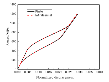
Figure 2: COMPARISON OF PSEUDOELASTIC RESPONSE FOR A SMA BAR PREDICTED BY PROPOSED FINITE STRAIN MODEL AND INFINITESIMAL STRAIN MODEL WITH TRANSFORMATION STRAIN ${H}^{max}=1\%$

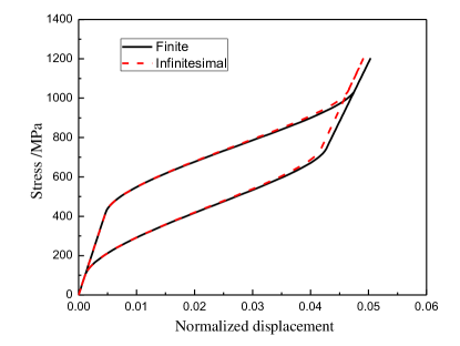
Figure 3: COMPARISON OF PSEUDOELASTIC RESPONSE FOR A SMA BAR PREDICTED BY PROPOSED FINITE STRAIN MODEL AND INFINITESIMAL STRAIN MODEL WITH TRANSFORMATION STRAIN ${H}^{max}=3\%$

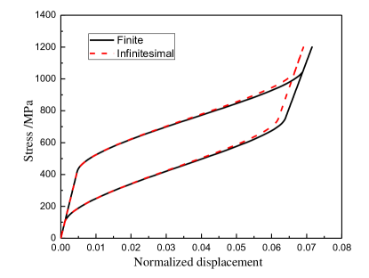
Figure 4: COMPARISON OF PSEUDOELASTIC RESPONSE FOR A SMA BAR PREDICTED BY PROPOSED FINITE STRAIN MODEL AND INFINITESIMAL STRAIN MODEL WITH TRANSFORMATION STRAIN ${H}^{max}=5\%$

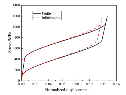
Figure 5: COMPARISON OF PSEUDOELASTIC RESPONSE FOR A SMA BAR PREDICTED BY PROPOSED FINITE STRAIN MODEL AND INFINITESIMAL STRAIN MODEL WITH TRANSFORMATION STRAIN ${H}^{max}=10\%$

As the result is shown in Fig..2, when the maximum transformation is strain $1\%$, the difference of pseudoelastic response curve predicted by the two models is almost negligible. However, with the increasing of maximum transformation strain from $1\%$ to $3\%$, and more to $5\%$ and $10\%$, the difference of predicted pseudoelastic response is becoming predominant. Specifically, with max transformation strain $H^{max}=3\%$ in Fig.3, the difference is becoming perceivable at the end of forward transformation, normalized displacement has larger value predicted by proposed finite strain model in contrast to infinitesimal strain model. This response difference is growing substantial in the cases of $H^{max}$ to be $5\%$ and $10\%$. Since there is no rotation involved here, the difference for the result comes from the fact that infinitesimal strain neglect the higher order terms in strain measure while logarithmic strain used in proposed model doesn’t.

Tube Problem

In this section, a shear problem of a hollow cylindrical SMA torque tube under torsion loading at constant temperature is studied. Referring to Fig.6 for problem schematic, a full size geometry of long hollow cylindrical torque tube is depicted in Fig.6(a). In order to reduce the computational cost, only one small segment tube with length $L$ and inner radius $r$ is chosen for analysis. The segment tube has a geometry ratio of $L/r=2$.

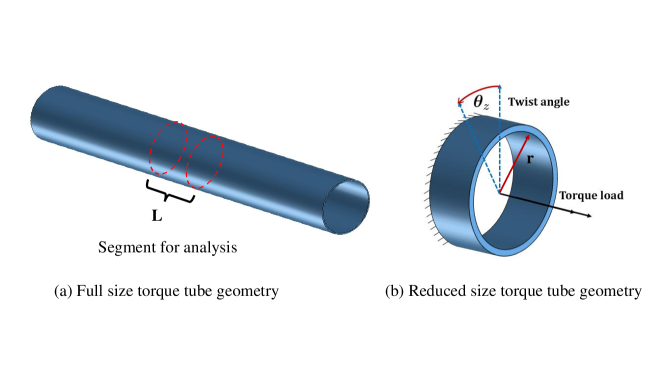
Figure 6: SCHEMATIC FOR THE SHEAR PROBLEM OF HOLLOW CYLINDRICAL SMA TORQUE TUBE

As it is shown in Fig.6(b), the mechanical boundary condition is following: the tube left face is fixed in all degrees of freedom while the right face is subject to a torsion loading through a twist angle $\theta_{z}(t)$ along its longitudinal direction. The loading history is: the twist angle $\theta_{z}(t)$ increases proportionally from zero to a maximum value at $t=0.5$, during which the torque tube undergoes a fully forward phase transformation from austenite phase to detwinned martensite phase. Afterwards, twist angle $\theta_{z}(t)$ proportionally decreases from its peak value to zero, during which the SMA tube experienced a reverse phase transformation from martenite phase to austenite phase. Temperature is kept as a constant value of $360$ K throughout this whole loading process. Material parameters used in this numerical experiment are choosing from Tab.1.

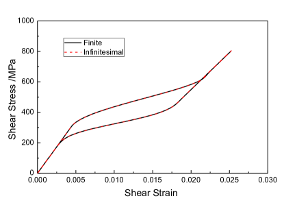
Figure 7: COMPARISON OF PSEUDOELASTIC RESPONSE FOR A SHORT SMA TORSION TUBE PREDICTED BY PROPOSED FINITE STRAIN AND INFINITESIMAL STRAIN MODEL WITH TRANSFORMATION STRAIN ${H}^{max}=1\%$, GEOMETRY RATIO $L/r=2$

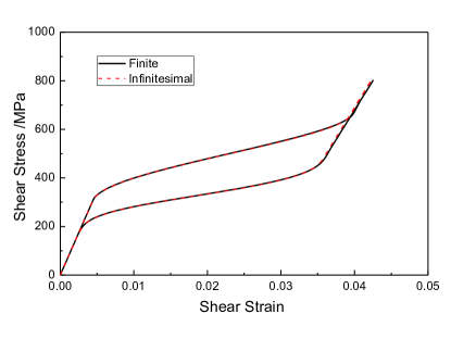
Figure 8: COMPARISON OF PSEUDOELASTIC RESPONSE FOR A SHORT SMA TORSION TUBE PREDICTED BY PROPOSED FINITE STRAIN AND INFINITESIMAL STRAIN MODEL WITH TRANSFORMATION STRAIN ${H}^{max}=3\%$, GEOMETRY RATIO $L/r=2$

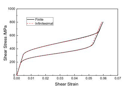
Figure 9: COMPARISON OF PSEUDOELASTIC RESPONSE FOR A SHORT SMA TORSION TUBE PREDICTED BY PROPOSED FINITE STRAIN AND INFINITESIMAL STRAIN MODEL WITH TRANSFORMATION STRAIN ${H}^{max}=5\%$, GEOMETRY RATIO $L/r=2$

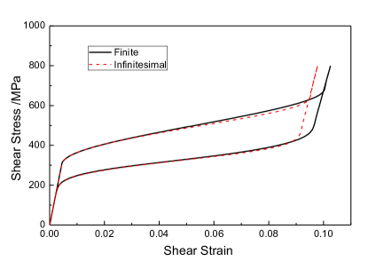
Figure 10: COMPARISON OF PSEUDOELASTIC RESPONSE FOR A SHORT SMA TORSION TUBE PREDICTED BY PROPOSED FINITE STRAIN AND INFINITESIMAL STRAIN MODEL WITH TRANSFORMATION STRAIN ${H}^{max}=10\%$, GEOMETRY RATIO $L/r=2$

It can be observed from the results showing from Fig.7 to Fig.10, although there is no considerable difference on the material response predicted by both models for maximum transformation strain $H^{max}=1\%\sim 3\%$, perceivable difference for maximum transformation strain $H^{max}=5\%$ is showing in Fig.9, and this difference continues to grow substantially as maximum transformation strain increases to $H^{max}=10\%$ in Fig.10. Through the above comparison on the pseudoelastic response for segment torque tube, it is demonstrated that, under large rotations, the difference of predicted material response by proposed finite strain model and infinitesimal model will be perceivable within moderate strain regime of $5\%$, and it continues to grow substantially in large strain regime at $10\%$.

Cyclic Response of SMA Torque Tube

As it was discussed in the section of introduction, based on the additive decomposition in finite deformation theory, a rate form hypoelastic constitutive equation is often seen as stress and strain relationship, in which a objective rate is usually required on the stress tensor in order to meet the principle of objectivity. There are many different objective rates proposed by different researchers along this line, among which several famous ones are Zaremba-Jaumann rate, Green-Naghdi rate and Truesdell rate etc.. However, for a long period of time, rate form hypoelastic constitutive theory has been criticized for its inconsistent choices on objective rates[40], and also the rate form hypoelastic constitutive equation is not able to be integrated to deliver a algebraic constitutive equation, thereby many spurious phenomenons, such as shear stress oscillation, dissipative phenomenon or artificial residual stress are observed in even simple elastic deformation. The aforementioned self-inconsistent issues of hypoelastic constitutive model are resolved by the logarithmic rate proposed by Xiao et al. [30, 31, 29], Bruhns et al.[32, 33, 34], Meyers et al.[35, 36].

In this section, a segment torsion tube is analyzed by proposed finite strain model and its original infinitesimal counterpart with Abaqus NLGEOM (nonlinear geometry) option to extend it for large deformation analysis. The loading conditions and material parameters used are the same as previous segment torsion tube. It should be clear, when the Abaqus NLGEOM option is activated for infinitesimal strain based SMA model during implicit analysis, the strain measure is logarithmic strain and Jaumman rate is the utilized objective rate to capture rotation deformation. As it is mentioned about with objective rates, artificial residual stresses will be introduced by using other objective rates except for the logarithmic one.

Pseudoelastic response of the SMA torque tube are examined by proposed finite strain model and its infinitesimal counterpart with Abaqus NLGEOM option. At the end of the first loading cycle, the Von Mises stress are checked in both cases. As it is shown in Fig.11, the artificial residual stress is almost zero predicted by proposed finite strain model, while the residual stress obtained from infinitesimal model with Abaqus NLGEOM option is around 8 MPa in contrast. The artificial residual stresses from those two cases are summarized in principal components representation at Tab.2.

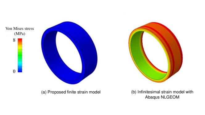
Figure 11: COMPARISON OF ARTIFICIAL RESIDUAL STRESS CONTOUR PREDICTED BY PROPOSED FINITE STRAIN MODEL AND INFINITESIMAL MODEL WITH ABAQUS NLGEOM OPTION FOR A SMA TORQUE TUBE AFTER ONE LOADING CYCLE.

Table 2: ARTIFICIAL RESIDUAL STRESS INTRODUCED FOR SMA TORQUE TUBE AFTER ONE LOADING CYCLE

	Stress Components	Proposed finite strain model	30cmInfinitesimal strain model with
Abaqus NLGEOM
	Principal Max.(MPa)	1.77e-7	4.04
	Principal Mid.(MPa)	1.05e-7	-4.19
	Principal Min.(MPa)	3.22e-8	-4.32

Build on the results for one loading cycle, let us now examine whether this accumulation of artificial residual stresses will continue to grow, and how it will affect the material response of SMAs torque tube under cyclic loadings. Referring to Fig.12 for material response predicted by the infinitesimal model using Abaqus NLGEOM option, it can be seen that there is a clear response shifting from initial to final loading cycle due to the accumulation of artificial residual stress. Specifically, the stress levels required to start the forward phase transformation is decreasing, maximum shear stress achieved is increasing and the shear stress at end of each loading cycle is deviating more and more from the initial zero value. In contrast, material response predicted by proposed finite strain model in Fig.13, the initial material response is nearly overlapping with the material response from subsequent loading cycles.

Figure 12: CYCLIC PSEUDOELASTIC RESPONSE OF A SMA TORQUE TUBE PREDICTED BY INFINITESIMAL MODEL WITH ABAQUS NLGEOM OPTION UNDER 90 CYCLIC LOADINGS

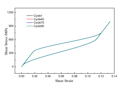
Figure 13: CYCLIC PSEUDOELASTIC RESPONSE OF A SMA TORQUE TUBE PREDICTED BY PROPOSED FINITE STRAIN MODEL UNDER 90 CYCLIC LOADINGS

Based on the results for segment SMA torque tube under cyclic loading, it is demonstrated that, because of the small amount of artificial residual stress introduced by using Abaqus NLGEOM option, the infinitesimal strain based constitutive model for SMAs will predict an shifting, instead of stable, cyclic pseudoelastic response for a torque tube. It is also shown that the proposed finite strain SMA constitutive model, based on logarithmic strain and logarithmic rate, can effectively rule out the effects of artificial residual stress during cyclic loadings. Nevertheless, it is worthy of pointing out for general metallic material within small strain regime during low loading cycles, the amount of artificial residual stresses have quite limited effects on the material response, and it is still a practical and relatively accurate way to utilize the Abaqus NLGEOM option to consider deformation involved with large rotations. At the same time, it is crucial to realized that such undesired artificial stresses need be taken into consideration when the material is undergoing a large number of cyclic loadings, for which a finite strain constitutive model for SMAs based on logarithmic strain and logarithmic rate is indispensible in order to deliver an stable and accurate material response.

CONCLUSION

Based on the infinitesimal strain based constitutive model for shape memory alloys from Lagoudas and coworkers[4, 42], a three dimensional phenomenological constitutive model for martensitic transformation in polycrystalline shape memory alloys considering large strains and large rotations is proposed in this work. Numerical simulations considering basic SMA component geometries, such as a bar and a torque tube under stress induced phase transformation, are performed to test the capabilities of the proposed model. For numerical examples of SMA bar, relatively large discrepancies are observed between the responses predicted by the proposed model and its infinitesimal counterpart when strain is no longer considered small. In the numerical simulations of a SMA torque tube with large rotations, it is demonstrated that the difference of predicted material response will be perceivable in moderate strain regime of $5\%$ and continues to grow substantially in large strain regime at $10\%$. From the results of SMA torque tube under cyclic loading, it has been shown that infinitesimal strain based constitutive model will predict an shifting cyclic pseudoelastic response as a result of the artificial residual stress introduced by using Abaqus NLGEOM option. In comparison, the proposed finite strain SMA constitutive model, based on logarithmic strain and logarithmic rate, can effectively rule out the effects of artificial residual stress during cyclic loadings.

References

- [1] Wheeler, R. W., Hartl, D. J., Chemisky, Y., and Lagoudas, D. C., 2014. “Characterization and modeling of thermo-mechanical fatigue in equiatomic niti actuators”. In ASME 2014 Conference on Smart Materials, Adaptive Structures and Intelligent Systems, American Society of Mechanical Engineers, pp. V002T02A009–V002T02A009.
- [2] Chemisky, Y., Hartl, D. J., and Meraghni, F., 2018. “Three-dimensional constitutive model for structural and functional fatigue of shape memory alloy actuators”. International Journal of Fatigue, 112, pp. 263–278.
- [3] M. Mohajeri, H. Castaneda, D. C. L., 2018. Corrosion monitoring of niti alloy with small-amplitude potential intermodulation technique.
- [4] Boyd, J. G., and Lagoudas, D. C., 1996. “A thermodynamical constitutive model for shape memory materials. part i. the monolithic shape memory alloy”. International Journal of Plasticity, 12(6), pp. 805–842.
- [5] Birman, V., 1997. “Review of mechanics of shape memory alloy structures”. Applied Mechanics Reviews, 50(11), pp. 629–645.
- [6] Raniecki, B., Lexcellent, C., and Tanaka, K., 1992. “Thermodynamic models of pseudoelastic behaviour of shape memory alloys”. Archiv of Mechanics, Archiwum Mechaniki Stosowanej, 44, pp. 261–284.
- [7] Raniecki, B., and Lexcellent, C., 1998. “Thermodynamics of isotropic pseudoelasticity in shape memory alloys”. European Journal of Mechanics-A/Solids, 17(2), pp. 185–205.
- [8] Patoor, E., Lagoudas, D. C., Entchev, P. B., Brinson, L. C., and Gao, X., 2006. “Shape memory alloys, part i: General properties and modeling of single crystals”. Mechanics of materials, 38(5), pp. 391–429.
- [9] Patoor, E., Eberhardt, A., and Berveiller, M., 1996. “Micromechanical modelling of superelasticity in shape memory alloys”. Le Journal de Physique IV, 6(C1), pp. C1–277.
- [10] Hackl, K., and Heinen, R., 2008. “A micromechanical model for pretextured polycrystalline shape-memory alloys including elastic anisotropy”. Continuum Mechanics and Thermodynamics, 19(8), pp. 499–510.
- [11] Levitas, V. I., 1998. “Thermomechanical theory of martensitic phase transformations in inelastic materials”. International Journal of Solids and Structures, 35(9), pp. 889–940.
- [12] Jani, J. M., Leary, M., Subic, A., and Gibson, M. A., 2014. “A review of shape memory alloy research, applications and opportunities”. Materials & Design, 56, pp. 1078–1113.
- [13] Shaw, J. A., 2000. “Simulations of localized thermo-mechanical behavior in a niti shape memory alloy”. International Journal of Plasticity, 16(5), pp. 541–562.
- [14] Wheeler, R. W., Hartl, D. J., Chemisky, Y., and Lagoudas, D. C., 2014. “Characterization and modeling of thermo-mechanical fatigue in equiatomic niti actuators”. In ASME 2014 Conference on Smart Materials, Adaptive Structures and Intelligent Systems, American Society of Mechanical Engineers, pp. V002T02A009–V002T02A009.
- [15] Xu, L., Baxevanis, T., and Lagoudas, D., 2017. “A finite strain constitutive model considering transformation induced plasticity for shape memory alloys under cyclic loading”. In 8th ECCOMAS Thematic Conference on Smart Structures and Materials, pp. 1645–1477.
- [16] Haghgouyan, B., Jape, S., Hayrettin, C., Baxevanis, T., Karaman, I., and Lagoudas, D. C., 2018. “Experimental and numerical investigation of the stable crack growth regime under pseudoelastic loading in shape memory alloys”. In Behavior and Mechanics of Multifunctional Materials and Composites XII, Vol. 10596, International Society for Optics and Photonics, p. 1059612.
- [17] Haghgouyan, B., Hayrettin, C., Baxevanis, T., Karaman, I., and Lagoudas, D. C., 2018. “On the experimental evaluation of the fracture toughness of shape memory alloys”. In TMS Annual Meeting & Exhibition, Springer, pp. 565–573.
- [18] Haghgouyan, B., Shafaghi, N., Aydıner, C. C., and Anlas, G., 2016. “Experimental and computational investigation of the effect of phase transformation on fracture parameters of an sma”. Smart Materials and Structures, 25(7), p. 075010.
- [19] Shafaghi, N., Haghgouyan, B., Aydiner, C. C., and Anlas, G., 2015. “Experimental and computational evaluation of crack-tip displacement field and transformation zone in niti”. Materials Today: Proceedings, 2, pp. S763–S766.
- [20] Auricchio, F., and Taylor, R. L., 1997. “Shape-memory alloys: modelling and numerical simulations of the finite-strain superelastic behavior”. Computer methods in applied mechanics and engineering, 143(1), pp. 175–194.
- [21] Auricchio, F., 2001. “A robust integration-algorithm for a finite-strain shape-memory-alloy superelastic model”. International Journal of plasticity, 17(7), pp. 971–990.
- [22] Arghavani, J., Auricchio, F., and Naghdabadi, R., 2011. “A finite strain kinematic hardening constitutive model based on hencky strain: general framework, solution algorithm and application to shape memory alloys”. International Journal of Plasticity, 27(6), pp. 940–961.
- [23] Arghavani, J., Auricchio, F., Naghdabadi, R., and Reali, A., 2011. “An improved, fully symmetric, finite-strain phenomenological constitutive model for shape memory alloys”. Finite Elements in Analysis and Design, 47(2), pp. 166–174.
- [24] Arghavani, J., Auricchio, F., Naghdabadi, R., Reali, A., and Sohrabpour, S., 2010. “A 3d finite strain phenomenological constitutive model for shape memory alloys considering martensite reorientation”. Continuum Mechanics and Thermodynamics, 22(5), pp. 345–362.
- [25] Thamburaja, P., 2010. “A finite-deformation-based phenomenological theory for shape-memory alloys”. International Journal of Plasticity, 26(8), pp. 1195–1219.
- [26] Thamburaja, P., and Anand, L., 2001. “Polycrystalline shape-memory materials: effect of crystallographic texture”. Journal of the Mechanics and Physics of Solids, 49(4), pp. 709–737.
- [27] Christ, D., and Reese, S., 2009. “A finite element model for shape memory alloys considering thermomechanical couplings at large strains”. International Journal of solids and Structures, 46(20), pp. 3694–3709.
- [28] Reese, S., and Christ, D., 2008. “Finite deformation pseudo-elasticity of shape memory alloys–constitutive modelling and finite element implementation”. International Journal of Plasticity, 24(3), pp. 455–482.
- [29] Xiao, H., Bruhns, O., and Meyers, A., 2006. “Elastoplasticity beyond small deformations”. Acta Mechanica, 182(1-2), pp. 31–111.
- [30] Xiao, H., Bruhns, I. O., and Meyers, I. A., 1997. “Logarithmic strain, logarithmic spin and logarithmic rate”. Acta Mechanica, 124(1-4), pp. 89–105.
- [31] Xiao, H., Bruhns, O., and Meyers, A., 1997. “Hypo-elasticity model based upon the logarithmic stress rate”. Journal of Elasticity, 47(1), pp. 51–68.
- [32] Bruhns, O., Xiao, H., and Meyers, A., 1999. “Self-consistent eulerian rate type elasto-plasticity models based upon the logarithmic stress rate”. International Journal of Plasticity, 15(5), pp. 479–520.
- [33] Bruhns, O., Xiao, H., and Meyers, A., 2001. “Large simple shear and torsion problems in kinematic hardening elasto-plasticity with logarithmic rate”. International journal of solids and structures, 38(48), pp. 8701–8722.
- [34] Bruhns, O., Xiao, H., and Meyers, A., 2001. “A self-consistent eulerian rate type model for finite deformation elastoplasticity with isotropic damage”. International Journal of Solids and Structures, 38(4), pp. 657–683.
- [35] Meyers, A., Xiao, H., and Bruhns, O., 2003. “Elastic stress ratcheting and corotational stress rates”. Tech. Mech, 23, pp. 92–102.
- [36] Meyers, A., Xiao, H., and Bruhns, O., 2006. “Choice of objective rate in single parameter hypoelastic deformation cycles”. Computers & structures, 84(17), pp. 1134–1140.
- [37] Müller, C., and Bruhns, O., 2006. “A thermodynamic finite-strain model for pseudoelastic shape memory alloys”. International Journal of Plasticity, 22(9), pp. 1658–1682.
- [38] Teeriaho, J.-P., 2013. “An extension of a shape memory alloy model for large deformations based on an exactly integrable eulerian rate formulation with changing elastic properties”. International Journal of Plasticity, 43, pp. 153–176.
- [39] Xu, L., Baxevanis, T., and Lagoudas, D. C., 2017. “A finite strain constitutive model for martensitic transformation in shape memory alloys based on logarithmic strain”. In 25th AIAA/AHS Adaptive Structures Conference, p. 0731.
- [40] Simo, J. C., and Hughes, T. J., 2006. Computational inelasticity, Vol. 7. Springer Science & Business Media.
- [41] Khan, A. S., and Huang, S., 1995. Continuum theory of plasticity. John Wiley & Sons.
- [42] Lagoudas, D., Hartl, D., Chemisky, Y., Machado, L., and Popov, P., 2012. “Constitutive model for the numerical analysis of phase transformation in polycrystalline shape memory alloys”. International Journal of Plasticity, 32, pp. 155–183.
- [43] Lagoudas, D. C., 2008. “Shape memory alloys”. Science and Business Media, LLC.