All-Sky Measurement of the Anisotropy of Cosmic Rays at 10 TeV
and Mapping of the Local Interstellar Magnetic Field
A.U. Abeysekara
Department of Physics and Astronomy, University of Utah, Salt Lake City, UT, USA
R. Alfaro
Instituto de Física, Universidad Nacional Autónoma de México, Ciudad de Mexico, Mexico
C. Alvarez
Universidad Autónoma de Chiapas, Tuxtla Gutiérrez, Chiapas, México
R. Arceo
Universidad Autónoma de Chiapas, Tuxtla Gutiérrez, Chiapas, México
J.C. Arteaga-Velázquez
Universidad Michoacana de San Nicolás de Hidalgo, Morelia, Mexico
D. Avila Rojas
Instituto de Física, Universidad Nacional Autónoma de México, Ciudad de Mexico, Mexico
E. Belmont-Moreno
Instituto de Física, Universidad Nacional Autónoma de México, Ciudad de Mexico, Mexico
S.Y. BenZvi
Department of Physics and Astronomy, University of Rochester, Rochester, NY 14627, USA
C. Brisbois
Department of Physics, Michigan Technological University, Houghton, MI, USA
T. Capistrán
Instituto Nacional de Astrofísica, Óptica y Electrónica, Puebla, Mexico
A. Carramiñana
Instituto Nacional de Astrofísica, Óptica y Electrónica, Puebla, Mexico
S. Casanova
Institute of Nuclear Physics Polish Academy of Sciences, PL-31342 IFJ-PAN, Krakow, Poland
U. Cotti
Universidad Michoacana de San Nicolás de Hidalgo, Morelia, Mexico
J. Cotzomi
Facultad de Ciencias Físico Matemáticas, Benemérita Universidad Autónoma de Puebla, Puebla, Mexico
J.C. Díaz-Vélez
Departamento de Física, Centro Universitario de los Valles, Universidad de Guadalajara, Guadalajara, Mexico
Department of Physics and Wisconsin IceCube Particle Astrophysics Center, University of Wisconsin, Madison, WI 53706, USA
C. De León
Facultad de Ciencias Físico Matemáticas, Benemérita Universidad Autónoma de Puebla, Puebla, Mexico
E. De la Fuente
Departamento de Física, Centro Universitario de Ciencias Exactase Ingenierias, Universidad de Guadalajara, Guadalajara, Mexico
S. Dichiara
Instituto de Astronomía, Universidad Nacional Autónoma de México, Ciudad de Mexico, Mexico
M.A. DuVernois
Department of Physics and Wisconsin IceCube Particle Astrophysics Center, University of Wisconsin, Madison, WI 53706, USA
C. Espinoza
Instituto de Física, Universidad Nacional Autónoma de México, Ciudad de Mexico, Mexico
D.W. Fiorino
Department of Physics, University of Maryland, College Park, MD 20742, USA
H. Fleischhack
Department of Physics, Michigan Technological University, Houghton, MI, USA
N. Fraija
Instituto de Astronomía, Universidad Nacional Autónoma de México, Ciudad de Mexico, Mexico
A. Galván-Gámez
Instituto de Astronomía, Universidad Nacional Autónoma de México, Ciudad de Mexico, Mexico
J.A. García-González
Instituto de Física, Universidad Nacional Autónoma de México, Ciudad de Mexico, Mexico
M.M. González
Instituto de Astronomía, Universidad Nacional Autónoma de México, Ciudad de Mexico, Mexico
J.A. Goodman
Department of Physics, University of Maryland, College Park, MD 20742, USA
Z. Hampel-Arias
Department of Physics and Wisconsin IceCube Particle Astrophysics Center, University of Wisconsin, Madison, WI 53706, USA
Inter-university Institute for High Energies, Université Libre de Bruxelles, Bruxelles, Belgium
J.P. Harding
Physics Division, Los Alamos National Laboratory, Los Alamos, NM, USA
S. Hernandez
Instituto de Física, Universidad Nacional Autónoma de México, Ciudad de Mexico, Mexico
B. Hona
Department of Physics, Michigan Technological University, Houghton, MI, USA
F. Hueyotl-Zahuantitla
Universidad Autónoma de Chiapas, Tuxtla Gutiérrez, Chiapas, México
A. Iriarte
Instituto de Astronomía, Universidad Nacional Autónoma de México, Ciudad de Mexico, Mexico
A. Jardin-Blicq
Max-Planck Institute for Nuclear Physics, 69117 Heidelberg, Germany
V. Joshi
Max-Planck Institute for Nuclear Physics, 69117 Heidelberg, Germany
A. Lara
Instituto de Geofísica, Universidad Nacional Autónoma de México, Ciudad de Mexico, Mexico
H. León Vargas
Instituto de Física, Universidad Nacional Autónoma de México, Ciudad de Mexico, Mexico
G. Luis-Raya
Universidad Politecnica de Pachuca, Pachuca, Hgo, Mexico
K. Malone
Department of Physics, Pennsylvania State University, University Park, PA 16802, USA
S.S. Marinelli
Department of Physics and Astronomy, Michigan State University, East Lansing, MI 48824, USA
J. Martínez-Castro
Centro de Investigación en Computación, Instituto Politécnico Nacional, México City, México.
O. Martinez
Facultad de Ciencias Físico Matemáticas, Benemérita Universidad Autónoma de Puebla, Puebla, Mexico
J.A. Matthews
Departmentof Physics and Astronomy, University of New Mexico, Albuquerque, NM, USA
P. Miranda-Romagnoli
Universidad Autónoma del Estado de Hidalgo, Pachuca, Mexico
E. Moreno
Facultad de Ciencias Físico Matemáticas, Benemérita Universidad Autónoma de Puebla, Puebla, Mexico
M. Mostafá
Department of Physics, Pennsylvania State University, University Park, PA 16802, USA
L. Nellen
Instituto de Ciencias Nucleares, Universidad Nacional Autónoma de Mexico, Ciudad de Mexico, Mexico
M. Newbold
Department of Physics and Astronomy, University of Utah, Salt Lake City, UT, USA
M.U. Nisa
Department of Physics and Astronomy, University of Rochester, Rochester, NY 14627, USA
R. Noriega-Papaqui
Universidad Autónoma del Estado de Hidalgo, Pachuca, Mexico
E.G. Pérez-Pérez
Universidad Politecnica de Pachuca, Pachuca, Hgo, Mexico
J. Pretz
Department of Physics, Pennsylvania State University, University Park, PA 16802, USA
Z. Ren
Departmentof Physics and Astronomy, University of New Mexico, Albuquerque, NM, USA
C.D. Rho
Department of Physics and Astronomy, University of Rochester, Rochester, NY 14627, USA
C. Rivière
Department of Physics, University of Maryland, College Park, MD 20742, USA
D. Rosa-González
Instituto Nacional de Astrofísica, Óptica y Electrónica, Puebla, Mexico
M. Rosenberg
Department of Physics, Pennsylvania State University, University Park, PA 16802, USA
H. Salazar
Facultad de Ciencias Físico Matemáticas, Benemérita Universidad Autónoma de Puebla, Puebla, Mexico
F. Salesa Greus
Institute of Nuclear Physics Polish Academy of Sciences, PL-31342 IFJ-PAN, Krakow, Poland
A. Sandoval
Instituto de Física, Universidad Nacional Autónoma de México, Ciudad de Mexico, Mexico
M. Schneider
Department of Physics, University of Maryland, College Park, MD 20742, USA
H. Schoorlemmer
Max-Planck Institute for Nuclear Physics, 69117 Heidelberg, Germany
G. Sinnis
Physics Division, Los Alamos National Laboratory, Los Alamos, NM, USA
A.J. Smith
Department of Physics, University of Maryland, College Park, MD 20742, USA
P. Surajbali
Max-Planck Institute for Nuclear Physics, 69117 Heidelberg, Germany
I. Taboada
School of Physics and Center for Relativistic Astrophysics, Georgia Institute of Technology, Atlanta, GA 30332, USA
K. Tollefson
Department of Physics and Astronomy, Michigan State University, East Lansing, MI 48824, USA
I. Torres
Instituto Nacional de Astrofísica, Óptica y Electrónica, Puebla, Mexico
L. Villaseñor
Facultad de Ciencias Físico Matemáticas, Benemérita Universidad Autónoma de Puebla, Puebla, Mexico
T. Weisgarber
Department of Physics and Wisconsin IceCube Particle Astrophysics Center, University of Wisconsin, Madison, WI 53706, USA
J. Wood
Department of Physics and Wisconsin IceCube Particle Astrophysics Center, University of Wisconsin, Madison, WI 53706, USA
A. Zepeda
Physics Department, Centro de Investigacion y de Estudios Avanzados del IPN, Mexico City, DF, Mexico
H. Zhou
Physics Division, Los Alamos National Laboratory, Los Alamos, NM, USA
J.D. Álvarez
Universidad Michoacana de San Nicolás de Hidalgo, Morelia, Mexico
M. G. Aartsen
Department of Physics and Astronomy, University of Canterbury, Private Bag 4800, Christchurch, New Zealand
M. Ackermann
DESY, D-15738 Zeuthen, Germany
J. Adams
Department of Physics and Astronomy, University of Canterbury, Private Bag 4800, Christchurch, New Zealand
J. A. Aguilar
Université Libre de Bruxelles, Science Faculty CP230, B-1050 Brussels, Belgium
M. Ahlers
Niels Bohr Institute, University of Copenhagen, DK-2100 Copenhagen, Denmark
M. Ahrens
Oskar Klein Centre and Department of Physics, Stockholm University, SE-10691 Stockholm, Sweden
D. Altmann
Erlangen Centre for Astroparticle Physics, Friedrich-Alexander-Universität Erlangen-Nürnberg, D-91058 Erlangen, Germany
K. Andeen
Department of Physics, Marquette University, Milwaukee, WI, 53201, USA
T. Anderson
Department of Physics, Pennsylvania State University, University Park, PA 16802, USA
I. Ansseau
Université Libre de Bruxelles, Science Faculty CP230, B-1050 Brussels, Belgium
G. Anton
Erlangen Centre for Astroparticle Physics, Friedrich-Alexander-Universität Erlangen-Nürnberg, D-91058 Erlangen, Germany
C. Argüelles
Department of Physics, Massachusetts Institute of Technology, Cambridge, MA 02139, USA
J. Auffenberg
III. Physikalisches Institut, RWTH Aachen University, D-52056 Aachen, Germany
S. Axani
Department of Physics, Massachusetts Institute of Technology, Cambridge, MA 02139, USA
P. Backes
III. Physikalisches Institut, RWTH Aachen University, D-52056 Aachen, Germany
H. Bagherpour
Department of Physics and Astronomy, University of Canterbury, Private Bag 4800, Christchurch, New Zealand
X. Bai
Physics Department, South Dakota School of Mines and Technology, Rapid City, SD 57701, USA
A. Barbano
Département de physique nucléaire et corpusculaire, Université de Genève, CH-1211 Genève, Switzerland
J. P. Barron
Department of Physics, University of Alberta, Edmonton, Alberta, Canada T6G 2E1
S. W. Barwick
Department of Physics and Astronomy, University of California, Irvine, CA 92697, USA
V. Baum
Institute of Physics, University of Mainz, Staudinger Weg 7, D-55099 Mainz, Germany
R. Bay
Department of Physics, University of California, Berkeley, CA 94720, USA
J. J. Beatty
Department of Physics and Center for Cosmology and Astro-Particle Physics, Ohio State University, Columbus, OH 43210, USA
Department of Astronomy, Ohio State University, Columbus, OH 43210, USA
J. Becker Tjus
Fakultät für Physik & Astronomie, Ruhr-Universität Bochum, D-44780 Bochum, Germany
K.-H. Becker
Department of Physics, University of Wuppertal, D-42119 Wuppertal, Germany
S. BenZvi
Department of Physics and Astronomy, University of Rochester, Rochester, NY 14627, USA
D. Berley
Department of Physics, University of Maryland, College Park, MD 20742, USA
E. Bernardini
DESY, D-15738 Zeuthen, Germany
D. Z. Besson
Department of Physics and Astronomy, University of Kansas, Lawrence, KS 66045, USA
G. Binder
Lawrence Berkeley National Laboratory, Berkeley, CA 94720, USA
Department of Physics, University of California, Berkeley, CA 94720, USA
D. Bindig
Department of Physics, University of Wuppertal, D-42119 Wuppertal, Germany
E. Blaufuss
Department of Physics, University of Maryland, College Park, MD 20742, USA
S. Blot
DESY, D-15738 Zeuthen, Germany
C. Bohm
Oskar Klein Centre and Department of Physics, Stockholm University, SE-10691 Stockholm, Sweden
M. Börner
Department of Physics, TU Dortmund University, D-44221 Dortmund, Germany
F. Bos
Fakultät für Physik & Astronomie, Ruhr-Universität Bochum, D-44780 Bochum, Germany
S. Böser
Institute of Physics, University of Mainz, Staudinger Weg 7, D-55099 Mainz, Germany
O. Botner
Department of Physics and Astronomy, Uppsala University, Box 516, S-75120 Uppsala, Sweden
E. Bourbeau
Niels Bohr Institute, University of Copenhagen, DK-2100 Copenhagen, Denmark
J. Bourbeau
Department of Physics and Wisconsin IceCube Particle Astrophysics Center, University of Wisconsin, Madison, WI 53706, USA
F. Bradascio
DESY, D-15738 Zeuthen, Germany
J. Braun
Department of Physics and Wisconsin IceCube Particle Astrophysics Center, University of Wisconsin, Madison, WI 53706, USA
H.-P. Bretz
DESY, D-15738 Zeuthen, Germany
S. Bron
Département de physique nucléaire et corpusculaire, Université de Genève, CH-1211 Genève, Switzerland
J. Brostean-Kaiser
DESY, D-15738 Zeuthen, Germany
A. Burgman
Department of Physics and Astronomy, Uppsala University, Box 516, S-75120 Uppsala, Sweden
R. S. Busse
Department of Physics and Wisconsin IceCube Particle Astrophysics Center, University of Wisconsin, Madison, WI 53706, USA
T. Carver
Département de physique nucléaire et corpusculaire, Université de Genève, CH-1211 Genève, Switzerland
E. Cheung
Department of Physics, University of Maryland, College Park, MD 20742, USA
D. Chirkin
Department of Physics and Wisconsin IceCube Particle Astrophysics Center, University of Wisconsin, Madison, WI 53706, USA
K. Clark
SNOLAB, 1039 Regional Road 24, Creighton Mine 9, Lively, ON, Canada P3Y 1N2
L. Classen
Institut für Kernphysik, Westfälische Wilhelms-Universität Münster, D-48149 Münster, Germany
G. H. Collin
Department of Physics, Massachusetts Institute of Technology, Cambridge, MA 02139, USA
J. M. Conrad
Department of Physics, Massachusetts Institute of Technology, Cambridge, MA 02139, USA
P. Coppin
Vrije Universiteit Brussel (VUB), Dienst ELEM, B-1050 Brussels, Belgium
P. Correa
Vrije Universiteit Brussel (VUB), Dienst ELEM, B-1050 Brussels, Belgium
D. F. Cowen
Department of Physics, Pennsylvania State University, University Park, PA 16802, USA
Department of Astronomy and Astrophysics, Pennsylvania State University, University Park, PA 16802, USA
R. Cross
Department of Physics and Astronomy, University of Rochester, Rochester, NY 14627, USA
P. Dave
School of Physics and Center for Relativistic Astrophysics, Georgia Institute of Technology, Atlanta, GA 30332, USA
M. Day
Department of Physics and Wisconsin IceCube Particle Astrophysics Center, University of Wisconsin, Madison, WI 53706, USA
J. P. A. M. de André
Department of Physics and Astronomy, Michigan State University, East Lansing, MI 48824, USA
C. De Clercq
Vrije Universiteit Brussel (VUB), Dienst ELEM, B-1050 Brussels, Belgium
J. J. DeLaunay
Department of Physics, Pennsylvania State University, University Park, PA 16802, USA
H. Dembinski
Bartol Research Institute and Department of Physics and Astronomy, University of Delaware, Newark, DE 19716, USA
K. Deoskar
Oskar Klein Centre and Department of Physics, Stockholm University, SE-10691 Stockholm, Sweden
S. De Ridder
Department of Physics and Astronomy, University of Gent, B-9000 Gent, Belgium
P. Desiati
Department of Physics and Wisconsin IceCube Particle Astrophysics Center, University of Wisconsin, Madison, WI 53706, USA
K. D. de Vries
Vrije Universiteit Brussel (VUB), Dienst ELEM, B-1050 Brussels, Belgium
G. de Wasseige
Vrije Universiteit Brussel (VUB), Dienst ELEM, B-1050 Brussels, Belgium
M. de With
Institut für Physik, Humboldt-Universität zu Berlin, D-12489 Berlin, Germany
T. DeYoung
Department of Physics and Astronomy, Michigan State University, East Lansing, MI 48824, USA
J. C. Díaz-Vélez
Departamento de Física, Centro Universitario de los Valles, Universidad de Guadalajara, Guadalajara, Mexico
Department of Physics and Wisconsin IceCube Particle Astrophysics Center, University of Wisconsin, Madison, WI 53706, USA
H. Dujmovic
Department of Physics, Sungkyunkwan University, Suwon 440-746, Korea
M. Dunkman
Department of Physics, Pennsylvania State University, University Park, PA 16802, USA
E. Dvorak
Physics Department, South Dakota School of Mines and Technology, Rapid City, SD 57701, USA
B. Eberhardt
Institute of Physics, University of Mainz, Staudinger Weg 7, D-55099 Mainz, Germany
T. Ehrhardt
Institute of Physics, University of Mainz, Staudinger Weg 7, D-55099 Mainz, Germany
B. Eichmann
Fakultät für Physik & Astronomie, Ruhr-Universität Bochum, D-44780 Bochum, Germany
P. Eller
Department of Physics, Pennsylvania State University, University Park, PA 16802, USA
P. A. Evenson
Bartol Research Institute and Department of Physics and Astronomy, University of Delaware, Newark, DE 19716, USA
S. Fahey
Department of Physics and Wisconsin IceCube Particle Astrophysics Center, University of Wisconsin, Madison, WI 53706, USA
A. R. Fazely
Department of Physics, Southern University, Baton Rouge, LA 70813, USA
J. Felde
Department of Physics, University of Maryland, College Park, MD 20742, USA
K. Filimonov
Department of Physics, University of California, Berkeley, CA 94720, USA
C. Finley
Oskar Klein Centre and Department of Physics, Stockholm University, SE-10691 Stockholm, Sweden
A. Franckowiak
DESY, D-15738 Zeuthen, Germany
E. Friedman
Department of Physics, University of Maryland, College Park, MD 20742, USA
A. Fritz
Institute of Physics, University of Mainz, Staudinger Weg 7, D-55099 Mainz, Germany
T. K. Gaisser
Bartol Research Institute and Department of Physics and Astronomy, University of Delaware, Newark, DE 19716, USA
J. Gallagher
Department of Astronomy, University of Wisconsin, Madison, WI 53706, USA
E. Ganster
III. Physikalisches Institut, RWTH Aachen University, D-52056 Aachen, Germany
S. Garrappa
DESY, D-15738 Zeuthen, Germany
L. Gerhardt
Lawrence Berkeley National Laboratory, Berkeley, CA 94720, USA
K. Ghorbani
Department of Physics and Wisconsin IceCube Particle Astrophysics Center, University of Wisconsin, Madison, WI 53706, USA
W. Giang
Department of Physics, University of Alberta, Edmonton, Alberta, Canada T6G 2E1
T. Glauch
Physik-department, Technische Universität München, D-85748 Garching, Germany
T. Glüsenkamp
Erlangen Centre for Astroparticle Physics, Friedrich-Alexander-Universität Erlangen-Nürnberg, D-91058 Erlangen, Germany
A. Goldschmidt
Lawrence Berkeley National Laboratory, Berkeley, CA 94720, USA
J. G. Gonzalez
Bartol Research Institute and Department of Physics and Astronomy, University of Delaware, Newark, DE 19716, USA
D. Grant
Department of Physics, University of Alberta, Edmonton, Alberta, Canada T6G 2E1
Z. Griffith
Department of Physics and Wisconsin IceCube Particle Astrophysics Center, University of Wisconsin, Madison, WI 53706, USA
C. Haack
III. Physikalisches Institut, RWTH Aachen University, D-52056 Aachen, Germany
A. Hallgren
Department of Physics and Astronomy, Uppsala University, Box 516, S-75120 Uppsala, Sweden
L. Halve
III. Physikalisches Institut, RWTH Aachen University, D-52056 Aachen, Germany
F. Halzen
Department of Physics and Wisconsin IceCube Particle Astrophysics Center, University of Wisconsin, Madison, WI 53706, USA
K. Hanson
Department of Physics and Wisconsin IceCube Particle Astrophysics Center, University of Wisconsin, Madison, WI 53706, USA
D. Hebecker
Institut für Physik, Humboldt-Universität zu Berlin, D-12489 Berlin, Germany
D. Heereman
Université Libre de Bruxelles, Science Faculty CP230, B-1050 Brussels, Belgium
K. Helbing
Department of Physics, University of Wuppertal, D-42119 Wuppertal, Germany
R. Hellauer
Department of Physics, University of Maryland, College Park, MD 20742, USA
S. Hickford
Department of Physics, University of Wuppertal, D-42119 Wuppertal, Germany
J. Hignight
Department of Physics and Astronomy, Michigan State University, East Lansing, MI 48824, USA
G. C. Hill
Department of Physics, University of Adelaide, Adelaide, 5005, Australia
K. D. Hoffman
Department of Physics, University of Maryland, College Park, MD 20742, USA
R. Hoffmann
Department of Physics, University of Wuppertal, D-42119 Wuppertal, Germany
T. Hoinka
Department of Physics, TU Dortmund University, D-44221 Dortmund, Germany
B. Hokanson-Fasig
Department of Physics and Wisconsin IceCube Particle Astrophysics Center, University of Wisconsin, Madison, WI 53706, USA
K. Hoshina
Department of Physics and Wisconsin IceCube Particle Astrophysics Center, University of Wisconsin, Madison, WI 53706, USA
F. Huang
Department of Physics, Pennsylvania State University, University Park, PA 16802, USA
M. Huber
Physik-department, Technische Universität München, D-85748 Garching, Germany
K. Hultqvist
Oskar Klein Centre and Department of Physics, Stockholm University, SE-10691 Stockholm, Sweden
M. Hünnefeld
Department of Physics, TU Dortmund University, D-44221 Dortmund, Germany
R. Hussain
Department of Physics and Wisconsin IceCube Particle Astrophysics Center, University of Wisconsin, Madison, WI 53706, USA
S. In
Department of Physics, Sungkyunkwan University, Suwon 440-746, Korea
N. Iovine
Université Libre de Bruxelles, Science Faculty CP230, B-1050 Brussels, Belgium
A. Ishihara
Department of Physics and Institute for Global Prominent Research, Chiba University, Chiba 263-8522, Japan
E. Jacobi
DESY, D-15738 Zeuthen, Germany
G. S. Japaridze
CTSPS, Clark-Atlanta University, Atlanta, GA 30314, USA
M. Jeong
Department of Physics, Sungkyunkwan University, Suwon 440-746, Korea
K. Jero
Department of Physics and Wisconsin IceCube Particle Astrophysics Center, University of Wisconsin, Madison, WI 53706, USA
B. J. P. Jones
Department of Physics, University of Texas at Arlington, 502 Yates St., Science Hall Rm 108, Box 19059, Arlington, TX 76019, USA
P. Kalaczynski
III. Physikalisches Institut, RWTH Aachen University, D-52056 Aachen, Germany
W. Kang
Department of Physics, Sungkyunkwan University, Suwon 440-746, Korea
A. Kappes
Institut für Kernphysik, Westfälische Wilhelms-Universität Münster, D-48149 Münster, Germany
D. Kappesser
Institute of Physics, University of Mainz, Staudinger Weg 7, D-55099 Mainz, Germany
T. Karg
DESY, D-15738 Zeuthen, Germany
A. Karle
Department of Physics and Wisconsin IceCube Particle Astrophysics Center, University of Wisconsin, Madison, WI 53706, USA
U. Katz
Erlangen Centre for Astroparticle Physics, Friedrich-Alexander-Universität Erlangen-Nürnberg, D-91058 Erlangen, Germany
M. Kauer
Department of Physics and Wisconsin IceCube Particle Astrophysics Center, University of Wisconsin, Madison, WI 53706, USA
A. Keivani
Department of Physics, Pennsylvania State University, University Park, PA 16802, USA
J. L. Kelley
Department of Physics and Wisconsin IceCube Particle Astrophysics Center, University of Wisconsin, Madison, WI 53706, USA
A. Kheirandish
Department of Physics and Wisconsin IceCube Particle Astrophysics Center, University of Wisconsin, Madison, WI 53706, USA
J. Kim
Department of Physics, Sungkyunkwan University, Suwon 440-746, Korea
T. Kintscher
DESY, D-15738 Zeuthen, Germany
J. Kiryluk
Department of Physics and Astronomy, Stony Brook University, Stony Brook, NY 11794-3800, USA
T. Kittler
Erlangen Centre for Astroparticle Physics, Friedrich-Alexander-Universität Erlangen-Nürnberg, D-91058 Erlangen, Germany
S. R. Klein
Lawrence Berkeley National Laboratory, Berkeley, CA 94720, USA
Department of Physics, University of California, Berkeley, CA 94720, USA
R. Koirala
Bartol Research Institute and Department of Physics and Astronomy, University of Delaware, Newark, DE 19716, USA
H. Kolanoski
Institut für Physik, Humboldt-Universität zu Berlin, D-12489 Berlin, Germany
L. Köpke
Institute of Physics, University of Mainz, Staudinger Weg 7, D-55099 Mainz, Germany
C. Kopper
Department of Physics, University of Alberta, Edmonton, Alberta, Canada T6G 2E1
S. Kopper
Department of Physics and Astronomy, University of Alabama, Tuscaloosa, AL 35487, USA
D. J. Koskinen
Niels Bohr Institute, University of Copenhagen, DK-2100 Copenhagen, Denmark
M. Kowalski
Institut für Physik, Humboldt-Universität zu Berlin, D-12489 Berlin, Germany
DESY, D-15738 Zeuthen, Germany
K. Krings
Physik-department, Technische Universität München, D-85748 Garching, Germany
M. Kroll
Fakultät für Physik & Astronomie, Ruhr-Universität Bochum, D-44780 Bochum, Germany
G. Krückl
Institute of Physics, University of Mainz, Staudinger Weg 7, D-55099 Mainz, Germany
S. Kunwar
DESY, D-15738 Zeuthen, Germany
N. Kurahashi
Department of Physics, Drexel University, 3141 Chestnut Street, Philadelphia, PA 19104, USA
A. Kyriacou
Department of Physics, University of Adelaide, Adelaide, 5005, Australia
M. Labare
Department of Physics and Astronomy, University of Gent, B-9000 Gent, Belgium
J. L. Lanfranchi
Department of Physics, Pennsylvania State University, University Park, PA 16802, USA
M. J. Larson
Niels Bohr Institute, University of Copenhagen, DK-2100 Copenhagen, Denmark
F. Lauber
Department of Physics, University of Wuppertal, D-42119 Wuppertal, Germany
K. Leonard
Department of Physics and Wisconsin IceCube Particle Astrophysics Center, University of Wisconsin, Madison, WI 53706, USA
M. Leuermann
III. Physikalisches Institut, RWTH Aachen University, D-52056 Aachen, Germany
Q. R. Liu
Department of Physics and Wisconsin IceCube Particle Astrophysics Center, University of Wisconsin, Madison, WI 53706, USA
E. Lohfink
Institute of Physics, University of Mainz, Staudinger Weg 7, D-55099 Mainz, Germany
C. J. Lozano Mariscal
Institut für Kernphysik, Westfälische Wilhelms-Universität Münster, D-48149 Münster, Germany
L. Lu
Department of Physics and Institute for Global Prominent Research, Chiba University, Chiba 263-8522, Japan
J. Lünemann
Vrije Universiteit Brussel (VUB), Dienst ELEM, B-1050 Brussels, Belgium
W. Luszczak
Department of Physics and Wisconsin IceCube Particle Astrophysics Center, University of Wisconsin, Madison, WI 53706, USA
J. Madsen
Department of Physics, University of Wisconsin, River Falls, WI 54022, USA
G. Maggi
Vrije Universiteit Brussel (VUB), Dienst ELEM, B-1050 Brussels, Belgium
K. B. M. Mahn
Department of Physics and Astronomy, Michigan State University, East Lansing, MI 48824, USA
Y. Makino
Department of Physics and Institute for Global Prominent Research, Chiba University, Chiba 263-8522, Japan
S. Mancina
Department of Physics and Wisconsin IceCube Particle Astrophysics Center, University of Wisconsin, Madison, WI 53706, USA
I. C. Mariş
Université Libre de Bruxelles, Science Faculty CP230, B-1050 Brussels, Belgium
R. Maruyama
Department of Physics, Yale University, New Haven, CT 06520, USA
K. Mase
Department of Physics and Institute for Global Prominent Research, Chiba University, Chiba 263-8522, Japan
R. Maunu
Department of Physics, University of Maryland, College Park, MD 20742, USA
K. Meagher
Université Libre de Bruxelles, Science Faculty CP230, B-1050 Brussels, Belgium
M. Medici
Niels Bohr Institute, University of Copenhagen, DK-2100 Copenhagen, Denmark
M. Meier
Department of Physics, TU Dortmund University, D-44221 Dortmund, Germany
T. Menne
Department of Physics, TU Dortmund University, D-44221 Dortmund, Germany
G. Merino
Department of Physics and Wisconsin IceCube Particle Astrophysics Center, University of Wisconsin, Madison, WI 53706, USA
T. Meures
Université Libre de Bruxelles, Science Faculty CP230, B-1050 Brussels, Belgium
S. Miarecki
Lawrence Berkeley National Laboratory, Berkeley, CA 94720, USA
Department of Physics, University of California, Berkeley, CA 94720, USA
J. Micallef
Department of Physics and Astronomy, Michigan State University, East Lansing, MI 48824, USA
G. Momenté
Institute of Physics, University of Mainz, Staudinger Weg 7, D-55099 Mainz, Germany
T. Montaruli
Département de physique nucléaire et corpusculaire, Université de Genève, CH-1211 Genève, Switzerland
R. W. Moore
Department of Physics, University of Alberta, Edmonton, Alberta, Canada T6G 2E1
M. Moulai
Department of Physics, Massachusetts Institute of Technology, Cambridge, MA 02139, USA
R. Nagai
Department of Physics and Institute for Global Prominent Research, Chiba University, Chiba 263-8522, Japan
R. Nahnhauer
DESY, D-15738 Zeuthen, Germany
P. Nakarmi
Department of Physics and Astronomy, University of Alabama, Tuscaloosa, AL 35487, USA
U. Naumann
Department of Physics, University of Wuppertal, D-42119 Wuppertal, Germany
G. Neer
Department of Physics and Astronomy, Michigan State University, East Lansing, MI 48824, USA
H. Niederhausen
Department of Physics and Astronomy, Stony Brook University, Stony Brook, NY 11794-3800, USA
S. C. Nowicki
Department of Physics, University of Alberta, Edmonton, Alberta, Canada T6G 2E1
D. R. Nygren
Lawrence Berkeley National Laboratory, Berkeley, CA 94720, USA
A. Obertacke Pollmann
Department of Physics, University of Wuppertal, D-42119 Wuppertal, Germany
A. Olivas
Department of Physics, University of Maryland, College Park, MD 20742, USA
A. O’Murchadha
Université Libre de Bruxelles, Science Faculty CP230, B-1050 Brussels, Belgium
E. O’Sullivan
Oskar Klein Centre and Department of Physics, Stockholm University, SE-10691 Stockholm, Sweden
T. Palczewski
Lawrence Berkeley National Laboratory, Berkeley, CA 94720, USA
Department of Physics, University of California, Berkeley, CA 94720, USA
H. Pandya
Bartol Research Institute and Department of Physics and Astronomy, University of Delaware, Newark, DE 19716, USA
D. V. Pankova
Department of Physics, Pennsylvania State University, University Park, PA 16802, USA
P. Peiffer
Institute of Physics, University of Mainz, Staudinger Weg 7, D-55099 Mainz, Germany
J. A. Pepper
Department of Physics and Astronomy, University of Alabama, Tuscaloosa, AL 35487, USA
C. Pérez de los Heros
Department of Physics and Astronomy, Uppsala University, Box 516, S-75120 Uppsala, Sweden
D. Pieloth
Department of Physics, TU Dortmund University, D-44221 Dortmund, Germany
E. Pinat
Université Libre de Bruxelles, Science Faculty CP230, B-1050 Brussels, Belgium
A. Pizzuto
Department of Physics and Wisconsin IceCube Particle Astrophysics Center, University of Wisconsin, Madison, WI 53706, USA
M. Plum
Department of Physics, Marquette University, Milwaukee, WI, 53201, USA
P. B. Price
Department of Physics, University of California, Berkeley, CA 94720, USA
G. T. Przybylski
Lawrence Berkeley National Laboratory, Berkeley, CA 94720, USA
C. Raab
Université Libre de Bruxelles, Science Faculty CP230, B-1050 Brussels, Belgium
M. Rameez
Niels Bohr Institute, University of Copenhagen, DK-2100 Copenhagen, Denmark
L. Rauch
DESY, D-15738 Zeuthen, Germany
K. Rawlins
Department of Physics and Astronomy, University of Alaska Anchorage, 3211 Providence Dr., Anchorage, AK 99508, USA
I. C. Rea
Physik-department, Technische Universität München, D-85748 Garching, Germany
R. Reimann
III. Physikalisches Institut, RWTH Aachen University, D-52056 Aachen, Germany
B. Relethford
Department of Physics, Drexel University, 3141 Chestnut Street, Philadelphia, PA 19104, USA
G. Renzi
Université Libre de Bruxelles, Science Faculty CP230, B-1050 Brussels, Belgium
E. Resconi
Physik-department, Technische Universität München, D-85748 Garching, Germany
W. Rhode
Department of Physics, TU Dortmund University, D-44221 Dortmund, Germany
M. Richman
Department of Physics, Drexel University, 3141 Chestnut Street, Philadelphia, PA 19104, USA
S. Robertson
Lawrence Berkeley National Laboratory, Berkeley, CA 94720, USA
M. Rongen
III. Physikalisches Institut, RWTH Aachen University, D-52056 Aachen, Germany
C. Rott
Department of Physics, Sungkyunkwan University, Suwon 440-746, Korea
T. Ruhe
Department of Physics, TU Dortmund University, D-44221 Dortmund, Germany
D. Ryckbosch
Department of Physics and Astronomy, University of Gent, B-9000 Gent, Belgium
D. Rysewyk
Department of Physics and Astronomy, Michigan State University, East Lansing, MI 48824, USA
I. Safa
Department of Physics and Wisconsin IceCube Particle Astrophysics Center, University of Wisconsin, Madison, WI 53706, USA
S. E. Sanchez Herrera
Department of Physics, University of Alberta, Edmonton, Alberta, Canada T6G 2E1
A. Sandrock
Department of Physics, TU Dortmund University, D-44221 Dortmund, Germany
J. Sandroos
Institute of Physics, University of Mainz, Staudinger Weg 7, D-55099 Mainz, Germany
M. Santander
Department of Physics and Astronomy, University of Alabama, Tuscaloosa, AL 35487, USA
S. Sarkar
Niels Bohr Institute, University of Copenhagen, DK-2100 Copenhagen, Denmark
Department of Physics, University of Oxford, 1 Keble Road, Oxford OX1 3NP, UK
S. Sarkar
Department of Physics, University of Alberta, Edmonton, Alberta, Canada T6G 2E1
K. Satalecka
DESY, D-15738 Zeuthen, Germany
M. Schaufel
III. Physikalisches Institut, RWTH Aachen University, D-52056 Aachen, Germany
P. Schlunder
Department of Physics, TU Dortmund University, D-44221 Dortmund, Germany
T. Schmidt
Department of Physics, University of Maryland, College Park, MD 20742, USA
A. Schneider
Department of Physics and Wisconsin IceCube Particle Astrophysics Center, University of Wisconsin, Madison, WI 53706, USA
J. Schneider
Erlangen Centre for Astroparticle Physics, Friedrich-Alexander-Universität Erlangen-Nürnberg, D-91058 Erlangen, Germany
S. Schöneberg
Fakultät für Physik & Astronomie, Ruhr-Universität Bochum, D-44780 Bochum, Germany
L. Schumacher
III. Physikalisches Institut, RWTH Aachen University, D-52056 Aachen, Germany
S. Sclafani
Department of Physics, Drexel University, 3141 Chestnut Street, Philadelphia, PA 19104, USA
D. Seckel
Bartol Research Institute and Department of Physics and Astronomy, University of Delaware, Newark, DE 19716, USA
S. Seunarine
Department of Physics, University of Wisconsin, River Falls, WI 54022, USA
J. Soedingrekso
Department of Physics, TU Dortmund University, D-44221 Dortmund, Germany
D. Soldin
Bartol Research Institute and Department of Physics and Astronomy, University of Delaware, Newark, DE 19716, USA
M. Song
Department of Physics, University of Maryland, College Park, MD 20742, USA
G. M. Spiczak
Department of Physics, University of Wisconsin, River Falls, WI 54022, USA
C. Spiering
DESY, D-15738 Zeuthen, Germany
J. Stachurska
DESY, D-15738 Zeuthen, Germany
M. Stamatikos
Department of Physics and Center for Cosmology and Astro-Particle Physics, Ohio State University, Columbus, OH 43210, USA
T. Stanev
Bartol Research Institute and Department of Physics and Astronomy, University of Delaware, Newark, DE 19716, USA
A. Stasik
DESY, D-15738 Zeuthen, Germany
R. Stein
DESY, D-15738 Zeuthen, Germany
J. Stettner
III. Physikalisches Institut, RWTH Aachen University, D-52056 Aachen, Germany
A. Steuer
Institute of Physics, University of Mainz, Staudinger Weg 7, D-55099 Mainz, Germany
T. Stezelberger
Lawrence Berkeley National Laboratory, Berkeley, CA 94720, USA
R. G. Stokstad
Lawrence Berkeley National Laboratory, Berkeley, CA 94720, USA
A. Stößl
Department of Physics and Institute for Global Prominent Research, Chiba University, Chiba 263-8522, Japan
N. L. Strotjohann
DESY, D-15738 Zeuthen, Germany
T. Stuttard
Niels Bohr Institute, University of Copenhagen, DK-2100 Copenhagen, Denmark
G. W. Sullivan
Department of Physics, University of Maryland, College Park, MD 20742, USA
M. Sutherland
Department of Physics and Center for Cosmology and Astro-Particle Physics, Ohio State University, Columbus, OH 43210, USA
I. Taboada
School of Physics and Center for Relativistic Astrophysics, Georgia Institute of Technology, Atlanta, GA 30332, USA
F. Tenholt
Fakultät für Physik & Astronomie, Ruhr-Universität Bochum, D-44780 Bochum, Germany
S. Ter-Antonyan
Department of Physics, Southern University, Baton Rouge, LA 70813, USA
A. Terliuk
DESY, D-15738 Zeuthen, Germany
S. Tilav
Bartol Research Institute and Department of Physics and Astronomy, University of Delaware, Newark, DE 19716, USA
P. A. Toale
Department of Physics and Astronomy, University of Alabama, Tuscaloosa, AL 35487, USA
M. N. Tobin
Department of Physics and Wisconsin IceCube Particle Astrophysics Center, University of Wisconsin, Madison, WI 53706, USA
C. Tönnis
Department of Physics, Sungkyunkwan University, Suwon 440-746, Korea
S. Toscano
Vrije Universiteit Brussel (VUB), Dienst ELEM, B-1050 Brussels, Belgium
D. Tosi
Department of Physics and Wisconsin IceCube Particle Astrophysics Center, University of Wisconsin, Madison, WI 53706, USA
M. Tselengidou
Erlangen Centre for Astroparticle Physics, Friedrich-Alexander-Universität Erlangen-Nürnberg, D-91058 Erlangen, Germany
C. F. Tung
School of Physics and Center for Relativistic Astrophysics, Georgia Institute of Technology, Atlanta, GA 30332, USA
A. Turcati
Physik-department, Technische Universität München, D-85748 Garching, Germany
R. Turcotte
III. Physikalisches Institut, RWTH Aachen University, D-52056 Aachen, Germany
C. F. Turley
Department of Physics, Pennsylvania State University, University Park, PA 16802, USA
B. Ty
Department of Physics and Wisconsin IceCube Particle Astrophysics Center, University of Wisconsin, Madison, WI 53706, USA
E. Unger
Department of Physics and Astronomy, Uppsala University, Box 516, S-75120 Uppsala, Sweden
M. A. Unland Elorrieta
Institut für Kernphysik, Westfälische Wilhelms-Universität Münster, D-48149 Münster, Germany
M. Usner
DESY, D-15738 Zeuthen, Germany
J. Vandenbroucke
Department of Physics and Wisconsin IceCube Particle Astrophysics Center, University of Wisconsin, Madison, WI 53706, USA
W. Van Driessche
Department of Physics and Astronomy, University of Gent, B-9000 Gent, Belgium
D. van Eijk
Department of Physics and Wisconsin IceCube Particle Astrophysics Center, University of Wisconsin, Madison, WI 53706, USA
N. van Eijndhoven
Vrije Universiteit Brussel (VUB), Dienst ELEM, B-1050 Brussels, Belgium
S. Vanheule
Department of Physics and Astronomy, University of Gent, B-9000 Gent, Belgium
J. van Santen
DESY, D-15738 Zeuthen, Germany
M. Vraeghe
Department of Physics and Astronomy, University of Gent, B-9000 Gent, Belgium
C. Walck
Oskar Klein Centre and Department of Physics, Stockholm University, SE-10691 Stockholm, Sweden
A. Wallace
Department of Physics, University of Adelaide, Adelaide, 5005, Australia
M. Wallraff
III. Physikalisches Institut, RWTH Aachen University, D-52056 Aachen, Germany
F. D. Wandler
Department of Physics, University of Alberta, Edmonton, Alberta, Canada T6G 2E1
N. Wandkowsky
Department of Physics and Wisconsin IceCube Particle Astrophysics Center, University of Wisconsin, Madison, WI 53706, USA
T. B. Watson
Department of Physics, University of Texas at Arlington, 502 Yates St., Science Hall Rm 108, Box 19059, Arlington, TX 76019, USA
C. Weaver
Department of Physics, University of Alberta, Edmonton, Alberta, Canada T6G 2E1
M. J. Weiss
Department of Physics, Pennsylvania State University, University Park, PA 16802, USA
C. Wendt
Department of Physics and Wisconsin IceCube Particle Astrophysics Center, University of Wisconsin, Madison, WI 53706, USA
J. Werthebach
Department of Physics and Wisconsin IceCube Particle Astrophysics Center, University of Wisconsin, Madison, WI 53706, USA
S. Westerhoff
Department of Physics and Wisconsin IceCube Particle Astrophysics Center, University of Wisconsin, Madison, WI 53706, USA
B. J. Whelan
Department of Physics, University of Adelaide, Adelaide, 5005, Australia
N. Whitehorn
Department of Physics and Astronomy, UCLA, Los Angeles, CA 90095, USA
K. Wiebe
Institute of Physics, University of Mainz, Staudinger Weg 7, D-55099 Mainz, Germany
C. H. Wiebusch
III. Physikalisches Institut, RWTH Aachen University, D-52056 Aachen, Germany
L. Wille
Department of Physics and Wisconsin IceCube Particle Astrophysics Center, University of Wisconsin, Madison, WI 53706, USA
D. R. Williams
Department of Physics and Astronomy, University of Alabama, Tuscaloosa, AL 35487, USA
L. Wills
Department of Physics, Drexel University, 3141 Chestnut Street, Philadelphia, PA 19104, USA
M. Wolf
Physik-department, Technische Universität München, D-85748 Garching, Germany
J. Wood
Department of Physics and Wisconsin IceCube Particle Astrophysics Center, University of Wisconsin, Madison, WI 53706, USA
T. R. Wood
Department of Physics, University of Alberta, Edmonton, Alberta, Canada T6G 2E1
E. Woolsey
Department of Physics, University of Alberta, Edmonton, Alberta, Canada T6G 2E1
K. Woschnagg
Department of Physics, University of California, Berkeley, CA 94720, USA
G. Wrede
Erlangen Centre for Astroparticle Physics, Friedrich-Alexander-Universität Erlangen-Nürnberg, D-91058 Erlangen, Germany
D. L. Xu
Department of Physics and Wisconsin IceCube Particle Astrophysics Center, University of Wisconsin, Madison, WI 53706, USA
X. W. Xu
Department of Physics, Southern University, Baton Rouge, LA 70813, USA
Y. Xu
Department of Physics and Astronomy, Stony Brook University, Stony Brook, NY 11794-3800, USA
J. P. Yanez
Department of Physics, University of Alberta, Edmonton, Alberta, Canada T6G 2E1
G. Yodh
Department of Physics and Astronomy, University of California, Irvine, CA 92697, USA
S. Yoshida
Department of Physics and Institute for Global Prominent Research, Chiba University, Chiba 263-8522, Japan
T. Yuan
Department of Physics and Wisconsin IceCube Particle Astrophysics Center, University of Wisconsin, Madison, WI 53706, USA
Abstract
We present the first full-sky analysis of the cosmic ray arrival direction distribution with data collected by the High-Altitude Water Cherenkov and IceCube observatories in the northern and southern hemispheres at the same median primary particle energy of 10 TeV.
The combined sky map and angular power spectrum largely eliminate biases that result from partial sky coverage and present a key to probe into the propagation properties of TeV cosmic rays through our local interstellar medium and the interaction between the interstellar and heliospheric magnetic fields.
From the map we determine the horizontal dipole components of the anisotropy
and
.
In addition, we infer the direction
( R.A. , decl.)
of the interstellar magnetic field from the boundary between large scale excess and deficit regions from which we estimate the missing corresponding vertical dipole component of the large scale anisotropy
to be .
astroparticle physics, cosmic rays, ISM: magnetic fields
††thanks: Earthquake Research Institute,
University of Tokyo, Bunkyo, Tokyo 113-0032, Japan
1 Introduction
A number of theoretical models predict an anisotropy in the distribution of arrival directions of cosmic rays that results from the distribution of sources in the Galaxy and diffusive propagation of these particles (Erlykin & Wolfendale, 2006; Blasi & Amato, 2012; Ptuskin, 2012; Pohl & Eichler, 2013a; Sveshnikova et al., 2013; Kumar & Eichler, 2014a; Mertsch & Funk, 2015).
Although the observed distribution of cosmic rays is highly isotropic, several ground-based experiments located either in the northern or southern hemisphere have observed small but significant variations in the arrival direction distribution of TeV to PeV cosmic rays with high statistical accuracy, in both large and medium angular scales (Nagashima et al., 1998; Hall et al., 1999; Amenomori et al., 2005, 2006; Guillian et al., 2007; Abdo et al., 2008, 2009; Aglietta et al., 2009; Munakata et al., 2010; Abbasi et al., 2010, 2011; De Jong, 2011; Abbasi et al., 2012; Aartsen et al., 2013; Bartoli et al., 2013; Abeysekara et al., 2014; Bartoli et al., 2015; Aartsen et al., 2016; Amenomori et al., 2017; Bartoli et al., 2018; Abeysekara et al., 2018b).
The observed large-scale anisotropy has an amplitude of about
and small-scale structures of amplitude of with angular size of to .
For previously reported measurements that rely on time-integrated methods (Alexandreas et al., 1993; Atkins et al., 2003), a difference between the instantaneous and integrated field of view of the experiments can lead to an attenuation of structures with angular size larger than the instantaneous field of view (Ahlers et al., 2016). For this analysis, we apply an optimal reconstruction method that can recover the amplitude of the projected large-scale anisotropy.
The limited integrated field of view of the sky in all of these individual measurements also makes it difficult to
correctly characterize such an anisotropy in terms of its spherical harmonic components and
produce a quantitative measurement of the large scale characteristics, such as its dipole or quadrupole component, without a high degree of degeneracy (Sommers, 2001).
The resulting correlations between the multipole spherical harmonic terms bias the interpretation of the cosmic ray distributions in the context of particle diffusion in the local interstellar medium (LISM).
In this joint analysis by the High-Altitude Water Cherenkov
(HAWC) and IceCube collaborations we have
combined data from both experiments at 10 TeV median primary particle energy
to study the full-sky anisotropy.
Important information can be obtained from the power spectrum of the spherical harmonic components at low (large scale),
which is most affected by partial sky coverage.
It should be noted that neither observatory is sensitive to variations across decl. bands since events recorded from a fixed direction in the local coordinate system can only probe the cosmic-ray flux in a fixed decl. band .
As a result, the dipole anisotropy can only be observed as a projection onto the equatorial plane. However, some information about the vertical component can be inferred from medium- and small-scale structures.
2 The HAWC Detector
The HAWC Gamma-Ray Observatory is an
extensive air-shower detector array located at 4100 m a.s.l. on the slopes
of Volcán Sierra Negra at N in the state of Puebla, Mexico.
While HAWC is designed to study the sky in gamma rays between 500 GeV and 100 TeV,
it is also sensitive to showers from primary cosmic rays up to multi-PeV energies with an instantaneous field of view of about sr.
The detector consists of a 22,000 m2 array of 300 close-packed water Cherenkov detectors (WCDs),
each containing 200 metric tons of purified water and four upward-facing photomultiplier tubes (PMTs).
At the bottom of each WCD, three 8-inch Hamamatsu R5912
photomultiplier tubes (PMTs) are anchored in an equilateral
triangle of side length 3.2 meters, with one 10-inch high-quantum efficiency
Hamamatsu R7081 PMT anchored at the center.
As secondary air shower particles pass through the WCDs, the produced Cherenkov light is collected
by the PMTs, permitting the reconstruction of primary particle properties including the local arrival direction,
core location, and the energy.
Further details on the HAWC detector can be found in Abeysekara et al. (2017, 2018a).
The light-tight nature of the WCDs allows the detector to operate at nearly 100% up-time efficiency,
with the data acquisition system recording air showers at a rate of 25 kHz.
With a resulting daily sky coverage of sr and an angular resolution of for energies above 10 TeV, HAWC is an ideal instrument for measuring the cosmic-ray arrival direction distribution with unprecedented precision.
3 The IceCube Detector
The IceCube Neutrino Observatory, located at the
geographic South Pole, is composed of a neutrino detector in the deep ice and a surface air-shower array.
The in-ice IceCube detector consists of 86
vertical strings containing a total of 5,160 optical sensors, called digital
optical modules (DOMs), frozen in the ice at depths from
1,450 meters to 2,450 meters
below the surface of the ice. A DOM consists of a pressure-protective glass
sphere that houses a 10-inch Hamamatsu photomultiplier tube together with
electronic boards used for detection, digitization, and readout. The strings
are separated by an average distance of 125 m, each one hosting 60 DOMs equally
spaced over the kilometer of instrumented length. The DOMs detect Cherenkov
radiation produced by relativistic particles passing through the ice, including
muons and muon bundles produced by cosmic-ray air showers in the
atmosphere above IceCube. These atmospheric muons form a large background for
neutrino analyses, but also provide an opportunity to use IceCube as a
large cosmic-ray detector. Further details on the IceCube detector can be found in Aartsen et al. (2017).
All events that trigger IceCube are reconstructed using a likelihood-based method that
accounts for light propagation in the
ice (Ahrens et al., 2004). The fit provides a median angular resolution of according to simulation (Abbasi et al., 2011)
but worsens past zenith
angles of approximately Aartsen et al. (2017).
This is not to be confused with the angular resolution of IceCube for neutrino-induced tracks of where more sophisticated reconstruction algorithms and more stringent quality cuts are applied.
The energy threshold of cosmic-ray primaries producing atmospheric muons in IceCube is limited by the minimum muon energy required to penetrate the ice. As a result, the primary particle energy threshold increases with larger zenith angles as muons must travel increasingly longer distances through the ice. This is accounted for in the analysis as described in Sec. 4.
Due to the limited data transfer rate available from the South Pole,
cosmic-ray induced muon data are stored in a compact data storage and transfer (DST) format (Abbasi et al., 2011),
containing the results of the angular reconstructions described as well as
some limited information per event. However, detailed information such as PMT waveforms used for these reconstructions is not kept. The preliminary reconstructions encoded in the DST rely on faster, less accurate methods than those applied to the filtered dataset used in most neutrino analyses.
4 The Dataset
The dataset selected for this analysis is composed of 5 years of data collected by the IceCube Neutrino Observatory between May 2011 and May 2016, as well as 2 years of data from the HAWC Gamma-Ray Observatory collected between May 2015 and May 2017.
In order to reduce bias from uneven exposure along R.A., only full sidereal days of continuous data-taking were chosen for this study. The residual contribution of the dipole anisotropy induced by the motion of the Earth around the Sun is estimated to be on the order of , which is smaller than the statistical error of this analysis (see section 7.2).
Cuts are applied to each dataset in order to improve the angular resolution and energy resolution of reconstructed events.
In the case of HAWC these include a cut on the number of active optical sensors in order to increase the information available for the reconstruction of the shower. A cut on the reconstructed zenith angle excludes events with where the quality of reconstructions decreases rapidly. A cut is also applied on the variable CxPE40 which corresponds to the effective charge measured in the PMT with the largest effective charge at a distance of more than 40 m from the shower core with CxPE40 . The effective charge scales the charge of higher-efficiency central 10-inch PMTs by a factor of 0.46 relative to the 8-inch PMTs so that all optical sensors are treated equally. The value of CxPE40 is typically large for a hadronic events (Abeysekara et al., 2017).
Finally, in order to identify and exclude gamma-ray candidates, a cut is applied on , that describes the “clumpiness” of the air shower (Abeysekara et al., 2017) with .
is defined using
the lateral distribution function of the air shower.
is computed using the logarithm of the effective charge
. For each PMT hit, , an expectation
is assigned
by averaging the in all PMTs
contained in an annulus containing the hit, with a width of 5 meters,
centered at the core of the air shower.
is then calculated using the formula:
(1)
The errors are assigned from a study of a sample strong gamma-ray candidates in the vicinity of the Crab nebula.
The variable essentially requires axial smoothness.
In the case of IceCube we apply a cut on the reduced likelihood of the directional reconstruction (), defined as the best-fit log-likelihood divided by the number of degrees of freedom in the fit (Ahrens et al., 2004) which gives an estimate of the goodness of fit for the angular reconstruction. There is also a cut on the number of direct photoelectrons and the corresponding length of the track and meters. This cut depends on the reconstructed zenith angle in order to preserve sufficient statistics near the horizon.
Photons are considered direct when the time residual (i.e., the delay in their arrival time due to scattering in the ice) falls within a time window of -15 ns to +75 ns with respect to the geometrically expected arrival time from the reconstructed track (Ahrens et al., 2004).
IceCube
HAWC
Latitude
90∘ S
19∘ N
Detection method
muons produced by CR
air showers produced by CR and
Field of view
-90∘/-16∘ (), 4 sr (same sky over 24h)
-30∘/68∘ (), 2 sr (8 sr observed/24 h)
Livetime
1742 days over a period of 1826 days
519 days over a period of 653 days
Detector trigger rate
2.5 kHz
25 kHz
Quality cuts
Energy and quality cuts
Quality cuts
Energy and quality cuts
Median primary energy
TeV
TeV
TeV
TeV
Approx. angular resolution
Events
Table 1: Comparison of the IceCube and HAWC datasets. The median primary particle energy, angular resolution and number of remaining events is shown in the sub-columns after applying only quality cuts and after applying both energy and quality cuts. The angular resolution of IceCube corresponds to the DST dataset that relies on faster, less accurate reconstructions as well as less stringent quality cuts. The energy cuts applied are chosen to lower the median energy of IceCube data from 20 TeV down to 10 TeV. In the case of HAWC, the cuts are aimed to raise the median energy of HAWC data from 2 TeV up to 10 TeV.
Table 1 shows the characteristics of both experiments next to each other.
The two detectors have different energy responses and this results in a difference in the median energy.
In order to select data that are consistent between the two detectors, we have applied additional cuts on the reconstructed energy of events:
in the case of HAWC we use an energy reconstruction based on the likelihood method described in Alfaro et al. (2017) to select
events with reconstructed energies at or above 10 TeV.
In the case of IceCube we apply a cut in the two dimensional plane of number of hit optical sensors (which act as a proxy for muon energy) and the cosine of the reconstructed zenith angle, as described in Abbasi et al. (2012).
As a result of the overburden of ice described in Sec. 3, for a given number of hit optical sensors, events at larger zenith angles are produced by cosmic-ray particles with higher energy (Abbasi et al., 2012; Aartsen et al., 2016).
The energy resolution is primarily limited by the relatively
large fluctuations in the fraction of the total shower energy
that is transferred to the muon bundle and is of the order of 0.5 in
(Aartsen et al., 2016).
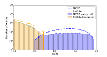
Figure 1: Distribution of events as a function of decl. for IceCube and HAWC. The figure shows the two datasets before and after applying energy and quality cuts. Restricting datasets to overlapping energy bins significantly reduces statistics for HAWC. The rates are dominated by events with energies near the threshold of each detector.
By imposing an artificial cut on low energies in the HAWC data, the detector response flattens since it becomes less dependent of zenith angle.
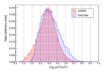
The statistics in HAWC with 300 tanks before cuts are comparable to one year of IceCube with 86 strings.Figure 2:
Energy distribution of the final event selection for the two datasets based on Monte Carlo simulations.
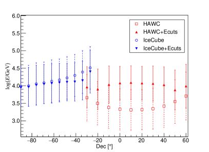
Figure 3: Median energy as a function of decl. for Monte Carlo simulations before and after applying energy cuts.
Figure 1 shows the distribution of data as a function of decl.
The resulting energy distribution of the two datasets is shown in Figure 2.
As a result of the applied energy cuts, both cosmic-ray data sets have a median primary particle energy of approximately 10 TeV with little dependence on zenith angle (Figure 3). The energy response of the observatories covers a 68% range of approximately 3 TeV - 40 TeV, in the case of IceCube, and 2.5 TeV - 30 TeV for HAWC around the median energy.
The two experiments have different response to the cosmic ray mass composition. This is largely due to the detection method.
Particles entering Earth’s atmosphere (15 to 20 km above sea level) interact with nuclei in air and produce a cascade of secondary particles. This particle cascade continues to grow until ionization becomes the dominant energy loss mechanism. The depth Xmax at which this happens depends on both the energy of the primary particle, and its mass. Lighter nuclei penetrate deeper than heavier nuclei. As a result, the altitude of extended air shower arrays such as HAWC
can affect the response of the detector to different nuclei since they are sensitive to the electromagnetic component of the particle shower. In contrast, the IceCube in-ice detector observes cosmic rays through the detection of deep penetrating muons produced from the decay of charged pions and kaons generated in the early interactions.
As a a result, for the same composition, IceCube’s response to different cosmic-ray nuclei differs from that of HAWC.
If the first interaction occurs at a lower air density (and higher elevation), mesons are more likely to decay to muons (and neutrinos) instead of re-interacting and producing lower energy pions and other secondary particles. As a result, the two experiments react differently to changes in atmospheric temperature and pressure.
IceCube (10 TeV)
HAWC (10 TeV)
Proton
0.756 0.018
0.6160 0.0054
He
0.195 0.009
0.3110 0.0014
CNO
0.028 0.004
0.0467 0.0004
NeMgSi
0.013 0.002
0.0191 0.0001
Fe
0.008 0.002
0.0078 0.0001
Table 2: Relative mass composition for 10 TeV median energy cosmic-rays in the two samples as determined from CORSIKA Monte Carlo simulations (Heck et al., 1998)
weighted to a Polygonato spectrum (Jörg R. Hörandel, 2003).
Errors reflect statistical uncertainties in the simulation datasets.
The data from both experiments are dominated by light nuclei (protons and alpha particles) as can be seen in Table 2.
All of the cuts applied were chosen based on CORSIKA Monte Carlo simulations (Heck et al., 1998) weighted to a Polygonato spectrum (Jörg R. Hörandel, 2003) and detailed simulations of the detector response.
5 Analysis
We compute the relative intensity as a function of J2000 equatorial
coordinates (, ) by binning the sky into an
equal-area grid with a bin size of using the
HEALPix library (Górski et al., 2005).
The angular distribution can be expressed as , where corresponds to the isotropic flux (i.e., the flux averaged over the full celestial sphere), and is the relative intensity of the flux as a function of R.A. and decl. in celestial coordinates.
Given that cosmic rays have been observed to be mainly isotropic, the flux is dominated by the isotropic term and therefore the anisotropy is small.
The relative intensity gives the amplitude of deviations in the number of counts from the isotropic
expectation in each angular bin . The residual anisotropy of the distribution of arrival directions of the cosmic rays is calculated by subtracting a reference map that describes the detector response to an isotropic flux
(2)
In order to produce this reference map, we must have a description of the arrival direction distribution if the cosmic rays arrived isotropically at Earth.
Ground-based experiments observe cosmic rays indirectly by detecting the secondary air shower particles produced by collisions of the cosmic-ray primary in the atmosphere.
The observed large-scale anisotropy has an amplitude of about but our simulations are not sufficiently accurate to describe the detector response at this level. We therefore calculate this expected flux from the data themselves in order to account for detector dependent rate variations in both time and viewing angle.
For Earth-based observatories, such a method requires averaging along each decl. band, thus washing out the vertical dependency (i.e. as a function of decl. ) in the relative intensity map .
A common approach is to estimate the relative intensity and detector exposure simultaneously using time-integration methods (Alexandreas et al., 1993; Atkins et al., 2003).
However, these methods can lead to an under- or overestimation of the isotropic reference level
for detectors located at mid latitudes, since a fixed position on the celestial sphere is only observable over a relatively short period every day.
As a result, the total number of cosmic ray events from this fixed position can only be compared against reference data observed during the same period.
Therefore, time-integration methods can strongly attenuate large-scale structures exceeding the size of the instantaneous field of view (Ahlers et al., 2016).
5.1 Maximum Likelihood Method
For this analysis, we have relied on the likelihood-based reconstruction described in Ahlers et al. (2016) and recently applied in the study of the large-scale cosmic-ray anisotropy by HAWC (Abeysekara et al., 2018b).
The method does not rely on detector simulations and provides an optimal anisotropy reconstruction and the recovery of the large-scale anisotropy projected on to the equatorial plane for ground-based cosmic ray observatories located in the middle latitudes as HAWC.
The generalization of the maximum likelihood method for combined data sets from multiple observatories that have exposure to overlapping regions of the sky is described in Appendix A.
5.2 Statistical Significance
In order to calculate the statistical significance of anisotropy features in the final reconstructed map, Ahlers et al. (2016) generalizes the method in Li & Ma (1983) to account for the optimization process of the time-dependent exposure.
The significance map (in units of Gaussian ) is then calculated as
(3)
For each pixel
in the celestial sky, we define expected on-source and off-source event counts from neighbor pixels in a disc of radius centered on that pixel. For this analysis we have chosen a radius of 5∘. Given the set of pixels , the observed and expected counts are
(4)
(5)
(6)
where is the relative acceptance of the detector in pixel and sidereal time bin , gives the expected number of isotropic events in sidereal time bin , is the relative intensity, and where is divided into a contribution from the reference map and the residual relative intensity.
For small-scale features, corresponds to the first 3 spherical harmonic components () of the relative intensity.
In order to distinguish excess and deficit, we multiply Eq. 3 by the sign of each smoothed pixel in the anisotropy map.
5.3 Harmonic Analysis and Dipole Fit
The relative intensity can be decomposed as a sum over spherical harmonics ,
(7)
The vector components of the dipole in terms of the spherical harmonic expansion in equatorial coordinates are related to the
coefficients with
(8)
where and are respectively, the real and imaginary components of , and taking into account that and (see Ahlers & Mertsch (2017)).
From equation 8 and the coefficients,
one can obtain the horizontal components of the dipole
and with respect to the h and h R.A. axes.
The phase and
amplitude of the projected dipole on the equatorial plane are given by
(9)
where
is the phase and is the amplitude of the projected dipole on the equatorial plane and it is related to the true amplitude through the dipole inclination with .
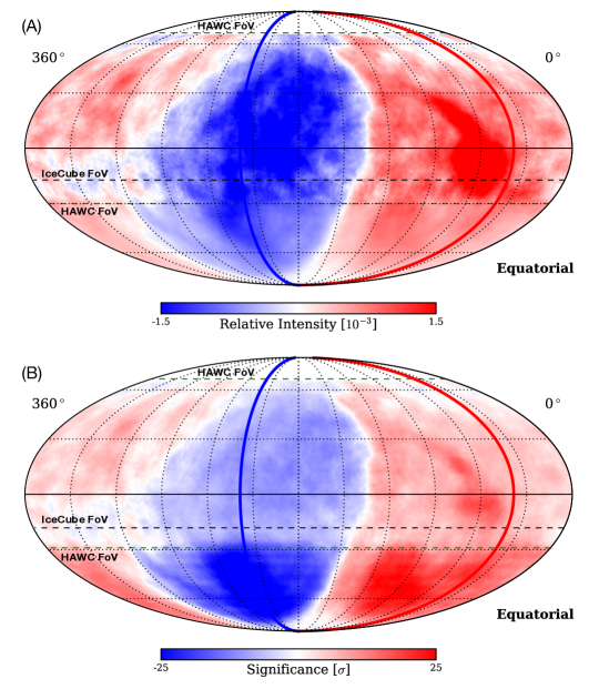
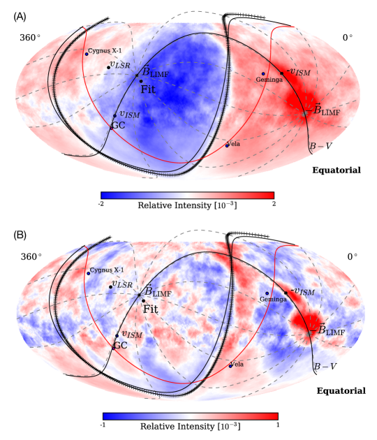
Figure 4: Mollweide projection sky maps of (A) relative intensity (Eq. 2) of cosmic-rays at 10 TeV median energy
and (B) corresponding
signed statistical significance (Eq. 3) of the deviation from the average intensity in J2000 equatorial coordinates.
The thick red and blue lines in the figures indicate correspondingly, the node and antinode of the phase in R.A. of the dipole component from the fit.
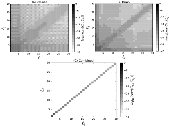
5.4 Angular Power Spectrum
The angular power spectrum for the relative intensity field is defined as:
(10)
for each value of .
Since this analysis is not sensitive to the vertical component of the anisotropy, the largest recoverable dipole amplitude has the terms missing and we can only measure a pseudo power spectrum :
(11)
The angular power spectrum provides an estimate of the significance of structures at different angular scales of 180.
In the ideal case of a sky coverage, the multipole moments of the reconstructed anisotropy would carry all the information of the anisotropy (except for the vertical component terms). However, as will be discussed in Section 7.2, partial sky coverage of individual experiments further limits the amount of information that can be obtained from the reconstructed pseudo multipole moment spectrum.
6 Results
The measured relative intensity map is shown in Figure 4.
A smoothing procedure was applied to all maps using a top-hat function in which a single pixel’s value is the average of all pixels within a 5∘ radius.
The map shows an anisotropy in the distribution of arrival directions of
cosmic rays with 10 TeV median primary particle energy that extends across both hemispheres.
The significance (smoothed by summing over pixels) of the IceCube region reflects the much larger statistics in the IceCube dataset compared to that from HAWC at energies of 10 TeV.
Figure 5: (A) Relative intensity (Eq. 2)
after subtracting the multipole fit from the large-scale map and (B) corresponding
signed statistical significance (Eq. 3) of the deviation from the average intensity in J2000 equatorial coordinates.
Figure 5 is the residual small-scale anisotropy after subtracting the fitted multipole from the spherical harmonic expansion
with
from the large-scale map in Figure 4 in order to reveal structures smaller than .
The large-scale structure and significant small-scale structures in Figures 4 and 5 are largely consistent with previous individual measurements, as shown in Figure 6.
Observed features extend across the horizon of both datasets. The one referred to as “region A” by the Milagro Collaboration (Abdo et al., 2008) roughly extends from , to , in equatorial coordinates (, ). The so called “region B” (Abdo et al., 2008) corresponds to the boundary between the excess and deficit regions (see Figure 4) in the northern sky that appears as a small scale feature (see Figure 5) for short integration times.
Table 3: Spherical Harmonic Coefficients []
1
2
3
4
5
6
7
1
-13.26 +10.49
2
-0.21 -3.6
-7.20 +2.05
3
1.75 -1.7
-2.03 +0.13
0.20 +0.17
4
1.70 -0.52
0.07 +1.69
-0.86 -0.8
-1.19 +0.04
5
0.58 +0.27
-0.07 -1.1
-1.64 -0.051
0.18 -0.15
-0.11 -1.5
6
0.80 -0.88
-0.24 -0.38
-0.10 +0.63
0.13 -1.2
0.27 +0.47
1.65 -0.53
7
0.44 -0.67
0.37 +0.15
-0.21 -0.14
-0.70 +0.04
0.84 -0.27
0.13 -0.54
0.07 +0.91
8
0.26 +0.06
0.14 -0.47
-0.39 -0.22
-0.42 +0.72
-0.15 -0.15
-0.72 -0.61
0.42 +0.36
9
0.11 -0.88
-0.29 -1.3
0.22 -0.17
0.12 -0.56
-0.01 -0.34
0.60 +0.47
-0.06 -0.48
10
0.21 -0.97
0.25 -0.5
0.21 -0.65
0.09 -0.088
-0.10 +0.12
0.11 -0.017
0.02 +0.19
11
0.56 -0.39
0.06 -0.42
-0.15 -0.68
-0.04 +0.05
-0.26 +0.04
-0.07 -0.26
-0.16 +0.25
12
0.40 +0.07
0.19 -0.56
-0.27 -0.48
-0.17 -0.1
-0.13 -0.18
-0.03 -0.23
0.33 +0.13
13
0.45 -0.33
-0.04 -0.69
0.17 -0.92
-0.26 -0.6
0.13 +0.24
-0.08 +0.02
0.04 +0.04
14
0.57 -0.16
0.13 -0.53
0.17 -1.1
-0.31 -0.089
0.08 -0.09
-0.25 -0.12
-0.05 +0.22
8
9
10
11
12
13
14
8
-0.54 +0.19
9
0.15 +0.64
-0.04 +0.45
10
0.22 +0.12
-0.66 -0.57
-0.26 +0.38
11
0.25 +0.02
-0.21 -0.4
0.15 -0.25
-0.06 -0.18
12
0.37 +0.09
-0.46 +0.25
-0.13 +0.20
-0.08 +0.21
0.04 -0.18
13
0.11 +0.13
0.13 -0.13
-0.35 -0.098
0.39 +0.45
-0.01 -0.3
0.41 -0.17
14
-0.13 +0.34
0.36 -0.11
-0.04 -0.072
-0.11 -0.17
-0.19 +0.32
0.13 +0.21
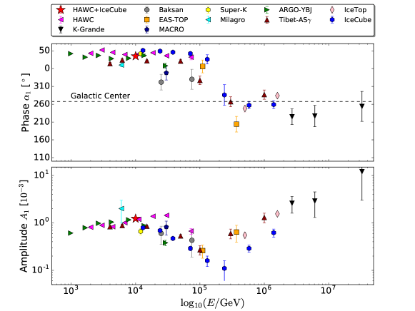
0.18 +0.35
Figure 6: Reconstructed dipole component amplitude and phase from this measurement along previously published TeV-PeV results from other experiments (adopted from Ahlers & Mertsch (2017)). The results shown are from Abeysekara et al. (2018b); Chiavassa et al. (2015); Alekseenko et al. (2009); Aglietta et al. (2009); Ambrosio et al. (2003); Guillian et al. (2007); Abdo et al. (2009); Bartoli et al. (2015); Amenomori et al. (2005); Aartsen et al. (2013, 2016)
We obtain the through a transformation of spherical harmonics using the HEALPix function map2alm. The results are presented in Table 3.
The horizontal components of the dipole obtained from equation
(8) using the values in Table 3 are
and
, respectively, with respect to the h and h R.A. axes.
The dipole amplitude and phase
,
measured in this combined study are shown in Figure 6 along with
previously published results from other experiments in the TeV-PeV primary particle energy range. The combined systematic uncertainty in the amplitude and phase of the dipole are expected to be , and respectively (see section 7).
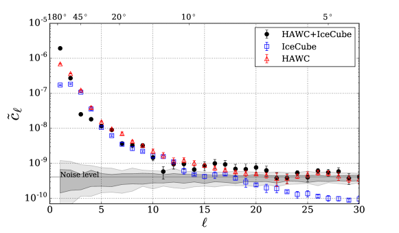
Figure 7: Angular power spectrum of the cosmic ray anisotropy at 10 TeV.
The gray band represents the 90% confidence level around the level of statistical fluctuations for isotropic sky maps.
The noise level is dominated by limited statistics for the portion of the sky observed by HAWC. The IceCube dataset alone has a lower noise level and is sensitive to higher components.
The dark and light gray bands represent the power spectra for isotropic sky maps at the 68% and 95% confidence levels respectively.
The errors do not include systematic uncertainties from partial sky coverage.
The angular power spectrum for the combined dataset in Figure 7 provides an estimate of the significance of structures at different angular scales of 180. Biases are substantially reduced with the likelihood method and by eliminating degeneracy between multipole moments with a nearly full sky coverage. The angular power spectrum can therefore be considered to be the physics fingerprint of the observed 10 TeV anisotropy, providing information about the propagation of cosmic rays and the turbulent nature of the Local Interstellar Magnetic Field (LIMF) (Giacinti & Sigl, 2012; Ahlers & Mertsch, 2017). The large discrepancy between the combined and individual datasets is the result of the limited sky coverage by each experiment. This systematic effect will be discussed in Section 7.2.
A residual limitation in this analysis is the fact that ground-based experiments are generally not sensitive to the vertical component of the anisotropy as discussed by Abeysekara et al. (2018b) and Ahlers et al. (2016), as mentioned earlier.
The measured quadrupole component has an amplitude of and is inclined at above (and below) equatorial plane.
As with the dipole, the fitted quadrupole component from the spherical harmonic expansion is also missing the terms. However, the combination of and non-vertical quadrupole components can still provide valuable information.
The experimental determination of the vertical components of the anisotropy would require accuracies better than the amplitude of the anisotropy ().
This becomes easier at ultra-high energies where a dipole of much larger amplitude has been observed (Aab et al., 2017).
The full-sky coverage also provides better constraints for fitting the and multipole components and reduces correlations between spherical harmonic expansion coefficients .
7 Systematics Studies
7.1 Overlapping Region
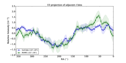
Figure 8: One-dimensional R.A. projection of the relative intensity of cosmic rays
for adjacent bins in the overlap region at -20∘
for HAWC and IceCube data.
There is general agreement for large scale structures.
The two curves correspond to different bands. The shaded bands correspond to systematic uncertainties due to mis-reconstructed events,
derived from the relative intensity distributions in adjacent decl. bands between and .
We have studied two adjacent bands at -20∘ for HAWC and IceCube data near the horizon of each detector (see Figure 8). The HAWC band extends from -21∘ to -19∘ while the IceCube band extends from -22∘ to -20∘.
The large structure between the two datasets is consistent though small structures differ.
It is worth noting that the overlap region is where we expect to find the largest difference in median energy between the two datasets (see Figure 3).
The angular resolution of both detectors also decreases toward the horizon. While HAWC data has a smaller point spread function at this decl. and is sensitive to structures on smaller scales, IceCube has better statistics so the structures are more significant.
One particular feature that stands out is the excess in HAWC around that coincides with the so called “region A”.
There appears to be a corresponding small excess in the IceCube data.
It is also worth noting that statistics in this region are quickly decreasing with increasing zenith angle as is the quality of angular reconstructions. As a result, bins closer to the horizon contain a high level of contamination from bins in higher zenith angles.
7.2 Partial Sky Coverage
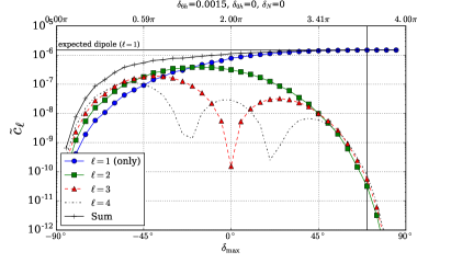
Figure 9:
Angular power spectrum as a function of sky coverage for . The horizontal axis indicates the maximum decl. , keeping for a dipole injected horizontally in direction . The partial coverage of sky produces an artificial quadrupole and octupole that decrease in power with greater celestial coverage.
Incomplete coverage of the sky leads to an underestimation of the angular power of the dipole perpendicular to the axis of rotation of the Earth.
The pseudo-moments of the projected dipole, and , are corrected by a geometric factor introduced by Ahlers et al. (2016)
in order to estimate the true moments and .
Furthermore, there is a degeneracy between different pseudo-modes under partial sky coverage that primarily affects the multipolar components , , and to a lesser degree, as has been previously studied by Sommers (2001).
This effect is evident in Figure 9 which corresponds to a dipole injected horizontally in the direction . The partial coverage of the sky produces an artificial quadrupole, octupole and hexadecapole that, in the case of a horizontal dipole, decrease in power with greater celestial coverage. The horizontal axis indicates the maximum observable decl. , keeping .
Figure 10: Correlation matrix for modes with partial sky coverage from individual experiments (A, B) and for the combined field of view (C).
From Figure 9 it is possible to see that the spurious quadrupole and octupole components (which are significant for partial integrated sky coverage) are reduced to an amplitude to order in this analysis.
Figure 10 shows the correlation matrix (Efstathiou, 2004) of the different -modes up to calculated using the PolSpice111
PolSpice website: http://www2.iap.fr/users/hivon/software/PolSpice/. software package. The correlation between -modes due to partial sky coverage is appreciable for larger , though to a lesser degree.
7.3 Seasonal Variations and Local Variations in Solar Time
The relative motion of the Earth around the Sun can introduce a systematic solar dipole, a dipole anisotropy analogous to the Compton-Getting effect (Compton & Getting, 1935) produced by the motion of Earth around the Sun, that points in the direction of Earth’s orbital velocity vector.
The influence of diurnal variations (such as the solar dipole) on the sidereal anisotropy can be estimated from the influence it has on the anti-sidereal distribution in a frame with 364.24 cycles per year (see, e.g. Guillian et al. (2007)). Any significant variations in this frame result from a modulation of the solar frame and represents a systematic effect of the solar frame on the sidereal anisotropy (Aartsen et al., 2016). The anti-sidereal distribution of the HAWC dataset has a maximum amplitude of . Both contamination from the solar dipole and atmospheric pressure variations are included in this systematic.
For IceCube, the same systematic uncertainty is at the level of . The worst-case uncertainty on the reconstructed phase of the dipole is and a combined systematic uncertainty of for the dipole amplitude.
The solar dipole anisotropy produced by the motion of Earth around the Sun is given by the equation
(12)
where is the cosmic-ray intensity, is the index of the differential energy spectrum of cosmic rays, is the velocity of the Earth, is the speed of light
and is the angle between the direction of the reconstructed cosmic rays and the direction of the velocity vector (Compton & Getting, 1935).
This vector rotates by such that, after one year, the effect is ideally completely cancelled for 100% duty cycle of observation. However, a residual dipole can be introduced if the data does not cover an integer number of years with uniform coverage.
In other words, any gaps in data taking can result in a slight bias to the measured dipole. A solar dipole anisotropy at the level of has been previously observed at
several TeVs (Amenomori et al., 2004, 2006; Abdo et al., 2009; Abbasi et al., 2011, 2012; Bartoli et al., 2015). Based on Monte Carlo studies, the residual contribution solar dipole that results from gaps in data taking is estimated to be of order for the HAWC dataset, which is smaller than the statistical error of this analysis. In the case of IceCube, the detector has an uptime of 99% (see Aartsen et al. (2017)) reduced to an uptime of 95.4% after selecting full sidereal days. As a result, the systematic effect of data gaps is smaller (Abbasi et al., 2012).
In addition to variations caused by the anisotropy and the solar dipole, there may also be local variations in the detection of cosmic rays caused by changes in atmospheric conditions, such as pressure and temperature, and also by changes in the detector.
For 10 TeV energies, HAWC is located below the shower maximum Xmax for all primary masses. As a result, an increase in pressure leads to an increase of the atmospheric overburden which results in an attenuation of shower sizes. Atmospheric overburden is related to ground pressure as , where 9.87 m s-2 is the local gravitational acceleration (Abbasi et al., 2013).
In first order approximation, the simple correlation
between the change in the logarithm of the rate and the surface
pressure change is
(13)
where is the barometric coefficient (Tilav et al., 2010).
The variations in atmospheric pressure at the HAWC site are primarily due to atmospheric tides driven by temperature and a small contribution from gravitational tides (Zhang et al., 2010).
We have studied the effect of atmospheric pressure variations by applying a correction to the data rate to account for measured changes in pressure at the HAWC site. The procedure involves determining the correlation coefficient between the surface pressure data and the detector rate from Eq. 13 in order to weight individual events. This yields a barometric coefficient of hPa-1 The residual contamination from atmospheric variations is estimated to be on the order of . Temperature variations in the stratosphere can introduce a similar effect with a 24h cycle and a 365 day cycle. However, this effect is small for latitudes near the equator and in the case of the daily variations, it is a smaller effect than that of pressure variations.
In contrast with HAWC, where the event rate is anti-correlated with atmospheric pressure and with the effective temperature of the stratosphere, the muon rate in IceCube is directly correlated with the effective temperature (Tilav et al., 2010).
Event rate variations in IceCube have an annual period since one day at the South Pole lasts 365 days instead of 24 hours. In the case of IceCube there are also faster atmospheric variations of lower amplitude but these approximately affect the event rate globally in all azimuth directions (with a maximum Kolmogorov-Smirnov distance below for daily variations at a 90% confidence level). Due to the geometry of the detector and its location at the South Pole, this also means that such variations equally affect every angle in R.A.
Seasonal variations in the effective temperature can introduce modulations in the intensity of the Solar dipole. As a result, the Solar dipole would not average to zero over a full year and thus would produce a residual bias. However, the amplitude of the anti-sidereal distribution indicates that this is not a significant effect.
8 Discussion
The combined sky map of arrival direction distribution of the 10 TeV cosmic rays collected by HAWC and IceCube and the corresponding power spectrum of its spherical harmonics components, may provide important hints on the origin of the observation. In particular, the angular power spectrum can reveal information about how cosmic rays propagate through the interstellar medium while the large-scale arrival direction distribution provides hints about the structure of the nearby LIMF and the heliosphere.
Figure 11: (A) Relative intensity of cosmic-rays at 10 TeV median energy (Figure 4(A)) and (B) corresponding small-scale anisotropy (Figure 5(A)) in J2000 equatorial coordinates with color scale adjusted to emphasize features. The fit to the boundary between large scale excess and deficit regions is shown as a black crossed curve. The magnetic equator from Zirnstein et al. (2016) is shown as a black curve as is the plane containing the local interstellar medium magnetic field and velocity ( plane). The Galactic plane is shown as a red curve and two nearby supernova remnants, Geminga and Vela are shown for reference as is Cygnus X-1, a black hole X-ray binary known to produce high energy
rays (Albert et al., 2007).
8.1 Cosmic Ray Propagation in the Interstellar Medium
The angular power spectrum in Figure 7 shows two different regimes: a steeply falling slope at large scales and a softer slope at small scales . This suggests that two different mechanisms are responsible for the structures observed in the sky map.
The steep portion of the angular power spectrum may be associated with large scale diffusive processes (over many mean free paths) across the interstellar medium, as suggested by Erlykin & Wolfendale (2006); Blasi & Amato (2012); Ptuskin (2012); Pohl & Eichler (2013b); Sveshnikova et al. (2013); Savchenko et al. (2015); Ahlers (2016); Giacinti & Kirk (2017).
On the other hand, the softer slope portion appears to be consistent with non-diffusive pitch angle scattering effects on magnetic turbulence within the mean free path (Giacinti & Sigl, 2012) and with that obtained from numerical calculations of sub-PeV protons propagating through incompressible magnetohydrodynamic turbulence (López-Barquero et al., 2016).
In Ahlers (2014) it is shown that under certain conditions, those small-scale structures arise as natural consequence of hierarchical evolution of angular scales under Liouville’s theorem.
The dipole component of the anisotropy may provide a hint into the direction of the large scale cosmic ray density gradient on the equatorial plane, thus linking the observed anisotropy with possible contributions of the closest sources, such as the Vela supernova remnant at a distance of about 0.3 kpc and with an age of about
11 kyr (Ahlers & Mertsch, 2017). The fact that Vela is located within the large-scale excess region of the sky is consistent with it being a potential source contributing to the large-scale anisotropy.
However, predictions of the anisotropy amplitude depend on many unknown factors such as the actual contributing source (or sources), the diffusion coefficient, and the unknown component of the anisotropy perpendicular to the equatorial plane that complicate such calculations.
The measured amplitude and phase in this study is consistent with
observations from multiple experiments that show a turning point in the energy dependency of the dipole component amplitude at an energy scale of 10 TeV (see Figure 6). After initially increasing with energy, the dipole amplitude begins to decrease above 10 TeV, while the phase has an abrupt change at the 100 TeV energy scale where the amplitude begins to increase again. Cosmic rays with rigidity of 10 TV have a gyro-radius of about 700 AU in a 3 G magnetic field, which is comparable to the transversal size of the heliosphere (i. e. perpendicular to the long axis) (Pogorelov et al., 2009, 2013; Pogorelov, 2016). It is reasonable to assume that at lower energies the heliospheric influence is important, while above 10 TV the interstellar influence is progressively more important (Desiati & Lazarian, 2013).
An understanding of how interstellar propagation of 10 TV-scale cosmic rays influences the arrival direction distribution must, therefore, also take into account heliospheric effects (Schwadron et al., 2014; López-Barquero et al., 2017; Zhang & Pogorelov, 2016). An alternative approach is to study cosmic ray anisotropy above 100 TV rigidity (Aartsen et al., 2013, 2016), where the heliospheric influence is expected to be negligible. In this case, the arrival direction distribution can be used to probe the global properties of interstellar turbulence by fitting theoretical models to observations (Giacinti & Kirk, 2017). However, at high energies a full-sky study is currently not possible with the dataset used in this analysis due to limited statistics.
8.2 Large-scale Anisotropy and the Local Interstellar Magnetic Field
Figure 12: distribution map for circular fit to boundary between large-scale excess and deficit regions shown in J2000 equatorial coordinates. The black point corresponds to the minimum for the center of the circle and the black curve is the fitted circle. The grey points are the selected pixels for the fit. The best fit has a value of /ndof .
Figure 13: Circular fit to boundary between large-scale excess and deficit regions shown in J2000 equatorial coordinates along with published magnetic field measurements by Funsten et al. (2013)
inferred from the emission of energetic neutral atoms (ENA) originating from the outer heliosphere by the Interstellar Boundary Explorer (IBEX) (Zirnstein et al., 2016), and
Frisch et al. (2015) obtained from the polarization of stars within 40 pc.
Figure 11 shows the direction of the LIMF from Zirnstein et al. (2016) and the corresponding equator (the continuous black line), the so-called plane defined by the LIMF and the direction of the Sun’s velocity through the interstellar medium , as well as the direction of the velocity relative to the local standard of rest . The figure also shows the location of the Geminga and Vela supernova remnants as possible contributing sources, and those of the Cygnus X-1 X-ray binary and Galactic center GC for reference. The location of the Galactic plane is shown as a red line.
A fit to the plane defined by the small-scale feature that marks the boundary between the excess and deficit regions ( R.A.) is shown in Figure 12. The fit yields a vector pointed towards
in J2000 equatorial coordinates, as shown in Figure 11, along with the corresponding equator (the crossed black curve).
The direction is located from the LIMF inferred by the Interstellar Boundary Explorer (IBEX) from the emission of energetic neutral atoms (ENA) originating from the outer heliosphere (see Funsten et al. (2013). This point is also located from the LIMF direction
reported by Zirnstein et al. (2016)
and consistent with the average LIMF direction
obtained from the polarization of stars within 40 pc by Frisch et al. (2015).
This is shown in Figure 13 and summarized in Table 4 along with the value of obtained from the dipole fit and the value of obtained from the quadrupole fit. The errors on the fit are derived from the distribution shown in Figure 12 and don’t include possible systematics uncertainties from the missing dipole component.
Table 4: Magnetic field alignment. The last two rows correspond to measurements of the large-scale anisotropy from this study. The R.A. measurement in the last row is obtained from the dipole vector and the decl. is obtained from the quadrupole component. The second to last column corresponds to the angular distance between the boundary fit and the various LIMF estimates.
The last column gives the corresponding vertical dipole component under the assumption that the dipole is oriented towards the given decl. Error in parentheses for dipole and quadruple correspond to systematic uncertainties.
The fact that the dipole component of the full-sky cosmic ray anisotropy map is approximately aligned with the direction of the LIMF (or at least its projection on the equatorial plane) is probably not a coincidence, since we expect diffusion to be anisotropic with the fastest propagation along the magnetic field lines (Effenberger, F. et al., 2012; Kumar & Eichler, 2014b; Schwadron et al., 2014; Mertsch & Funk, 2015).
Assuming that the observed dipole points in this direction, it is possible to estimate the amplitude of the vertical component. The measured amplitude of the horizontal component of the dipole is related to the true amplitude through the dipole inclination with , from which we obtain a value for the vertical dipole vector component of
for the various magnetic field assumptions (see Table 4).
If we assume that the dipole component must be aligned with the LIMF, the observed
deviation could be explained as due to the relative motion of the observer with respect to a frame in which the cosmic ray distribution is isotropic, called the Compton-Getting Effect (Compton & Getting, 1935; Gleeson & Axford, 1968).
The heliosphere could also have a significant warping effect on 10 TeV cosmic ray arrival direction distribution, mostly due to the LIMF draping curvature around the heliosphere (Pogorelov et al., 2009).
As a result, the dipole component of the cosmic ray anisotropy could be out of alignment from the LIMF.
Future studies, with full-sky maps at different particle rigidities, could provide a more powerful tool to probe the properties of the interstellar
and heliospheric magnetic fields.
9 Conclusions
We have used experimental data collected by the HAWC Gamma Ray Observatory and the IceCube Neutrino Observatory to compile, for the first time, a nearly full-sky map of the arrival direction distribution of cosmic rays with median energy of 10 TeV.
The combined analysis accounts for the difference in instantaneous and time-integrated field of view of the HAWC observatory and provides an integrated field of view that extends from to in decl. The almost full-sky observation eliminates the degeneracy between the spherical harmonic components and provides a tool to probe the properties of particle diffusion in the interstellar medium and of interstellar magnetic turbulence.
The corresponding angular power spectrum suggests that two different mechanisms are responsible for the observed angular scale features. The ordering of cosmic ray anisotropy along the LIMF is supported by fitting the boundary between deficit and excess, which points to the direction that is consistent with various observations. We obtained the phase and amplitude of the dipole component projected onto the equatorial plane to be ,
. Based on the assumption that the true dipole is aligned along the LIMF, we estimated the missing vertical component to be .
Acknowledgements
Dedicated to the memory of our honorable colleague,
and dear friend Stefan Westerhoff.
The IceCube collaboration acknowledges the significant contributions to this manuscript from M. Ahlers, P. Desiati., and J. C. Díaz-Vélez. The HAWC Collaboration acknowledges additional contributions from D. W. Fiorino.
The HAWC Collaboration acknowledges the support from: the US National Science Foundation (NSF) the US Department of Energy Office of High-Energy Physics;
the Laboratory Directed Research and Development (LDRD) program of Los Alamos National Laboratory;
Consejo Nacional de Ciencia y Tecnología (CONACyT), México (grants 271051, 232656, 260378, 179588, 239762, 254964, 271737, 258865, 243290, 132197, 281653)(Cátedras 873, 1563, 341), Laboratorio Nacional HAWC de rayos gamma;
L’OREAL Fellowship for Women in Science 2014;
Red HAWC, México;
DGAPA-UNAM (grants IG100317, IN111315, IN111716-3, IA102715, IN109916, IA102917, IN112218);
VIEP-BUAP;
PIFI 2012, 2013, PROFOCIE 2014, 2015;
the University of Wisconsin Alumni Research Foundation;
the Institute of Geophysics, Planetary Physics, and Signatures at Los Alamos National Laboratory;
Polish Science Centre grant DEC-2014/13/B/ST9/945, DEC-2017/27/B/ST9/02272;
Coordinación de la Investigación Científica de la Universidad Michoacana; Royal Society - Newton Advanced Fellowship 180385. Thanks to Scott Delay, Luciano Díaz and Eduardo Murrieta for technical support.
The IceCube Collaboration acknowledges the support from:
USA – U.S. National Science Foundation-Office of Polar Programs,
U.S. National Science Foundation-Physics Division,
Wisconsin Alumni Research Foundation,
Center for High Throughput Computing (CHTC) at the University of Wisconsin-Madison,
Open Science Grid (OSG),
Extreme Science and Engineering Discovery Environment (XSEDE),
U.S. Department of Energy-National Energy Research Scientific Computing Center,
Particle astrophysics research computing center at the University of Maryland,
Institute for Cyber-Enabled Research at Michigan State University,
and Astroparticle physics computational facility at Marquette University;
Belgium – Funds for Scientific Research (FRS-FNRS and FWO),
FWO Odysseus and Big Science programmes,
and Belgian Federal Science Policy Office (Belspo);
Germany – Bundesministerium für Bildung und Forschung (BMBF),
Deutsche Forschungsgemeinschaft (DFG),
Helmholtz Alliance for Astroparticle Physics (HAP),
Initiative and Networking Fund of the Helmholtz Association,
Deutsches Elektronen Synchrotron (DESY),
and High Performance Computing cluster of the RWTH Aachen;
Sweden – Swedish Research Council,
Swedish Polar Research Secretariat,
Swedish National Infrastructure for Computing (SNIC),
and Knut and Alice Wallenberg Foundation;
Australia – Australian Research Council;
Canada – Natural Sciences and Engineering Research Council of Canada,
Calcul Québec, Compute Ontario, Canada Foundation for Innovation, WestGrid, and Compute Canada;
Denmark – Villum Fonden, Danish National Research Foundation (DNRF), Carlsberg Foundation;
New Zealand – Marsden Fund;
Japan – Japan Society for Promotion of Science (JSPS)
and Institute for Global Prominent Research (IGPR) of Chiba University;
Korea – National Research Foundation of Korea (NRF);
Switzerland – Swiss National Science Foundation (SNSF).
Appendix A Generalized Maximum likelihood method for multiple observatories with overlapping fields of view
The method developed by Ahlers et al. (2016) assumes that the detector exposure per solid angle and sidereal time accumulated over many sidereal days can be expressed as a product of its angular-integrated exposure per sidereal time and relative acceptance (normalized as ):
(A1)
with the assumption that the relative acceptance of the detector does not strongly depend on sidereal time.
For each observatory, the number of cosmic rays expected from
an angular element of the local coordinate sphere corresponding to coordinates in a sidereal time interval is
(A2)
where gives the expected number of isotropic events in sidereal time bin independent of pixel,
is the relative acceptance of the detector for pixel , and
is the relative intensity observed in local coordinates during time bin . is the time-dependent coordinate transformation of the unit vector that corresponds to the coordinates in the right-handed equatorial system.
Here, we adopt the convention used by Ahlers et al. (2016) where roman indices (, ) refer to pixels in the local sky map
and fraktur indices () refer to pixels in the celestial sky map
while time bins are indicated by greek indices (, ).
The data observed at a fixed sidereal time bin
can be described in terms of the observation in local horizontal sky with bin as or transformed into the celestial sky map with bin as .
The likelihood of observing cosmic rays is then given by the product of Poisson probabilities
(A3)
where .
We maximize the likelihood ratio
of signal over null hypothesis of no anisotropy (, , ),
(A4)
with . The maximum likelihood estimators of and are then
(A5)
(A6)
given the boundary condition
(A7)
In this combined analysis of HAWC and IceCube data, the likelihood (Eq. A3) is generalized to a product over data sets with individual detector exposures
but the same relative intensity.
The total accumulated exposure in Eq. (A1) becomes a sum over disjoint sky sectors, whose union covers the entire field of view. In this analysis the integrated field of view of each detector corresponds to a sector. As before, we assume that the exposure in each sector can be expressed as a product of its angular-integrated exposure and relative acceptance in terms of azimuth and zenith angle as
(A8)
The values of , , and of the maximum likelihood ratio (Eq. A4) must obey the implicit relations
(A9)
(A10)
(A11)
Here, we have introduced the window function of the sector which is equal to if the pixel is located in the sector and otherwise.
The binned quantity
in Eq. (A9), corresponds to the relative acceptance of sector seen in the equatorial coordinate system in pixel during time bin .
Equations (A9) to (A11) correspond to a nonlinear set of equations that cannot be solved in explicit form
but one can iteratively approach the best-fit solution.
This reconstruction method is a simple generalization of the iterative method outlined in
Ahlers et al. (2016), where now the relative acceptances and isotropic expectation for each detector are evaluated as independent quantities. This is a valid approach as long as the rigidity distributions of the data sets are very similar.
References
Aab et al. (2017)
Aab, A., Abreu, P., Aglietta, M., et al. 2017, Science, 357, 1266
Aartsen et al. (2017)
Aartsen, M., Ackermann, M., Adams, J., et al. 2017, J. Inst., 12, P03012
Aartsen et al. (2013)
Aartsen, M. G., Abbasi, R., Abdou, Y., et al. 2013, ApJ, 765, 55
Aartsen et al. (2016)
Aartsen, M. G., Abraham, K., Ackermann, M., et al. 2016, ApJ, 826, 220
Abbasi et al. (2010)
Abbasi, R., Abdou, Y., Abu-Zayyad, T., et al. 2010, ApJ, 718, L194
Abbasi et al. (2011)
—. 2011, ApJ, 740, 16
Abbasi et al. (2012)
—. 2012, ApJ, 746, 33
Abbasi et al. (2013)
—. 2013, Astropart. Phys., 44, 40
Abdo et al. (2008)
Abdo, A. A., Allen, B., Aune, T., et al. 2008, Phys. Rev. Lett., 101, 221101
Abdo et al. (2009)
Abdo, A. A., Allen, B. T., Aune, T., et al. 2009, ApJ, 698, 2121
Abeysekara et al. (2018a)
Abeysekara, A., Alfaro, R., Alvarez, C., et al. 2018a, NIM Phys.
Res. A, 888, 138
Abeysekara et al. (2014)
Abeysekara, A. U., Alfaro, R., Alvarez, C., et al. 2014, ApJ, 796, 108
Abeysekara et al. (2017)
Abeysekara, A. U., Albert, A., Alfaro, R., et al. 2017, ApJ, 843, 39
Abeysekara et al. (2018b)
Abeysekara, A. U., Alfaro, R., Alvarez, C., et al. 2018b, ApJ,
865, 57
Aglietta et al. (2009)
Aglietta, M., Alekseenko, V. V., Alessandro, B., et al. 2009, ApJ, 692, L130
Ahlers (2014)
Ahlers, M. 2014, Phys. Rev. Lett., 112, 021101
Gleeson & Axford (1968)
Gleeson, L. J., & Axford, W. I. 1968, Astrophys. & Sp. Sci., 2, 431
Górski et al. (2005)
Górski, K. M., Hivon, E., Banday, A. J., et al. 2005, ApJ, 622, 759
Guillian et al. (2007)
Guillian, G., Hosaka, J., Ishihara, K., et al. 2007, Phys. Rev. D, 75, 062003
Hall et al. (1999)
Hall, D. L., Munakata, K., Yasue, S., et al. 1999, J. Geophys. Res., 104, 6737
Heck et al. (1998)
Heck, D., Knapp, J., Capdevielle, J., Schatz, G., & Thouw, T. 1998, CORSIKA: A
Monte Carlo code to simulate extensive air showers, 51.02.03; LK 01;
Wissenschaftliche Berichte, FZKA-6019 (Februar 98)
Hunter (2007)
Hunter, J. D. 2007, Computing In Science & Engineering, 9, 90
Jörg R. Hörandel (2003)
Jörg R. Hörandel. 2003, Astropart. Phys., 19, 193
Kumar & Eichler (2014a)
Kumar, R., & Eichler, D. 2014a, ApJ, 785, 129
Kumar & Eichler (2014b)
—. 2014b, ApJ, 785, 129
Li & Ma (1983)
Li, T. P., & Ma, Y. Q. 1983, ApJ, 272, 317
López-Barquero et al. (2016)
López-Barquero, V., Farber, R., Xu, S., Desiati, P., & Lazarian, A.
2016, ApJ, 830, 19
López-Barquero et al. (2017)
López-Barquero, V., Xu, S., Desiati, P., et al. 2017, ApJ, 842, 54