Split Regression Modeling

Abstract

Sparse methods are the standard approach to obtain interpretable models with high prediction accuracy. Alternatively, algorithmic ensemble methods can achieve higher prediction accuracy at the cost of loss of interpretability. However, the use of blackbox methods has been heavily criticized for high-stakes decisions and it has been argued that there does not have to be a trade-off between accuracy and interpretability. To combine high accuracy with interpretability, we generalize best subset selection to best split selection. Best split selection constructs a small number of sparse models learned jointly from the data which are then combined in an ensemble. Best split selection determines the models by splitting the available predictor variables among the different models when fitting the data. The proposed methodology results in an ensemble of sparse and diverse models that each provide a possible explanation for the relationship between the predictors and the response. The high computational cost of best split selection motivates the need for computational tractable approximations. We evaluate a method developed by Christidis et al. (2020) which can be seen as a multi-convex relaxation of best split selection.

Keywords: Sparsity; Regression Ensembles; Prediction; Multi-Convex Relaxation.

1 Introduction

Regularization methods and ensemble methods are two popular approaches for the analysis of high-dimensional data, where the number of predictors may be much larger than the number of samples. Regularization methods with a sparsity inducing penalty are often used to obtain an interpretable model based on the most important predictors that explain the response well. On the other hand, ensemble methods combine a collection of models to achieve a high prediction accuracy. Usually, a large number of models are combined in an ensemble at the expense of interpretability. Our aim is to reconcile both approaches by developing a framework which allows to ensemble a small number of sparse models constructed in a data-driven way.

To convey our ideas we focus on linear regression based on a dataset consisting of a response vector $\mathbf{y}\in\mathbb{R}^{n}$ and a design matrix $\mathbf{X}\in\mathbb{R}^{n\times p}$ comprised of $n$ observations $\mathbf{x}_{i}\in\mathbb{R}^{p}$ for $p$ predictors. We omit the intercept term from the regression model for simplicity.

1.1 Sparse Regularization Methods

Methods that penalize model complexity have proven to be a highly successful approach for the analysis of high-dimensional data. Most of these methods focus on finding a single (sparse) model that achieves good prediction accuracy. A natural approach for sparse modeling is Best Subset Selection (BSS) which selects an optimal subset of candidate predictors based on a goodness-of-fit criterion. In the case of a linear model and squared loss, the objective is to solve the nonconvex problem

$$\min_{\boldsymbol{\beta}\in\mathbb{R}^{p}}\lVert\mathbf{y}-\mathbf{X}\boldsymbol{\beta}\rVert_{2}^{2}\quad\text{subject to}\quad\lVert\boldsymbol{\beta}\rVert_{0}\leq t.$$ (1)

The maximal model size $t\leq\min(n,p)$ is typically chosen by cross-validation (CV). Improvements in BSS computing algorithms have been made in recent years (see e.g. Bertsimas et al. (2016); Hazimeh and Mazumder (2020)). However, BSS is an NP-hard problem (Welch, 1982) so an exhaustive search over all possible subsets of predictors is not computationally feasible in high-dimensional applications.

Convex relaxations in the form of regularization methods provide a computationally tractable alternative to the BSS problem. Appropriate regularization methods can automatically select predictors and at the same time yield more stable solutions (Breiman, 1995). They also perform better in low signal-to-noise data compared to exhaustive searches (Hastie et al., 2020). The most well-known convex relaxation of (1) is the Lasso (Tibshirani, 1996) which is the solution of

$$\min_{\boldsymbol{\beta}\in\mathbb{R}^{p}}\lVert\mathbf{y}-\mathbf{X}\boldsymbol{\beta}\rVert_{2}^{2}+\lambda\lVert\boldsymbol{\beta}\rVert_{1},$$ (2)

for some sparsity tuning parameter $\lambda\geq 0$, usually chosen by CV.

Consider an estimator $\hat{f}(\mathbf{x})=\boldsymbol{\hat{\beta}}^{T}\mathbf{x}$ of the regression function $f(\mathbf{x})=\boldsymbol{\beta}_{0}^{T}\mathbf{x}$. Then, ignoring the irreducible error variance, the remaining expected squared prediction error (PE) of $\hat{f}$ may be decomposed into its bias and variance as usual,

$$\text{PE}\left[\hat{f}\right]=\mathbb{E}_{\mathbf{x}}\left[(f(\mathbf{x})-\hat{f}(\mathbf{x}))^{2}\right]=\text{Bias}\left[\hat{f}\right]^{2}+\text{Var}\left[\hat{f}\right].$$ (3)

Since least squares regression is unbiased, the rationale for regularized estimation is to exploit the bias-variance trade-off favorably, i.e. to incur a small increase in bias in exchange for a larger decrease in variance. Many regularization methods have been developed for a large variety of statistical models, see e.g. Hastie et al. (2019) for an extensive modern treatment.

1.2 Ensemble Methods

Ensemble methods have proven to be very successful for high-dimensional data analysis, often yielding higher prediction accuracy than their competitors. Ensemble methods also reach this good performance via a bias-variance trade-off. Consider an ensemble given by the average of $G$ regression functions, i.e. $\bar{f}=\sum_{g=1}^{G}\hat{f}_{g}/G$, then its prediction error can be decomposed as

$$\text{PE}\left[\bar{f}\right]=\text{Bias}\left[\bar{f}\right]^{2}+\text{Var}\left[\bar{f}\right],$$ (4)

where

$$\text{Bias}\left[\bar{f}\right]=\overline{\text{Bias}}_{G}\quad\text{and}\quad\text{Var}\left[\bar{f}\right]=\frac{1}{G}\,\overline{\text{Var}}_{G}+\frac{G-1}{G}\,\overline{\text{Cov}}_{G},$$ (5)

and $\overline{\text{Bias}}_{G}$, $\overline{\text{Var}}_{G}$ and $\overline{\text{Cov}}_{G}$ are the average biases, variances and pairwise covariances of the $G$ regression functions in the ensemble (Ueda and Nakano, 1996). From (5) it is clear that an ensemble can successfully reduce its variance if the models in the ensemble are sufficiently diverse (uncorrelated), especially if the number of models is large.

In a seminal paper Breiman (2001b) advocated the adoption of algorithmic approaches to generate ensembles based on three principles:

1. The Rashomon Effect or the multiplicity of good models,

2. Occam’s Razor or the conflict between simplicity and accuracy,

3. The blessing, rather than the curse (Bellman, 1956), of dimensionality.

In essence, these principles state that many good and diverse models may be constructed for an ensemble provided there are many predictor variables available, albeit with the cost of loss of interpretability. The statistics and machine learning community have indeed seen an increase in algorithmic approaches to generate ensembles over the last twenty years, with most proposals relying on randomization (see e.g. Breiman, 2001a; Song et al., 2013) or boosting (see e.g. Friedman, 2001; Bühlmann and Yu, 2003; Schapire and Freund, 2012; Yu et al., 2020). Interpretability of such ensembles is typically unfeasible. However, several ad hoc methods have been developed to assess predictor importance (see e.g. Hastie et al., 2009a). In an attempt to bridge the gap between interpretability and ensemble methods, Bühlmann et al. (2006) introduced sparse boosting by minimizing some penalized $\ell_{2}$-loss function for better variable selection.

The purpose of these ensemble methods is to generate ensembles formed by a collection of diverse models. For example, in Random Forests random sampling of the data (bagging) (Breiman, 1996) and the random predictor subspace method (Amit and Geman, 1997; Ho, 1998; Dietterich, 2000) are combined to generate uncorrelated trees for the purpose of achieving a lower generalization error (Breiman, 2001a). In gradient boosting, diverse members (typically decision trees) are generated by sequentially fitting the residuals of the previous fit. Generalization error bounds based on different diversity measures for ensembles have been developed in the literature (see e.g. Bian and Chen, 2021).

1.3 A Data-Driven Framework for Regression Ensembles

The multiplicity of good models is a phenomenon that has long been acknowledged, see e.g. relevant discussions in McCullagh and Nelder (1989) and Mountain and Hsiao (1989). Different, yet equally good models can provide distinct explanations for the underlying relationship between predictors and response. However, as argued by Rudin (2019), current state-of-the-art ensemble methods lack interpretability as they typically consist of either a large number of models generated using random-based approaches or a (smaller) number of models indirectly generated by sequentially fitting residuals instead of the data. Hence, there is a gap between interpretable single model methods such as sparse regularization and algorithmic ensemble methods. We aim to fill this gap by developing a systematic approach to construct ensembles consisting of a relatively small number of interpretable sparse models. Each of these models is learned directly from the data and provides a reliable relationship between the predictors and the response. Diversity between the models is imposed by restricting the sharing of predictors between different models.

In Section 2 we introduce our systematic approach to construct an interpretable ensemble, called best split selection (BSpS). BSpS can be seen as an extension of BSS that constructs multiple models simultaneously. The combinatorics underlying the computing of BSpS is discussed in Section 2. In Section 3 we design a simulation study that mimics the behavior of typical high-dimensional data. The simulation design is then used to investigate the performance of BSpS in comparison to BSS and its relaxations. In Section 4 we address the computational burden of BSpS by evaluating the relative performance of SplitReg (Christidis et al., 2020), a multi-convex relaxation of BSpS. Section 5 concludes and discusses potential directions for further research.

2 Best Split Selection Ensembling

Best split selection (BSpS) is a generalization of the BSS problem in (1), where the objective is to find the best possible way to “split” the candidate predictors among a fixed number of $G\geq 2$ sparse models that will be combined in an ensemble. For a fixed number of sparse models $G$, BSpS solves the nonconvex problem

$$\min_{\boldsymbol{\beta}^{1},\dots,\,\boldsymbol{\beta}^{G}\in\mathbb{R}^{p}}\sum_{g=1}^{G}\left(\mathbf{y}-\mathbf{X}\boldsymbol{\beta}^{g}\right)^{2}\quad\text{subject to}\quad\begin{cases}\lVert\boldsymbol{\beta}^{g}\rVert_{0}\leq t,\,&1\leq g\leq G,\\ \sum_{g\neq h}\mathbb{I}\left(\beta_{j}^{g}\beta_{j}^{h}\neq 0\right)\leq u,\,&1\leq j\leq p.\end{cases}$$ (6)

BSpS contains two tuning parameters. The parameter $t\leq\min(n,p)$ determines the maximum size of each model and thus the sparsity of each model in the ensemble. The parameter $u\leq G$ determines the maximum number of models that share predictors and thus the diversity of the models in the ensemble. Note that if $u=G$, then (6) is equivalent to (1) for the same value of $t$ and there is no diversity among the models. Both tuning parameters may be chosen in a data dependent manner by using CV for instance. BSpS thus aims to find $G$ sparse models, in such a way that each model explains well the response and the different models do not have much overlap. In this way, the models complement each other well in an ensemble. The ensemble fit corresponding to the $G$ models selected by (6) is given by

$$\boldsymbol{\bar{\beta}}=\frac{1}{G}\sum_{g=1}^{G}\boldsymbol{\hat{\beta}}^{g}.$$ (7)

Hence, in contrast to algorithmic ensemble methods, but similarly to regularization methods, the ensemble model is an interpretable, sparse linear model. The ensemble model combines the information of the $G$ individual models, which individually provide an explanation for the relationship between a subset of the predictors and the response.

The computational challenge to solve the optimization problem (6) for BSpS is even larger than the optimization for BSS. In the BSS optimization problem (1) there are

$$\mathcal{K}(p,t)=\sum_{j=0}^{t}\binom{p}{j}$$

possible subsets that must be evaluated to determine the exact solution. For example, $\mathcal{K}(15,10)=$ 30,826 which is already a large number of subsets, even in this setting with a small number of predictor variables. Many proposals have been made to determine the optimal predictor set based on the training data (see e.g. Mallows, 1973; Akaike, 1974; Schwarz, 1978). CV is often recommended (Hastie et al., 2009b) which makes it even more computationally intensive because each model must be evaluated multiple times on subsamples of the data.

The total number of possible splits of $p$ variables into $G$ groups, for $p\geq G$, was derived by Christidis et al. (2020). We extend their combinatorics result to the BSpS optimization problem (6) for the case without overlap between the models ($u=0$). Note that the computational problem for BSpS is even larger if predictors are allowed to be shared between groups ($u>0$). Let $p_{g}$ be the number of variables in group $g$, $1\leq g\leq G$, and let $q=\sum_{g=1}^{G}p_{g}$. Also let $h_{i}(p_{1},\dots,p_{G})$ be the number of elements in the sequence $p_{1},\dots,p_{G}$ that are equal to $i$, $1\leq i\leq t$. The number of possible splits of $p$ features into $G$ groups comprised of at most $t$ variables is given by

$$\mathcal{T}(p,G,t)=\sum_{p_{1}\leq\cdots\leq p_{G}\leq t}\binom{p}{q}\left[\frac{q!}{p_{1}!\dots p_{G}!}\prod_{i=1}^{t}\frac{1}{h_{i}(p_{1},\dots,p_{G})!}\right].$$ (8)

An R package to output all possible splits of $p$ variables into $G$ groups has been published under the name splitSelect (Christidis et al., 2020b) on CRAN (R Core Team, 2021). For example, $\mathcal{T}(15,3,10)=$ 171,761,951. Thus, even for a relatively small number of predictor variables, the issue of computational infeasibility of BSpS becomes apparent and will be magnified further if $t$ and $u$ in (6) are chosen by CV.

3 Empirical Evaluation of BSpS Performance

We empirically investigate the potential benefit of splitting predictors across different models and combining them in an ensemble. To this end, we design a data simulation scheme that reflects well the spurious correlations that are typically encountered in high-dimensional datasets, while keeping the dimension sufficiently small for computational feasibility. We compare the performance of BSpS to BSS and regularization methods using this simulation scheme.

3.1 Simulation Design

The presence of spurious correlations between predictor variables is a primary characteristic of high-dimensional data, see e.g. Fan et al. (2012) and Fan and Zhou (2016) for a rigorous investigation of this phenomenon. To mimic this behavior, we generate training data $\mathbf{X}$ with a specified target empirical covariance matrix $\Sigma_{r}$ which may be different from the underlying population covariance matrix $\Sigma_{\rho}$.

We consider data that follow a Gaussian distribution, although the method can also be applied for other distributions. Suppose that the data come from a population with mean vector $\mathbf{0}_{p}\in\mathbb{R}^{p}$ and population covariance matrix $\Sigma_{\rho}\in\mathbb{R}^{p\times p}$. To mimic the spurious correlation phenomenon, we use the spectral decomposition to modify the design matrix $\mathbf{X}$ of the training data such that it has a covariance matrix $\Sigma_{r}$, which may differ from the underlying population covariance matrix $\Sigma_{\rho}$ as explained in Algorithm 1.

Algorithm 1 Generate Data with Target Empirical Covariance Matrix

1:Population and target sample covariance matrices $\Sigma_{\rho},\Sigma_{r}\in\mathbb{R}^{p\times p}$.

2:Generate the rows of the initial design matrix $\widetilde{\mathbf{X}}$ from $\mathcal{N}(\boldsymbol{0}_{p},\Sigma_{\rho})$.

3:Let $\widetilde{\mathbf{Z}}$ be the standardized version of $\widetilde{\mathbf{X}}$ such that the columns have mean zero and unit variance.

4:Calculate the spectral decomposition of $\text{Cov}(\widetilde{\mathbf{Z}})=P^{T}DP$ and set ${\mathbf{Z}}=\widetilde{\mathbf{Z}}PD^{-1/2}$.

5:Calculate the spectral decomposition of the target empirical correlation matrix $\Sigma_{r}=Q^{T}RQ$.

6:The design matrix with target empirical covariance $\Sigma_{r}$ is given by $\mathbf{X}=\mathbf{Z}R^{1/2}Q$.

Algorithm 1 is implemented in the R package simTargetCov (Christidis et al., 2020a) publicly available on CRAN. Additional functionality is described in the documentation of the package.

For the simulation study, $N$ training datasets $\mathcal{D}_{i}=(\mathbf{y}_{i},\mathbf{X}_{i})$ are generated according to the linear model

$$\mathbf{y}_{i}=\mathbf{X}_{i}\boldsymbol{\beta}_{0}+\boldsymbol{\epsilon}_{i},\quad 1\leq i\leq N,$$ (9)

with the $(n\times p)$ dimensional design matrices $\mathbf{X}_{i}$ generated by Algorithm 1 such that ${\text{Cov}}(\mathbf{X}_{i})=\Sigma_{r}$. The error terms $\boldsymbol{\epsilon}_{i}$ are generated from $\mathcal{N}(\boldsymbol{0}_{n},\sigma^{2}I_{n})$. Similarly, a test set is generated from the underlying population. Hence, it consists of $m$ observations $(y_{k},\mathbf{x}_{k})$ generated independently from the linear model

$$y_{k}=\mathbf{x}_{k}^{T}\boldsymbol{\beta}_{0}+{\epsilon}_{k},\quad 1\leq k\leq m,$$ (10)

with $\mathbf{x}_{k}\sim\mathcal{N}(\boldsymbol{0}_{p},\Sigma_{\rho})$ and $\epsilon_{k}\sim\mathcal{N}(0,\sigma^{2})$.

We consider the autoregressive correlation structure $[\Sigma_{\rho}]_{ij}=\rho^{\lvert i-j\rvert}$ and $[\Sigma_{r}]_{ij}=r^{\lvert i-j\rvert}$ for the population and training sample covariance matrices, respectively. All combinations of $\rho\in\{0.1,0.5,0.9\}$ and $r\in\{0.1,0.5,0.9\}$ such that $r\geq\rho$ are considered to mimic the possibility of spurious correlations in the training data.

We consider training data of size $n=30$ with $p=8$ predictors to keep the split selection problem computationally feasible. The vector of regression coefficients equals

$$\boldsymbol{\beta}_{0}=(1,1,2\beta,2\beta,3\beta,3\beta,-4\beta,-4\beta)^{T},$$

where the factor $\beta$ takes a dense range of values in the interval $[-2,2]$. The error variance $\sigma^{2}$ is chosen in each setting such that the signal-to-noise ratio $\text{SNR}=(\boldsymbol{\beta}_{0}^{T}\Sigma_{\rho}\boldsymbol{\beta}_{0})/\sigma^{2}$ equals $1$. Hastie et al. (2020) argue that SNR values typically considered in statistical experiments may be too high to accurately represent the situation in some real data applications (e.g. financial data). Therefore, the Appendix contains the results for simulations with both lower (Appendix A) and higher (Appendix B) SNR.

As performance measure to compare the methods we use the mean-squared prediction error (MSPE), which for an estimator $\hat{f}$ is given by

$$\text{MSPE}(\hat{f})=\mathbb{E}_{\mathcal{D}}\left[\text{PE}(\hat{f})\right].$$ (11)

Here, the estimator $\hat{f}$ is based on training data $\mathcal{D}$ with ${\text{Cov}}(\mathbf{X})=\Sigma_{r}$, while $(y,\mathbf{x})$ follows the underlying population distribution, so in particular $\mathbf{x}\sim\mathcal{N}(\boldsymbol{0}_{p},\Sigma_{\rho})$. The MSPE of each method is approximated by averaging performance on a test set of size $m=$ 5,000 over $N=$ 1,000 training sets $\mathcal{D}_{i}$.

We compare the performance of the following methods.

1. Least squares (LS)

2. Lasso

3. Elastic net (EN) with mixing parameter $\alpha=3/4$.

4. BSS over all possible $\mathcal{K}(8,8)=256$ subsets.

5. BSpS with no overlap ($u=0$) over all possible $\mathcal{T}(8,2,7)+\mathcal{T}(8,3,6)=127+966=$ 1,093 splits, computed with the splitSelect package.

To compute the Lasso and elastic net estimators we use the R package glmnet (Friedman et al., 2010) while we implemented the BSpS in R package splitSelect (Christidis et al., 2020b).

3.2 Lowest Attainable MSPE

First, we investigate the potential usefulness of BSpS by comparing its lowest attainable MSPE to the lowest attainable MSPE for its competitors. Hence, for Lasso and EN we compute for each setting,

$$\text{MSPE}(\hat{f}_{\lambda^{*}}) =\min_{\lambda>0}\text{MSPE}(\hat{f}_{\lambda}),$$ (12)

where $\hat{f}_{\lambda}$ is the estimator for a fixed value $\lambda$ of the penalty parameter and $\lambda^{*}$ is its optimal value, obtained by the Nelder and Mead (1965) optimization method as implemented in R. Similarly, let $\mathcal{S}$ be the collection of all possible subsets for BSS or the collection of all possible splits consdered for BSpS. Then, for BSS and BSpS we compute for each setting

$$\text{MSPE}(\hat{f}_{s^{*}}) =\min_{s\in\mathcal{S}}\text{MSPE}(\hat{f}_{s}),$$ (13)

where $\hat{f}_{s}$ is the estimator for a fixed subset/split $s$ and $s^{*}$ is the optimal subset/split.

The panels of Figure 1a show the lowest attainable MSPEs for the range of $\beta$ values and for all considered combinations of $\rho$ and $r$. It can be seen that in case of low correlation ($\rho=0.1$) without spurious correlation in the training data ($r=0.1$) the lowest attainable MSPEs are quite similar. In all other situations the two regularization methods and BSS show very similar lowest attainable MSPE, outperforming standard LS regression. However, in all these situations they are clearly outperformed by BSpS, by a large amount in cases with spurious correlation in the training data.

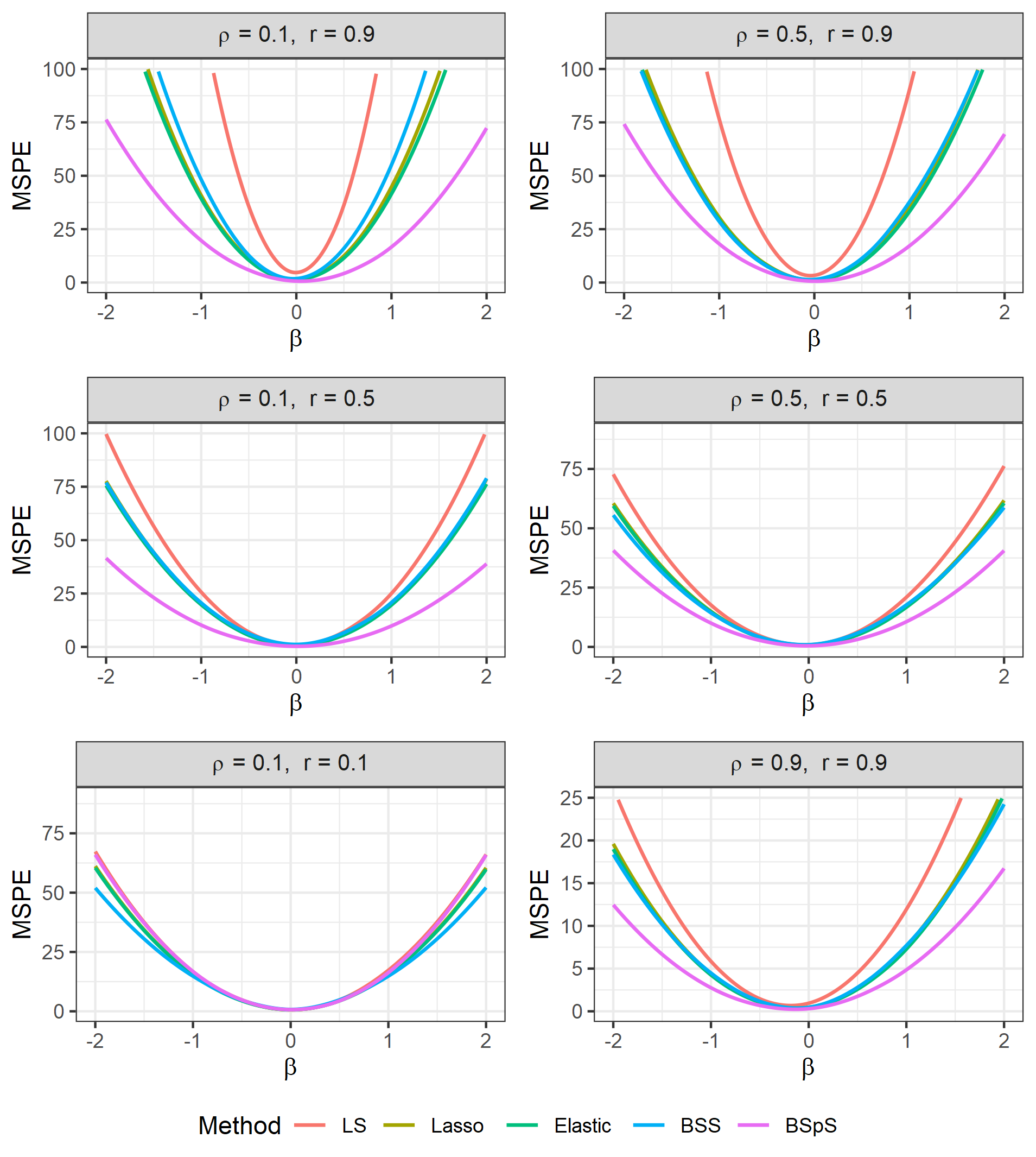
(a) Lowest attainable MSPE curves for the five competitors.

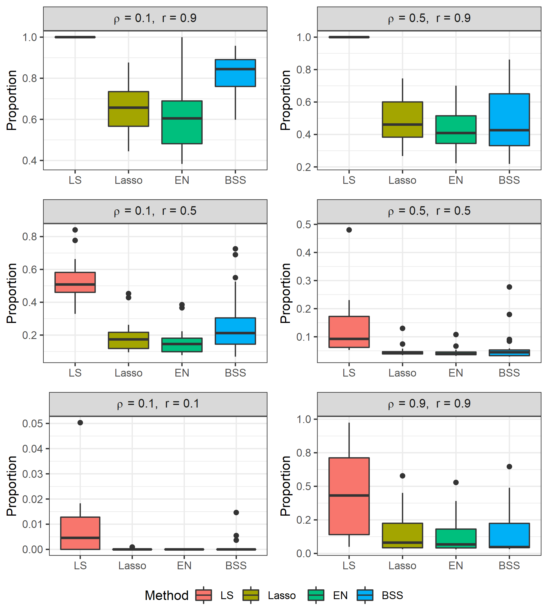
(b) Proportion of splits which yield a lower MSPE than the lowest attainable MSPE of each competitor.

Figure 1: Lowest attainable MSPE for simulation settings with $\text{SNR}=1$.

Figure 1a shows that BSpS often yields a better optimal performance than the competitors. An interesting question is whether there is only one or a few splits that lead to such an excellent performance or there is a substantial number of splits leading to a good performance. To shed light on this, we determine in each setting how many of the 1,093 possible splits considered by BSpS yield an MSPE that is lower than the lowest attainable MSPE for each of the competitors. That is, we calculate the proportion

$$\pi^{*} =\frac{1}{|\mathcal{S}|}\sum_{s\in\mathcal{S}}\mathbb{I}\left(\text{MSPE}(\hat{f}_{s})<\text{MSPE}(\hat{f}^{*})\right),$$

where $\hat{f}_{s}$ is the split estimator for a split $s\in\mathcal{S}$, the set of all considered splits, and $\text{MSPE}(f^{*})$ is the lowest attainable performance of the competitor (LS, Lasso, EN or BSS). The panels in Figure 1b show for each of the four competitors a boxplot of the proportions $\pi^{*}$ over the considered range of $\beta$ values. It can be seen that in cases with spurious correlation in the training data, not only the lowest attainable MSPE of BSpS is lower than its competitors, but there is a substantial fraction of splits that yield a lower MSPE than the lowest attainable MSPE of the competitors.

3.3 Cross-Validated Configurations

In practice the optimal value of the regularization parameter $\lambda$ in Lasso/EN or the optimal subset/split $s$ in BSS/BSpS needs to be estimated from the data. Often a validation set is not available and the training data need to be used for this purpose as well. CV is the most popular method to estimate the tuning parameter based on the training data. To investigate whether the performance improvement of BSpS can also be achieved in practice, we now compare the performance of the methods when their tuning parameter is chosen by 10-fold CV.

The resulting MSPEs of all methods are compared in Figure 2a for the range of $\beta$ values and for all considered combinations of $\rho$ and $r$. In case of low correlation ($\rho=0.1$) without spurious correlation in the training data ($r=0.1$) all methods still perform very similar. While Lasso, EN and BSpS still outperform LS in all other situations, this is not the case anymore for BSS. Hence, in this case 10-fold CV often selects a suboptimal subset. While all MSPEs are higher than the lowest attainable MSPEs in Figure 1a, BSpS still clearly outperformed its competitors in these situations. The improvement is again larger in cases with spurious correlation or high overall correlation in the training data.

We now examine whether the good performance of BSpS is due to a small fraction of the datasets where it performs much better than its competitors or holds generally over many datasets in the simulation. Therefore, in each setting we calculate for each competitor the proportion of datasets for which it is outperformed by BSpS, given by

$$\hat{\pi} =\frac{1}{N}\sum_{i=1}^{N}\mathbb{I}\left(\text{MSPE}(\hat{f}_{\hat{s}}^{(i)})<\text{MSPE}(\hat{f}_{\text{CV}}^{(i)})\right),$$ (14)

where for each training dataset $\mathcal{D}^{(i)}\ (1\leq i\leq N)$, $\hat{f}_{\hat{s}}^{(i)}$ is the BSpS estimate corresponding to the optimal split $\hat{s}$ selected by 10-fold CV. Moreover, $\hat{f}_{\text{CV}}^{(i)}$ is either the least squares estimate, the Lasso/EN estimate $\hat{f}_{\hat{\lambda}}^{(i)}$ with $\hat{\lambda}$ selected by 10-fold CV, or the BSS estimate $\hat{f}_{\hat{s}}^{(i)}$ with $\hat{s}$ selected by 10-fold CV.

The panels in Figure 2b show for each of the four competitors a boxplot of the proportions $\hat{\pi}$ over the considered range of $\beta$ values. It can immediately be seen that except for the case $(\rho,r)=(0.1,0.1)$, the proportion of datasets where BSpS outperformed each competitor is very high with the median above 0.70 in all situations. It is interesting to note that while the proportion of splits with MSPE lower than the lowest attainable MSPE of its competitors in Figure 1b was small for the cases $(\rho,r)=(0.1,0.5),(0.5,0.5)$ or $(0.9,0.9)$, the proportion of times that BSpS outperforms these competitors when selecting tuning parameters by CV is still very high. This indicates that the BSpS ensemble estimator remains more stable in practice compared to single-model estimators which are more sensitive to the selection of their tuning parameter.

(a) MSPE curves of estimators selected by CV.

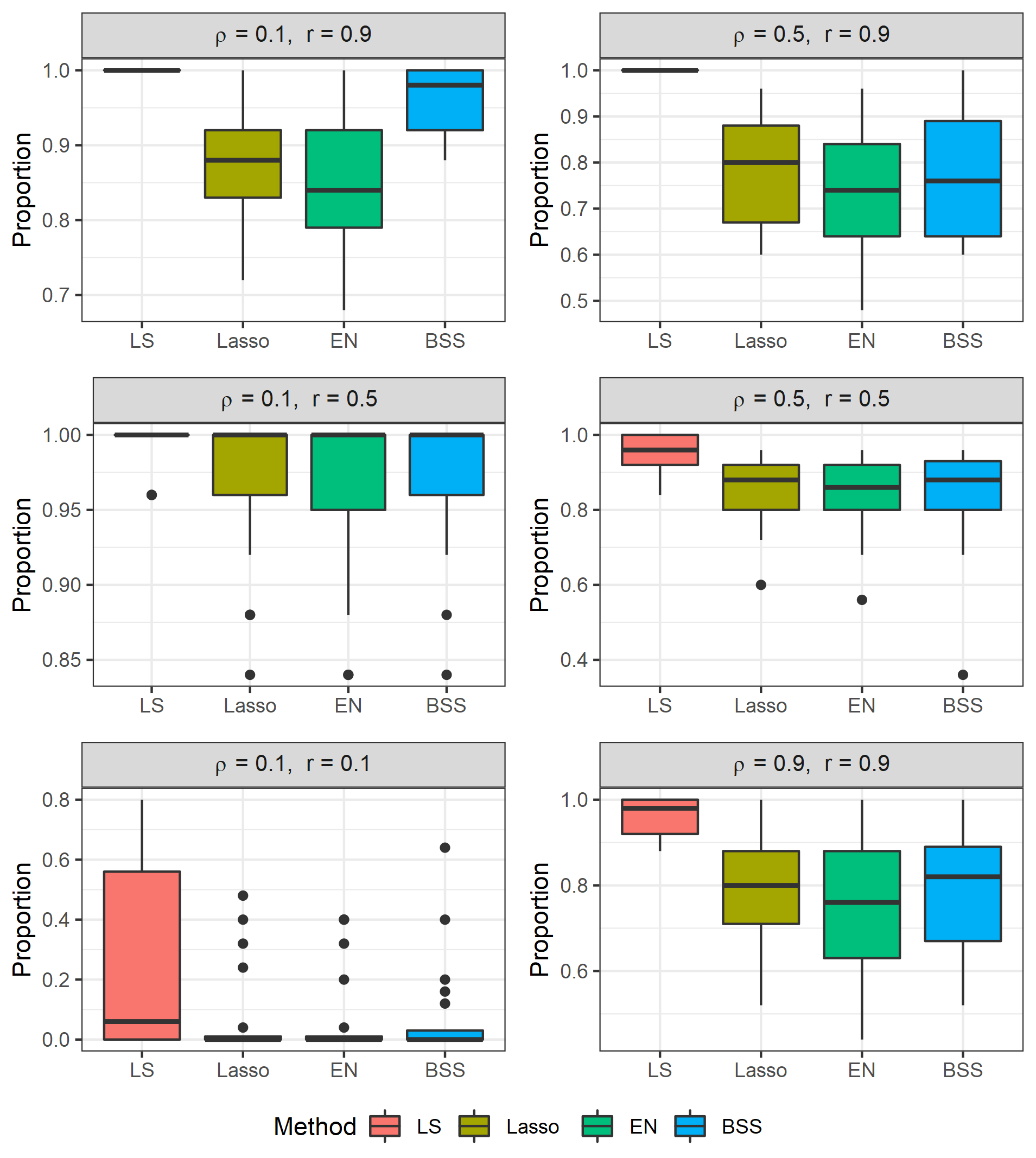
(b) Proportion of BSpS estimates with a lower MSPE than each competitor.

Figure 2: MSPE of estimates obtained by 10-fold CV for simulation settings with $\text{SNR}=1$.

As discussed before, the computation time of BSpS is substantial, and multiplies further when selecting the maximal model size by CV. Therefore, the splitSelect package can make use of multicore parallelization. When using 10-fold CV for the datasets in our simulation setting, the computation time for BSpS in R was on average 8.4 CPU seconds on a 2.7 GHz Intel Xeon processor in a machine running Linux 7.8 with 125 GB of RAM when using 24 cores. Using a single core, the computation time averaged over 3 CPU minutes on the same machine.

3.4 Bias-Variance-Covariance Tradeoff

As explained in the Introduction, ensemble models reach their good performance via the bias-variance trade-off in (4)-(5). For regression ensembles this bias-variance-covariance relation has been studied extensively in Brown et al. (2005). In essence, at the cost of an increase in bias, the PE of a regression ensemble can be greatly reduced by decorrelation of the models in the ensemble.

To investigate the bias-variance-covariance relation in BSpS ensembles, we ran a simulation study to compare LS, BSpS with $G=2$ and BSpS with $G=3$, with $u=0$ and splits chosen by 10-fold CV. We use the simulation design of Section 3.1 with $\beta=1$ in the vector of regression coefficients to measure the average bias, variance and covariance of the models in the ensemble as well as the resulting MSPE.

In Table 1, we report ${\overline{\text{{Bias}}}_{G}^{2}}$, ${\overline{\text{{Var}}}_{G}}$, ${\overline{\text{{Cov}}}_{G}}$ and MSPE of the three methods, averaged over $N=$ 1,000 training sets. Except for the case $(\rho,r)=(0.1,0.1)$, both BSpS ensembles clearly outperform LS in terms of MSPE. While the least squares estimator is unbiased as expected, the BSpS ensembles are biased. However, this bias is combined with a much smaller ensemble variance, due to the contribution of the average covariance between the models in the ensemble which is mostly negative.

Table 1: Average ${\overline{\text{{Bias}}}_{G}^{2}}$, ${\overline{\text{{Var}}}_{G}}$, ${\overline{\text{{Cov}}}_{G}}$ and MSPE for LS and BSpS with $G=2$ and $G=3$ for $\beta=2$ and $\text{SNR}=1$.

	$\mathbf{\overline{\text{{Bias}}}_{G}^{2}}$	$\mathbf{\overline{\text{{Var}}}_{G}}$	$\mathbf{\overline{\text{{Cov}}}_{G}}$	MSPE		$\mathbf{\overline{\text{{Bias}}}_{G}^{2}}$	$\mathbf{\overline{\text{{Var}}}_{G}}$	$\mathbf{\overline{\text{{Cov}}}_{G}}$	MSPE
$\boldsymbol{(\rho,r)=(0.1,0.9)}$					$\boldsymbol{(\rho,r)=(0.5,0.9)}$
LS	0.0	534.6	$-$	534.6	LS	0.0	340.0	$-$	340.0
$\boldsymbol{\text{{BSpS }}(G=2)}$	30.7	340.8	-107.4	147.4	$\boldsymbol{\text{{BSpS }}(G=2)}$	30.7	234.9	-23.9	136.2
$\boldsymbol{\text{{BSpS }}(G=3)}$	70.5	272.7	-53.5	125.8	$\boldsymbol{\text{{BSpS }}(G=3)}$	64.1	200.7	-14.9	121.1
$\boldsymbol{(\rho,r)=(0.1,0.5)}$					$\boldsymbol{(\rho,r)=(0.5,0.5)}$
LS	0.0	102.4	$-$	102.4	LS	0.0	79.5	$-$	79.5
$\boldsymbol{\text{{BSpS }}(G=2)}$	19.3	177.5	-114.4	50.9	$\boldsymbol{\text{{BSpS }}(G=2)}$	28.6	94.6	-26.8	62.5
$\boldsymbol{\text{{BSpS }}(G=3)}$	56.3	135.8	-48.3	69.4	$\boldsymbol{\text{{BSpS }}(G=3)}$	72.4	80.9	-13.2	90.6
$\boldsymbol{(\rho,r)=(0.1,0.1)}$					$\boldsymbol{(\rho,r)=(0.9,0.9)}$
LS	0.0	66.8	$-$	66.8	LS	0.0	39.4	$-$	39.4
$\boldsymbol{\text{{BSpS }}(G=2)}$	54.2	86.1	-50.6	71.9	$\boldsymbol{\text{{BSpS }}(G=2)}$	6.3	39.4	3.7	27.9
$\boldsymbol{\text{{BSpS }}(G=3)}$	102.0	65.8	-21.0	109.9	$\boldsymbol{\text{{BSpS }}(G=3)}$	17.6	38.9	3.0	32.6

In sparse regression, the variance of a model is reduced by restricting the parameter space and thus the contribution of predictors to the regression model. On the other hand, in split regression the variance of the final estimator is controlled through the covariance of the models in the regression ensemble. If there are several models that may potentially explain the relationship between the predictors and the response, the advantage of BSpS is that it can combine good and diverse models in an ensemble with low PE. The simultaneous model building approach in (6) allows to learn from the data an optimal balance between individual model accuracy and diversity between the models.

4 A Multi-Convex Relaxation

As discussed in Section 2 the number of possible splits for BSpS as a function of the number of predictors increases at a very fast rate. Therefore, an exhaustive search over all possible splits is not computationally feasible for high-dimensional applications. A popular way to avoid the computational bottleneck of BSS, is by considering convex relaxations such as the Lasso in (2). Similarly, Christidis et al. (2020) recently introduced the SplitReg method which can be seen as a computationally more attractive, multi-convex relaxation of BSpS. In SplitReg the hard thresholds of BSpS in (6) are replaced by soft thresholds which can be incorporated in the objective function more easily. In detail, SplitReg is a minimizer $\boldsymbol{\beta}=(\boldsymbol{\beta}^{1},\dots,\boldsymbol{\beta}^{G})\in\mathbb{R}^{p\times G}$ of an objective function of the form

$$\mathcal{J}\left(\mathbf{y},\mathbf{X},\boldsymbol{\beta}^{1},\dots,\boldsymbol{\beta}^{g}\right)=\sum_{g=1}^{G}\left\{\frac{1}{2n}\lVert\mathbf{y}-\mathbf{X}\boldsymbol{\beta}^{g}\rVert_{2}^{2}+\lambda_{s}P_{d}\left(\boldsymbol{\beta}^{g}\right)+\frac{\lambda_{d}}{2}\sum_{g\neq h}^{G}P_{d}\left(\boldsymbol{\beta}^{h},\boldsymbol{\beta}^{g}\right)\right\}$$ (15)

where $P_{s}$ and $P_{d}$ are sparsity and diversity penalty functions, and the constants $\lambda_{s},\lambda_{d}>0$, which may be chosen e.g. by CV, control the magnitude of the effect of the sparsity and diversity penalties. Christidis et al. (2020) propose to use as sparsity and diversity penalties

$$P_{s}(\boldsymbol{\beta})=\frac{1-\alpha}{2}\lVert\boldsymbol{\beta}\rVert_{2}^{2}+\alpha\lVert\boldsymbol{\beta}\rVert_{1}\quad\text{ and }\quad P_{d}(\boldsymbol{\beta}^{g},\boldsymbol{\beta}^{h})=\sum_{j=1}^{p}\lvert\boldsymbol{\beta}^{g}\rvert\lvert\boldsymbol{\beta}^{h}\rvert$$ (16)

Hence, $P_{s}(\boldsymbol{\beta})$ is the well-known elastic net penalty while the diversity penalty $P_{d}(\boldsymbol{\beta}^{g},\boldsymbol{\beta}^{h})$ is an $\ell_{1}$-norm relaxation of the hard threshold in (6). Note that for $\lambda_{d}=0$, SplitReg in (15) is equivalent to sparse estimation with the penalty $P_{s}$, irrespective of the number of groups $G$.

The ensemble fit corresponding to the solution of (15) is again given by (7). Christidis et al. (2020) showed that with the penalties in (16) the ensemble estimator yields consistent predictions and has a fast rate of convergence. Moreover, the general framework (15) allows the diversity penalty to be combined with alternative sparsity penalties such as the group Lasso (Yuan and Lin, 2006) for categorical variables or the fused Lasso (Tibshirani et al., 2005) for data containing spatial or temporal structures. The SplitReg objective function is multi-convex and can be solved efficiently via a block coordinate descent algorithm. The number of groups $G$ may be selected in a data-driven way, e.g. by CV.

SplitReg simultaneously learns a small number of models from the data . On the one hand, the sparsity penalty encourages that each of these models contains a small number of predictors which increases interpretability. On the other hand, the diversity penalty encourages diversity between the models such that potentially different mechanisms to explain the response are uncovered. SplitReg thus keeps these advantages of BSpS and at the same time is computationally much more feasible.

To investigate to what extent SplitReg retains the excellent performance of BSpS, we compare the MSPEs of SplitReg and BSpS using the simulation design in subsection 3.1. SplitReg is computed by using the R package SplitGLM (Christidis et al., 2021) where we consider both $G=2$ and $G=3$ groups. We include in our comparisons the fully diverse (FD) SplitReg estimator where $\lambda_{d}=\infty$ is fixed and $\lambda_{s}$ is the only tuning parameter, and the standard version of SplitReg where overlap is allowed, i.e. both $\lambda_{s}$ and $\lambda_{d}$ are tuning parameters. The FD SplitReg estimator is of interest because it is closest to our considered version of BSpS which also uses fully diverse models. We also include EN in the comparison which corresponds to the special case $\lambda_{d}=0$ (i.e. no diversity) in (15). This allows us to assess the added benefit of using an ensemble of models compared to a single model fit.

In Figure 3a we compare the performance of the methods by plotting their lowest attainable MSPEs on the test set when varying their tuning parameter(s). It can be seen that in nearly all cases BSpS performs best followed by SplitReg, but the difference between both is generally small. EN and FD SplitReg usually perform worse than the standard SplitReg, which is not surprisingly because SplitReg can fully optimize over both tuning parameters. Note that in the case $(\rho,r)=(0.1,0.1)$ SplitReg and EN actually outperform BSpS, which shows that SplitReg is better able to adapt to cases where diverse models are not required.

To further examine the difference between BSpS and its relaxations, we calculate for each setting the proportions of the 1,093 splits considered by BSpS that yield lower MSPE than the optimal MSPE of each of the SplitReg alternatives. In Figure 3b boxplots of these proportions over the grid of $\beta$ values are shown. We can see that in most cases there are only few splits that yield better MSPE than the optimal MSPE for the standard SplitReg while the proportions are often much higher for the two other SplitReg alternatives.

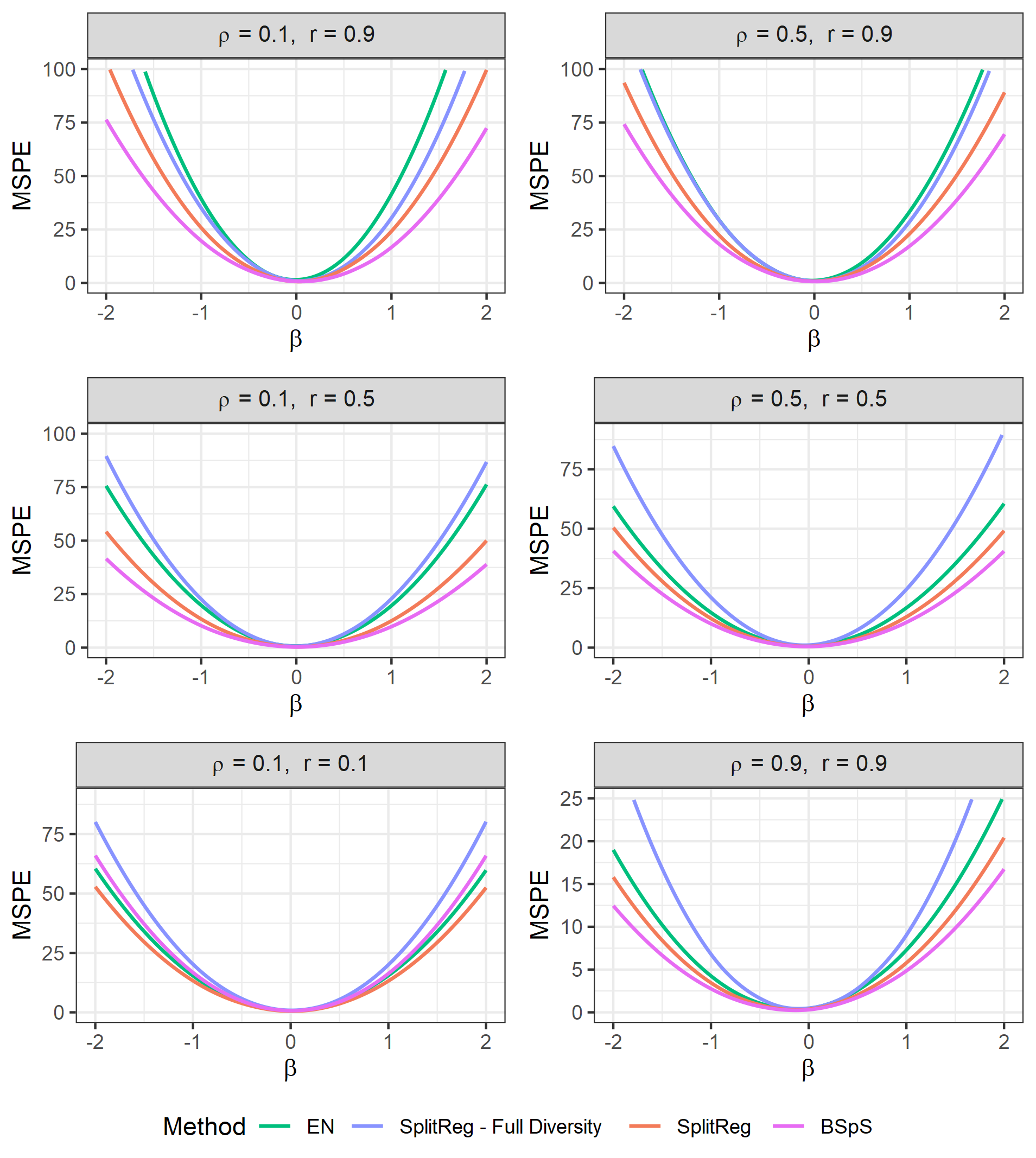
(a) Lowest attainable MSPE curves for the methods.

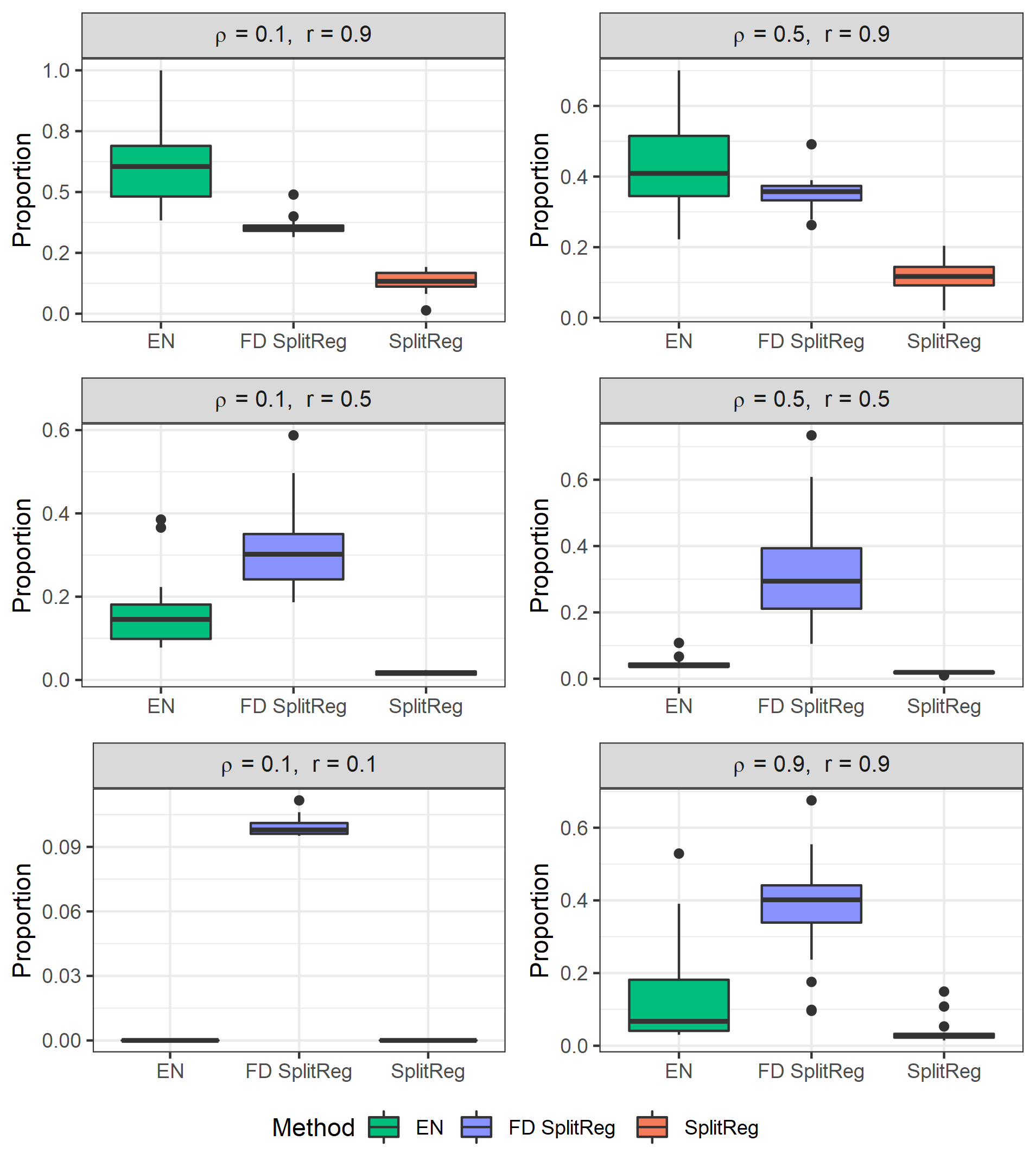
(b) Proportion of splits which yield a lower MSPE than the lowest attainable MSPE of each SplitReg alternative.

Figure 3: Lowest attainable MSPE for BSpS and SplitReg alternatives for simulation settings with $\text{SNR}=1$.

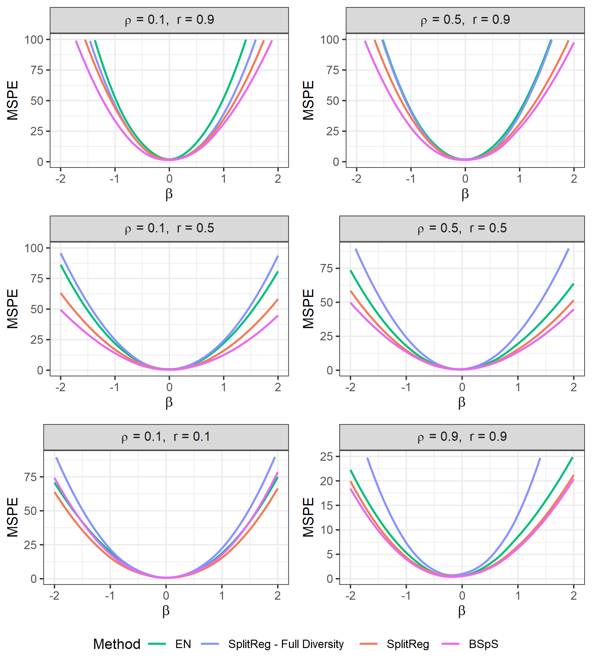
(a) MSPE curves of estimators selected by CV.

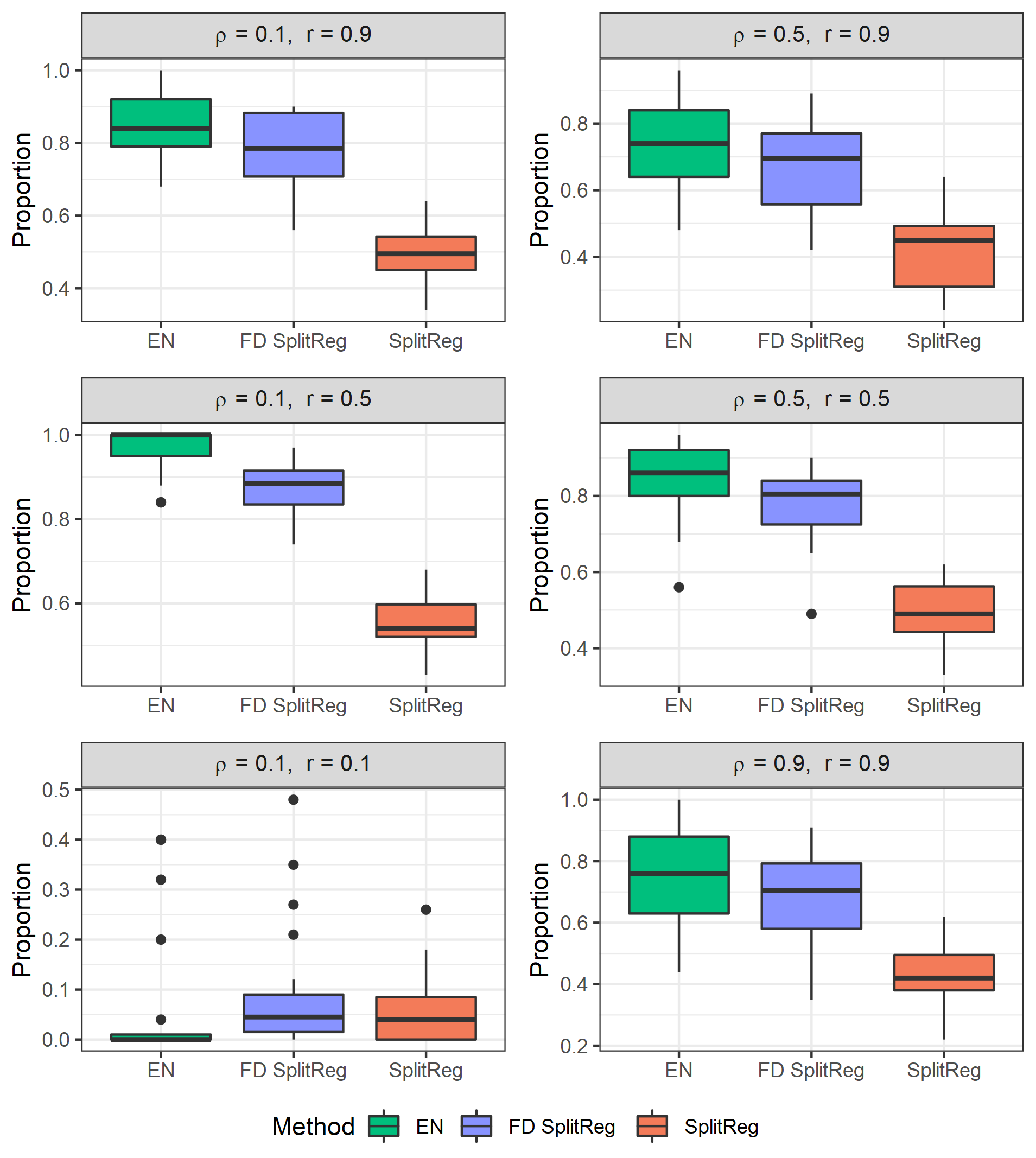
(b) Proportion of BSpS estimates with a lower MSPE than each SplitReg alternative.

Figure 4: MSPE of BSpS and SplitReg estimates obtained by 10-fold CV for simulation settings with $\text{SNR}=1$.

A more practically realistic comparison is obtained if we compare the performance of the methods when the training data are used to select the values of their tuning parameters. Therefore, we compare the MSPE of the methods when their tuning parameters ($\lambda_{s},\lambda_{d}$, $G\in\{2,3\}$ for SplitReg and $s\in\mathcal{S}$ for BSpS) are chosen by 10-fold CV. It can be seen from Figure 4a that the difference in MSPE between SplitReg and BSpS remains very small, confirming again that SplitReg provides a good approximation of the BSpS solution. To examine further to what extent BSpS outperforms its multi-convex relaxations, we calculate for each SplitReg alternative the proportion of datasets for which it is outperformed by BSpS as in (14). The panels in Figure 4b show boxplots of these proportions over the considered range of $\beta$ values for each of the SplitReg alternatives. It can be seen that the proportions are much smaller for standard SplitReg compared to EN and fully diverse SplitReg.

The standard SplitReg which constructs multiple models that are allowed to overlap while penalizing diversity performed better than both EN and FD SplitReg. This reveals that also for the multi-convex relaxations performance can be improved by considering multiple models in an ensemble rather than estimating a single model such as EN. It also indicates that next to the fully diverse splits considered by BSpS, there likely are several splits which share predictors that also yield good prediction performance, and SplitReg is able to exploit this in a computationally tractable way.

5 Discussion

In split regression, a small number of sparse and diverse models are learned simultaneously from the data. Similarly to sparse regression it yields a highly interpretable solution but at the same time split regression ensembles can yield a considerably higher prediction accuracy than single model estimators. Moreover, each of the models for the ensemble describes a possible mechanism that relates the predictor variables to the response and thus can provide more insight than a single model.

To investigate the usefulness of split regression we compared BSpS to standard LS, BSS, Lasso and EN. Due to the high computation time of BSpS for high-dimensional data, we simulated low-dimensional data which mimic the complexities of high-dimensional data such as low SNR and spurious correlations. For such complex data, the best possible MSPE of BSpS is lower than the lowest attainable MSPE of its competitors. Moreover, there are generally many possible splits with a lower MSPE than the lowest attainable MSPE of these competitors. These advantages of BSpS are higher in cases with higher spurious correlations. When the models are tuned via 10-fold CV, BSpS performs even better than its competitors. This is likely due to the fact that there are many splits for BSpS that yield low MSPE while the performance of its competitors is much more sensitive to a good selection of their tuning parameters.

BSpS achieved superior empirical performance despite the fact that the data was generated from a single linear model, which would be expected to favor the single-model competitors. Examining the bias-variance-covariance trade-off for BSpS revealed that by simultaneously learning the models from the data, the method selects models with a good balance between individual model accuracy and diversity. Combining these models yields an ensemble with a small variance, resulting in a low prediction error.

The simulation design, which served as a proxy for high-dimensional data, provides strong empirical evidence that BSpS would be beneficial for high-dimensional data, but the method is too computationally demanding. Therefore, we considered SplitReg, a multi-convex relaxation of BSpS which is computationally more tractable and still interpretable. The lowest attainable MSPE of SplitReg was close to the MSPE of BSpS and the difference remained small when both models were tuned via CV. This illustrates that computationally tractable methods to simultaneously learn a set of sparse and diverse models from the data provide applied researchers with a very powerful data analysis tool. We hope that this article will motivate further research in this new exciting field with great potential for data analysis tasks in high-dimensional settings.

An interesting direction for further research is the development of alternative relaxations to learn a set of sparse and diverse models from the data. While we considered ensembling linear models, the split modeling framework is very general and can be applied in many other settings. For example, the idea can easily be used to construct classifier ensembles, or ensembles of generalized linear models.

The R packages splitSelect, simTargetCov and SplitGLM created for this article are publicly available on CRAN together with their respective reference manuals. The scripts to replicate all simulation studies in this article are available at https://doi.org/10.5281/zenodo.5598086.

Appendix A Low SNR Results

We replicate the simulations in Sections 3 and 4 for $\text{SNR}=0.5$, which yields the following results.

A.1 Low SNR Results for Section 3.2

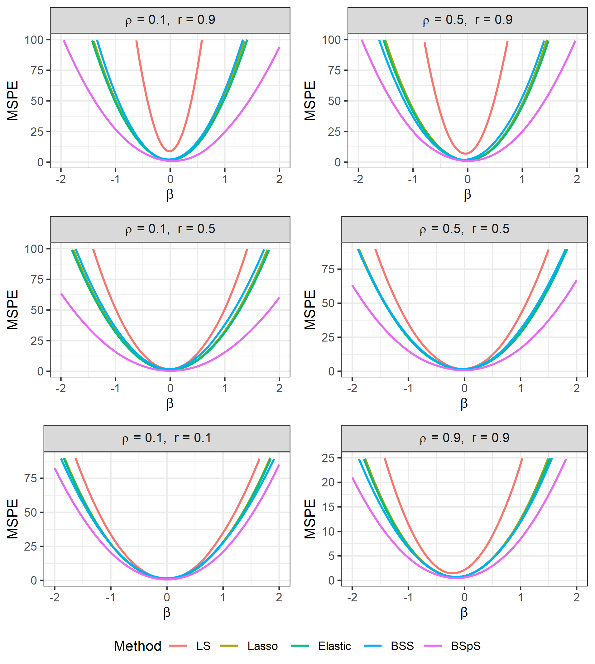
(a) Lowest attainable MSPE curves for the five competitors.

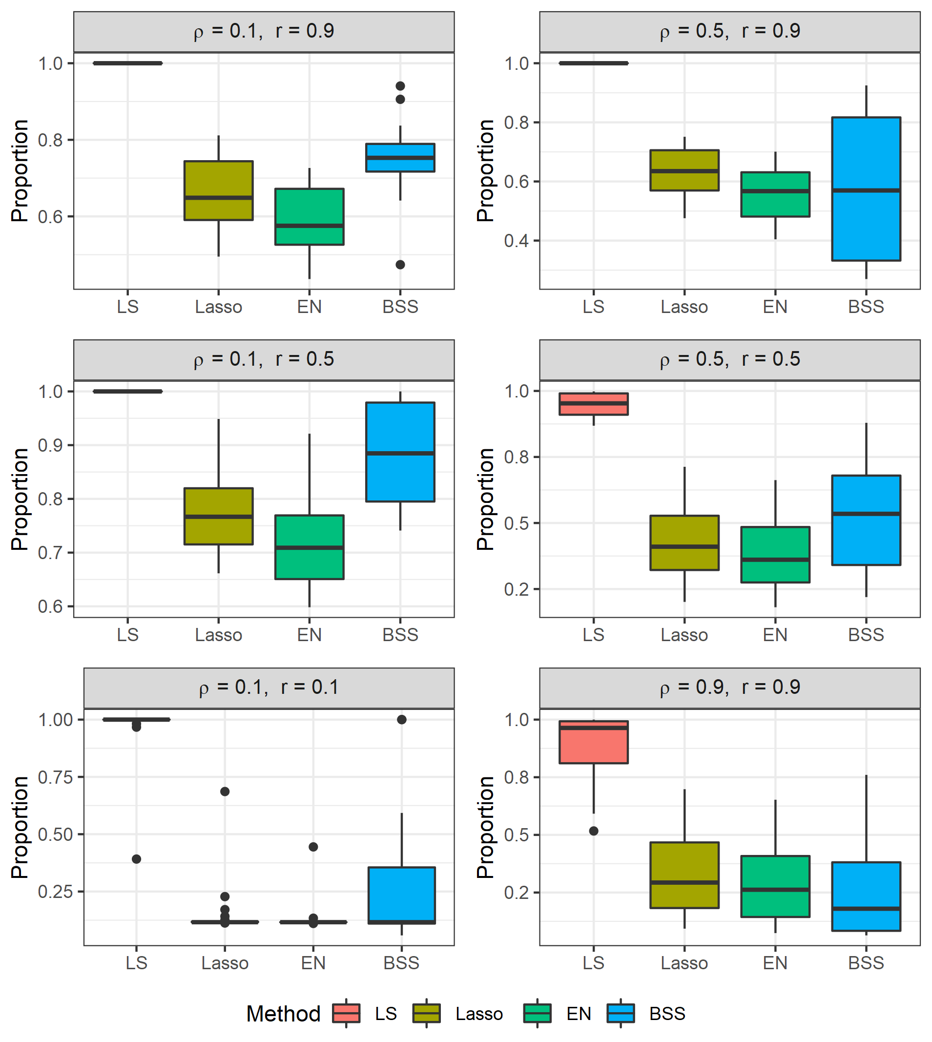
(b) Proportion of splits which yield a lower MSPE than the lowest attainable MSPE of each competitor.

Figure 5: Lowest attainable MSPE for simulation settings with $\text{SNR}=0.5$.

A.2 Low SNR Results for Section 3.3

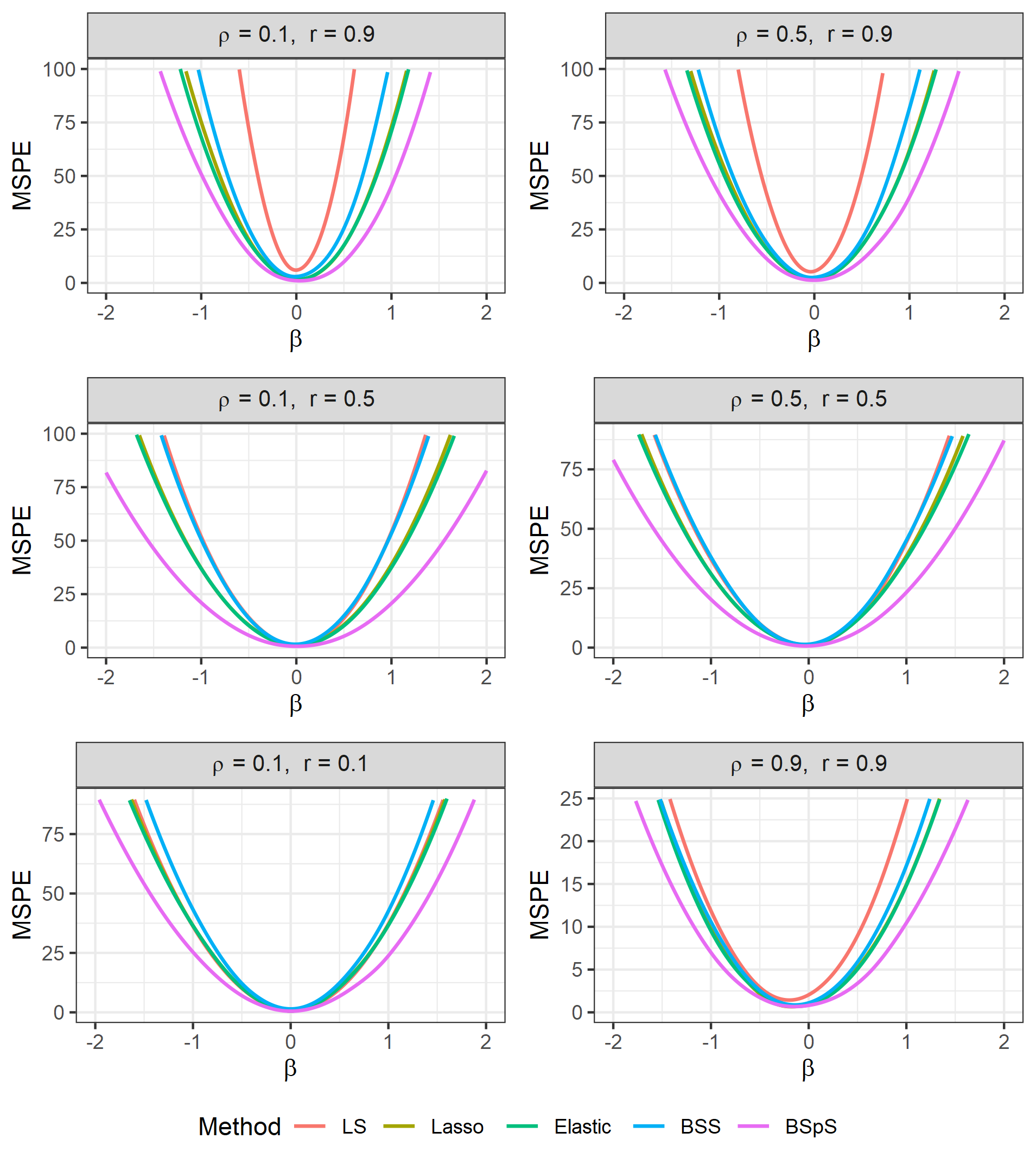
(a) MSPE curves of estimators selected by CV.

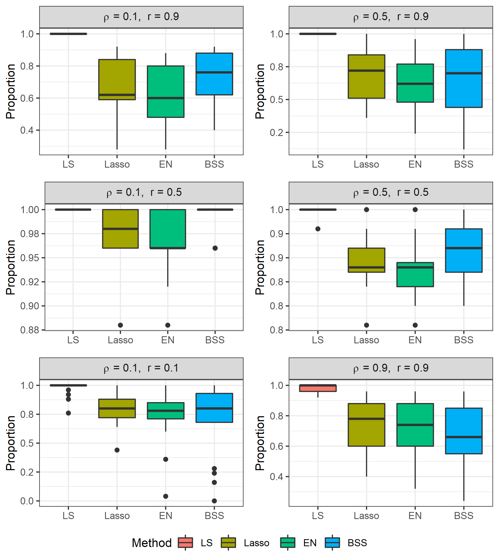
(b) Proportion of BSpS estimates with a lower MSPE than each competitor.

Figure 6: MSPE of estimates obtained by 10-fold CV for simulation settings with $\text{SNR}=0.5$.

A.3 Low SNR Results for Section 3.4

Table 2: Average ${\overline{\text{{Bias}}}_{G}^{2}}$, ${\overline{\text{{Var}}}_{G}}$, ${\overline{\text{{Cov}}}_{G}}$ and MSPE for LS and BSpS with $G=2$ and $G=3$ for $\beta=2$ and $\text{SNR}=0.5$.

	$\mathbf{\overline{\text{{Bias}}}_{G}^{2}}$	$\mathbf{\overline{\text{{Var}}}_{G}}$	$\mathbf{\overline{\text{{Cov}}}_{G}}$	MSPE		$\mathbf{\overline{\text{{Bias}}}_{G}^{2}}$	$\mathbf{\overline{\text{{Var}}}_{G}}$	$\mathbf{\overline{\text{{Cov}}}_{G}}$	MSPE
$\boldsymbol{(\rho,r)=(0.1,0.9)}$					$\boldsymbol{(\rho,r)=(0.5,0.9)}$
LS	0.0	931.3	$-$	931.3	LS	0.0	595.8	$-$	595.8
$\boldsymbol{\text{{BSpS }}(G=2)}$	53.5	552.4	-70.0	294.7	$\boldsymbol{\text{{BSpS }}(G=2)}$	43.5	397.1	31.4	257.8
$\boldsymbol{\text{{BSpS }}(G=3)}$	86.0	420.3	-45.5	195.7	$\boldsymbol{\text{{BSpS }}(G=3)}$	75.1	306.2	4.5	180.2
$\boldsymbol{(\rho,r)=(0.1,0.5)}$					$\boldsymbol{(\rho,r)=(0.5,0.5)}$
LS	0.0	181.3	$-$	181.3	LS	0.0	150.9	$-$	150.9
$\boldsymbol{\text{{BSpS }}(G=2)}$	33.9	195.6	-77.7	92.9	$\boldsymbol{\text{{BSpS }}(G=2)}$	36.9	140.4	-10.1	102.0
$\boldsymbol{\text{{BSpS }}(G=3)}$	71.7	159.3	-37.4	99.8	$\boldsymbol{\text{{BSpS }}(G=3)}$	78.5	114.7	-4.1	114.0
$\boldsymbol{(\rho,r)=(0.1,0.1)}$					$\boldsymbol{(\rho,r)=(0.9,0.9)}$
LS	0.0	125.3	$-$	125.3	LS	0.0	75.0	$-$	75.0
$\boldsymbol{\text{{BSpS }}(G=2)}$	58.0	119.9	-49.6	93.1	$\boldsymbol{\text{{BSpS }}(G=2)}$	8.8	63.4	17.8	49.5
$\boldsymbol{\text{{BSpS }}(G=3)}$	104.4	85.3	-19.1	120.2	$\boldsymbol{\text{{BSpS }}(G=3)}$	19.6	57.3	13.8	47.9

A.4 Low SNR Results for Section 4

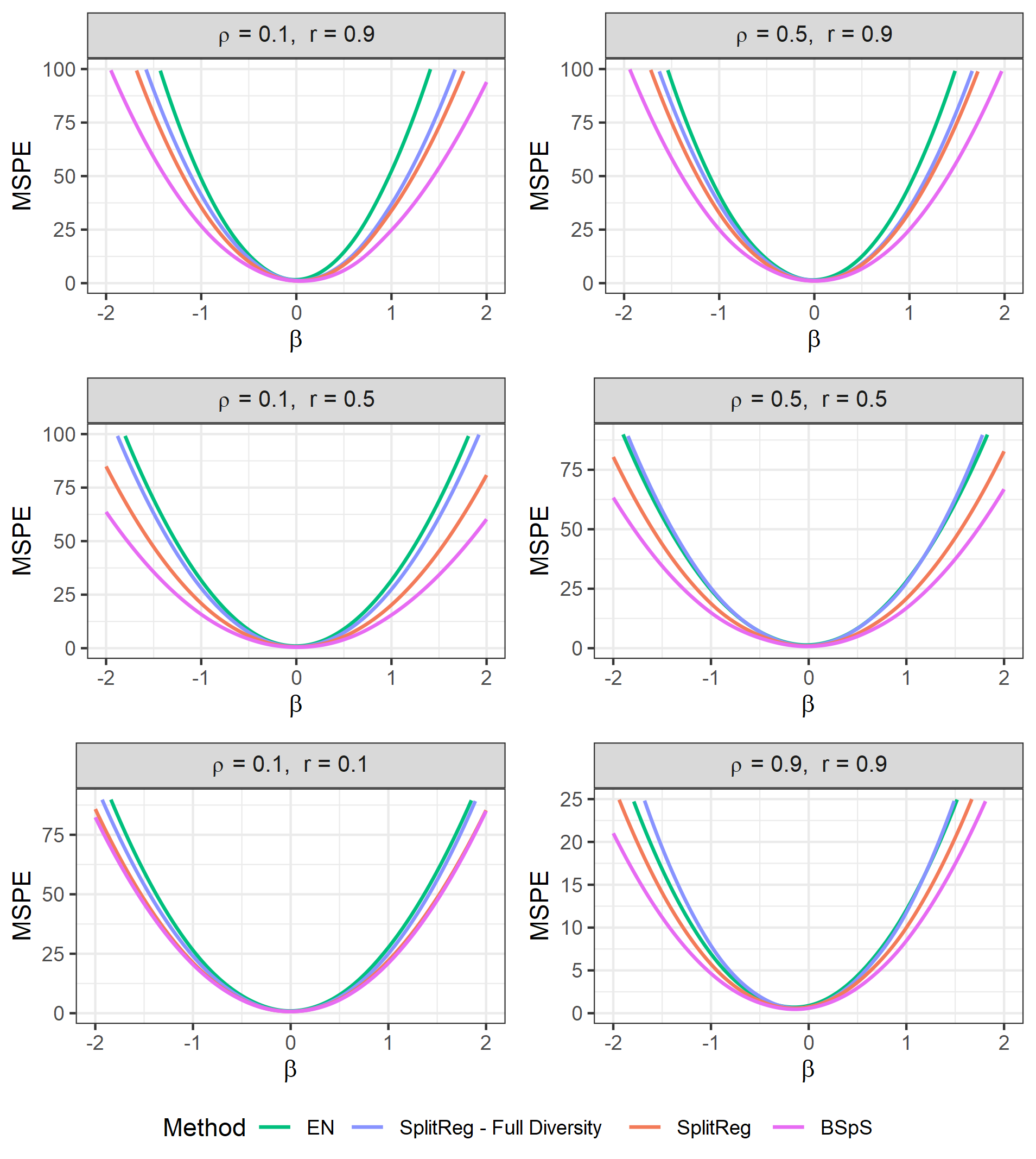
(a) Lowest attainable MSPE curves for the methods.

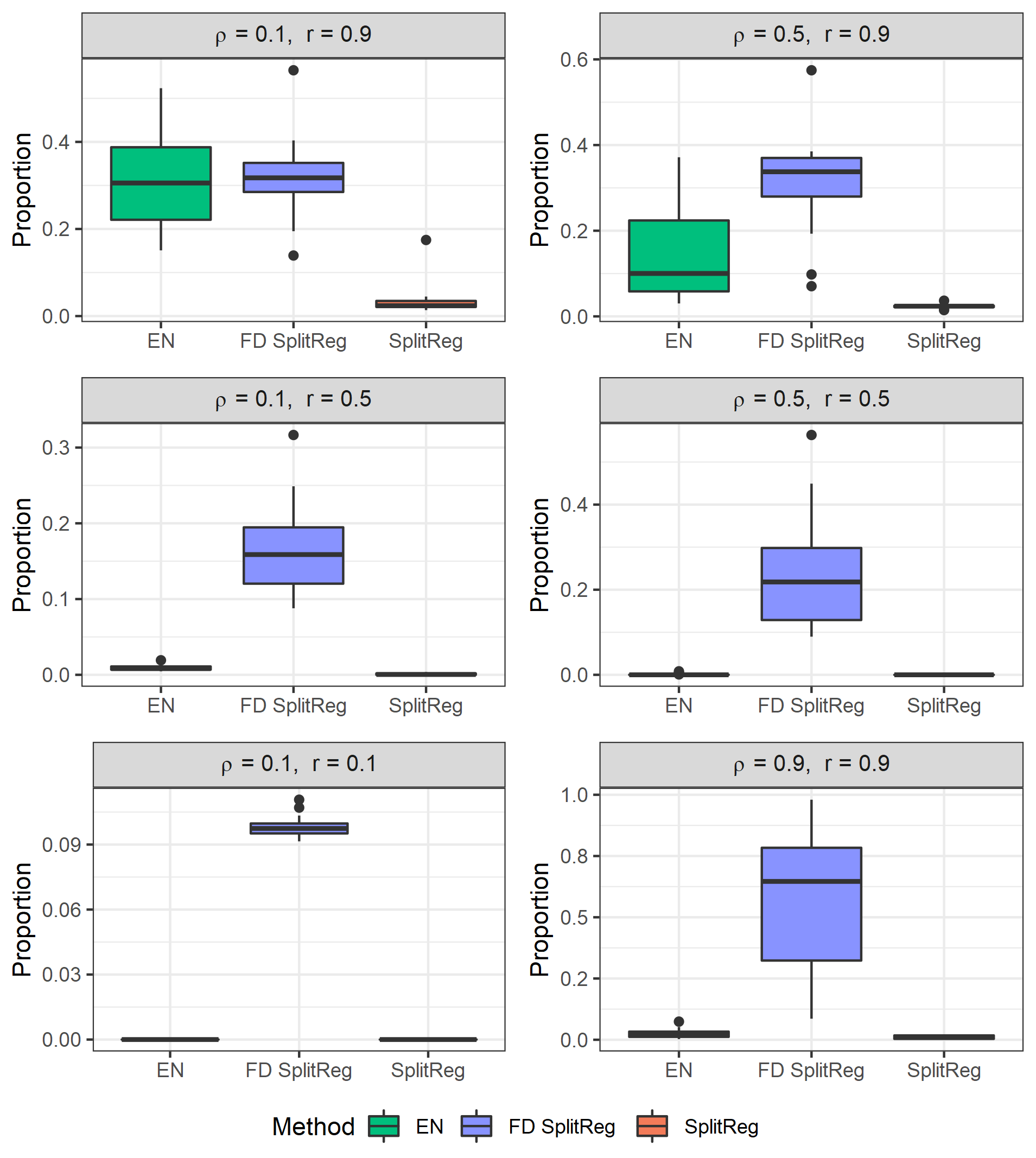
(b) Proportion of splits which yield a lower MSPE than the lowest attainable MSPE of each SplitReg alternative.

Figure 7: Lowest attainable MSPE for BSpS and SplitReg alternatives for simulation settings with $\text{SNR}=0.5$.

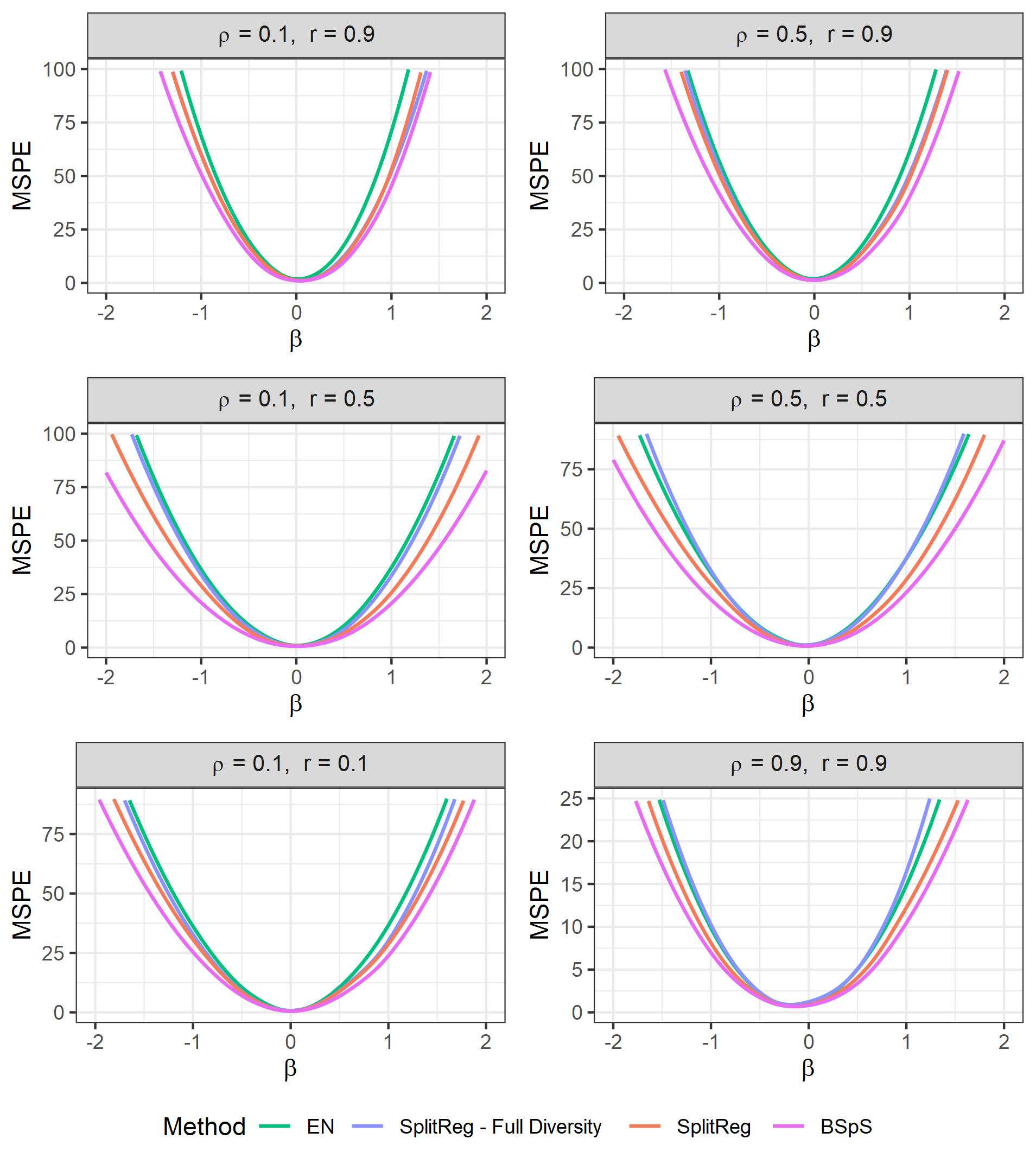
(a) MSPE curves of estimators selected by CV.

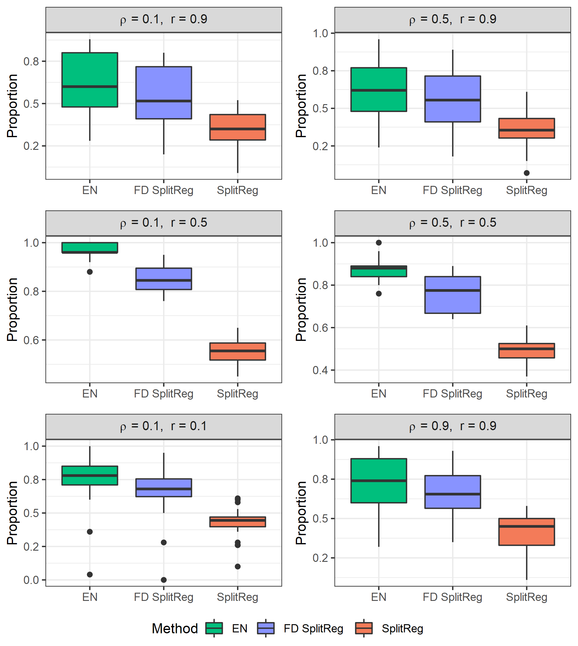
(b) Proportion of BSpS estimates with a lower MSPE than each SplitReg alternative.

Figure 8: MSPE of BSpS and SplitReg estimates obtained by 10-fold CV for simulation settings with $\text{SNR}=0.5$.

Appendix B High SNR Results

We replicate the simulations in Sections 3 and 4 for $\text{SNR}=3$ and $\text{SNR}=5$, which yields the following results.

B.1 High SNR Results for Section 3.2

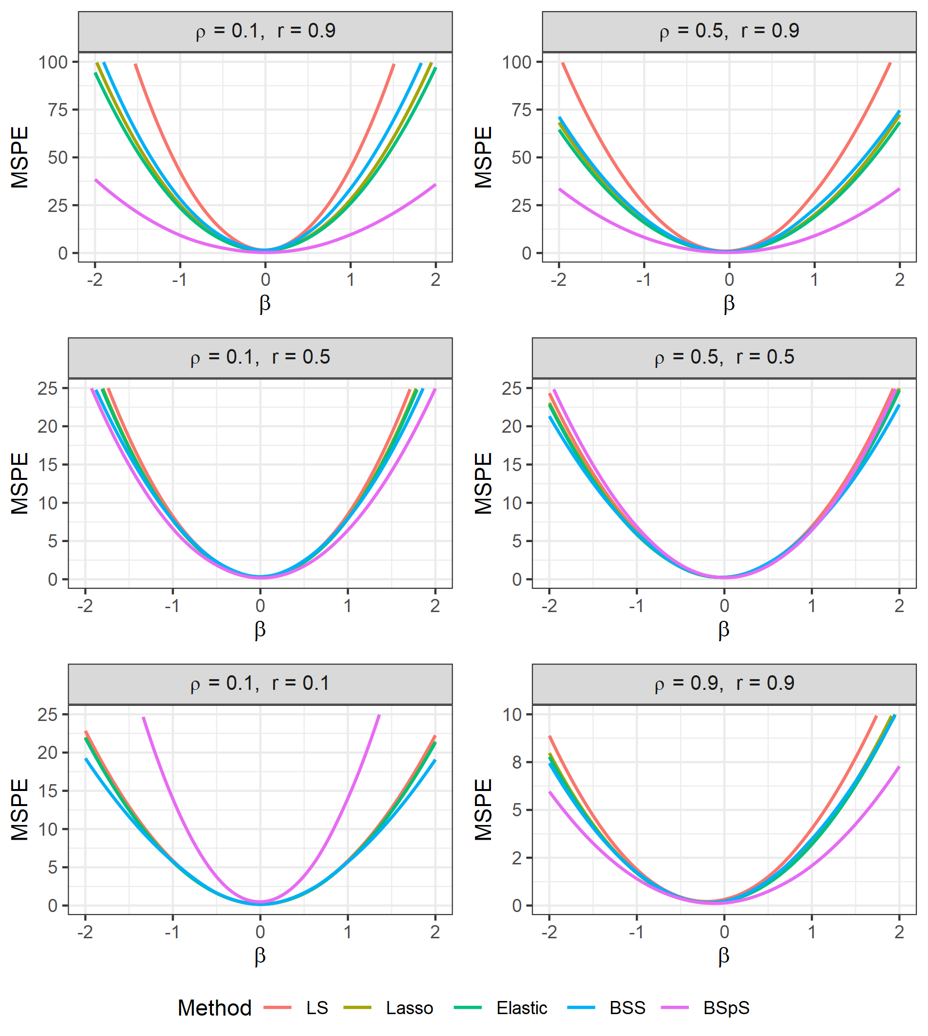
(a) Lowest attainable MSPE curves for the five competitors.

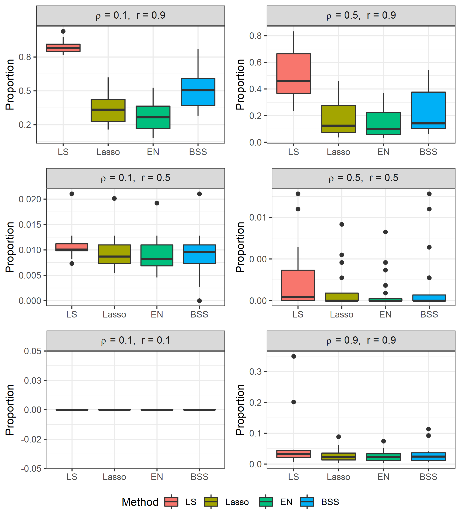
(b) Proportion of splits which yield a lower MSPE than the lowest attainable MSPE of each competitor.

Figure 9: Lowest attainable MSPE for simulation settings with $\text{SNR}=3$.

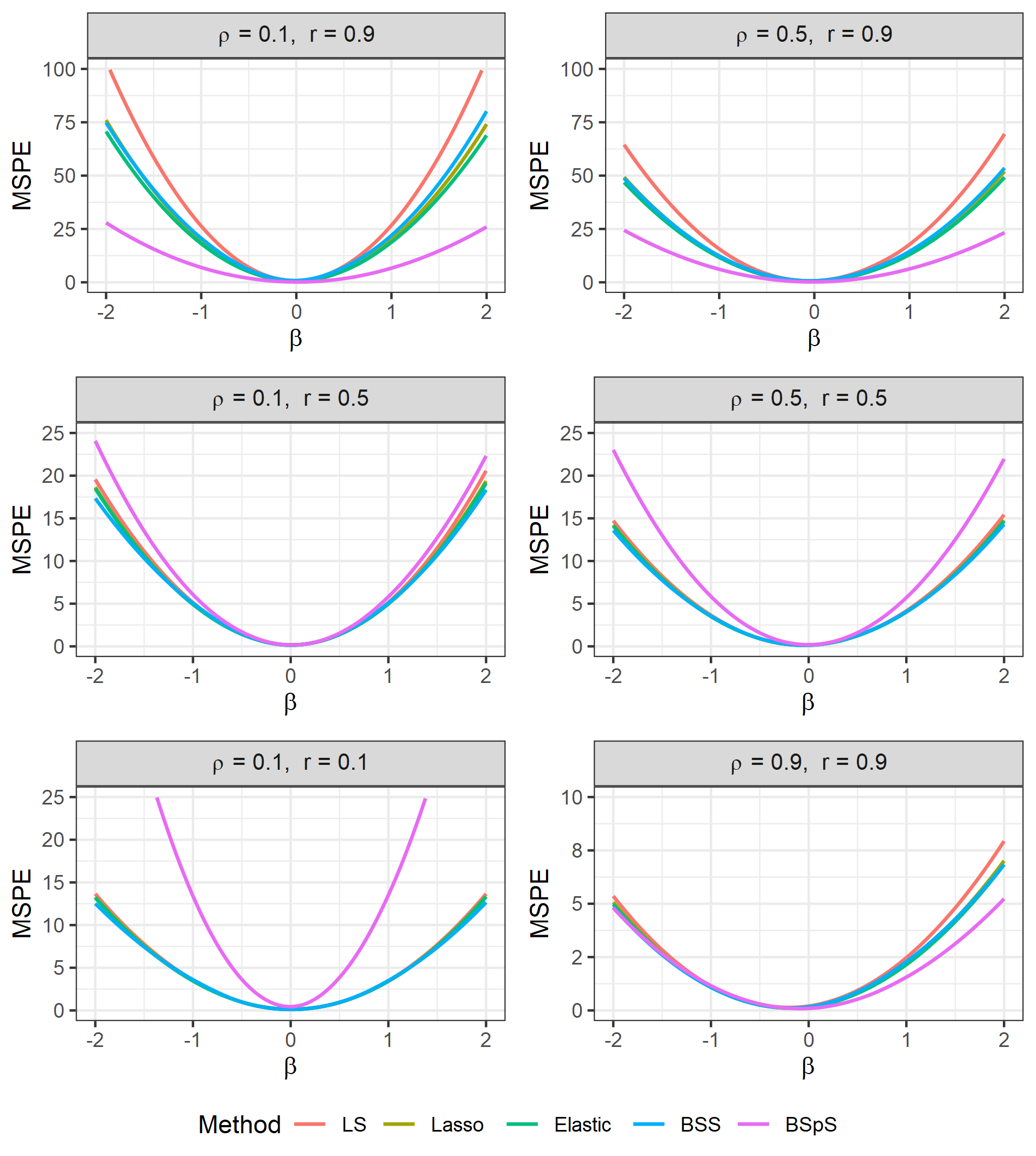
(a) Lowest attainable MSPE curves for the five competitors.

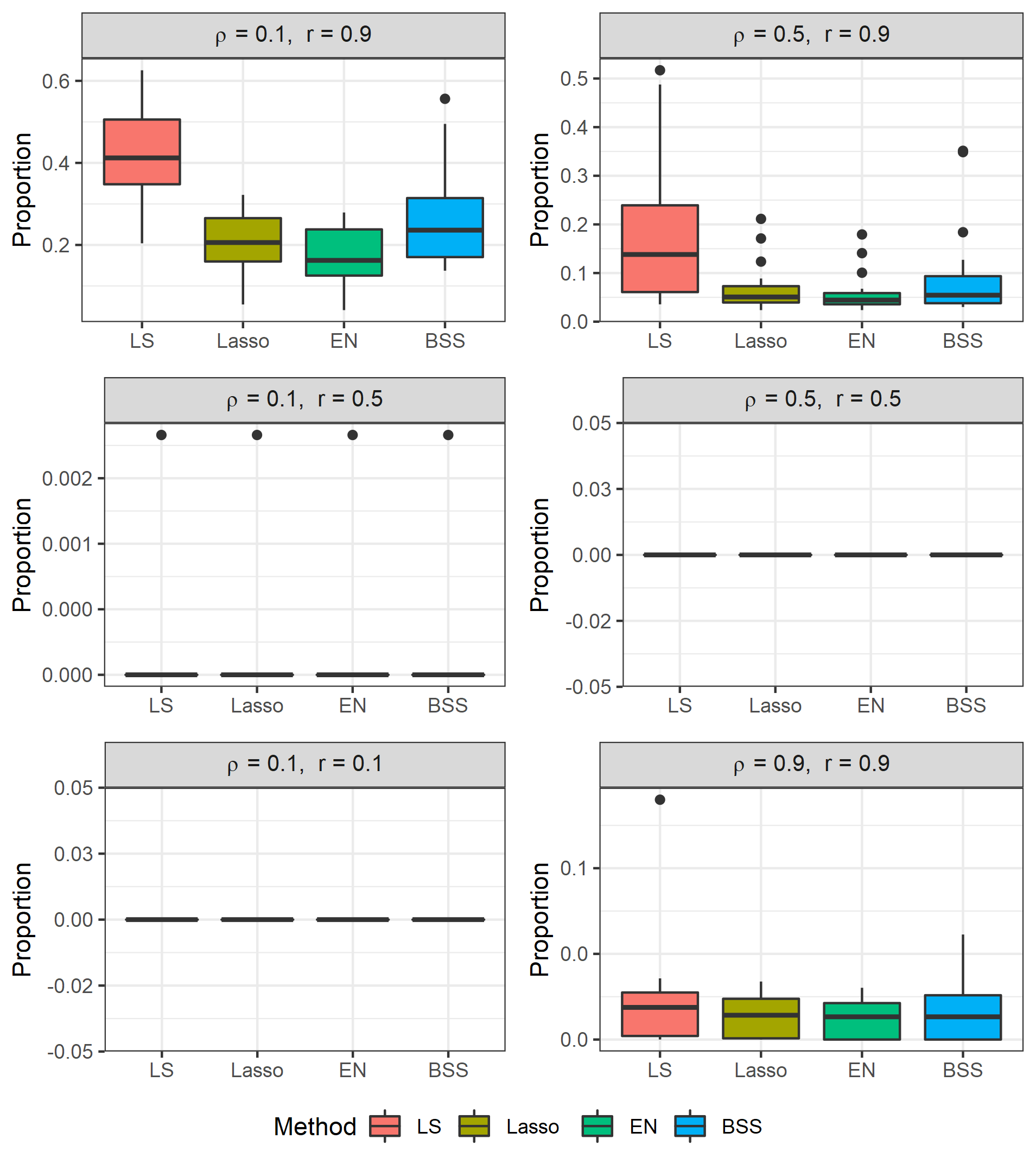
(b) Proportion of splits which yield a lower MSPE than the lowest attainable MSPE of each competitor.

Figure 10: Lowest attainable MSPE for simulation settings with $\text{SNR}=5$.

B.2 High SNR Results for Section 3.3

(a) MSPE curves of estimators selected by CV.

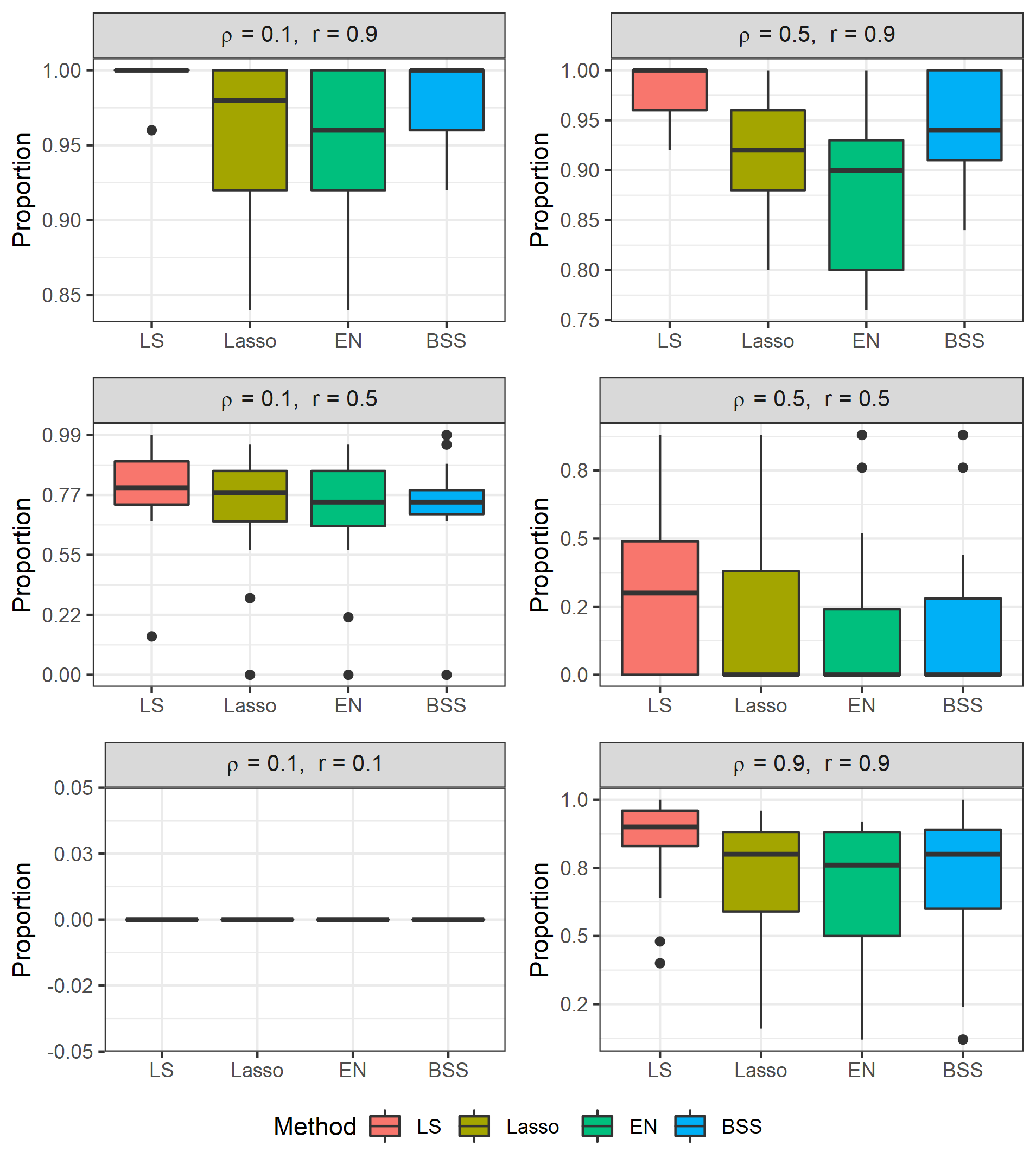
(b) Proportion of BSpS estimates with a lower MSPE than each competitor.

Figure 11: MSPE of estimates obtained by 10-fold CV for simulation settings with $\text{SNR}=3$.

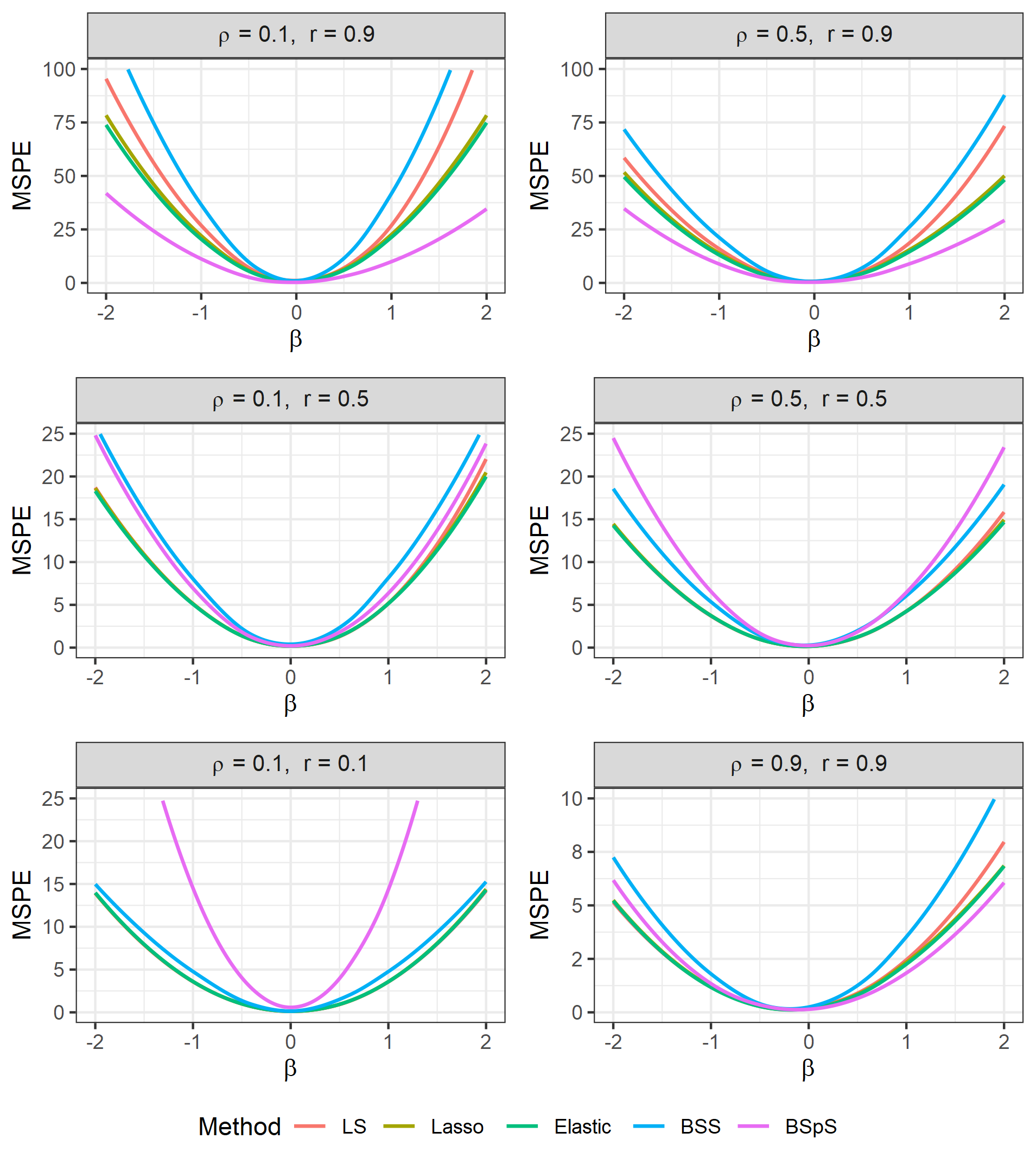
(a) MSPE curves of estimators selected by CV.

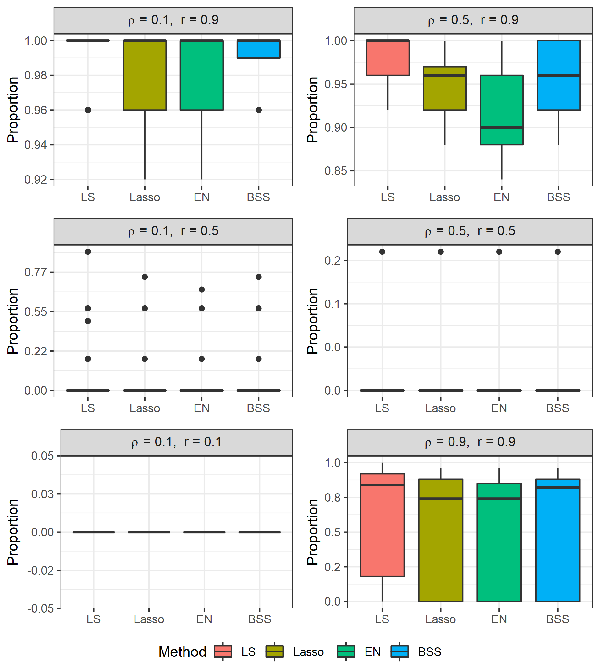
(b) Proportion of BSpS estimates with a lower MSPE than each competitor.

Figure 12: MSPE of estimates obtained by 10-fold CV for simulation settings with $\text{SNR}=5$.

B.3 High SNR Results for Section 3.4

Table 3: Average ${\overline{\text{{Bias}}}_{G}^{2}}$, ${\overline{\text{{Var}}}_{G}}$, ${\overline{\text{{Cov}}}_{G}}$ and MSPE for LS and BSpS with $G=2$ and $G=3$ for $\beta=2$ and $\text{SNR}=3$.

	$\mathbf{\overline{\text{{Bias}}}_{G}^{2}}$	$\mathbf{\overline{\text{{Var}}}_{G}}$	$\mathbf{\overline{\text{{Cov}}}_{G}}$	MSPE		$\mathbf{\overline{\text{{Bias}}}_{G}^{2}}$	$\mathbf{\overline{\text{{Var}}}_{G}}$	$\mathbf{\overline{\text{{Cov}}}_{G}}$	MSPE
$\boldsymbol{(\rho,r)=(0.1,0.9)}$					$\boldsymbol{(\rho,r)=(0.5,0.9)}$
LS	0.0	153.0	$-$	153.0	LS	0.0	99.3	$-$	99.3
$\boldsymbol{\text{{BSpS }}(G=2)}$	17.4	218.1	-123.5	64.7	$\boldsymbol{\text{{BSpS }}(G=2)}$	16.9	127.6	-53.1	54.2
$\boldsymbol{\text{{BSpS }}(G=3)}$	55.4	187.2	-55.2	79.7	$\boldsymbol{\text{{BSpS }}(G=3)}$	54.1	118.1	-26.8	75.6
$\boldsymbol{(\rho,r)=(0.1,0.5)}$					$\boldsymbol{(\rho,r)=(0.5,0.5)}$
LS	0.0	30.2	$-$	30.2	LS	0.0	25.2	$-$	25.2
$\boldsymbol{\text{{BSpS }}(G=2)}$	22.0	123.4	-102.4	32.5	$\boldsymbol{\text{{BSpS }}(G=2)}$	23.3	66.2	-42.9	35.0
$\boldsymbol{\text{{BSpS }}(G=3)}$	60.5	99.6	-43.8	64.5	$\boldsymbol{\text{{BSpS }}(G=3)}$	65.3	54.3	-19.1	70.7
$\boldsymbol{(\rho,r)=(0.1,0.1)}$					$\boldsymbol{(\rho,r)=(0.9,0.9)}$
LS	0.0	20.9	$-$	20.9	LS	0.0	12.5	$-$	12.5
$\boldsymbol{\text{{BSpS }}(G=2)}$	22.0	123.4	-102.4	32.5	$\boldsymbol{\text{{BSpS }}(G=2)}$	23.3	66.2	-42.9	35.0
$\boldsymbol{\text{{BSpS }}(G=3)}$	100.2	49.7	-20.6	103.0	$\boldsymbol{\text{{BSpS }}(G=3)}$	15.8	21.0	-2.2	21.3

Table 4: Average ${\overline{\text{{Bias}}}_{G}^{2}}$, ${\overline{\text{{Var}}}_{G}}$, ${\overline{\text{{Cov}}}_{G}}$ and MSPE for LS and BSpS with $G=2$ and $G=3$ for $\beta=2$ and $\text{SNR}=5$.

	$\mathbf{\overline{\text{{Bias}}}_{G}^{2}}$	$\mathbf{\overline{\text{{Var}}}_{G}}$	$\mathbf{\overline{\text{{Cov}}}_{G}}$	MSPE		$\mathbf{\overline{\text{{Bias}}}_{G}^{2}}$	$\mathbf{\overline{\text{{Var}}}_{G}}$	$\mathbf{\overline{\text{{Cov}}}_{G}}$	MSPE
$\boldsymbol{(\rho,r)=(0.1,0.9)}$					$\boldsymbol{(\rho,r)=(0.5,0.9)}$
LS	0.0	91.8	$-$	91.8	LS	0.0	59.6	$-$	59.6
$\boldsymbol{\text{{BSpS }}(G=2)}$	16.2	186.7	-126.7	46.1	$\boldsymbol{\text{{BSpS }}(G=2)}$	16.3	104.7	-58.3	39.5
$\boldsymbol{\text{{BSpS }}(G=3)}$	53.1	156.2	-54.8	68.6	$\boldsymbol{\text{{BSpS }}(G=3)}$	52.0	95 .1	-27.2	65.6
$\boldsymbol{(\rho,r)=(0.1,0.5)}$					$\boldsymbol{(\rho,r)=(0.5,0.5)}$
LS	0.0	18.1	$-$	18.1	LS	0.0	15.1	$-$	15.1
$\boldsymbol{\text{{BSpS }}(G=2)}$	20.8	117.8	-104.9	27.2	$\boldsymbol{\text{{BSpS }}(G=2)}$	21.9	60.1	-45.9	29.1
$\boldsymbol{\text{{BSpS }}(G=3)}$	59.4	96.3	-44.1	62.2	$\boldsymbol{\text{{BSpS }}(G=3)}$	63.9	51.3	-20.4	67.4
$\boldsymbol{(\rho,r)=(0.1,0.1)}$					$\boldsymbol{(\rho,r)=(0.9,0.9)}$
LS	0.0	12.5	$-$	12.5	LS	0.0	7.5	$-$	7.5
$\boldsymbol{\text{{BSpS }}(G=2)}$	52.8	55.0	-47.0	56.8	$\boldsymbol{\text{{BSpS }}(G=2)}$	3.6	17.5	-8.7	8.0
$\boldsymbol{\text{{BSpS }}(G=3)}$	99.3	48.6	-21.6	101.1	$\boldsymbol{\text{{BSpS }}(G=3)}$	15.2	17.6	-4.0	18.4

B.4 High SNR Results for Section 4

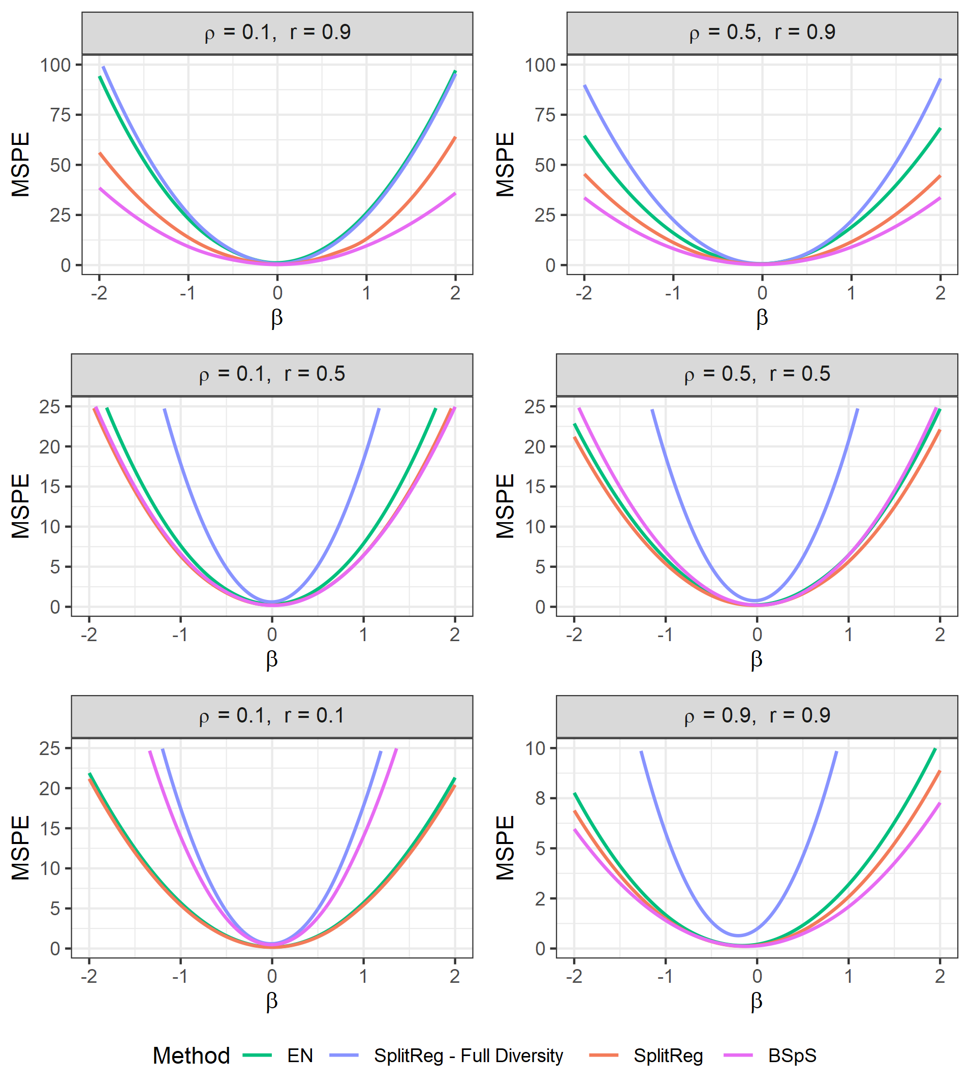
(a) Lowest attainable MSPE curves for the methods.

(b) Proportion of splits which yield a lower MSPE than the lowest attainable MSPE of each SplitReg alternative.

Figure 13: Lowest attainable MSPE for BSpS and SplitReg alternatives for simulation settings with $\text{SNR}=3$.

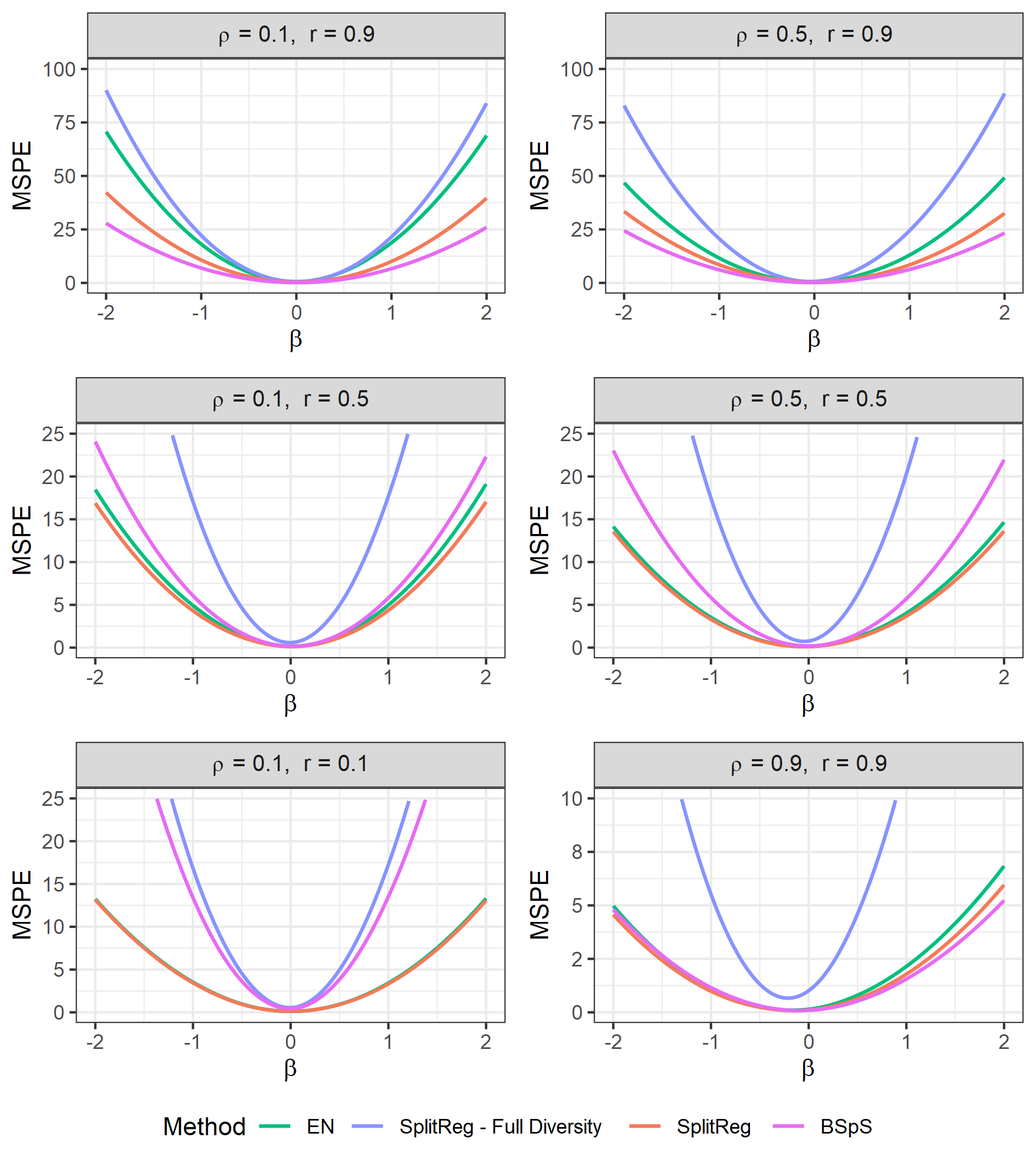
(a) Lowest attainable MSPE curves for the methods.

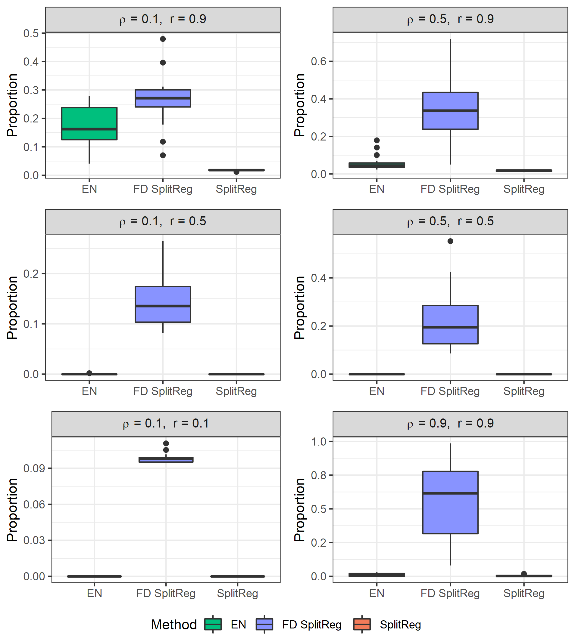
(b) Proportion of splits which yield a lower MSPE than the lowest attainable MSPE of each SplitReg alternative.

Figure 14: Lowest attainable MSPE for BSpS and SplitReg alternatives for simulation settings with $\text{SNR}=5$.

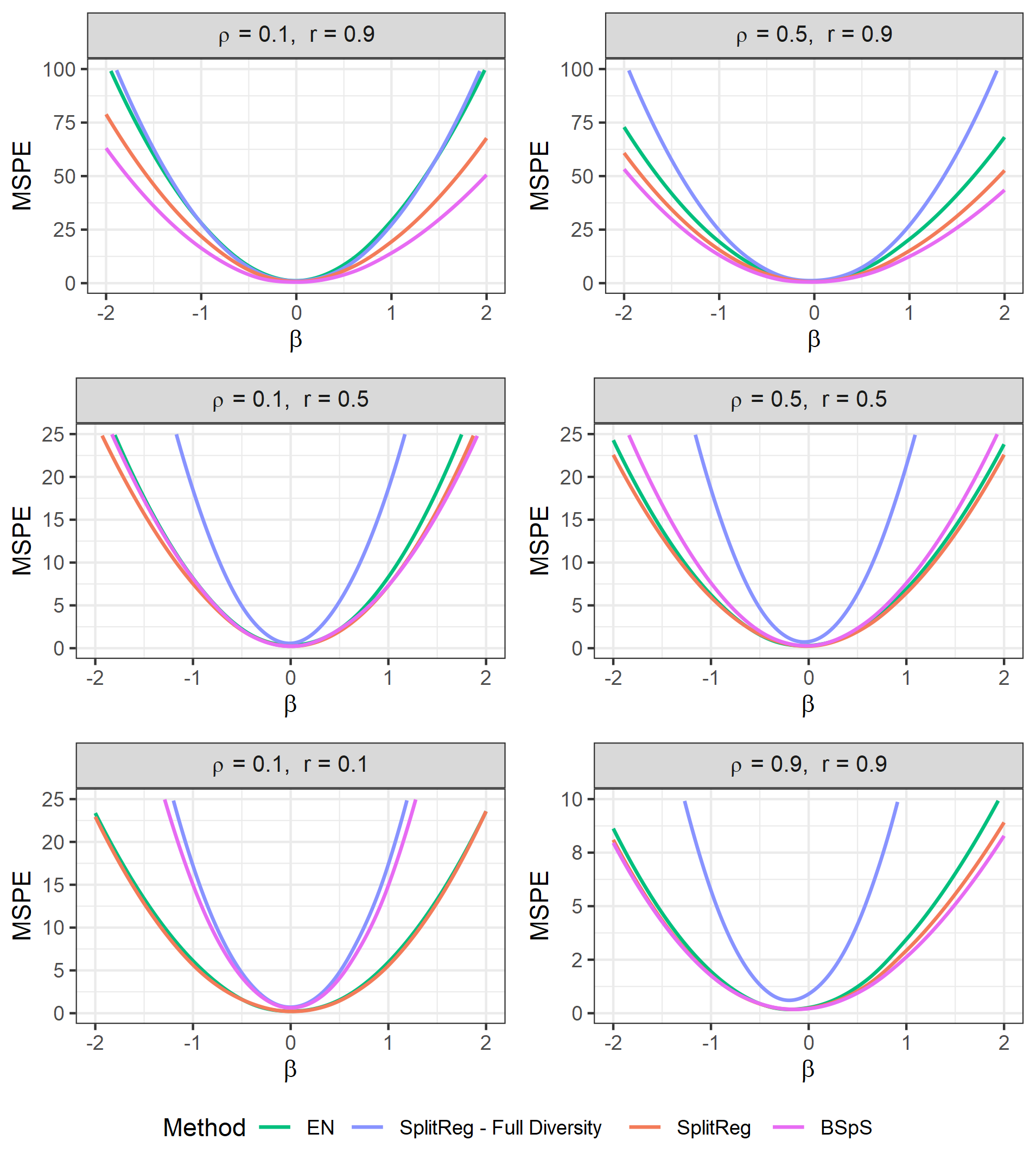
(a) MSPE curves of estimators selected by CV.

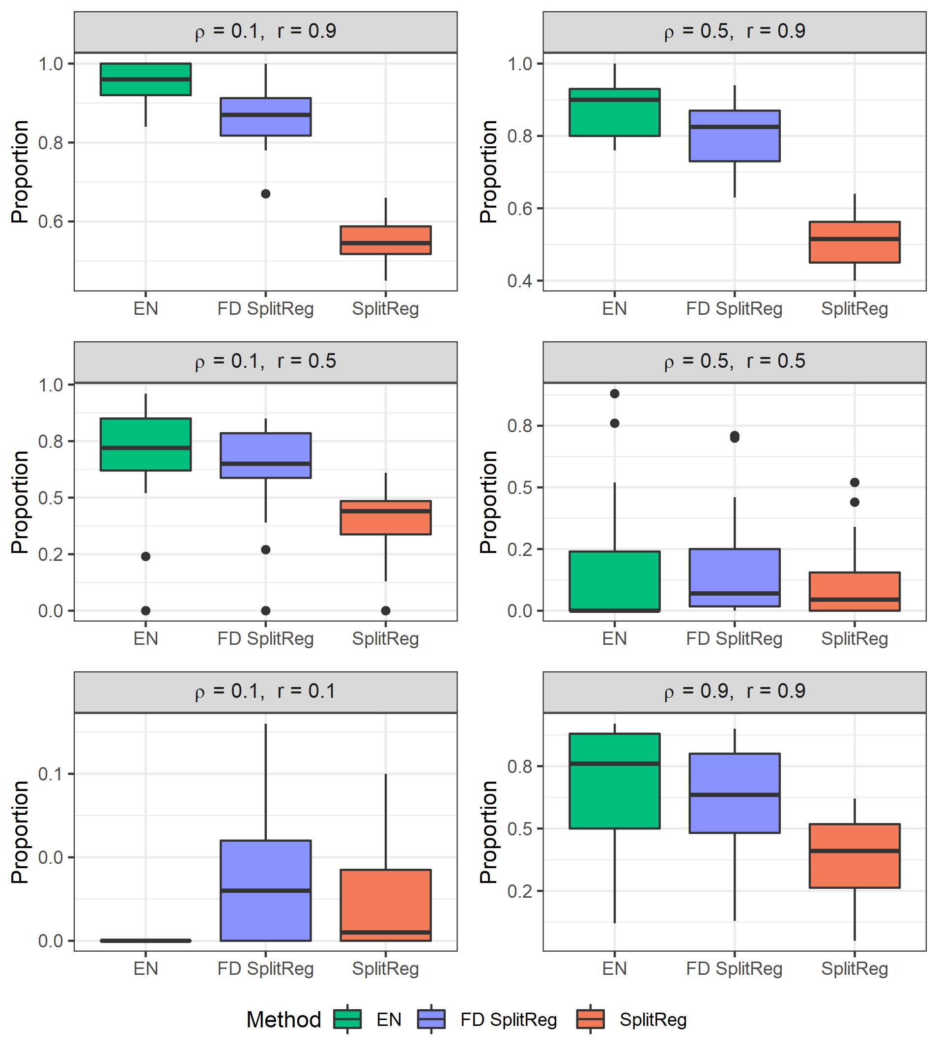
(b) Proportion of BSpS estimates with a lower MSPE than each SplitReg alternative.

Figure 15: MSPE of BSpS and SplitReg estimates obtained by 10-fold CV for simulation settings with $\text{SNR}=3$.

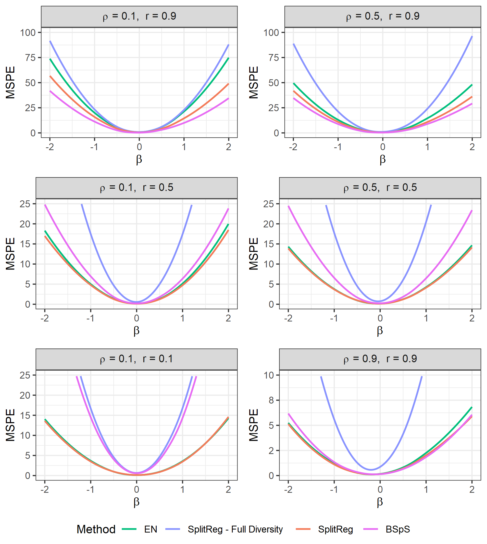
(a) MSPE curves of estimators selected by CV.

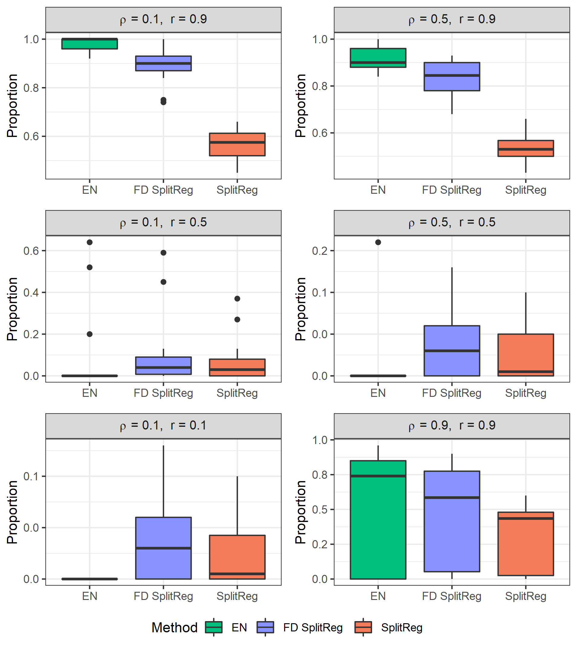
(b) Proportion of BSpS estimates with a lower MSPE than each SplitReg alternative.

Figure 16: MSPE of BSpS and SplitReg estimates obtained by 10-fold CV for simulation settings with $\text{SNR}=5$.

References

- Akaike (1974) Akaike, H. (1974). A new look at the statistical model identification. IEEE transactions on automatic control 19(6), 716–723.
- Amit and Geman (1997) Amit, Y. and D. Geman (1997). Shape quantization and recognition with randomized trees. Neural computation 9(7), 1545–1588.
- Bellman (1956) Bellman, R. (1956). Dynamic programming and lagrange multipliers. Proceedings of the National Academy of Sciences of the United States of America 42(10), 767.
- Bertsimas et al. (2016) Bertsimas, D., A. King, and R. Mazumder (2016). Best subset selection via a modern optimization lens. The annals of statistics 44(2), 813–852.
- Bian and Chen (2021) Bian, Y. and H. Chen (2021). When does diversity help generalization in classification ensembles? IEEE Transactions on Cybernetics.
- Breiman (1995) Breiman, L. (1995). Better subset regression using the nonnegative garrote. Technometrics 37(4), 373–384.
- Breiman (1996) Breiman, L. (1996). Bagging predictors. Machine learning 24(2), 123–140.
- Breiman (2001a) Breiman, L. (2001a, October). Random forests. Machine Learning 45(1), 5–32.
- Breiman (2001b) Breiman, L. (2001b). Statistical modeling: The two cultures (with comments and a rejoinder by the author). Statistical science 16(3), 199–231.
- Brown et al. (2005) Brown, G., J. L. Wyatt, and P. Tiňo (2005). Managing diversity in regression ensembles. Journal of machine learning research 6(Sep), 1621–1650.
- Bühlmann and Yu (2003) Bühlmann, P. and B. Yu (2003). Boosting with the l 2 loss: regression and classification. Journal of the American Statistical Association 98(462), 324–339.
- Bühlmann et al. (2006) Bühlmann, P., B. Yu, Y. Singer, and L. Wasserman (2006). Sparse boosting. Journal of Machine Learning Research 7(6).
- Christidis et al. (2020a) Christidis, A., S. Van Aelst, and R. Zamar (2020a). simTargetCov: Data Transformation or Simulation with Empirical Covariance Matrix. R package version 1.0.1.
- Christidis et al. (2020b) Christidis, A., S. Van Aelst, and R. Zamar (2020b). splitSelect: Best Split Selection Modeling for Low-Dimensional Data. R package version 1.0.1.
- Christidis et al. (2021) Christidis, A., S. Van Aelst, and R. Zamar (2021). SplitGLM: Split Generalized Linear Models. R package version 1.0.2.
- Christidis et al. (2020) Christidis, A.-A., L. Lakshmanan, E. Smucler, and R. Zamar (2020). Split regularized regression. Technometrics 62(3), 330–338.
- Dietterich (2000) Dietterich, T. G. (2000). An experimental comparison of three methods for constructing ensembles of decision trees: Bagging, boosting, and randomization. Machine learning 40(2), 139–157.
- Fan et al. (2012) Fan, J., S. Guo, and N. Hao (2012). Variance estimation using refitted cross-validation in ultrahigh dimensional regression. Journal of the Royal Statistical Society: Series B (Statistical Methodology) 74(1), 37–65.
- Fan and Zhou (2016) Fan, J. and W.-X. Zhou (2016). Guarding against spurious discoveries in high dimensions. The Journal of Machine Learning Research 17(1), 7123–7156.
- Friedman (2001) Friedman, J. H. (2001, 10). Greedy function approximation: A gradient boosting machine. Ann. Statist. 29(5), 1189–1232.
- Friedman et al. (2010) Friedman, J. H., T. Hastie, and R. Tibshirani (2010). Regularization paths for generalized linear models via coordinate descent. Journal of Statistical Software 33(1), 1.
- Hastie et al. (2009a) Hastie, T., R. Tibshirani, and J. Friedman (2009a). Boosting and additive trees. In The elements of statistical learning, pp. 337–387. Springer.
- Hastie et al. (2009b) Hastie, T., R. Tibshirani, and J. Friedman (2009b). Model assessment and selection. In The elements of statistical learning, pp. 219–259. Springer.
- Hastie et al. (2020) Hastie, T., R. Tibshirani, and R. Tibshirani (2020). Best subset, forward stepwise or lasso? analysis and recommendations based on extensive comparisons. Statistical Science 35(4), 579–592.
- Hastie et al. (2019) Hastie, T., R. Tibshirani, and M. Wainwright (2019). Statistical learning with sparsity: the lasso and generalizations. Chapman and Hall/CRC.
- Hazimeh and Mazumder (2020) Hazimeh, H. and R. Mazumder (2020). Fast best subset selection: Coordinate descent and local combinatorial optimization algorithms. Operations Research 68(5), 1517–1537.
- Ho (1998) Ho, T. K. (1998). The random subspace method for constructing decision forests. IEEE transactions on pattern analysis and machine intelligence 20(8), 832–844.
- Mallows (1973) Mallows, C. L. (1973). Some comments on cp. Technometrics 15(4), 661–675.
- McCullagh and Nelder (1989) McCullagh, P. and J. A. Nelder (1989). Monographs on statistics and applied probability. Generalized linear models 37.
- Mountain and Hsiao (1989) Mountain, D. and C. Hsiao (1989). A combined structural and flexible functional approach for modeling energy substitution. Journal of the American Statistical Association 84(405), 76–87.
- Nelder and Mead (1965) Nelder, J. A. and R. Mead (1965). A simplex method for function minimization. The computer journal 7(4), 308–313.
- R Core Team (2021) R Core Team (2021). R: A Language and Environment for Statistical Computing. Vienna, Austria: R Foundation for Statistical Computing.
- Rudin (2019) Rudin, C. (2019). Stop explaining black box machine learning models for high stakes decisions and use interpretable models instead. Nature Machine Intelligence 1(5), 206–215.
- Schapire and Freund (2012) Schapire, R. E. and Y. Freund (2012). Boosting: Foundations and Algorithms. The MIT Press.
- Schwarz (1978) Schwarz, G. (1978). Estimating the dimension of a model. The annals of statistics, 461–464.
- Song et al. (2013) Song, L., P. Langfelder, and S. Horvath (2013). Random generalized linear model: a highly accurate and interpretable ensemble predictor. BMC bioinformatics 14(1), 5.
- Tibshirani (1996) Tibshirani, R. (1996). Regression shrinkage and selection via the lasso. Journal of the Royal Statistical Society: Series B (Methodological) 58(1), 267–288.
- Tibshirani et al. (2005) Tibshirani, R., M. Saunders, S. Rosset, J. Zhu, and K. Knight (2005). Sparsity and smoothness via the fused lasso. Journal of the Royal Statistical Society: Series B (Statistical Methodology) 67(1), 91–108.
- Ueda and Nakano (1996) Ueda, N. and R. Nakano (1996). Generalization error of ensemble estimators. In Proceedings of International Conference on Neural Networks (ICNN’96), Volume 1, pp. 90–95. IEEE.
- Welch (1982) Welch, W. J. (1982). Algorithmic complexity: three np-hard problems in computational statistics. Journal of Statistical Computation and Simulation 15(1), 17–25.
- Yu et al. (2020) Yu, B., W. Qiu, C. Chen, A. Ma, J. Jiang, H. Zhou, and Q. Ma (2020). Submito-xgboost: predicting protein submitochondrial localization by fusing multiple feature information and extreme gradient boosting. Bioinformatics 36(4), 1074–1081.
- Yuan and Lin (2006) Yuan, M. and Y. Lin (2006). Model selection and estimation in regression with grouped variables. Journal of the Royal Statistical Society: Series B (Statistical Methodology) 68(1), 49–67.