Neutrino damping in a fermion and scalar background

Abstract

We consider the propagation of a neutrino in a background composed of a scalar particle and a fermion using a simple model for the coupling of the form $\lambda\bar{f}_{R}\nu_{L}\phi$. In the presence of these interactions there can be damping terms in the neutrino effective potential and index of refraction. We calculate the imaginary part of the neutrino self-energy in this case, from which the damping terms are determined. The results are useful in the context of Dark Matter-neutrino interaction models in which the scalar and/or fermion constitute the dark-matter. The corresponding formulas for models in which the scalar particle couples to two neutrinos via a coupling of the form $\lambda^{(\nu\nu\phi)}\bar{\nu}^{c}_{R}\nu_{L}\phi$ are then obtained as a special case, which can be important also in the context of neutrino collective oscillations in a supernova and in the Early Universe hot plasma before neutrino decoupling. A particular feature of our results is that the damping term in a $\nu\phi$ background is independent of the antineutrino-neutrino asymmetry in the background. Therefore, the relative importance of the damping term may be more significant if the neutrino-antineutrino asymmetry in the background is small, because the leading $Z$-exchange and $\phi$-exchange contributions to the effective potential, which are proportional to the neutrino-antineutrino asymmetry, are suppressed in that case, while the damping term is not.

1 Introduction and Summary

Many extensions of the standard electroweak theory that have been considered recently involve neutrino interactions with scalar particles of the form

$$L_{int}=\frac{\lambda^{(\nu\nu\phi)}}{2}{\bar{\nu}}^{c}_{R}{\nu}_{L}\phi+h.c.$$ (1.1)

Constraints on the properties and interactions of such scalar particles as well as their possible effects have been studied in the context of particle physics, astrophysics, and cosmology[1, 2, 3, 4, 5, 6, 7, 8, 9, 10, 11, 12].

In a previous work[13] we noted that such couplings can produce nonstandard contributions to the neutrino index of refraction and effective potential when the neutrino propagates in a neutrino background. This occurs in the environment of a supernova, where it is now well known that the effect leads to the collective neutrino oscillations and related phenomena (see for example Refs. [14] and [15] and the works cited therein), and it can also occur in the hot plasma of the Early Universe before the neutrinos decouple[16, 17]. The presence of such scalars and the $\nu\nu\phi$ couplings can have effects in those contexts.

In Ref. [13] we considered the real part of the self-energy of a neutrino that propagates in a medium consisting of fermions and scalars, with a coupling of the form

$$L_{int}=\lambda\bar{f}_{R}\nu_{L}\phi+h.c.\,.$$ (1.2)

Such couplings have been considered recently in the context of Dark Matter-neutrino interactions[18, 19, 20, 21, 22, 23]. From the self-energy, the neutrino and antineutrino effective potential and dispersions relation were then determined. The corresponding formulas for the case of the neutrino and scalar background, with the couplings given in Eq. (1.1), are obtained as the special case in which $f_{R}\rightarrow\nu^{c}_{R}$.

Our motivation in the present work is the fact that in the presence of these interactions there can be damping terms in the neutrino effective potential and index of refraction. Such damping terms arise as a consequence of processes such as $\nu+\phi\leftrightarrow f$ and $\nu+\bar{f}\leftrightarrow\bar{\phi}$, that become possible and affect the neutrino propagation depending on the kinematics conditions. Here we extend our previous work to calculate the imaginary part of the neutrino self-energy, from which the damping terms in the neutrino effective potential and dispersion relations are determined. To be specific, we calculate the imaginary part (or more precisely the absorptive part) of the neutrino self-energy, in a fermion and scalar background due to the interaction given in Eq. (1.2). From the imaginary part of the self-energy the damping terms in the effective potential and dispersion relation are then obtained. The formulas for the case of the neutrino and scalar background, with the couplings given in Eq. (1.1) are obtained as the special case in which $f_{R}\rightarrow\nu^{c}_{R}$. We obtain explicit formulas for the damping terms in the case that the background particle momentum distributions have the standard isotropic form. But for generality and in order to present the results in a way that can be useful to the situations described and others not considered here, we consider the case of an anisotropic background as well.

As in our previous work, in writing Eq. (1.1) we have taken into account only the diagonal neutrino coupling and assume the presence of only one scalar field. In the more general case, with more neutrino species in the background and non-diagonal neutrino-$\phi$ couplings, the density matrix formalism[14, 16] would have to be used which is beyond the scope of our work. Nevertheless, despite the simplification made by considering only one neutrino type, our results illustrate some features that can serve as a guide when considering more general cases or situations not envisioned here. For example, in the context of models in which sterile neutrinos have secret gauge interactions of the form $\bar{\nu}_{s}\gamma^{\mu}\nu_{s}A^{\prime}_{\mu}$[24], similar considerations apply when a sterile neutrino propagates in a background of sterile neutrinos and $A^{\prime}$ bosons. Similar effects arise in models in which the sterile neutrino and an active neutrino have an interaction of the form $\lambda^{(\nu\nu_{s}\phi)}{\bar{\nu}}^{c}_{Rs}{\nu}_{L}\phi$, when either $\nu$ or $\nu_{s}$ propagates in a background of the other. The formulas we obtain for the damping terms can be applied in the context of such models with minor modifications.

A particular feature of our results is that the damping term in a $\nu\phi$ background can be as large as the $\nu\phi$ contribution to the neutrino effective potential. Moreover, in contrast to the latter, it is independent of the antineutrino-neutrino asymmetry $(n_{\nu}-n_{\bar{\nu}})$ in the background. Therefore, the relative importance of the damping term may be more significant if the neutrino-antineutrino asymmetry in the background is small, because the leading $Z$-exchange and $\phi$-exchange contributions to the effective potential are suppressed in that case, while the damping term is not.

In Section 2 we explain the procedure we follow to calculate the imaginary part of the neutrino thermal self-energy, from which the damping term in the dispersion relation and effective potential is determined. The calculation of the damping term in a background of $f$ and $\phi$ particles is carried out in Section 3. The imaginary part of the neutrino effective potential is expressed as an integral over the momentum distribution functions of the background particles and each term can be identified with the corresponding process that contributes to the neutrino damping. The formula for the damping term in the neutrino and antineutrino dispersion relations is then obtained. It is expressed as a set of integrals over the distribution functions, which depend on the kinematic conditions in the situation being considered. The integral formulas are evaluated explicitly for the standard thermal distributions but, as we explain, they could be used in more general cases as well. In order to illustrate some of the main features of the results obtained, in Section 4 we consider various example situations, such as a degenerate $f$ background or a classical relativistic $\phi$ background, and evaluate the damping term explicitly in each case. There we also consider the case of a neutrino propagating in a $\nu\phi$ background. We briefly summarize our results in Section 6. Some of the details regarding the evaluation of the integrals in Section 3 are provided in the Appendix.

2 Imaginary part of the self-energy and dispersion relation

2.1 Self-energy

We consider the interaction given in Eq. (1.2) and calculate the neutrino damping in a background composed of $f$ and $\phi$ particles. For definiteness we assume that the neutrino is massless, but we consider $m_{f,\phi}$ to be non-zero in general. The results can be applied to the situation in which a neutrino propagates through a $\nu\phi$ background, with the interaction as given in Eq. (1.1), as a special case by putting $f_{R}\rightarrow\nu^{c}_{R}$ in the resulting formulas.

For the calculation of the damping term in the dispersion relation we follow the work of Ref. [25]. We summarize below the necessary aspects needed, adapted to the present situation. We denote by $u^{\mu}$ the velocity four-vector of the background medium and by $k^{\mu}$ the momentum of the propagating neutrino. In the background medium’s own rest frame,

$$u^{\mu}=(1,\vec{0})\,,$$ (2.1)

and in that frame we write the components of $k^{\mu}$ in the form

$$k^{\mu}=(\omega,\vec{\kappa})\,.$$ (2.2)

The dispersion relation $\omega(\vec{\kappa})$ and spinor of the propagating mode are given by the solutions of

$$\left(k\hbox to0.0pt{\hss/}-\Sigma_{eff}\right)\psi_{L}(k)=0\,,$$ (2.3)

where $\Sigma_{eff}$ is the effective thermal self-energy of the propagating neutrino. It can be decomposed into its dispersive and absorptive parts $\Sigma_{r,i}$ in the form

$$\Sigma_{eff}=\Sigma_{r}+i\Sigma_{i}\,,$$ (2.4)

where

$$\Sigma_{r} = \frac{1}{2}\left(\Sigma_{eff}+\bar{\Sigma}_{eff}\right)\,,$$

$$\Sigma_{i} = \frac{1}{2i}\left(\Sigma_{eff}-\bar{\Sigma}_{eff}\right)\,,$$ (2.5)

with

$$\bar{\Sigma}_{eff}=\gamma^{0}\Sigma^{\dagger}_{eff}\gamma^{0}\,.$$ (2.6)

The dispersive part $\Sigma_{r}$ is obtainable from the formula,

$$\Sigma_{r}=\Sigma_{11r}\equiv\frac{1}{2}\left(\Sigma_{11}+\bar{\Sigma}_{11}\right)\,,$$ (2.7)

where $\Sigma_{11}(k)$ is 11 component of the neutrino thermal self-energy matrix. The calculation of $\Sigma_{r}$ was the subject of Ref. [13].

Our focus here is on $\Sigma_{i}$. As emphasized in Ref. [25], a convenient way to calculate it is via the formula

$$\Sigma_{i}=\frac{\Sigma_{12}}{2in_{F}(x)}\,,$$ (2.8)

where $\Sigma_{12}(k)$ is the $12$ element of the neutrino thermal self-energy matrix, which is calculated by the diagram displayed in Fig. 1.

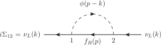
Figure 1: One-loop diagram for the $\Sigma_{12}$ element of the neutrino thermal self-energy in an $f\phi$ background.

Here we have defined

$$x=\beta k\cdot u-\alpha\,,$$ (2.9)

and

$$n_{F}(z)=\frac{1}{e^{z}+1}\,,$$ (2.10)

is the fermion distribution function, written in terms of a dummy variable $z$. For future reference we define here the corresponding function for the bosons,

$$n_{B}(z)=\frac{1}{e^{z}-1}\,.$$ (2.11)

2.2 Dispersion relation - damping term

The question we address here is how to determine the damping term in the dispersion relation, given the result for $\Sigma_{i}$. As already mentioned, the dispersion relation is determined by solving Eq. (2.3). Furthermore, the chirality of the neutrino interactions imply that $\Sigma_{eff}$ is of the form

$$\Sigma_{eff}=V\hbox to0.0pt{\hss/}L\,.$$ (2.12)

We consider now the determination of the dispersion relation for the case in which $V^{\mu}$ contains an absorptive part in addition to the dispersive part that we have considered in Ref. [13]. Therefore, here we assume that $V^{\mu}$ has a real and an imaginary part,

$$V^{\mu}=V^{\mu}_{r}+iV^{\mu}_{i}\,,$$ (2.13)

We should keep in mind that, in general, both $V^{\mu}_{r,i}$ are functions of $\omega$ and $\vec{\kappa}$, which will indicate by writing $V^{\mu}_{r,i}(\omega,\vec{\kappa})$ when needed.

We summarize the results as follows. Writing the neutrino and antineutrino dispersion relations in the form

$$\omega^{(\nu,\bar{\nu})}=\omega^{(\nu,\bar{\nu})}_{r}-\frac{i\gamma^{(\nu,\bar{\nu})}}{2}\,,$$ (2.14)

$\omega^{(\nu,\bar{\nu})}_{r}$ is given by

$$\omega^{(\nu,\bar{\nu})}_{r}=\kappa+V^{(\nu,\bar{\nu})}_{eff}$$ (2.15)

where $V^{(\nu,\bar{\nu})}_{eff}$ are the effective potentials

$$V^{(\nu)}_{eff} = n\cdot V_{r}(\kappa,\vec{\kappa})=V^{0}_{r}(\kappa,\vec{\kappa})-\hat{\kappa}\cdot\vec{V}_{r}(\kappa,\vec{\kappa})\,,$$

$$V^{(\bar{\nu})}_{eff} = -n\cdot V_{r}(-\kappa,-\vec{\kappa})=-V^{0}_{r}(-\kappa,-\vec{\kappa})+\hat{\kappa}\cdot\vec{V}_{r}(-\kappa,-\vec{\kappa})\,,$$ (2.16)

with

$$n^{\mu}=(1,\hat{\kappa})\,.$$ (2.17)

On the other hand, for the imaginary part we have

$$-\frac{\gamma^{(\nu)}(\vec{\kappa})}{2} = \frac{n\cdot V_{i}(\kappa,\vec{\kappa})}{1-n\cdot\left.\frac{\partial V_{r}(\omega,\vec{\kappa})}{\partial\omega}\right|_{\omega=\kappa}}\,,$$

$$-\frac{\gamma^{(\bar{\nu})}(\vec{\kappa})}{2} = \frac{n\cdot V_{i}(-\kappa,-\vec{\kappa})}{1-n\cdot\left.\frac{\partial V_{r}(\omega,-\vec{\kappa})}{\partial\omega}\right|_{\omega=-\kappa}}\,,$$ (2.18)

where $n^{\mu}$ is defined in Eq. (2.17). Eqs. (2.15) and (2.2), allow us to obtain the neutrino and antineutrino dispersion relation and damping from the self-energy. In those cases in which the correction due to the $n\cdot\partial V_{r}(\omega,\vec{\kappa})/\partial\omega$ in the denominator can be neglected, the formulas in Eq. (2.2) further simplify to

$$-\frac{\gamma^{(\nu)}(\vec{\kappa})}{2} = n\cdot V_{i}(\kappa,\vec{\kappa})\,,$$

$$-\frac{\gamma^{(\bar{\nu})}(\vec{\kappa})}{2} = n\cdot V_{i}(-\kappa,-\vec{\kappa})\,.$$ (2.19)

The formulas in Eq. (2.2) were used in Ref. [13] to calculate the real part of the neutrino dispersion relation in the $f\phi$ background. Eq. (2.2) are the ones we will use in the present work to calculate the damping terms in the dispersion relation.

These results are obtained as follows. From Eqs. (2.3) and (2.12), the dispersion relations must satisfy

$$(k-V)^{2}=0\,,$$ (2.20)

or

$$\omega-V^{0}=\pm\sqrt{(\vec{\kappa}-V)\cdot(\vec{\kappa}-\vec{V})}\,.$$ (2.21)

Remembering that $V^{\mu}$ is a function of $\omega$ and $\vec{\kappa}$, this is an implicit equation that determines the dispersion relations $\omega(\vec{\kappa})$. We consider the solution of Eq. (2.21) for the case in which $V^{\mu}$ is smaller than $\kappa$, so that we can treat the equation perturbatively.

Let us (re)consider first the real case ($V^{\mu}_{i}=0$). Denoting the solutions in this case by $\omega^{(\lambda)}_{r}$ ($\lambda=\pm$), they must satisfy

$$\omega^{(\lambda)}_{r}-V^{0}_{r}(\omega^{(\lambda)}_{r},\vec{\kappa}) = \lambda\sqrt{\left(\vec{\kappa}-\vec{V}_{r}(\omega^{(\lambda)}_{r},\vec{\kappa})\right)\cdot\left(\vec{\kappa}-\vec{V}_{r}(\omega^{(\lambda)}_{r},\vec{\kappa})\right)}$$ (2.22)

$$\simeq \lambda\left(\kappa-\hat{\kappa}\cdot\vec{V}_{r}(\omega^{(\lambda)}_{r},\vec{\kappa})\right)\,.$$

Thus, to the lowest order,

$$\omega^{(\pm)}_{r}(\vec{\kappa})=V^{0}_{r}(\pm\kappa,\vec{\kappa})\pm\left(\kappa-\hat{\kappa}\cdot\vec{V}_{r}(\pm\kappa,\vec{\kappa})\right)\,.$$ (2.23)

The neutrino and antineutrino dispersion relations are given by

$$\omega^{(\nu)}_{r} = \omega^{(+)}_{r}(\vec{\kappa})\,,$$

$$\omega^{(\bar{\nu})}_{r} = -\omega^{(-)}_{r}(-\vec{\kappa})\,,$$ (2.24)

which reduce to Eq. (2.15).

We now generalize this to the case with $V^{\mu}_{i}\not=0$. In analogy to Eq. (2.22), from Eq. (2.21) we obtain to first order

$$\omega^{(\lambda)}-V^{0}(\omega^{(\lambda)},\vec{\kappa})\simeq\lambda\left(\kappa-\hat{\kappa}\cdot\vec{V}(\omega^{(\lambda)},\vec{\kappa})\right)\,.$$ (2.25)

We seek the solution by writing

$$\omega^{(\lambda)}=\omega^{(\lambda)}_{r}+i\omega^{(\lambda)}_{i}\,,$$ (2.26)

and we work under the assumption that the imaginary parts are smaller than the real parts, in other words $\omega^{(\lambda)}_{i}\ll\omega^{(\lambda)}_{r}$. Therefore we write

$$V^{\mu}(\omega^{(\lambda)},\vec{\kappa}) \simeq V^{\mu}(\omega^{(\lambda)}_{r},\vec{\kappa})+i\omega^{(\lambda)}_{i}\left.\frac{\partial V^{\mu}(\omega,\vec{\kappa})}{\partial\omega}\right|_{\omega=\omega^{(\lambda)}_{r}}$$ (2.27)

$$\mbox{}\simeq V^{\mu}_{r}(\omega^{(\lambda)}_{r},\vec{\kappa})+iV^{\mu}_{i}(\omega^{(\lambda)}_{r},\vec{\kappa})+i\omega^{(\lambda)}_{i}\left.\frac{\partial V^{\mu}_{r}(\omega,\vec{\kappa})}{\partial\omega}\right|_{\omega=\omega^{(\lambda)}_{r}}\,,$$

neglecting terms of the second order in the imaginary parts.

Substituting Eq. (2.27) into Eq. (2.25), the real part yields Eq. (2.22), while the imaginary part, after some rearrangements, yields

$$\omega^{(\lambda)}_{i}(\vec{\kappa})=\frac{n^{(\lambda)}\cdot V_{i}(\omega^{(\lambda)}_{r},\vec{\kappa})}{1-n^{(\lambda)}\cdot\left.\frac{\partial V_{r}(\omega,\vec{\kappa})}{\partial\omega}\right|_{\omega=\omega^{(\lambda)}_{r}}}\,,$$ (2.28)

where we have defined

$$n^{(\lambda)\mu}=(1,\lambda\hat{\kappa})\,.$$ (2.29)

Eq. (2.28) can be simplified by approximating $\omega_{r}^{(\pm)}\simeq\pm\kappa$ in the evaluation of the right-hand side. Then, remembering that

$$\omega^{(\nu)}_{i}(\vec{\kappa}) = \omega^{(+)}_{i}(\vec{\kappa})$$

$$\omega^{(\bar{\nu})}_{i}(\vec{\kappa}) = \omega^{(-)}_{i}(-\vec{\kappa})\,,$$ (2.30)

and identifying the damping rate by

$$\omega^{(\nu,\bar{\nu})}_{i}=-\frac{\gamma^{(\nu,\bar{\nu})}}{2}\,,$$ (2.31)

we arrive at Eq. (2.2).

3 Damping term in an $f\phi$ background

3.1 Integral expressions for $\Sigma_{i}$ and $V^{\mu}_{i}$

The diagram in Fig. 1 gives the expression

$$-i\Sigma_{12}(k)=(i\lambda)(-i\lambda^{\ast})\int\frac{d^{4}p}{(2\pi)^{4}}i\Delta^{(\phi)}_{21}(q)RiS^{(f)}_{12}(p)L\,,$$ (3.1)

where

$$q=p-k\,.$$ (3.2)

The various components of the propagator matrices are

$$S^{(f)}_{12}(p) = 2\pi i\delta(p^{2}-m^{2}_{f})\left[\eta_{F}(p,\alpha_{f})-\theta(-p\cdot u)\right](p\hbox to0.0pt{\hss/}+m_{f})\,,$$

$$\Delta^{(\phi)}_{21}(q) = -2\pi i\delta(q^{2}-m^{2}_{\phi})\left[\eta_{B}(q,\alpha_{\phi})+\theta(q\cdot u)\right]\,,$$ (3.3)

where

$$\eta_{F}(p,\alpha_{f}) = \theta(p\cdot u)n_{F}(x_{f})+\theta(-p\cdot u)n_{F}(-x_{f})\,,$$

$$\eta_{B}(q,\alpha_{\phi}) = \theta(q\cdot u)n_{B}(x_{\phi})+\theta(-q\cdot u)n_{B}(-x_{\phi})\,,$$ (3.4)

with

$$x_{f} = \beta p\cdot u-\alpha_{f}\,,$$

$$x_{\phi} = \beta q\cdot u-\alpha_{\phi}\,$$ (3.5)

and $\theta$ is the step function. Further, $n_{F,B}$ are the fermion and boson distribution functions already defined in Eqs. (2.10) and (2.11). It is useful to recall that the parameters $\alpha_{f,\phi}$ and the corresponding one for the neutrinos, $\alpha$, must satisfy

$$\alpha+\alpha_{\phi}=\alpha_{f}\,,$$ (3.6)

by virtue of the $\bar{f}\nu\phi$ interaction. Therefore, together with momentum conservation, the following useful relation holds between $x_{f,\phi}$ and $x$,

$$x+x_{\phi}=x_{f}\,.$$ (3.7)

Then, using identities of the $n_{F,B}$ functions as well as Eq. (3.7), after some manipulations we can write

$$\Delta^{(\phi)}_{21}(q)S^{(f)}_{12}(p) = (2\pi)^{2}(p\hbox to0.0pt{\hss/}+m_{f})\delta(p^{2}-m^{2}_{f})\delta(q^{2}-m^{2}_{\phi})$$ (3.8)

$$\mbox{}\times n_{F}(x)\left(n_{B}(x_{\phi})+n_{F}(x_{f})\right)\epsilon(q\cdot u)\epsilon(p\cdot u)\,,$$

and then from Eq. (2.8)

$$\Sigma_{i} = -\frac{|\lambda|^{2}}{2}\int\frac{d^{4}p}{(2\pi)^{3}}\frac{d^{4}q}{(2\pi)^{3}}(2\pi)^{4}\delta^{(4)}(k+q-p)\delta(p^{2}-m^{2}_{f})\delta(q^{2}-m^{2}_{\phi})$$ (3.9)

$$\mbox{}\times\left(n_{B}(x_{\phi})+n_{F}(x_{f})\right)\epsilon(q\cdot u)\epsilon(p\cdot u)p\hbox to0.0pt{\hss/}L\,,$$

where $\epsilon(z)=\theta(z)-\theta(-z)$ with $\theta$ being the step function. In writing Eq. (3.9), only the term of $S^{(f)}_{12}$ proportional to $p\hbox to0.0pt{\hss/}$ contributes due to chirality, and we have inserted the factor $d^{4}q\,\delta^{(4)}(k+q-p)$ for convenience in the manipulations that follow.

The integrations over $p^{0}$ and $q^{0}$ can be carried out with the help of the $\delta$ functions, and with some change of variables,

$$\Sigma_{i} = -\frac{|\lambda|^{2}}{2}\int\frac{d^{3}p}{(2\pi)^{3}2E}\frac{d^{3}q}{(2\pi)^{3}2\Omega}(2\pi)^{4}\left\{\delta^{(4)}(k+q-p)(f_{\phi}+f_{f})\right.$$ (3.10)

$$\mbox{}+\delta^{(4)}(k+p-q)(f_{\bar{\phi}}+f_{\bar{f}})$$

$$\mbox{}+\delta^{(4)}(k-q-p)(1+f_{\bar{\phi}}-f_{f})$$

$$\mbox{}+\left.\delta^{(4)}(k+q+p)(1+f_{\phi}-f_{\bar{f}})\right\}p\hbox to0.0pt{\hss/}L\,,$$

where

$$E = \sqrt{\vec{p}^{\;2}+m^{2}_{f}}\,,$$

$$\Omega = \sqrt{\vec{q}^{\;2}+m^{2}_{\phi}}\,,$$ (3.11)

and

$$f_{f,\bar{f}} = \frac{1}{e^{\beta E\mp\alpha_{f}}+1}\,,$$

$$f_{\phi,\bar{\phi}} = \frac{1}{e^{\beta\Omega\mp\alpha_{\phi}}-1}\,.$$ (3.12)

Eq. (3.10) expresses the contributions to $\Sigma_{i}$ in terms of the transition probabilities for the various processes in which the neutrino may be annihilated or created,

$$\nu+\phi \leftrightarrow f$$

$$\nu+\bar{f} \leftrightarrow \bar{\phi}$$

$$\nu \leftrightarrow f+\bar{\phi}$$

$$\nu+\bar{f}+\phi \leftrightarrow 0\,.$$ (3.13)

This correspondence can be made more evident by rewriting the factors that contain the distribution functions, for example,

$$f_{\phi}+f_{f}=f_{\phi}(1-f_{f})+f_{f}(1+f_{\phi})\,,$$ (3.14)

and similarly with the other terms. The last two process listed in Eq. (3.1) are forbidden by the kinematics, assuming the vacuum dispersion relations for the particles and $m_{\nu}=0$. Therefore only the first two are viable. However, as will be discussed in detail below, the kinematic conditions under which they occur are different and therefore not both are possible at the same time. Thus, identifying $V^{\mu}_{i}$ by writing

$$\Sigma_{i}=RV\hbox to0.0pt{\hss/}_{i}L\,,$$ (3.15)

then

$$V^{\mu}_{i}(\omega,\vec{\kappa}) = -\frac{|\lambda|^{2}}{2}\int\frac{d^{3}p}{(2\pi)^{3}2E}\frac{d^{3}q}{(2\pi)^{3}2\Omega}(2\pi)^{4}\left\{\delta^{(4)}(k+q-p)(f_{\phi}+f_{f})\right.$$ (3.16)

$$\mbox{}+\left.\delta^{(4)}(k+p-q)(f_{\bar{\phi}}+f_{\bar{f}})\right\}p^{\mu}\,.$$

We have considered above the case in which the neutrino propagates in the presence of only one background, in this case composed of $f$ and $\phi$ particles. In this case the distribution functions that appear in Eq. (3.16) have the standard isotropic form given in Eq. (3.1). In a more general situation the medium can consist of various superimposed backgrounds, and in principle moving relative to each other with their own velocity four-vector $u^{\mu}_{s}$. For example, we can envisage a medium composed of a normal matter background, with a velocity four-vector $u^{\mu}$, and which we can take to be at rest, plus a stream background medium of $f$ and $\phi$ particles with some velocity four-vector $u^{\prime\,\mu}=(u^{\prime\,0},\vec{u}^{\,\prime})$. In such cases, the distribution functions that appear in Eq. (3.16) would have the form

$$f^{\prime}_{f,\bar{f}} = \frac{1}{e^{\beta p\cdot u^{\prime}\mp\alpha^{\prime}_{f}}+1}\,,$$

$$f^{\prime}_{\phi,\bar{\phi}} = \frac{1}{e^{\beta q\cdot u^{\prime}\mp\alpha^{\prime}_{\phi}}-1}\,,$$ (3.17)

which are not isotropic. In order to keep this possibility open, we consider the evaluation of Eq. (3.16) in the general case, without assuming isotropy of the distribution functions, and only consider the special isotropic case at the end.

3.2 Formula for the damping term

From Eq. (3.16),

$$V_{i}(\kappa,\vec{\kappa})\cdot n=-\left(\frac{|\lambda|^{2}}{16\pi^{2}\kappa}\right)\left[\Delta^{2}_{f\phi}(K^{\prime}_{\phi}+K^{\prime}_{f})+\Delta^{2}_{\phi f}(L^{\prime}_{\bar{\phi}}+L^{\prime}_{\bar{f}})\right]\,,$$ (3.18)

where

$$K^{\prime}_{\phi} = \int\frac{d^{3}p}{2E}\frac{d^{3}q}{2\Omega}\delta^{(4)}(k+q-p)f_{\phi}(\vec{q})\,,$$

$$K^{\prime}_{f} = \int\frac{d^{3}p}{2E}\frac{d^{3}q}{2\Omega}\delta^{(4)}(k+q-p)f_{f}(\vec{p})\,,$$

$$L^{\prime}_{\bar{\phi}} = \int\frac{d^{3}p}{2E}\frac{d^{3}q}{2\Omega}\delta^{(4)}(k+p-q)f_{\bar{\phi}}(\vec{q})\,,$$

$$L^{\prime}_{\bar{f}} = \int\frac{d^{3}p}{2E}\frac{d^{3}q}{2\Omega}\delta^{(4)}(k+p-q)f_{\bar{f}}(\vec{p})\,,$$ (3.19)

with

$$\Delta^{2}_{f\phi}=m^{2}_{f}-m^{2}_{\phi}\,,$$ (3.20)

and

$$\Delta^{2}_{\phi f}=m^{2}_{\phi}-m^{2}_{f}\,.$$ (3.21)

In obtaining Eq. (3.18) from Eq. (3.16) the factors $p\cdot n$ that would appear in the integrand can be reduced as follows using the momentum conservation delta functions. Consider the $K^{\prime}$ integrals, in which case

$$k+q=p\,.$$ (3.22)

Then

$$(p-k)^{2}=q^{2}\Rightarrow 2p\cdot k=m^{2}_{f}-m^{2}_{\phi}\,,$$ (3.23)

and using $k^{\mu}=\kappa n^{\mu}$,

$$p\cdot n=\frac{\Delta^{2}_{f\phi}}{2\kappa}\,.$$ (3.24)

Similarly, in the case of the $L^{\prime}$ integrals, the condition is $k+p=q$, and the corresponding relation is

$$p\cdot n=\frac{\Delta^{2}_{\phi f}}{2\kappa}\,.$$ (3.25)

This reduction is not possible in the case of the dispersive part of the potential $V_{r}(\kappa,\vec{\kappa})\cdot n$, therefore in that case the factor $p\cdot n$ (which can be expressed in the form $E(1-\vec{v}\cdot\hat{\kappa})$) remains in the integrand. We consider the $K^{\prime},L^{\prime}$ integrals one by one, using the results for the generic integral $I^{\prime}$ given in Appendix A. Although we are not indicating it explicitly, it should be remembered that in these integrals we are setting $\omega=\kappa$.

For $K^{\prime}_{\phi,f}$ the contributing process is $\nu+\phi\leftrightarrow f$. We then use the result given in Eq. (A.32) with the identification $1\rightarrow\phi,2\rightarrow f$. Thus, provided that

$$m_{f}>m_{\phi}\,,$$ (3.26)

then

$$K^{\prime}_{\phi} = \int\frac{d^{3}q}{2\Omega}\frac{1}{2\kappa|\vec{q}|}\delta\left(\hat{\kappa}\cdot\hat{q}-\cos\theta^{(I)}_{\phi}\right)\theta\left[\Omega-\Omega^{(I)}_{min}\right]f_{\phi}(\vec{q})\,,$$

$$K^{\prime}_{f} = \int\frac{d^{3}p}{2E}\frac{1}{2\kappa|\vec{p}|}\delta\left(\hat{\kappa}\cdot\hat{p}-\cos\theta^{(I)}_{f}\right)\theta\left[E-E^{(I)}_{min}\right]f_{f}(\vec{p})\,,$$ (3.27)

where

$$\cos\theta^{(I)}_{\phi} = \frac{2\kappa\Omega-\Delta^{2}_{f\phi}}{2\kappa|\vec{q}|}\,,$$

$$\cos\theta^{(I)}_{f} = \frac{2\kappa E-\Delta^{2}_{f\phi}}{2\kappa|\vec{p}|}\,,$$ (3.28)

and

$$\Omega^{(I)}_{min} = \frac{\Delta^{2}_{f\phi}}{4\kappa}+\frac{\kappa m^{2}_{\phi}}{\Delta^{2}_{f\phi}}\,,$$

$$E^{(I)}_{min} = \frac{\Delta^{2}_{f\phi}}{4\kappa}+\frac{\kappa m^{2}_{f}}{\Delta^{2}_{f\phi}}\,,$$ (3.29)

with $\Delta^{2}_{f\phi}$ given in Eq. (3.20). Similarly, for $L^{\prime}_{\bar{\phi},\bar{f}}$ the contributing process is $\nu+\bar{f}\leftrightarrow\bar{\phi}$, and we use Eq. (A.32) with the identifyication $1\rightarrow\bar{f},2\rightarrow\bar{\phi}$. Thus, provided

$$m_{\phi}>m_{f}\,,$$ (3.30)

we obtain in this case,

$$L^{\prime}_{\bar{\phi}} = \int\frac{d^{3}q}{2\Omega}\frac{1}{2\kappa|\vec{q}|}\delta\left(\hat{\kappa}\cdot\hat{q}-\cos\theta^{(II)}_{\phi}\right)\theta\left[\Omega-\Omega^{(II)}_{min}\right]f_{\bar{\phi}}(\vec{q})\,,$$

$$L^{\prime}_{\bar{f}} = \int\frac{d^{3}p}{2E}\frac{1}{2\kappa|\vec{p}|}\delta\left(\hat{k}\cdot\hat{p}-\cos\theta^{(II)}_{f}\right)\theta\left[E-E^{(II)}_{min}\right]f_{\bar{f}}(\vec{p})\,,$$ (3.31)

where

$$\cos\theta^{(II)}_{\phi} = \frac{2\kappa\Omega-\Delta^{2}_{\phi f}}{2\kappa|\vec{q}|}\,,$$

$$\cos\theta^{(II)}_{f} = \frac{2\kappa E-\Delta^{2}_{\phi f}}{2\kappa|\vec{p}|}\,,$$ (3.32)

and

$$\Omega^{(II)}_{min}=\frac{\Delta^{2}_{\phi f}}{4\kappa}+\frac{\kappa m^{2}_{\phi}}{\Delta^{2}_{\phi f}}\,,$$

$$E^{(II)}_{min}=\frac{\Delta^{2}_{\phi f}}{4\kappa}+\frac{\kappa m^{2}_{f}}{\Delta^{2}_{\phi f}}\,,$$ (3.33)

with $\Delta^{2}_{\phi f}$ in Eq. (3.21).

Using these results, from Eq. (2.2) the damping rate for the neutrino is then

$$\frac{\gamma^{(\nu)}(\vec{\kappa})}{2}=\frac{|\lambda|^{2}}{16\pi^{2}\kappa}\left\{\begin{array}[]{ll}\Delta^{2}_{f\phi}(K^{\prime}_{\phi}+K^{\prime}_{f})&(m_{f}>m_{\phi}),\;(\nu+\phi\leftrightarrow f)\\[12.0pt] \Delta^{2}_{\phi f}(L^{\prime}_{\bar{\phi}}+L^{\prime}_{\bar{f}})&(m_{\phi}>m_{f}),\;(\nu+\bar{f}\leftrightarrow\bar{\phi})\end{array}\right.$$ (3.34)

with $K^{\prime}_{f,\phi},L^{\prime}_{\bar{f},\bar{\phi}}$ given in Eqs. (3.2) and (3.2). We have indicated in parenthesis the kinematic condition on the masses and, for reference purposes, the contributing process. For the antineutrino the relevant quantity is $V_{i}(-\kappa,-\vec{\kappa})\cdot n$. From Eq. (3.16), in this case we obtain

$$V_{i}(-\kappa,-\vec{\kappa})\cdot n=-\left(\frac{|\lambda|^{2}}{16\pi^{2}\kappa}\right)\left[\Delta^{2}_{f\phi}(\bar{K}^{\prime}_{\phi}+\bar{K}^{\prime}_{f})+\Delta^{2}_{\phi f}(\bar{L}^{\prime}_{\bar{\phi}}+\bar{L}^{\prime}_{\bar{f}})\right]\,,$$ (3.35)

where $\bar{K}^{\prime}_{f,\phi},\bar{L}^{\prime}_{\bar{f},\bar{\phi}}$ are defined as $K^{\prime}_{f,\phi},L^{\prime}_{\bar{f},\bar{\phi}}$ in Eq. (3.2), but making the substitutions

$$f_{f}\leftrightarrow f_{\bar{f}}\,,\qquad f_{\phi}\leftrightarrow f_{\bar{\phi}}\,.$$ (3.36)

Correspondingly, the final formulas for $\bar{K}^{\prime}_{f,\phi},\bar{L}^{\prime}_{\bar{f},\bar{\phi}}$ can be obtained from Eqs. (3.2) and (3.2) by making the same substitutions. Thus, from Eq. (2.2), for the antineutrino

$$\frac{\gamma^{(\bar{\nu})}(\vec{\kappa})}{2}=\frac{|\lambda|^{2}}{16\pi^{2}\kappa}\left\{\begin{array}[]{ll}\Delta^{2}_{f\phi}(\bar{K}^{\prime}_{\phi}+\bar{K}^{\prime}_{f})&(m_{f}>m_{\phi}),\;(\bar{\nu}+\bar{\phi}\leftrightarrow\bar{f})\\[12.0pt] \Delta^{2}_{\phi f}(\bar{L}^{\prime}_{\bar{\phi}}+\bar{L}^{\prime}_{\bar{f}})&(m_{\phi}>m_{f}),\;(\bar{\nu}+f\leftrightarrow\phi)\end{array}\right.$$ (3.37)

3.3 Evaluation of the damping term for an isotropic $f\phi$ background

When the momentum distributions have the standard form the $K^{\prime},L^{\prime}$ integrals can be readily evaluated. The results can be read off the generic result given in Eq. (A.33) with the same identifications as made above, namely $1\rightarrow\phi,2\rightarrow f$ and $1\rightarrow\bar{f},2\rightarrow\bar{\phi}$ for the $K^{\prime}$ and $L^{\prime}$ integrals, respectively. Thus, using Eq. (A.33) in the manner we have indicated, we obtain from Eq. (3.34) the following result for the damping term, depending on whether $m_{f}>m_{\phi}$ or $m_{\phi}>m_{f}$,

$$\frac{\gamma^{(\nu)}(\kappa)}{2}=\frac{|\lambda|^{2}}{32\pi\kappa^{2}\beta}\left\{\begin{array}[]{ll}\Delta^{2}_{f\phi}\left[\log\left(1+e^{-\beta E^{(I)}_{min}+\alpha_{f}}\right)-\log\left(1-e^{-\beta\Omega^{(I)}_{min}+\alpha_{\phi}}\right)\right]&(m_{f}>m_{\phi})\\[12.0pt] \Delta^{2}_{\phi f}\left[\log\left(1+e^{-\beta E^{(II)}_{min}-\alpha_{f}}\right)-\log\left(1-e^{-\beta\Omega^{(II)}_{min}-\alpha_{\phi}}\right)\right]&(m_{\phi}>m_{f})\end{array}\right.$$ (3.38)

The corresponding formulas for $\frac{\gamma^{(\bar{\nu})}(\kappa)}{2}$ are obtained by making the substitutions

$$\alpha_{f,\phi}\rightarrow-\alpha_{f,\phi}\,,$$ (3.39)

in Eq. (3.38). In particular, if the background is particle-antiparticle symmetric, so that the chemical potentials $\alpha_{f,\phi}$ are zero, then $\gamma^{(\bar{\nu})}(\kappa)$ and $\gamma^{(\nu)}(\kappa)$ are equal, as expected on general grounds based on the $CPT$ symmetry of the background in that case.

4 Discussion

We illustrate some particular features of Eq. (3.38) by considering specific situations.

4.1 Degenerate $f$ background

For example, let us consider the case in which the scalar particle is so heavy that it is not present in the background. To be specific let us take $m_{\phi}\gg m_{f}$. In this example the contributing process is $\nu+\bar{f}\leftrightarrow\bar{\phi}$. Then from Eq. (3.38),

$$\frac{\gamma^{(\nu)}(\kappa)}{2}=\frac{|\lambda|^{2}m^{2}_{\phi}}{32\pi\kappa^{2}\beta}\log\left(1+e^{-\beta\epsilon^{(II)}_{min}-\alpha_{f}}\right)\,.$$ (4.1)

where, from Eq. (3.2), we have approximated

$$E^{(II)}_{min}\simeq\epsilon^{(II)}_{min}\equiv\frac{m^{2}_{\phi}}{4\kappa}+\frac{\kappa m^{2}_{f}}{m^{2}_{\phi}}$$ (4.2)

in the present case. Let us further assume that the $\bar{f}$ fermions form a completely degenerate gas and there are no $f$ fermions. Then setting

$$\alpha_{f}=-\beta E_{F}\,,$$ (4.3)

where $E_{F}$ is the Fermi energy, and taking the degenerate limit ($\beta\rightarrow\infty$),

$$\frac{\gamma^{(\nu)}(\kappa)}{2}=\frac{|\lambda|^{2}m^{2}_{\phi}}{32\pi\kappa^{2}}\left(E_{F}-\epsilon^{(II)}_{min}\right)\theta\left(E_{F}-\epsilon^{(II)}_{min}\right)\,,$$ (4.4)

while $\gamma^{(\bar{\nu})}(\kappa)=0$. The step function in Eq. (4.4) implies that $\gamma^{(\nu)}(\kappa)$ is non-zero if $\kappa$ lies in the range such that

$$\frac{1}{2}(E_{F}-p_{F})<\frac{\kappa m^{2}_{f}}{m^{2}_{\phi}}<\frac{1}{2}(E_{F}+p_{F})\,,$$ (4.5)

or it is zero otherwise On the other hand, if we assume that it is the $f$ fermions that form a completely degenerate gas and there are no $\bar{f}$ fermions, then we have $\gamma^{(\nu)}(\kappa)=0$ while $\gamma^{(\bar{\nu})}(\kappa)$ is given by a formula identical to Eq. (4.4), but in this case $E_{F}$ referring to the Fermi energy of the $f$ fermion gas and $\alpha_{f}=\beta E_{F}$.

4.2 Classical relativistic $f$ and $\bar{f}$ gas

In contrast, if we take a neutral ($\alpha_{f}=0$) gas of fermions, and assume that it can be considered in the classical regime then we obtain

$$\frac{\gamma^{(\nu)}(\kappa)}{2}=\frac{\gamma^{(\bar{\nu})}(\kappa)}{2}\simeq\frac{|\lambda|^{2}m^{2}_{\phi}}{32\pi\kappa^{2}\beta}e^{-\beta\epsilon^{(II)}_{min}}\,,$$ (4.11)

where $\epsilon^{(II)}_{min}$ has been defined in Eq. (4.2). In this case, the damping has a maximum value at the value of $\kappa$ determined by the condition

$$\frac{d\epsilon^{(II)}_{min}}{d\kappa}=-\frac{2}{\beta\kappa}\,,$$ (4.12)

where

$$\frac{d\epsilon^{(II)}_{min}}{d\kappa}=-\frac{m^{2}_{\phi}}{4\kappa^{2}}+\frac{m^{2}_{f}}{m^{2}_{\phi}}\,.$$ (4.13)

As an example, suppose that the conditions, to be determined below, are such that the term $m^{2}_{f}/m^{2}_{\phi}$ in Eq. (4.12) can be neglected. This gives

$$\kappa=\frac{\beta m^{2}_{\phi}}{8}\,.$$ (4.14)

Notice that for this value of $\kappa$,

$$\frac{2}{\beta\kappa}=\frac{m^{2}_{\phi}}{4\kappa^{2}}=\frac{16}{\beta^{2}m^{2}_{\phi}}\,,$$ (4.15)

so that indeed the $m^{2}_{f}/m^{2}_{\phi}$ term can be neglected if the $f,\bar{f}$ gas is ultra-relativistic ($\beta m_{f}\ll 1$). Consequently the maximum value of the damping is

$$\frac{\gamma^{(\nu)}}{2}=\frac{\gamma^{(\bar{\nu})}}{2}=\frac{2|\lambda|^{2}}{\pi m^{2}_{\phi}\beta^{3}}e^{-2}\,,$$ (4.16)

which occurs at the value of $\kappa$ given in Eq. (4.14). For other values of $\kappa$ the damping drops exponentially.

4.3 Classical relativistic $\phi$ background

We now consider the opposite case, namely $m_{f}>m_{\phi}$ and assume that the conditions are such that there are no fermions in the background. In addition we assume that the scalar $\phi$ is its own antiparticle and therefore $\alpha_{\phi}=0$. In this case the contributing process is $\nu+\phi\leftrightarrow f$. From Eq. (3.38),

$$\frac{\gamma^{(\nu)}(\kappa)}{2}=\frac{\gamma^{(\bar{\nu})}(\kappa)}{2} = -\frac{|\lambda|^{2}m^{2}_{f}}{32\pi\kappa^{2}\beta}\log\left(1-e^{-\beta\omega^{(I)}_{min}}\right)$$ (4.17)

$$= \frac{|\lambda|^{2}m^{2}_{f}}{32\pi\kappa^{2}\beta}e^{-\beta\omega^{(I)}_{min}}\,,$$

where in the last line we have approximated

$$\Omega^{(I)}_{min}\simeq\omega^{(I)}_{min}\equiv\frac{m^{2}_{f}}{4\kappa}+\frac{\kappa m^{2}_{\phi}}{m^{2}_{f}}\,,$$ (4.18)

and assumed that the $\phi$ background can be treated within the classical approximation. Furthermore, if we consider a relativistic $\phi$ gas, then by carrying out steps similar to those leading to Eq. (4.16), we obtain in this case the maximum value of the damping

$$\frac{\gamma^{(\nu)}}{2}=\frac{\gamma^{(\bar{\nu})}}{2}=\frac{2|\lambda|^{2}}{\pi m^{2}_{f}\beta^{3}}e^{-2}\,,$$ (4.19)

at the momentum

$$\kappa=\frac{\beta m^{2}_{f}}{8}\,.$$ (4.20)

5 Damping term in a $\nu\phi$ background

The results we have obtained in the previous sections can be adapted to the case of a neutrino propagating in a neutrino and scalar background. For example, we can assume that a sterile ($\nu_{s}$) and an active neutrino have an interaction of the form

$$L_{int}=\lambda^{(\nu\nu_{s}\phi)}{\bar{\nu}}^{c}_{Rs}{\nu}_{L}\phi+h.c.$$ (5.1)

and consider the cases of either $\nu$ or $\nu_{s}$ propagating in a background of the other plus $\phi$. With the appropriate identifications the formulas we have presented can be used in either case, with the provision that the propagating neutrino is considered to be massless.

In the rest of this section we consider another case, namely the damping effects in a neutrino and scalar background, due to the diagonal interaction given in Eq. (1.1). In the relevant diagram for this case, shown in Fig. 2, the internal fermion that corresponds to the $f_{R}$ fermion line in Fig. 1 is the antineutrino $\nu^{c}_{R}$.

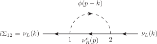
Figure 2: One-loop diagram for the $\Sigma_{12}$ element of the neutrino thermal self-energy in a $\nu\phi$ background.

Thus, the formulas obtained in Section 3 and 4 can be adapted to this case by identifying $f,\bar{f}\rightarrow\bar{\nu},\nu$ in the labels of the various physical quantities that refer to the background particles, such as the chemical potentials. We restrict ourselves here to the case of isotropic $\nu$ and $\phi$ backgrounds, in which case we can use the formulas given in Eq. (3.38) as the starting point. Since the background neutrino is the same as the initial neutrino, which have taken to be massless, we use the formula for $m_{\phi}>m_{f}$ (which corresponds to the process $\nu+\nu\leftrightarrow\bar{\phi}$). Therefore

$$\frac{\gamma^{(\nu)}(\kappa)}{2}=\frac{|\lambda^{(\nu\nu\phi)}|^{2}}{32\pi\kappa^{2}\beta}\Delta^{2}_{\phi\nu}\left[\log\left(1+e^{-\beta E^{(II)}_{min}+\alpha_{\nu}}\right)-\log\left(1-e^{-\beta\Omega^{(II)}_{min}-\alpha_{\phi}}\right)\right]\,,$$ (5.2)

where we have set $\alpha_{f}\rightarrow\alpha_{\bar{\nu}}=-\alpha_{\nu}$, as we have indicated above. Furthermore, borrowing from Eq. (3.2) and remembering that in this case $m_{\nu}\rightarrow 0$,

$$\Omega^{(II)}_{min} = \kappa+\frac{m^{2}_{\phi}}{4\kappa}\,,$$

$$E^{(II)}_{min} = \frac{m^{2}_{\phi}}{4\kappa}\,.$$ (5.3)

The corresponding formula for $\gamma^{(\bar{\nu})}(\kappa)$ is given by making the substitutions

$$\alpha_{\nu}\rightarrow-\alpha_{\nu},\;\alpha_{\phi}\rightarrow-\alpha_{\phi}\,,$$ (5.4)

in Eq. (5.2).

The formula in Eq. (5.2) and the corresponding one for $\gamma^{(\bar{\nu})}(\kappa)$ can be used to study different cases, for example, different conditions of the background gases, that can be useful in specific situations. For illustrative purposes let us consider the particular case in which the background density of the $\phi$ particles can be neglected. Assuming further that the neutrino gas can be treated in the classical regime, then we can use Eq. (4.16) and obtain

$$\frac{\gamma^{(\nu)}}{2}=\frac{\gamma^{(\bar{\nu})}}{2}=\frac{2|\lambda^{(\nu\nu\phi)}|^{2}T^{3}_{\nu}}{\pi m^{2}_{\phi}}e^{-2}\,,$$ (5.5)

where we are denoting by $T_{\nu}$ the temperature of the neutrino gas. Here we are assuming that the neutrino chemical potential is sufficiently small that we can use the damping formula with $\alpha_{\nu}\sim 0$. In order to assess the possible relative importance of the damping effects in this case, we recall from Ref. [13] the following result for the real part of the dispersion relation for this same example case,

$$\omega^{(\nu,\bar{\nu})}_{r}(\vec{\kappa})=\kappa+V^{(\nu,\bar{\nu})}_{eff}(\vec{\kappa})\,,$$ (5.6)

where

$$V^{(\nu,\bar{\nu})}_{eff}(\vec{\kappa})=\pm\left(2\sqrt{2}G_{F}-\frac{|\lambda^{(\nu\nu\phi)}|^{2}}{2m^{2}_{\phi}}\right)(n_{\nu}-n_{\bar{\nu}})+O(1/m^{4}_{\phi})\,.$$ (5.7)

Therefore, the importance of the damping term depends on the magnitude of

$$\frac{|\lambda^{(\nu\nu\phi)}|^{2}T^{3}_{\nu}}{m^{2}_{\phi}}\,,$$ (5.8)

relative to

$$\frac{g^{2}}{m^{2}_{Z}}(n_{\nu}-n_{\bar{\nu}})\,,$$ (5.9)

and

$$\frac{|\lambda^{(\nu\nu\phi)}|^{2}}{m^{2}_{\phi}}(n_{\nu}-n_{\bar{\nu}})\,.$$ (5.10)

As pointed out in Ref. [13], requiring that the $\phi$ exchange contribution to $\omega^{(\nu,\bar{\nu})}_{r}(\vec{\kappa})$ be smaller than the standard $Z$-exchange contribution implies that

$$m_{\phi}>\frac{|\lambda^{(\nu\nu\phi)}|}{g}m_{Z}\,.$$ (5.11)

For example, if $|\lambda^{(\nu\nu\phi)}|\sim O(1)$, this would imply that $m_{\phi}$ must be larger than $\sim 3m_{Z}$. On the other hand, in order to have $m_{\phi}\sim O(GeV)$, a small coupling $|\lambda^{(\nu\nu\phi)}|\sim 10^{-2}-10^{-3}$ would be required.

However, as this example shows, the damping term can be as large as the $\nu\phi$ contribution to $V^{(\nu,\bar{\nu})}_{eff}$. In fact, the relative importance of the damping term may be more significant if the neutrino-antineutrino asymmetry in the background is small, because the $O(1/m^{2}_{Z})$ and $O(1/m^{2}_{\phi})$ contributions to $V^{(\nu,\bar{\nu})}_{eff}$ are suppressed in that case, while the damping term is not.

6 Conclusions

The neutrino interactions with scalar particles via couplings of the form $\lambda^{(\nu\nu\phi)}\bar{\nu}^{c}_{R}\nu_{L}\phi$ can produce nonstandard contributions to the neutrino index of refraction and effective potential when the neutrino propagates in a neutrino background. This occurs in the environment of a supernova, and in the Early Universe hot plasma before neutrino decoupling. Motivated by this, we had previously[13] considered a simple model in which the neutrino interacts with a scalar and a fermion background with a coupling of the form $\lambda\bar{f}_{R}\nu_{L}\phi$. In Ref. [13] we focused exclusively on the calculation of the real part of the dispersion relation and effective potential for a neutrino propagating in a thermal background of those particles.

In the present work we have complemented those calculations by considering the damping terms in the neutrino effective potential and index of refraction. The damping terms arise as a consequence ofo processes such as $\nu+\phi\leftrightarrow f$ and $\nu+\bar{f}\leftrightarrow\bar{\phi}$ that occur when the neutrino propagates in the $f\phi$ background, depending on the kinematics conditions. Specifically, we calculated the imaginary part of the neutrino self-energy, from which the damping terms in the neutrino effective potential and dispersion relations were determined. The formulas for the case of the neutrino and scalar background, were then obtained as the special case in which $f_{R}\rightarrow\nu^{c}_{R}$.

The results are useful in the context of Dark Matter-neutrino interaction models in which the scalar and/or fermion constitute the dark-matter. They are also applicable to the situations mentioned above in which the fermion background is a neutrino background, including, for example, a sterile neutrino interacting with a neutrino background or the other way around. We obtained the expressions for the damping terms in the neutrino effective potential that can be applied to different situations and background conditions. For definiteness, we obtained explicit formulas for the damping terms in the case that the background particle momentum distributions have the standard isotropic form, but for generality and in order to present the results in a way that can be useful to the situations described and others not considered here, the generalization to the case of an anisotropic background was mentioned.

As specific application we considered the case in which the scalar is sufficiently heavy such that their distribution function can be neglected, and for definiteness the neutrino gas can be treated in the classical regime. As that particular example showed, the damping term can be as large as the contribution to effective potential. Moreover, the importance of the damping term becomes more significant when the neutrino-antineutrino asymmetry in the background is small, because the $O(1/m^{2}_{Z})$ and $O(1/m^{2}_{\phi})$ contributions to the effective potential are proportional to the neutrino-antineutrino asymmetry and therefore are suppressed in that case, while the damping term is not.

Despite the simplification and idealization we have made by considering only the diagonal scalar-neutrino coupling, the formulas and results we have presented can serve as a guide when considering more realistic or complicated situations, such as those involving more than one scalar particle or off-diagonal neutrino couplings, and to determine whether the damping effects are significant and must be considered or if they are small and can be neglected. For example, with off-diagonal neutrino couplings one neutrino can decay into another neutrino and a $\phi$ scalar (the third process type listed in Eq. (3.1). The corresponding contribution to the damping can be calculated in a manner similar to the calculations we have presented.

The work of S. S. is partially supported by DGAPA-UNAM (Mexico) Project No. IN103019.

Appendix A Evaluation of integrals

Here we derive the results quoted in Eqs. (3.2) and (3.2). Since the integrals involved have the generic form

$$I^{\prime}(\omega,\vec{\kappa})\equiv\int\frac{d^{3}p_{1}}{2E_{1}}\frac{d^{3}p_{2}}{2E_{2}}\delta^{(4)}(k+p_{1}-p_{2})F(\vec{p}_{1},\vec{p}_{2})\,,$$ (A.1)

we focus our attention for the moment on this kind of integral. We set

$$\omega=\kappa\,,$$ (A.2)

from the beginning since this is the appropriate limit for our purposes. Rewriting it as

$$I^{\prime}(\kappa,\vec{\kappa})=\int\frac{d^{3}p_{1}}{2E_{1}}d^{4}p_{2}\delta(p^{2}_{2}-m^{2}_{2})\theta(p^{0}_{2})\delta^{(4)}(k+p_{1}-p_{2})F(\vec{p}_{1},\vec{p}_{2})\,,$$ (A.3)

and doing the integral over $p_{2}$ first, we set

$$p_{2}=p_{1}+k\,,$$ (A.4)

and thus

$$I^{\prime}(\kappa,\vec{\kappa}) = \int\frac{d^{3}p_{1}}{2E_{1}}\delta[(k+p_{1})^{2}-m^{2}_{2}]\theta(\kappa+E_{1})F(\vec{p}_{1},\vec{p}_{1}+\vec{\kappa})$$ (A.5)

$$= \int\frac{d^{3}p_{1}}{2E_{1}}\left(\frac{1}{2\kappa|\vec{p}_{1}|}\right)F(\vec{p}_{1},\vec{p}_{1}+\vec{\kappa})\delta(\hat{\kappa}\cdot\hat{p}_{1}-\cos\theta_{1})\theta(\kappa+E_{1})\,,$$

where

$$\cos\theta_{1}\equiv\frac{2\kappa E_{1}-\Delta^{2}_{21}}{2\kappa p_{1}}\,,$$ (A.6)

with

$$\Delta^{2}_{21}=m^{2}_{2}-m^{2}_{1}\,.$$ (A.7)

$\cos\theta_{1}$ must satisfy

$$-1\leq\cos\theta_{1}\leq 1\,,$$ (A.8)

which requires

$$\Delta^{2}_{21}>0\,,$$ (A.9)

and also determines the $E_{1}$ limits of integration that we denote by $(E_{1})_{min}$ and $(E_{1})_{max}$. From the fact that $\vec{p}_{2}=\vec{\kappa}+\vec{p}_{1}$ together with Eq. (A.6) it follows that

$$\hat{\kappa}\cdot\hat{p}_{2}=\cos\theta_{2}\equiv\frac{2\kappa E_{2}-\Delta^{2}_{21}}{2\kappa p_{2}}\,,$$ (A.10)

where

$$E_{2}=E_{1}+\kappa\,.$$ (A.11)

In particular,

$$(E_{2})_{min,max}=(E_{1})_{min,max}+\kappa\,.$$ (A.12)

To find the limits implied by Eq. (A.6) we solve that relation for $E_{1},p_{1}$ as functions of $\cos\theta_{1}$. We rewrite it as

$$E_{1}=xp_{1}+\xi m_{1}\,,$$ (A.13)

where

$$x = \cos\theta_{1}\,,$$

$$\xi = \frac{\Delta^{2}_{21}}{2\kappa m_{1}}\,.$$ (A.14)

Then, putting $E_{1}=\sqrt{p^{2}_{1}+m^{2}_{1}}$ and solving Eq. (A.13) for $p_{1}$ yields

$$p_{1}=\frac{m_{1}}{y^{2}}\left\{x\xi\pm\sqrt{\xi^{2}-y^{2}}\right\}\,,$$ (A.15)

where

$$y=\sqrt{1-x^{2}}=\sin\theta_{1}\,,$$ (A.16)

and then

$$E_{1}=\frac{m_{1}}{y^{2}}\left\{\xi\pm x\sqrt{\xi^{2}-y^{2}}\right\}\,.$$ (A.17)

These solutions for $E_{1},p_{1}$ of course satisfy $E^{2}_{1}=p^{2}_{1}+m^{2}_{1}$, but we must be sure that they satisfy

$$E_{1},p_{1}>0\,,$$ (A.18)

as well. There are two possibilities.

Case I: $\xi>1\qquad(\kappa<\frac{\Delta^{2}_{21}}{2m_{1}})$

In this case we have

$$\sqrt{\xi^{2}-y^{2}}>x\xi\,,$$ (A.19)

and therefore the solution with the negative sign is not valid. Therefore in this case the only solution is

$$p_{1} = \frac{m_{1}}{y^{2}}\left\{x\xi+\sqrt{\xi^{2}-y^{2}}\right\}\,,$$

$$E_{1} = \frac{m_{1}}{y^{2}}\left\{\xi+x\sqrt{\xi^{2}-y^{2}}\right\}\,.$$ (A.20)

Case II: $\xi<1\qquad(\kappa>\frac{\Delta^{2}_{21}}{2m_{1}})$

In this case the factor $\sqrt{\xi^{2}-y^{2}}$ implies that there is a maximum value of $y$,

$$y_{max}=\xi\,,$$ (A.21)

so that

$$\sqrt{\xi^{2}-y^{2}}<x\xi\,,$$ (A.22)

which in turn implies that the solution with the minus sign is also allowed. Thus,

$$p^{(\pm)}_{1} = \frac{m_{1}}{y^{2}}\left\{x\xi\pm\sqrt{\xi^{2}-y^{2}}\right\}\,,$$

$$E^{(\pm)}_{1} = \frac{m_{1}}{y^{2}}\left\{\xi\pm x\sqrt{\xi^{2}-y^{2}}\right\}\,,$$ (A.23)

where $p_{1}>0\Rightarrow x>0$.

In either case, for $\cos\theta\rightarrow 1$ (which implies $y\rightarrow 0$) we have

$$(E_{1})_{max}=\left.E_{1}\right|_{x\rightarrow 1}=\infty\,.$$ (A.24)

On the other hand, $(E_{1})_{min}$ is given by $\left.E_{1}\right|_{x\rightarrow-1}$ in Case I, or $\left.E^{(-)}_{1}\right|_{x\rightarrow 1}$ in Case II. In either case,

$$(E_{1})_{min} = \left\{\frac{m_{1}}{y^{2}}\left[\xi-\left(1-\frac{y^{2}}{2}\right)\left(\xi-\frac{y^{2}}{2\xi}\right)\right]\right\}_{y\rightarrow 0}$$ (A.25)

$$= m_{1}\left[\frac{\xi}{2}+\frac{1}{2\xi}\right]$$

$$= \frac{\Delta^{2}_{21}}{4\kappa}+\frac{\kappa m^{2}_{1}}{\Delta^{2}_{21}}\,.$$

From Eq. (A.12),

$$(E_{2})_{min}=\frac{\Delta^{2}_{21}}{4\kappa}+\frac{\kappa m^{2}_{2}}{\Delta^{2}_{21}}\,.$$ (A.26)

We can summarize the results as follows. The kinematic conditions require that

$$m_{2}>m_{1}\,,$$ (A.27)

and the integration over $p_{1}$ is restricted by the condition

$$E_{1}\geq(E_{1})_{min}\,,$$ (A.28)

where $(E_{1})_{min}$ is given in Eq. (A.25). Then $I^{\prime}(\kappa,\vec{\kappa})$ can be expressed in the form

$$I^{\prime}(\kappa,\vec{\kappa})=\int\frac{d^{3}p_{1}}{2E_{1}}\left(\frac{1}{2\kappa|\vec{p}_{1}|}\right)\delta(\hat{\kappa}\cdot\hat{p}_{1}-\cos\theta_{1})\theta\left[E_{1}-(E_{1})_{min}\right]F(\vec{p}_{1},\vec{p}_{1}+\vec{\kappa})\qquad\mbox{(Form-1)}\,,$$ (A.29)

to which we refer as the Form-1. It can be expressed in the following equivalent form by carrying the integral over $p_{1}$ first,

$$I^{\prime}(\kappa,\vec{\kappa})=\int\frac{d^{3}p_{2}}{2E_{2}}\left(\frac{1}{2\kappa|\vec{p}_{2}|}\right)\delta(\hat{\kappa}\cdot\hat{p}_{2}-\cos\theta_{2})\theta\left[E_{2}-(E_{2})_{min}\right]F(\vec{p}_{2}-\vec{\kappa},\vec{p}_{2})\qquad\mbox{(Form-2)}\,,$$ (A.30)

where $\cos\theta_{2}$ and $(E_{2})_{min}$ are given in Eqs. (A.10) and (A.26), respectively. We refer to Eq. (A.30) as the Form-2. It then follows that if we define the integrals

$$I^{\prime}_{a}(\omega,\vec{\kappa})\equiv\int\frac{d^{3}p_{1}}{2E_{1}}\frac{d^{3}p_{2}}{2E_{2}}\delta^{(4)}(k+p_{1}-p_{2})f_{a}(p_{a})\qquad(a=1,2)\,,$$ (A.31)

then, using Eqs. (A.29) and (A.30) for $a=1,2$, respectively, we get

$$I^{\prime}_{a}(\kappa,\vec{\kappa})=\int\frac{d^{3}p_{a}}{2E_{a}}\left(\frac{1}{2\kappa|\vec{p}_{a}|}\right)\delta(\hat{\kappa}\cdot\hat{p}_{a}-\cos\theta_{a})\theta\left[E_{a}-(E_{a})_{min}\right]f_{a}(\vec{p}_{a})\,.$$ (A.32)

In the case that the momentum distributions have the standard isotropic form [e.g., Eq. (3.1)], the expression for $I^{\prime}_{a}(\kappa,\vec{\kappa})$ in Eq. (A.32) reduces to

$$I^{\prime}_{a}(\kappa,\vec{\kappa})=\frac{\pi}{2\kappa}I_{a}\,,$$ (A.33)

where $I_{a}$ is the elementary integral

$$I_{a}=\int^{\infty}_{(E_{a})_{min}}dE_{a}\,f_{a}(E_{a})=\left\{\begin{array}[]{ll}\frac{1}{\beta}\log\left[1+e^{-\beta(E_{a})_{min}+\alpha_{a}}\right]&(F)\\[12.0pt] -\frac{1}{\beta}\log\left[1-e^{-\beta(E_{a})_{min}+\alpha_{a}}\right]&(B)\end{array}\right.$$ (A.34)

where the labels $F$ and $B$ stand for either the fermion or boson distribution function, respectively. Eq. (A.32), and its counterpart Eq. (A.33) in the isotropic case, are the formulas we have used in the text.

For easy reference, we summarize here the following formulas that enter in Eqs. (A.29), (A.30) and (A.32),

$$(E_{1})_{min} = \frac{\Delta^{2}_{21}}{4\kappa}+\frac{\kappa m^{2}_{1}}{\Delta^{2}_{21}}\,,$$

$$\cos\theta_{1} = \frac{2\kappa E_{1}-\Delta^{2}_{21}}{2\kappa|\vec{p}_{1}|}\,,$$

$$(E_{2})_{min} = \frac{\Delta^{2}_{21}}{4\kappa}+\frac{\kappa m^{2}_{2}}{\Delta^{2}_{21}}\,,$$

$$\cos\theta_{2} = \frac{2\kappa E_{2}-\Delta^{2}_{21}}{2\kappa|\vec{p}_{2}|}\,,$$

$$\Delta^{2}_{21} \equiv m^{2}_{2}-m^{2}_{1}\,.$$ (A.35)

References

- [1] J. M. Berryman, A. De Gouvea, K. J. Kelly and Y. Zhang, Lepton-Number-Charged Scalars and Neutrino Beamstrahlung, Phys. Rev. D 97, 075030 (2018) [arxiv:1802.00009].
- [2] Y. Farzan, M. Lindner, W. Rodejohann and X. J. Xu, Probing neutrino coupling to a light scalar with coherent neutrino scattering, JHEP 1805, 066 (2018) [arxiv:1802.05171].
- [3] G. J. Stephenson Jr. and J. T. Goldman, Observable consequences of a scalar boson coupled only to neutrinos, [hep-ph/9309308].
- [4] C. Boehm, A. Olivares-Del Campo, S. Palomares-Ruiz and S. Pascoli, Phenomenology of a Neutrino-DM Coupling: The Scalar Case, [arxiv:1705.03692].
- [5] L. Heurtier and Y. Zhang, Supernova Constraints on Massive (Pseudo)Scalar Coupling to Neutrinos, JCAP 1702, 042 (2017) [arxiv:1609.05882].
- [6] R. F. Sawyer, Bulk viscosity of a gas of neutrinos and coupled scalar particles in the era of recombination, Phys. Rev. D 74, 043527 (2006) [arxiv:astro-ph/0601525].
- [7] P. S. Pasquini and O. L. G. Peres, Bounds on Neutrino-Scalar Yukawa Coupling, Phys. Rev. D 93, 053007 (2016) [arxiv:1511.01811]. Errata: Phys. Rev. D 93, 079902 (2016)
- [8] S. F. Ge, M. Lindner and W. Rodejohann, Atmospheric Trident Production for Probing New Physics, Phys. Lett. B 772, 164 (2017) [arxiv:1702.02617].
- [9] V. Brdar, J. Kopp, J. Liu, P. Prass and X. P. Wang, Fuzzy dark matter and nonstandard neutrino interactions, Phys. Rev. D 97, 043001 (2018) [arxiv:1705.09455].
- [10] T. Ohlsson, Status of non-standard neutrino interactions, Rept. Prog. Phys. 76, 044201 (2013) [arxiv:1209.2710].
- [11] S. Antusch, J. P. Baumann and E. Fernandez-Martinez, Non-Standard Neutrino Interactions with Matter from Physics Beyond the Standard Model, Nucl. Phys. B 810, 369 (2009) [arxiv:0807.1003].
- [12] M. G. Aartsen et al. (IceCube Collaboration), Search for Nonstandard Neutrino Interactions with IceCube DeepCore, Phys. Rev. D 97, 072009 (2018) [arxiv:1709.07079].
- [13] J. F. Nieves and S. Sahu, Neutrino effective potential in a fermion and scalar background, Phys. Rev. D 98, 063003 (2018) [arxiv:1808.01629].
- [14] H. Duan, G. M. Fuller and Y. Z. Qian, Collective Neutrino Oscillations, Ann. Rev. Nucl. Part. Sci. 60, 569 (2010) [arxiv:1001.2799].
- [15] S. Chakraborty, R. Hansen, I. Izaguirre and G. Raffelt, Collective neutrino flavor conversion: Recent developments, Nucl. Phys. B 908, 366 (2016) [arxiv:1602.02766].
- [16] Y. Y. Y. Wong, Analytical treatment of neutrino asymmetry equilibration from flavor oscillations in the early universe, Phys. Rev. D 66, 025015 (2002) [arxiv:hep-ph/0203180].
- [17] G. Mangano, G. Miele, S. Pastor, T. Pinto, O. Pisanti and P. D. Serpico, Effects of non-standard neutrino-electron interactions on relic neutrino decoupling, Nucl. Phys. B 756, 100 (2006) [arxiv:hep-ph/0607267].
- [18] R. Primulando and P. Uttayarat, Dark Matter-Neutrino Interaction in Light of Collider and Neutrino Telescope Data, JHEP 1806, 026 (2018) [arxiv:1710.08567].
- [19] T. Franarin, M. Fairbairn and J. H. Davis, JUNO Sensitivity to Resonant Absorption of Galactic Supernova Neutrinos by Dark Matter, [arxiv:1806.05015].
- [20] G. Mangano, A. Melchiorri, P. Serra, A. Cooray and M. Kamionkowski, Cosmological bounds on dark matter-neutrino interactions, Phys. Rev. D 74, 043517 (2006) [arxiv:astro-ph/0606190].
- [21] T. Binder, L. Covi, A. Kamada, H. Murayama, T. Takahashi and N. Yoshida, Matter Power Spectrum in Hidden Neutrino Interacting Dark Matter Models: A Closer Look at the Collision Term, JCAP 1611, 043 (2016) [arxiv:1602.07624].
- [22] A. Olivares-Del Campo, C. Bœhm, S. Palomares-Ruiz and S. Pascoli, Dark matter-neutrino interactions through the lens of their cosmological implications, Phys. Rev. D 97, 075039 (2018) [arxiv:1711.05283].
- [23] T. Brune and H. Päs, Majoron Dark Matter and Constraints on the Majoron-Neutrino Coupling, [arxiv:1808.08158].
- [24] Xiaoyong Chu, Basudeb Dasgupta, Mona Dentler, Joachim Kopp, Ninetta Saviano, Sterile Neutrinos with Secret Interactions - Cosmological Discord?, [arxiv1806.10629] and references therein.
- [25] J. C. D’Olivo, J. F. Nieves, Damping rate of a fermion in a medium, Phys. Rev. D 52, 2987 (1995) [arxiv:hep-ph/9309225].