SIGNet: Semantic Instance Aided Unsupervised 3D Geometry Perception

Yue Meng¹ Yongxi Lu¹ Aman Raj¹ Samuel Sunarjo¹ Rui Guo²
Tara Javidi¹ Gaurav Bansal² Dinesh Bharadia¹

¹UC San Diego ²Toyota InfoTechnology Center
{yum107, yol070, amraj, ssunarjo, tjavidi, dineshb}@ucsd.edu
rguo@us.toyota-itc.com gauravbs@gmail.com

Abstract

Unsupervised learning for geometric perception (depth, optical flow, etc.) is of great interest to autonomous systems. Recent works on unsupervised learning have made considerable progress on perceiving geometry; however, they usually ignore the coherence of objects and perform poorly under scenarios with dark and noisy environments. In contrast, supervised learning algorithms, which are robust, require large labeled geometric dataset. This paper introduces SIGNet, a novel framework that provides robust geometry perception without requiring geometrically informative labels. Specifically, SIGNet integrates semantic information to make depth and flow predictions consistent with objects and robust to low lighting conditions. SIGNet is shown to improve upon the state-of-the-art unsupervised learning for depth prediction by 30% (in squared relative error). In particular, SIGNet improves the dynamic object class performance by 39% in depth prediction and 29% in flow prediction. Our code will be made available at https://github.com/mengyuest/SIGNet

1 Introduction

Visual perception of 3D scene geometry using a monocular camera is a fundamental problem with numerous applications, like autonomous driving and space exploration. We focus on the ability to infer accurate geometry (depth and flow) of static and moving objects in a 3D scene. Supervised deep learning models have been proposed for geometry predictions, yielding “robust” and favorable results against the traditional approaches (SfM) [38, 39, 10, 2, 1, 26]. However, supervised models require a dataset labeled with geometrically informative annotations, which is extremely challenging as the collection of geometrically annotated ground truth (e.g. depth, flow) requires expensive equipment (e.g. LIDAR) and careful calibration procedures.

Recent works combine the geometric-based SfM methods with end-to-end unsupervised trainable deep models to utilize abundantly available unlabeled monocular camera data. In [54, 41, 51, 9] deep models predict depth and flow per pixel simultaneously from a short sequence of images and typically use photo-metric reconstruction loss of a target scene from neighboring scenes as the surrogate task. However, these solutions often fail when dealing with dynamic objects¹¹1Section 5 presents empirical results that explicitly illustrate this shortcoming of state-of-the-art unsupervised approaches.. Furthermore, the prediction quality is negatively affected by the imperfections like Lambertian reflectance and varying intensity which occur in the real world. In short, no robust solution is known.

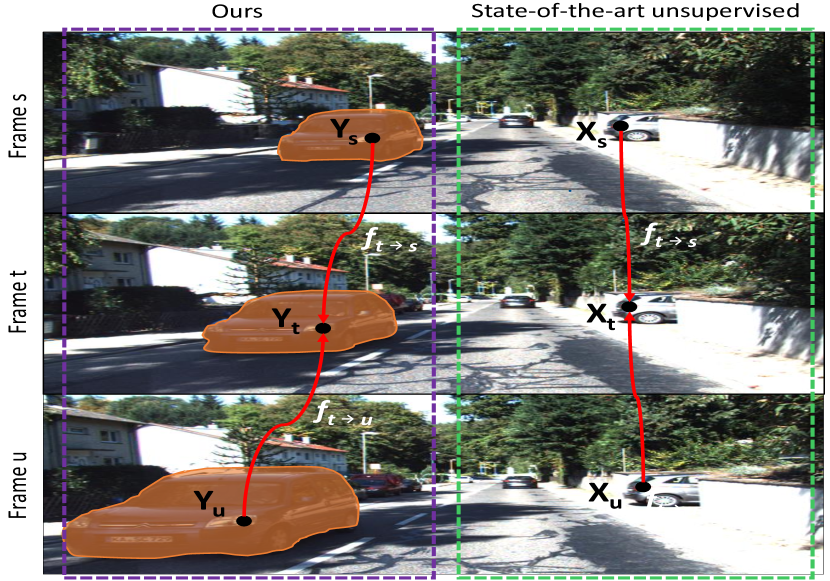
Refer to caption — Figure 1: On the right, state-of-the-art unsupervised learning approach relies on pixel-wise information only, while SIGNet on the left utilizes the semantic information to encode the spatial constraints hence further enhances the geometry prediction.

In Fig 1, we highlight the innovation of our system (on the left) comparing to the existing unsupervised frameworks (on the right) for geometry perception. Traditional unsupervised models learn from the pixel-level feedback (i.e. photo-metric reconstruction loss), whereas SIGNet relies on the key observation that inherent spatial constraints exist in the visual perception problem as shown in Fig 1. Specifically, we exploit the fact that pixels belonging to the same object have additional constraints for the depth and flow prediction.

How can those spatial constraints of the pixels be encoded? We leverage the semantic information as seen in Fig 1 for unsupervised frameworks. Intuitively, semantic information can be interpreted as defining boundaries around a group of pixels whose geometry is closely related. The knowledge of semantic information between different segments of a scene could allow us to easily learn which pixels are correlated, while the object edges could imply sharp depth transition. Furthermore, note that this learning paradigm is practical ²²2Semantic labels can be easily curated on demand on unlabeled data. On the contrary, geometrically informative labels such as flow and depth require additional sensors and careful annotation at the data collection stage. as annotations for semantic prediction tasks such as semantic segmentation are relatively cheaper and easier to acquire. To the best of our knowledge, our work is the first to utilize semantic information in the context of unsupervised learning for geometry perception.

A natural question is how do we combine semantic information with an unsupervised geometric prediction? Our approach to combine the semantic information with RGB input is two-fold: First, we propose a novel way to augment RGB images with semantic information. Second, we propose new loss functions, architecture, and training method. The two-fold approach precisely accounts for spatial constraints in making geometric predictions:

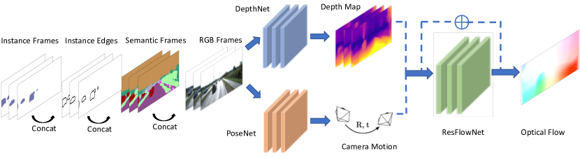
Feature Augmentation: We concatenate the RGB input data with both per-pixel class predictions and instance-level predictions. We use per pixel class predictions to define semantic mask which serves as a guidance signal that eases unsupervised geometric predictions. Moreover, we use the instance-level prediction and split them into two inputs, instance edges and object masks. Instance edges and object masks enable the network to learn the object edges and sharp depth transitions.

Loss Function Augmentation: Second, we augment the loss function to include various semantic losses, which reduces the reliance on semantic features in the evaluation phase. This is crucial when the environment contains less common contextual elements (like in dessert navigation or mining exploitation). We design and experiment with various semantic losses, such as semantic warp loss, masked reconstruction loss, and semantic-aware edge smoothness loss. However, manually designing a loss term which can improve the performance over the feature augmentation technique turns out to be very difficult. The challenge comes from the lack of understanding of error distributions because we are generally biased towards simple, interpretable loss functions that can be sub-optimal in unsupervised learning. Hence, we propose an alternative approach of incorporating a transfer network that learns how to predict semantic mask via a semantic reconstruction loss and provides feedback to improve the depth and pose estimations, which shows considerable improvements in depth and flow prediction.

We empirically evaluate the feature and loss function augmentations on KITTI dataset [14] and compare them with the state-of-the-art unsupervised learning framework [51]. In our experiments we use class-level predictions from DeepLabv3+ [4] trained on Cityscapes [6] and Mask R-CNN [18] trained on MSCOCO [27]. Our key findings:

•

By using semantic segmentation for both feature and loss augmentation, our proposed algorithms improves squared relative error in depth estimation by $28$ % compared to the strong baseline set by state-of-the-art unsupervised GeoNet [51].
•

Feature augmentation alone, combining semantic with instance-level information, leads to larger gains. With both class-level and instance-level features, the squared relative error of the depth predictions improves by $30$ % compared to the baseline.
•

Finally, as for common dynamic object classes (e.g. vehicles) SIGNet shows $39$ % improvement (in squared relative error) for depth predictions and $29$ % improvement in the flow prediction, thereby showing that semantic information is very useful for improving the performance in the dynamic categories of objects. Furthermore, SIGNet is robust to noise in image intensity compared to the baseline.

2 Related Work

Deep Models for Understanding Geometry: Deep models have been widely used in supervised depth estimation [8, 29, 36, 53, 5, 49, 50, 11, 46], tracking, and pose estimation [43, 47, 2, 17] , as well as optical flow predictions [7, 20, 25, 40]. These models have demonstrated superior accuracy and typically faster speed in modern hardware platforms (especially in the case of optical flow estimation) compared to traditional methods. However, achieving good performance with supervised learning requires a large amount of geometry-related labels. The current work addresses this challenge by adopting an unsupervised learning framework for depth, pose, and optical flow estimations.

Deep Models for Semantic Predictions: Deep models are widely applied in semantic prediction tasks, such as image classification [24], semantic segmentation [4], and instance segmentation [18]. In this work, we utilize the effectiveness of the semantic predictions provided by DeepLab v3+ [4] and Mask R-CNN [18] in encoding spatial constraints to accurately predict geometric attributes such as depth and flow. While we particularly choose [4] and [18] for our SIGNet, similar gains can be obtained by using other state-of-the-art semantic prediction methods.

Unsupervised Deep Models for Understanding Geometry: Several recent methods propose to use unsupervised learning for geometry understanding. In particular, Garg et al. [13] uses a warping method based on Taylor expansion. In the context of unsupervised flow prediction, Yu et al. [21] and Ren et al. [37] introduce image reconstruction loss with spatial smoothness constraints. Similar methods are used in Zhou et al. [54] for learning depth and camera ego-motions by ignoring object motions. This is partially addressed by Vijayanarasimhan et al. [41], despite the fact, we note, that the modeling of motion is difficult without introducing semantic information. This framework is further improved with better modeling of the geometry. Geometric consistency loss is introduced to handle occluded regions, in binocular depth learning [16], flow prediction [32] and joint depth, ego-motion and optical flow learning [51]. Mahjourian et al. [31] focuses on improved geometric constraints, Godard et al. [15] proposes several architectural and loss innovations, while Zhan et al. [52] uses reconstruction in the feature space rather than the image space. In contrast, the current work explores using semantic information to resolve ambiguities that are difficult for pure geometric modeling. Methods proposed in the current work are complementary to these recent methods, but we choose to validate our approach on a state-of-the-art framework known as GeoNet [51].

Multi-Task Learning for Semantic and Depth: Multi-task learning [3] achieves better generalization by allowing the system to learn features that are robust across different tasks. Recent methods focus on designing efficient architectures that can predict related tasks using shared features while avoiding negative transfers [35, 19, 30, 34, 23, 12]. In this context, several prior works report promising results combining scene geometry with semantics. For instance, similar to our method Liu et al. [28] uses semantic predictions to provide depth. However, this work is fully supervised and only uses sub-optimal traditional methods. Wang et al. [44], Cross-Stitching [35], UberNet [23] and NDDR-CNN [12] all report improved performance over single-task baselines. But they have not addressed outdoor scenes and unsupervised geometry understanding. Our work is also related to PAD-Net [48]. PAD-Net reports improvements by combining intermediate tasks as inputs to final depth and segmentation tasks. Our method of using semantic input similarly introduces an intermediate prediction task as input to the depth and pose predictions, but we tackle the problem setting where depth labels are not provided.

3 State-of-the-art Unsupervised Geometry Prediction

Prior to presenting our technical approach, we provide a brief overview of state-of-the-art unsupervised depth and motion estimation framework, which is based on image reconstruction from geometric predictions [54, 51]. It trains the geometric prediction models through the reconstructions of a target image from source images. The target and source images are neighboring frames in a video sequence. Note that such a reconstruction is possible only when certain elements of the 3D geometry of the scene are understood: (1) The relative 3D location (and thus the distance) between the camera and each pixel. (2) The camera ego-motion. (3) The motion of pixels. Thus this framework can be used to train a depth estimator and an ego-motion estimator, as well as a optical flow predictor.

Technically, each training sample $\mathcal{I}=\{I_{i}\}_{i=1}^{n}$ consists of $n$ contiguous video frames $I_{i}\in\mathbb{R}^{H\times W\times 3}$ where the center frame $I_{t}$ is the “target frame” and the other frames serve as the “source frame”. In training, a differentiable warping function $f_{t\to s}$ is constructed from the geometry predictions. The warping function is used to reconstruct the target frame $\tilde{I}_{s}\in\mathbb{R}^{H\times W\times 3}$ from source frame $I_{s}$ via bilinear sampling. The level of success in this reconstruction provides training signals through backpropagation to the various ConvNets in the system. A standard loss function to measure reconstruction success is as follows:

\mathcal{L}_{rw}=\alpha\frac{1-\text{SSIM}(I_{t},\tilde{I}_{s})}{2}+(1-\alpha)||I_{t}-\tilde{I}_{s}||_{1}

(1)

where SSIM denotes the structural similarity index [45] and $\alpha$ is set to $0.85$ in [51].

To filter out erroneous predictions while preserving sharp details, the standard practice is to include an edge-aware depth smoothness loss $\mathcal{L}_{ds}$ weighted by image gradients

\mathcal{L}_{ds}=\sum\limits_{p_{t}}|\nabla D(p_{t})|\cdot(e^{-|\nabla I(p_{t})|})^{T}

(2)

where $|\cdot|$ denotes element-wise absolute operation, $\nabla$ is the vector differential operator, and $T$ denotes transpose of gradients. These losses are usually computed from a pyramid of multi-scale predictions. The sum is used as the training target.

While the reconstruction of RGB images is an effective surrogate task for unsupervised learning, it is limited by the lack of semantic information as supervision signals. For example, the system cannot learn the difference between the car and the road if they have similar colors or two neighboring cars with similar colors. When object motion is considered in the models, the learning can mistakenly assign motion to non-moving objects as the geometric constraints are ill-posed. We augment and improve this system by leveraging semantic information.

4 Methods

In this section, we present solutions to enhance geometry predictions with semantic information. Semantic labels can provide rich information on 3D scene geometry. Important details such as 3D location of pixels and their movements can be inferred from a dense representation of the scene semantics. The proposed methods are applicable to a wide variety of recently proposed unsupervised geometry learning frameworks based on photometric reconstruction [54, 16, 51] represented by our baseline framework introduced in Section 3. Our complemented pipeline in test time is illustrated in Fig 2.

4.1 Semantic Input Augmentation

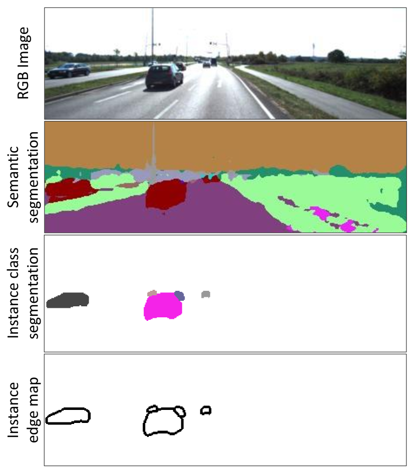
Semantic predictions can improve geometry prediction models when serving as input features. Unlike RGB images, semantic predictions mark objects and contiguous structures with consistent blobs, which provide important information for the learning problem. However, it is uncertain that using semantic labels as input could indeed improve depth and flow predictions since training labels are not available. Semantic information could be lost or distorted, which would end up being a noisy training signal. An important finding of our work is that using semantic predictions as inputs significantly improves the accuracy in geometry predictions, despite the presence of noisy training signal. Input representation and the type of semantic labels have a large impact on the performance of the system. We further illustrate this by Fig 3, where we show various semantic labels (semantic segmentation, instance segmentation, and instance edge) that we use to augment the input. This imposes additional constraints such as depth of the pixels belonging to a particular object (e.g. a vehicle) which helps the learning process. Furthermore, sudden changes in the depth predictions can be inferred from the boundary of vehicles. The semantic labels of the pixels can provide important information to associate pixels across frames.

Encoding Pixel-wise Class Labels: We explored two input encoding techniques for class labels: dense encoding and one-hot encoding. In dense encoding, dense class labels are concatenated along the input channel dimension. The added semantic features are centralized to the range of $[-1,1]$ to be consistent with RGB inputs. In the case of one-hot encoding, the class-level semantic predictions are first expanded to one-hot encoding and then concatenated along the input channel dimension. The labels are represented as one-hot sparse vectors. In this variant, semantic features are not normalized since they have similar value range as the RGB inputs,

Encoding Instance-level Semantic Information: Both dense and one-hot encoding are natural to class-level semantic prediction, where each pixel is only assigned a class label rather than an instance label. Our conjecture is that instance-level semantic information is particular well-suited to improve unsupervised geometric predictions, as it provides accurate information on the boundary between individual objects of the same type. Unlike class-level label, the instance label itself does not have a well-defined meaning. Across different frames, the same label could refer to different object instances. To efficiently represent the instance-level information, we compute the gradient map of a dense instance map and use it as an additional feature channel concatenating to the class label input (dense/one-hot encoding).

Direct Input versus Residual Correction: Complementary to the choice of encoding, we also experiment with different architectures to feed semantic information to the geometry prediction model. In particular, we make a residual prediction using a separate branch that takes in only semantic inputs. Notably, using residual depth prediction leads to further improvement on top of the gains from the direct input methods.

4.2 Semantic Guided Loss Functions

The information from semantic predictions could be diminished due to noisy semantic labels and very deep architectures. Hence, we design training loss functions that are guided by semantic information. In such design, the semantic predictions provide additional loss constraints to the network. In this subsection, we introduce a set of semantic guided loss functions to improve depth and flow predictions.

Semantic Warp Loss: Semantic predictions can help learn scenarios where reconstruction of the RGB image is correct in terms of pixel values but violates obvious semantic correspondences, e.g. matching pixels to incorrect semantic classes and/or instances. In light of this, we propose to reconstruct the semantic predictions in addition of doing so for RGB images. We call this “semantic warping loss” as it is based on warping of the semantic predictions from source frames to the target frame. Let $S_{s}$ be the source frame semantic prediction and $\tilde{S}_{s}^{rig}$ be the warped semantic image, we define semantic warp loss as:

\mathcal{L}_{sem}=||\tilde{S}_{s}^{rig}-S_{t}||_{2}

(3)

The warped loss is added to the baseline framework using a hyper-tuned value of the weight $w$ .

Masking of Reconstruction Loss via Semantics: As described in Section 3, the ambiguity in object motion can lead to sub-optimal learning. Semantic labels can partially resolve this by separating each class of region. Motivated by this observation, we mask the foreground region out to form a set of new images $J_{t,c}^{k}=I_{t,c}\odot S_{t,k}$ for $c=0,1,2$ and $k=0,...,K-1$ where $c$ represents the RGB-channel index, $\odot$ is the element-wise multiplication operator and $S_{s,k}$ is the $k$ -th channel of the binary semantic segmentation ( $K$ classes in total). Similarly we can obtain $\tilde{J}_{s,c}^{rig,k}=\tilde{I}_{s,c}^{rig}\odot S_{t,k}$ for $c=0,1,2$ and $k=0,...,K-1$ . Finally, the image similarity loss is defined as:

\mathcal{L}_{rw}^{\prime}=\sum\limits_{k=0}^{K-1}\alpha\frac{1-\text{SSIM}(J_{t}^{k},\tilde{J}_{s}^{rig,k})}{2}+(1-\alpha)||J_{t}^{k}-\tilde{J}_{s}^{rig,k}||_{1}

(4)

Semantic-Aware Edge Smoothness Loss: Equation 2 uses RGB to infer edge locations when enforcing smooth regions of depth. This could be improved by including an edge map computed from semantic predictions. Given a semantic segmentation result $S_{t}$ , we define a weight matrix $M_{t}\in[0,1]^{H\times W}$ where the weight is low (close to zero) on class boundary regions and high (close to one) on other regions. We propose a new image similarity loss as:

	$\displaystyle\mathcal{L}_{rw}^{\prime\prime}$	$\displaystyle=\sum\limits_{k=0}^{K-1}\alpha\frac{1-\text{SSIM}(I_{t}\odot M_{t},\tilde{I}_{s}^{rig}\odot M_{t})}{2}$		(5)
		$\displaystyle+(1-\alpha)\|\|I_{t}\odot M_{t}-\tilde{I}_{s}^{rig}\odot M_{t}\|\|_{1}$		(5)

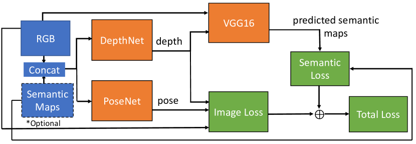
Semantic Loss by Transfer Network: Motivated by the observation that high-quality depth maps usually depict object classes and background region, we designed a novel transfer network architecture. As shown in Fig 4 the transfer network block receives predicted depth maps along with the original RGB images and outputs semantic labels. The transfer network introduces a semantic reconstruction loss term to the objective function to force the predicted depth maps to be richer in contextual sense, hence refines the depth estimation. For implementation, we choose the ResNet-50 as the backbone and alter the dimensions for the input and output convolutional layers to be consistent with the segmentation task. The network generates one-hot encoded heatmaps and use cross-entropy as the semantic similarity measure.

5 Experiments

To quantify the benefits that semantic information brings to geometry-based learning, we designed experiments similar to [51]. First, we showed our model’s depth prediction performance on KITTI dataset [14], which outperformed state-of-the-art unsupervised and supervised models. Then we designed ablation studies to analyze each individual component’s contribution. Finally, we presented improvements in flow predictions and revisited the performance gains using a category-specific evaluation.

5.1 Implementation Details

To make a fair comparison with state-of-the-art models [8, 54, 51], we divided KITTI 2015 dataset into train set (40238 images) and test set (697 images) according to the rules from Eigen et al [8]. We used DeepLabv3+ [4] (pretrained on [6]) for semantic segmentation and Mask-RCNN [18] (pretrained on [27]) for instance segmentation. Similar to the hyper-parameter settings in [51], we used Adam optimizer [22] with initial learning rate as 2e-4, set batch size to 4 per GPU and trained our modified DepthNet and PoseNet modules for 250000 iterations with random shuffling and data augmentation (random scaling, cropping and RGB perturbation). The training took 10 hours on two GTX1080Ti.

5.2 Monocular Depth Evaluation on KITTI

We augmented the image sequences with corresponding semantic and instance segmentation sequences and adopted the scale normalization suggested in [42]. In the evaluation stage, the ground truth depth maps were generated by projecting 3D Velodyne LiDAR points to the image plane. Followed by [51], we clipped our depth predictions within 0.001m to 80m and calibrated the scale by the medium number of the ground truth. The evaluation results are shown in Table 1, where all the metrics are introduced in [8]. Our model benefits significantly from feature augmentation and surpasses the state-of-the-art methods substantially in both supervised and unsupervised fields.

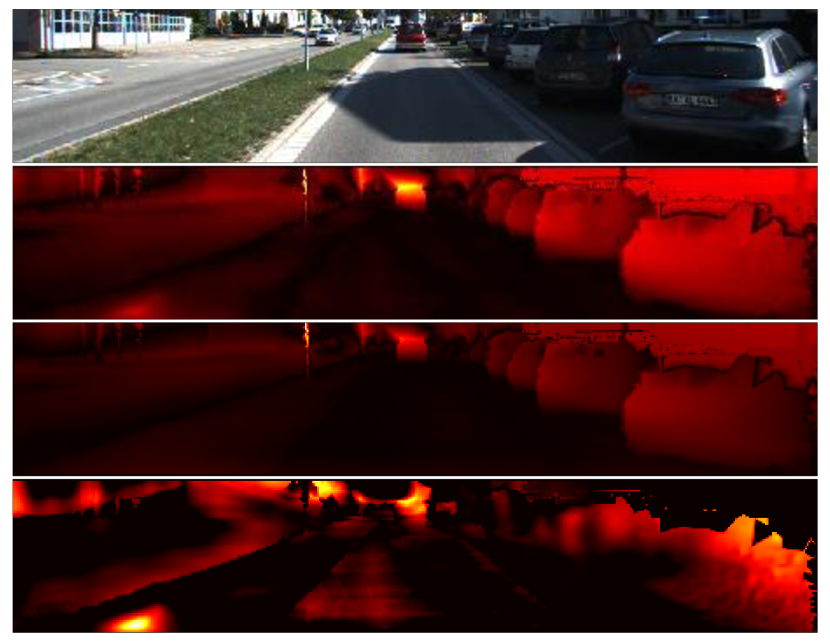
Moreover, we found a correlation between the improvement region and object classes. We visualized the absolute relative error (AbsRel) among image plane from our model and from the baseline. As shown in Fig 5, most of the improvements come from regions containing objects. This indicates that the network is able to learn the concept of objects to improve the depth prediction by rendering extra semantic information.

Method	Supervised	Error-related metrics				Accuracy-related metrics
Method	Supervised	Abs Rel	Sq Rel	RSME	RSME log	$\delta<1.25$	$\delta<1.25^{2}$	$\delta<1.25^{3}$
Eigen et al. [8] Coarse	Depth	0.214	1.605	6.653	0.292	0.673	0.884	0.957
Eigen et al. [8] Fine	Depth	0.203	1.548	6.307	0.282	0.702	0.890	0.957
Liu et al. [29]	Depth	0.202	1.614	6.523	0.275	0.678	0.895	0.965
Godard et al. [16]	Pose	0.148	1.344	5.927	0.247	0.803	0.922	0.964
Zhou et al. [54] updated	No	0.183	1.595	6.709	0.270	0.734	0.902	0.959
Yin et al. [51]	No	0.155	1.296	5.857	0.233	0.793	0.931	0.973
Ours	No	0.133	0.905	5.181	0.208	0.825	0.947	0.981
(improved by)	No	14.04%	30.19%	11.55%	10.85%	3.14%	1.53%	0.80%

Table 1: Monocular depth results on KITTI 2015 [33] by the split of Eigen et al. [8] (Our model used scale normalization.)

5.3 Ablation Studies

Here we took a deeper look of our model, testified its robustness under noise from observations, and presented variations of our framework to show promising explorations for future researchers. In the following experiments, we kept all the other parameters the same in [51] and applied the same training/evaluation strategies mentioned in Section 5.2

How much gain from various feature augmentation?
We tried out different combinations and forms of semantic/instance-level inputs based on “Yin et al” [51] with scale normalization. From Table 2, our first conclusion is that any meaningful form of extra input can ameliorate the model, which is straightforward. Secondly, when we use “Semantic” and “Instance class” for feature augmentation, one-hot encoding tends to outperform the dense map form. Conceivably one-hot encoding stores richer information in its structural formation, whereas dense map only contains discrete labels which may be more difficult for learning. Moreover, using both “Semantic” and “Instance class” can provide further gain, possibly due to the different label distributions of the two datasets. Labels from Cityscape [6] cover both background and foreground concepts, while the COCO dataset [27] focuses more on objects. At last, when we combined one-hot encoded “Semantic” and “Instance class” along with “Instance id” edge features, the network exploited the most from scene understanding, hence greatly enhanced the performance.

Semantic	Instance	Instance	Error-related metrics				Accuracy-related metrics
Semantic	class	id	Abs Rel	Sq Rel	RSME	RSME log	$\delta<1.25$	$\delta<1.25^{2}$	$\delta<1.25^{3}$
			0.149	1.060	5.567	0.226	0.796	0.935	0.975
Dense			0.142	0.991	5.309	0.216	0.814	0.943	0.980
One-hot			0.139	0.949	5.227	0.214	0.818	0.945	0.980
	Dense		0.142	0.986	5.325	0.218	0.812	0.943	0.978
	One-hot		0.141	0.976	5.272	0.215	0.811	0.942	0.979
		Edge	0.145	1.037	5.314	0.217	0.807	0.943	0.978
	Dense	Edge	0.142	0.969	5.447	0.219	0.808	0.941	0.978
One-hot	One-hot	Edge	0.133	0.905	5.181	0.208	0.825	0.947	0.981

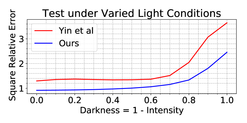
Table 2: Depth prediction performance gains due to different semantic sources and forms. (Scale normalization was used.)

Can our model survive under low lighting conditions?
To testify our model’s robustness for varied lighting conditions, we multiplied a scalar between 0 and 1 to RGB inputs in the evaluation. Fig 6 showed that our model still holds equal performance to [51] when the intensity drops to $30$ %.

Which module needs extra information the most?
We fed semantics to only DepthNet or PoseNet to see the difference in their performance gain. From Table 3 we can see that compared to DepthNet, PoseNet learns little from the semantics to help depth prediction. Therefore we tried to feed the semantics to a new PoseNet with the same structure as the original one and compute the predicted poses by taking the sum from two different PoseNets, which led to performance gain; however, performance gain was not observed from applying the same method to DepthNet.

DepthNet	PoseNet	Error-related metrics				Accuracy-related metrics
DepthNet	PoseNet	Abs Rel	Sq Rel	RSME	RSME log	$\delta<1.25$	$\delta<1.25^{2}$	$\delta<1.25^{3}$
		0.149	1.060	5.567	0.226	0.796	0.935	0.975
Channel		0.145	0.957	5.291	0.216	0.805	0.943	0.980
	Channel	0.147	1.076	5.385	0.223	0.808	0.938	0.975
Channel	Channel	0.139	0.949	5.227	0.214	0.818	0.945	0.980
Extra Net	Channel	0.147	1.036	5.593	0.226	0.803	0.937	0.975
Channel	Extra Net	0.135	0.932	5.241	0.211	0.821	0.945	0.980

Table 3: Each module’s contribution toward performance gain from semantics. (Scale normalization was used.)

How to be “semantic-free” in evaluation?
Though semantic helps depth prediction, this idea relies on semantic features during the evaluation phase. If semantic is only utilized in the loss, it would not be needed in evaluation. We attempted to introduce a handcrafted semantic loss term as a weight guidance among image plane but it didn’t work well. Also we designed a transfer network which uses the predicted depth to predict semantic maps along with a reconstruction error to help in the training stage. The result in Table 4 shows a better result can be obtained by training from pretrained models.

Checkpoint	Transfer	Error-related metrics				Accuracy-related metrics
Checkpoint	Network	Abs Rel	Sq Rel	RSME	RSME log	$\delta<1.25$	$\delta<1.25^{2}$	$\delta<1.25^{3}$
Yin et al. [51]		0.155	1.296	5.857	0.233	0.793	0.931	0.973
Yin et al. [51]	Yes	0.150	1.141	5.709	0.231	0.792	0.934	0.974
Yin et al. [51] +sn		0.149	1.060	5.567	0.226	0.796	0.935	0.975
Yin et al. [51] +sn	Yes	0.145	0.994	5.422	0.222	0.806	0.939	0.976

Table 4: Gains in depth prediction using our proposed Transfer Network. (+sn: “using scale normalization”.)

5.4 Optical Flow Estimation on KITTI

Using our best model for DepthNet and PoseNet in Section 5.2, we conducted rigid flow and full flow evaluation on KITTI [14]. We generated the rigid flow from estimated depth and pose, and compared with [51]. Our model performed better in all the metrics shown in Table 5.

Method	End Point Error		Accuracy
Method	Noc	All	Noc	All
Yin et al. [51]	23.5683	29.2295	0.2345	0.2237
Ours	22.3819	26.8465	0.2519	0.2376

Table 5: Rigid flow prediction from first stage on KITTI on non-occluded regions(Noc) and overall regions(All).

Method	End Point Error
Method	Noc	All
DirFlowNetS	6.77	12.21
Yin et al. [51]	8.05	10.81
Ours	7.66	13.91

Table 6: Full flow prediction on KITTI 2015 on non-occluded regions(Noc) and overall regions(All). Results from DirFlowNetS are shown in [51]

We further appended the semantic warping loss introduced in Section 4.2 to ResFlowNet in [51] and trained our model on KITTI stereo for 1600000 iterations. As demonstrated in Table 6, flow prediction got improved in non-occluded region compared to [51] and our model produced comparable results in overall regions.

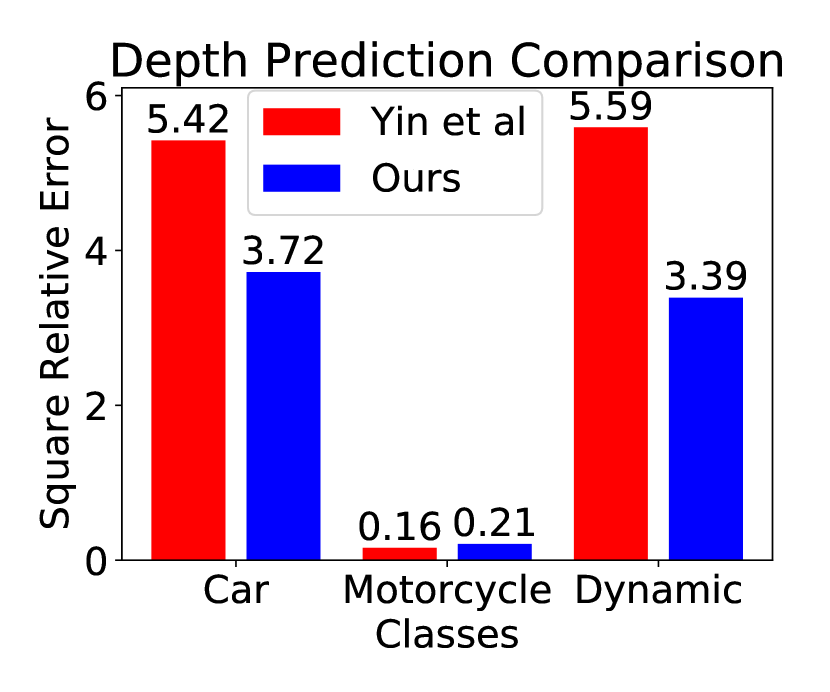
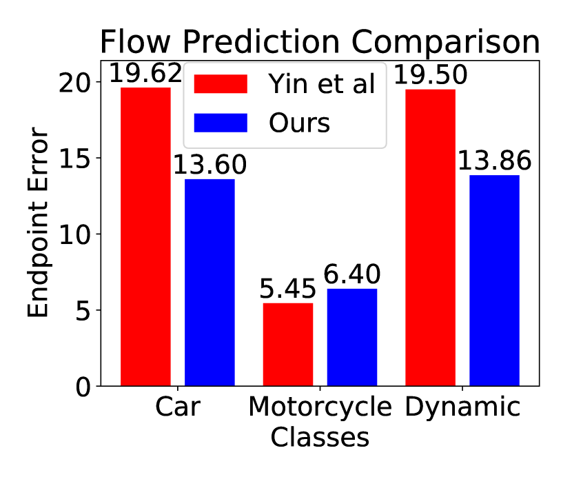
5.5 Category-Specific Metrics Evaluation

This section will present the improvements by semantic categories. As shown in the bar-chart in Fig 7, most improvements were shown in “Vehicle” and “Dynamic” classes³³3For “Dynamic” classes, we choose “person”, “rider”, “car”, “truck”, “bus”, “train”, “motorcycle” and “bicycle” classes as defined in [6], where errors are generally large. Our network did not improve much for other less frequent categories, such as “Motorcycle”, which are generally more difficult to segment in images.

6 Conclusion

In SIGNet, we strive to achieve robust performance for depth and flow perception without using geometric labels. To achieve this goal, SIGNet utilizes semantic and instance segmentation to create spatial constraints on the geometric attributes of the pixels. We present novel methods of feature augmentation and loss augmentation to include semantic labels in the geometry predictions. This work presents a first of a kind approach which moves away from pixel-level to object-level depth and flow predictions. Most notably, our method significantly surpasses the state-of-the-art solution for monocular depth estimation. In the future, we would like to extend our SIGNet to various sensor modalities (IMU, LiDAR or thermal).

Acknowledgement: This work was supported by UCSD faculty startup (Prof. Bharadia), Toyota InfoTechnology Center and Center for Wireless communication at UCSD.

References

[1] Michael Bloesch, Jan Czarnowski, Ronald Clark, Stefan Leutenegger, and Andrew J Davison. Codeslam-learning a compact, optimisable representation for dense visual slam. arXiv preprint arXiv:1804.00874, 2018.
[2] Arunkumar Byravan and Dieter Fox. Se3-nets: Learning rigid body motion using deep neural networks. In Robotics and Automation (ICRA), 2017 IEEE International Conference on, pages 173–180. IEEE, 2017.
[3] Rich Caruana. Multitask learning. Mach. Learn., 28(1):41–75, July 1997.
[4] Liang-Chieh Chen, Yukun Zhu, George Papandreou, Florian Schroff, and Hartwig Adam. Encoder-decoder with atrous separable convolution for semantic image segmentation. arXiv preprint arXiv:1802.02611, 2018.
[5] Weifeng Chen, Zhao Fu, Dawei Yang, and Jia Deng. Single-image depth perception in the wild. In Proceedings of the 30th International Conference on Neural Information Processing Systems, NIPS’16, pages 730–738, USA, 2016. Curran Associates Inc.
[6] Marius Cordts, Mohamed Omran, Sebastian Ramos, Timo Rehfeld, Markus Enzweiler, Rodrigo Benenson, Uwe Franke, Stefan Roth, and Bernt Schiele. The cityscapes dataset for semantic urban scene understanding. In Proceedings of the IEEE conference on computer vision and pattern recognition, pages 3213–3223, 2016.
[7] Alexey Dosovitskiy, Philipp Fischer, Eddy Ilg, Philip Hausser, Caner Hazirbas, Vladimir Golkov, Patrick van der Smagt, Daniel Cremers, and Thomas Brox. Flownet: Learning optical flow with convolutional networks. In The IEEE International Conference on Computer Vision (ICCV), December 2015.
[8] David Eigen, Christian Puhrsch, and Rob Fergus. Depth map prediction from a single image using a multi-scale deep network. In Advances in neural information processing systems, pages 2366–2374, 2014.
[9] Xiaohan Fei, Alex Wang, and Stefano Soatto. Geo-supervised visual depth prediction. arXiv preprint arXiv:1807.11130, 2018.
[10] Philipp Fischer, Alexey Dosovitskiy, Eddy Ilg, Philip Häusser, Caner Hazırbaş, Vladimir Golkov, Patrick Van der Smagt, Daniel Cremers, and Thomas Brox. Flownet: Learning optical flow with convolutional networks. arXiv preprint arXiv:1504.06852, 2015.
[11] Huan Fu, Mingming Gong, Chaohui Wang, Kayhan Batmanghelich, and Dacheng Tao. Deep ordinal regression network for monocular depth estimation. In The IEEE Conference on Computer Vision and Pattern Recognition (CVPR), June 2018.
[12] Yuan Gao, Qi She, Jiayi Ma, Mingbo Zhao, Wei Liu, and Alan L. Yuille. Nddr-cnn: Layer-wise feature fusing in multi-task cnn by neural discriminative dimensionality reduction. CoRR, abs/1801.08297, 2018.
[13] Ravi Garg, G VijayKumarB., and Ian D. Reid. Unsupervised cnn for single view depth estimation: Geometry to the rescue. In ECCV, 2016.
[14] Andreas Geiger, Philip Lenz, and Raquel Urtasun. Are we ready for autonomous driving? the kitti vision benchmark suite. In Computer Vision and Pattern Recognition (CVPR), 2012 IEEE Conference on, pages 3354–3361. IEEE, 2012.
[15] Clément Godard, Oisin Mac Aodha, and Gabriel J. Brostow. Digging into self-supervised monocular depth estimation. CoRR, abs/1806.01260, 2018.
[16] Clément Godard, Oisin Mac Aodha, and Gabriel J Brostow. Unsupervised monocular depth estimation with left-right consistency. In CVPR, volume 2, page 7, 2017.
[17] Daniel Gordon, Ali Farhadi, and Dieter Fox. Re ³: Real-time recurrent regression networks for visual tracking of generic objects. IEEE Robotics and Automation Letters, 3(2):788–795, 2018.
[18] Kaiming He, Georgia Gkioxari, Piotr Dollár, and Ross Girshick. Mask r-cnn. In Computer Vision (ICCV), 2017 IEEE International Conference on, pages 2980–2988. IEEE, 2017.
[19] Keke He, Zhanxiong Wang, Yanwei Fu, Rui Feng, Yu-Gang Jiang, and Xiangyang Xue. Adaptively weighted multi-task deep network for person attribute classification. In Proceedings of the 25th ACM International Conference on Multimedia, MM ’17, pages 1636–1644, New York, NY, USA, 2017. ACM.
[20] Eddy Ilg, Nikolaus Mayer, Tonmoy Saikia, Margret Keuper, Alexey Dosovitskiy, and Thomas Brox. Flownet 2.0: Evolution of optical flow estimation with deep networks. In The IEEE Conference on Computer Vision and Pattern Recognition (CVPR), July 2017.
[21] J Yu Jason, Adam W Harley, and Konstantinos G Derpanis. Back to basics: Unsupervised learning of optical flow via brightness constancy and motion smoothness. In European Conference on Computer Vision, pages 3–10. Springer, 2016.
[22] Diederik P Kingma and Jimmy Ba. Adam: A method for stochastic optimization. arXiv preprint arXiv:1412.6980, 2014.
[23] I. Kokkinos. Ubernet: Training a universal convolutional neural network for low-, mid-, and high-level vision using diverse datasets and limited memory. In 2017 IEEE Conference on Computer Vision and Pattern Recognition (CVPR), pages 5454–5463, July 2017.
[24] Alex Krizhevsky, Ilya Sutskever, and Geoffrey E. Hinton. Imagenet classification with deep convolutional neural networks. Commun. ACM, 60(6):84–90, May 2017.
[25] Wei-Sheng Lai, Jia-Bin Huang, and Ming-Hsuan Yang. Semi-supervised learning for optical flow with generative adversarial networks. In NIPS, 2017.
[26] Konstantinos-Nektarios Lianos, Johannes L Schönberger, Marc Pollefeys, and Torsten Sattler. Vso: Visual semantic odometry. In Proceedings of the European Conference on Computer Vision (ECCV), pages 234–250, 2018.
[27] Tsung-Yi Lin, Michael Maire, Serge Belongie, James Hays, Pietro Perona, Deva Ramanan, Piotr Dollár, and C Lawrence Zitnick. Microsoft coco: Common objects in context. In European conference on computer vision, pages 740–755. Springer, 2014.
[28] Beyang Liu, Stephen Gould, and Daphne Koller. Single image depth estimation from predicted semantic labels. 2010 IEEE Computer Society Conference on Computer Vision and Pattern Recognition, pages 1253–1260, 2010.
[29] Fayao Liu, Chunhua Shen, Guosheng Lin, and Ian D Reid. Learning depth from single monocular images using deep convolutional neural fields. IEEE Trans. Pattern Anal. Mach. Intell., 38(10):2024–2039, 2016.
[30] Yongxi Lu, Abhishek Kumar, Shuangfei Zhai, Yu Cheng, Tara Javidi, and Rogerio Feris. Fully-adaptive feature sharing in multi-task networks with applications in person attribute classification. In The IEEE Conference on Computer Vision and Pattern Recognition (CVPR), July 2017.
[31] Reza Mahjourian, Martin Wicke, and Anelia Angelova. Unsupervised learning of depth and ego-motion from monocular video using 3d geometric constraints. In The IEEE Conference on Computer Vision and Pattern Recognition (CVPR), June 2018.
[32] Simon Meister, Junhwa Hur, and Stefan Roth. UnFlow: Unsupervised learning of optical flow with a bidirectional census loss. In AAAI, New Orleans, Louisiana, Feb. 2018.
[33] Moritz Menze and Andreas Geiger. Object scene flow for autonomous vehicles. In Proceedings of the IEEE Conference on Computer Vision and Pattern Recognition, pages 3061–3070, 2015.
[34] Elliot Meyerson and Risto Miikkulainen. Beyond shared hierarchies: Deep multitask learning through soft layer ordering. CoRR, abs/1711.00108, 2017.
[35] Ishan Misra, Abhinav Shrivastava, Abhinav Gupta, and Martial Hebert. Cross-stitch networks for multi-task learning. 2016 IEEE Conference on Computer Vision and Pattern Recognition (CVPR), pages 3994–4003, 2016.
[36] N.Mayer, E.Ilg, P.Häusser, P.Fischer, D.Cremers, A.Dosovitskiy, and T.Brox. A large dataset to train convolutional networks for disparity, optical flow, and scene flow estimation. In IEEE International Conference on Computer Vision and Pattern Recognition (CVPR), 2016. arXiv:1512.02134.
[37] Zhe Ren, Junchi Yan, Bingbing Ni, Bin Liu, Xiaokang Yang, and Hongyuan Zha. Unsupervised deep learning for optical flow estimation. In AAAI, volume 3, page 7, 2017.
[38] Ashutosh Saxena, Sung H Chung, and Andrew Y Ng. Learning depth from single monocular images. In Advances in neural information processing systems, pages 1161–1168, 2006.
[39] Ashutosh Saxena, Min Sun, and Andrew Y Ng. Make3d: Learning 3d scene structure from a single still image. IEEE transactions on pattern analysis and machine intelligence, 31(5):824–840, 2009.
[40] Deqing Sun, Xiaodong Yang, Ming-Yu Liu, and Jan Kautz. Pwc-net: Cnns for optical flow using pyramid, warping, and cost volume. In The IEEE Conference on Computer Vision and Pattern Recognition (CVPR), June 2018.
[41] Sudheendra Vijayanarasimhan, Susanna Ricco, Cordelia Schmid, Rahul Sukthankar, and Katerina Fragkiadaki. Sfm-net: Learning of structure and motion from video. arXiv preprint arXiv:1704.07804, 2017.
[42] Chaoyang Wang, José Miguel Buenaposada, Rui Zhu, and Simon Lucey. Learning depth from monocular videos using direct methods. In Proceedings of the IEEE Conference on Computer Vision and Pattern Recognition, pages 2022–2030, 2018.
[43] Lijun Wang, Wanli Ouyang, Xiaogang Wang, and Huchuan Lu. Visual tracking with fully convolutional networks. In Proceedings of the IEEE international conference on computer vision, pages 3119–3127, 2015.
[44] Peng Wang, Xiaohui Shen, Zhe Lin, Scott Cohen, Brian Price, and Alan L. Yuille. Towards unified depth and semantic prediction from a single image. In The IEEE Conference on Computer Vision and Pattern Recognition (CVPR), June 2015.
[45] Zhou Wang, Alan C Bovik, Hamid R Sheikh, and Eero P Simoncelli. Image quality assessment: from error visibility to structural similarity. IEEE transactions on image processing, 13(4):600–612, 2004.
[46] Ke Xian, Chunhua Shen, Zhiguo Cao, Hao Lu, Yang Xiao, Ruibo Li, and Zhenbo Luo. Monocular relative depth perception with web stereo data supervision. In The IEEE Conference on Computer Vision and Pattern Recognition (CVPR), June 2018.
[47] Yu Xiang, Tanner Schmidt, Venkatraman Narayanan, and Dieter Fox. Posecnn: A convolutional neural network for 6d object pose estimation in cluttered scenes. arXiv preprint arXiv:1711.00199, 2017.
[48] Dan Xu, Wanli Ouyang, Xiaogang Wang, and Nicu Sebe. Pad-net: Multi-tasks guided prediction-and-distillation network for simultaneous depth estimation and scene parsing. CoRR, abs/1805.04409, 2018.
[49] Dan Xu, Elisa Ricci, Wanli Ouyang, Xiaogang Wang, and Nicu Sebe. Multi-scale continuous crfs as sequential deep networks for monocular depth estimation. In The IEEE Conference on Computer Vision and Pattern Recognition (CVPR), July 2017.
[50] Dan Xu, Wei Wang, Hao Tang, Hong Liu, Nicu Sebe, and Elisa Ricci. Structured attention guided convolutional neural fields for monocular depth estimation. In The IEEE Conference on Computer Vision and Pattern Recognition (CVPR), June 2018.
[51] Zhichao Yin and Jianping Shi. Geonet: Unsupervised learning of dense depth, optical flow and camera pose. In Proceedings of the IEEE Conference on Computer Vision and Pattern Recognition (CVPR), volume 2, 2018.
[52] Huangying Zhan, Ravi Garg, Chamara Saroj Weerasekera, Kejie Li, Harsh Agarwal, and Ian Reid. Unsupervised learning of monocular depth estimation and visual odometry with deep feature reconstruction. In The IEEE Conference on Computer Vision and Pattern Recognition (CVPR), June 2018.
[53] Ziyu Zhang, Alexander G. Schwing, Sanja Fidler, and Raquel Urtasun. Monocular object instance segmentation and depth ordering with cnns. 2015 IEEE International Conference on Computer Vision (ICCV), pages 2614–2622, 2015.
[54] Tinghui Zhou, Matthew Brown, Noah Snavely, and David G Lowe. Unsupervised learning of depth and ego-motion from video. In CVPR, volume 2, page 7, 2017.

Supplementary Material for SIGNet

Additional ablation studies on loss augmentations: As mentioned in our paper, the heuristic loss functions are not effective even after careful hyper-parameter tuning. This motivated us to design a learnable loss function (transfer network), which does improve upon the baseline as shown in Table 4 of our paper.

Method	Error metrics				Accuracy $(\delta<)$
Method	AbsRel	SqRel	RSME	RSME_log	$1.25^{1}$	$1.25^{2}$	$1.25^{3}$
Yin et al.[51]	0.155	1.296	5.857	0.233	0.793	0.931	0.973
Warp Loss	0.169	1.246	6.233	0.254	0.750	0.917	0.968
Mask Loss	0.165	1.204	5.593	0.232	0.769	0.926	0.974
Edge Loss	0.163	1.230	5.961	0.243	0.774	0.924	0.970
Transfer	0.150	1.141	5.709	0.231	0.792	0.934	0.974

Table 1: Depth predictions for different loss augmentations (without using scale normalization). Here Warp Loss, Mask Loss and Edge Loss are on par or not as good as the baseline, whereas Transfer Network surpasses the baseline in almost all the metrics.

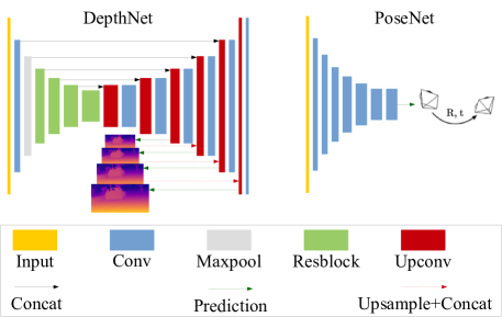
Why does ”ExtraNet” only work for PoseNet? In the ablation studies in Section 5.3, we tested the contribution of semantic information in each module. The result suggests that vanilla PoseNet benefits from semantics only marginally, which might due to its simple structure. By adding Extra Network (”ExtraNet”) to PoseNet, our model gained further improvement. ”ExtraNet” does not benefit DepthNet because the latter has already had a complicated structure as shown in Figure 1.

More visualization results for depth estimation: In the rest of the supplementary material, we will present extra visualization results to help readers understand where our semantic-aided model improved the most. We compared the prediction result from our best model in Table 1 with Yin et al. [51] and ground truth. We followed [13] to plot the prediction result using disparity heatmaps. The following results show that our model can gain improvement from regions belonging to cars and other dynamic classes.