A new reduction strategy for special negative sectors of planar two-loop integrals without Laporta algorithm

Adam Kardos

University of Debrecen, Faculty of Science and Technology, Institute of Physics

H-4010 Debrecen, PO Box 105, Hungary

Abstract

In planar two-loop integrals there is a dedicated sector such that when its index is zero, the two-loop integral decomposes into the product of two one-loop integrals. We show an alternative reduction strategy for these sectors when their index is negative using the Baikov representation. This reduction strategy is free from the Laporta algorithm. It follows a top-down approach and is much faster than approaches based on the brute-force, conventional integration by parts identities.

December 2018

The extremely successful operation of LHC resulted in high-quality data taken by all its experiments. This data is being used to produce high-accuracy measurements for several processes to stress-test the standard model. From the theory side equally high-precision predictions are required to be able to draw definite conclusions from these comparisons. After the full automation of NLO calculations in QCD [1, 2, 3]. Tools are becoming available to perform NNLO calculations [4, 5, 6, 7, 8, 9, 10] and automation at NNLO is put on the horizon. One crucial ingredient of these calculations is the two-loop amplitude.

In the two-loop amplitude the occurring tensor integrals have to be expressed on an integral basis. One way to do so is by means of integration by part (IBP) identities [11, 12] by which these tensor integrals are written as a linear combination of master integrals times coefficients depending on kinematic invariants and space-time dimension. In practice Laporta’s algorithm [13] is used to derive IBP identities for reduction. This algorithm is implemented in several computer programs to tackle the problem of reduction [14, 15, 16, 17, 18]. As for the computation of remaining master integrals the last decade witnessed an unprecedented advancement. This spans from how to write these master integrals as differential equations [19, 20, 21] through the definition of new functions [22, 23, 24, 25, 26] to new techniques and tools to attack the resulting equations [27, 28].

These techniques are put to the ultimate test when two-loop five-parton amplitudes were calculated [29, 30, 31, 32, 33]. In a realistic calculation due to the numerator structure propagators not only appear with positive but also with negative and large exponents. As it was found in Ref. [31] the real bottle-neck for reduction came from those integrals where propagators had a large negative exponent.

At the two-loop level planar integrals are special in the sense that they only contain one propagator depending on both loop momenta and in the absence of this propagator the two-loop integral can be written as the product of two one-loop tensor integrals. Because of this the sector associated to this propagator is treated as a special one. If this nature of the special sector is not recognized and the reduction is carried out as an ordinary one the reduction time can be unnecessarily large.

In this work we present an alternative reduction strategy for this special sector of two-loop planar integrals. In the heart of this reduction strategy stands the Baikov representation [34, 35, 36, 37, 38, 39, 40]. In general it was found that a reduction strategy using the Baikov representation results in very cumbersome systems of equations [21]. However, for this special sector the Baikov representation offers a nice way to perform the reduction by disentangling the two-loop integral into two one-loop integrals. The resulting one-loop tensor integrals are much easier to run an IBP-based or Passarino-Veltman reduction on them. The special sector having a negative index the original two-loop integral can also be considered as the product of two one-loop tensor integrals on which a Passarino-Veltman reduction can in principle be done. Nonetheless with our reduction strategy we can offer one more option laying between the blind IBP and traditional Passarino-Veltman reduction.

In order to derive our reduction strategy for the special sector we first introduce the Baikov representation for a general $L$-loop Feynman integral. In this effort we closely follow the notation of Ref. [41]. An $L$-loop Feynman-integral with $E$ independent external legs the integral can be written as

$$I^{(L)}_{\alpha_{1}\dots\alpha_{N}} =\int\left(\prod_{i=1}^{L}\frac{\mathrm{d}^{d}\ell_{i}}{i\pi^{d/2}}\right)\frac{1}{D_{1}^{\alpha_{1}}\cdots D_{N}^{\alpha_{N}}}\,,$$ (1)

where $N=\frac{L(L+1)}{2}+LE$, $\alpha_{i}$ are the positive or negative integer indices and $D_{i}$ are the propagator factors. Every propagator factor can be written in the form of

$$D_{a} =\sum_{i,j=1}^{L}A_{a}^{ij}(\ell_{i}\cdot\ell_{j})+\sum_{i=1}^{L}\sum_{j=1}^{E}A_{a}^{i(j+L)}(\ell_{i}\cdot p_{j})+f_{a}\,,\quad a\in{1,\dots,N}$$ (2)

where $A_{a}^{ij}$ are the coefficient matrices and $f_{a}$ comprise the dot products involving only external momenta and internal masses. The definition of coefficient matrices and the $f_{a}$ functions allow us to write the multiloop Feynman integral in the form of Baikov:

$$I^{(L)}_{\alpha_{1}\dots\alpha_{N}} =\mathcal{N}\int\frac{\mathrm{d}x_{1}\cdots\mathrm{d}x_{N}}{x_{1}^{\alpha_{1}}\cdots x_{N}^{\alpha_{N}}}\left(\mathcal{P}_{N}^{L}(x_{1}-f_{1},\dots,x_{N}-f_{N})\right)^{\frac{d-L-E-1}{2}}$$ (3)

with

$$\mathcal{P}_{N}^{L}(x_{1},\dots,x_{N}) =\left.G(\ell_{1},\dots,\ell_{L},p_{1},\dots,p_{E})\right|_{s_{ij}=\sum_{a=1}^{N}A_{a}^{ij}x_{a}}\,,$$ (4)

where $G$ is the Gram determinant composed of momenta appearing in its argument, the $x$’s are called the Baikov variables and $\mathcal{N}$ is a factor depending on the topology, dimension and external momenta – not relevant to the forthcoming discussion – the exact definition can be found, e.g., in Ref. [41].

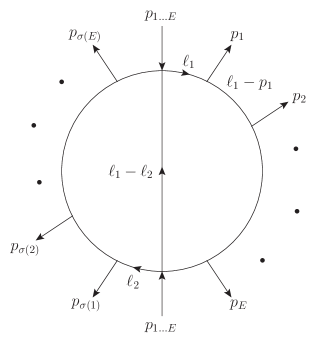
Figure 1: A general two-loop planar topology with $E+1$ external legs and $\sigma\in S_{E}$.

Due to construction the Baikov polynomial is at most quadratic in each Baikov variable. In a generic planar two-loop Feynman integral it is always possible to have only one propagator containing both loop momenta. Such a Feynman integral is depicted on Fig. 1. The Baikov polynomial is the determinant of the Gram matrix where we substitute linear combinations of $x$’s for the dot products. If using $q_{i}\in\{\ell_{1},\dots,\ell_{L},p_{1},\dots,p_{E}\},\,i\in\{1,\dots,L+E\}$ the Gram determinant can be written as:

$$G(\ell_{1},\dots,\ell_{L},p_{1},\dots,p_{E}) =\sum_{\sigma\in S_{L+E}}\left(\mathrm{sgn}(\sigma)\prod_{i=1}^{L+E}q_{i}\cdot q_{\sigma_{i}}\right)\,,$$ (5)

which is just the definition of the determinant for a $(L+E)\times(L+E)$ matrix where each matrix element is a genuine dot product and $S_{L+E}$ is the set containing all permutations of the $L+E$ elements. It is apparent from Eq. (5) that when $L=2$ the terms proportional to $(\ell_{1}\cdot\ell_{2})^{2}$ beside of this factor can only contain dot products of external momenta. Thus for a two-loop planar topology if $x_{a}$ assigned to the propagator containing both loop momenta in the corresponding Baikov polynomial the terms having $x_{a}^{2}$ dependence beside this factor can only contain external invariants or internal masses. Because of the quadratic dependence on Baikov variables, the Baikov polynomial can be written as

$$\mathcal{P}^{L}_{N}(x_{1},\dots,x_{N})=f(x_{1},\dots,x_{a-1},x_{a+1},\dots,x_{N})(x_{a}^{+}-x_{a})(x_{a}-x_{a}^{-})\,,$$ (6)

the integration region for $x_{a}$ extends from $x_{a}^{-}$ to $x_{a}^{+}$ and with the obvious, gracious property of $\left.\mathcal{P}_{N}^{L}(x_{1},\dots,x_{N})\right|_{x_{a}=x_{a}^{-}}=\left.\mathcal{P}_{N}^{L}(x_{1},\dots,x_{N})\right|_{x_{a}=x_{a}^{+}}=0$. To simplify our notation we define our multiloop Feynman integral in terms of the Baikov variables such that

$$I^{(L)}_{\alpha_{1}\dots\alpha_{N}} =\mathcal{N}\int\frac{\prod\mathrm{d}x_{i}}{\prod x_{i}^{\alpha_{i}}}\mathcal{P}^{n}\,,$$ (7)

where $\mathcal{N}$ is the factor already used in Eq. (3), $n=\frac{d-L-E-1}{2}$ and for brevity we dropped both sub- and superscript and argument of the Baikov polynomial, $\mathcal{P}$. We are interested in the two-loop planar case where the special sector, the one having both loop momenta, has a negative exponent, can be written as:

$$I^{(2)}_{\alpha_{1}\dots\alpha_{N}} =\mathcal{N}\int\frac{\prod\mathrm{d}x_{i}}{\prod_{{i\neq a}}x_{i}^{\alpha_{i}}}x_{a}^{-\alpha_{a}}\mathcal{P}^{n}\,,\quad\alpha_{a}<0\,.$$ (8)

First, let us examine the case where $\alpha_{a}=-1$. We know that the coefficient of the term proportional to $x_{a}^{2}$ in the Baikov polynomial does not depend on other $x$’s thus the coefficient of the term proportional to $x_{a}$ in $\partial_{x_{a}}\mathcal{P}$ cannot have any dependence on $x$’s either. Hence by substituting $\partial_{x_{a}}\mathcal{P}$ for $x_{a}$:

$$\mathcal{N}\int\frac{\prod\mathrm{d}x_{i}}{\prod_{{i\neq a}}x_{i}^{\alpha_{i}}}(\partial_{a}\mathcal{P})\mathcal{P}^{n} =\mathcal{C}_{\alpha_{1}\dots\alpha_{N}}I^{(2)}_{\alpha_{1}\dots\alpha_{N}}+\sum_{\begin{subarray}{c}\{\beta\}\\ \beta_{a}=0\end{subarray}}\mathcal{C}_{\beta_{1}\dots\beta_{N}}I^{(2)}_{\beta_{1}\dots\beta_{N}}=$$

$$=\mathcal{C}_{\alpha_{1}\dots\alpha_{N}}I^{(2)}_{\alpha_{1}\dots\alpha_{N}}+\sum_{\begin{subarray}{c}\{\beta\}\\ \beta_{a}=0\end{subarray}}\mathcal{C}_{\beta_{1}\dots\beta_{N}}\left(I^{(1)}\otimes I^{(1)}\right)_{\beta_{1}\dots\beta_{N}}\,,$$ (9)

where as a short-hand $\partial_{a}$ was used for $\partial_{x_{a}}$, $\{\beta\}$ stands for a set of indices. The source of these extra index configurations is the polynomial nature of $\partial_{a}\mathcal{P}$ which does not only contain $x_{a}$ with some prefactors but additional terms too. The additional terms can depend on several Baikov variables and hence can alter the power these variables appear on. The $\mathcal{C}$ coefficients only depend on external kinematics and masses. As the special sector appears on the zeroth power in all the terms in the right hand side but the first one and this is the only sector containing both loop momenta these integrals are products of two one-loop Feynman integrals, hence the notation $I^{(1)}\otimes I^{(1)}$. In order to use this observation in the reduction of two-loop planar integrals we have to turn this into an IBP relation. To this end note that the integration limits for all the Baikov variables are determined by the condition $\mathcal{P}=0$. Keeping this in mind we can come up with the following relation:

$$\int\frac{\prod\mathrm{d}x_{i}}{\prod_{{i\neq a}}x_{i}^{\alpha_{i}}}(\partial_{a}\mathcal{P})\mathcal{P}^{n} =\frac{1}{n+1}\int\frac{\prod\mathrm{d}x_{i}}{\prod_{{i\neq a}}x_{i}^{\alpha_{i}}}\partial_{a}\left(\mathcal{P}^{n+1}\right)=$$

$$=\widetilde{\mathcal{C}}_{\alpha_{1}\dots\alpha_{N}}I^{(2)}_{\alpha_{1}\dots\alpha_{N}}+\sum_{\begin{subarray}{c}\{\beta\}\\ \beta_{a}=0\end{subarray}}\widetilde{\mathcal{C}}_{\beta_{1}\dots\beta_{N}}\left(I^{(1)}\otimes I^{(1)}\right)_{\beta_{1}\dots\beta_{N}}=0\,,$$ (10)

where the reader should notice that the integration over $x_{a}$ only results in vanishing surface terms since the only dependence on $x_{a}$ in the integrand is in the Baikov polynomial in the second step. The tilde over the coefficients is introduced because for simplicity we divided Eq. (10) by $\mathcal{N}$, $\widetilde{\mathcal{C}}=\mathcal{C}/\mathcal{N}$.

This way we can always write a two-loop planar Feynman integral having the special inverse propagator on the first power as a sum of products of one-loop integrals. To do so we do not have to perform the full reduction, instead, we can start with the special sector. Upon reduction the original integral becomes a product of two one-loop tensor integrals for which the reductions are much simple.

So far we only addressed the case when the exponent of the special sector is $-1$. To have a useful alternate reduction strategy for this kind of integrals we have to devise a strategy even for the case when $\alpha_{a}<-1$ as well. If the propagator corresponding to the special sector is raised to the power $\alpha_{a}$, due to the properties outlined previously of the Baikov polynomial, the following relation holds:

$$\int\frac{\prod\mathrm{d}x_{i}}{\prod_{{i\neq a}}x_{i}^{\alpha_{i}}}x_{a}^{-\alpha_{a}-1}(\partial_{a}\mathcal{P})\mathcal{P}^{n} =\widetilde{\mathcal{C}}_{\alpha_{1}\dots\alpha_{N}}I^{(2)}_{\alpha_{1}\dots\alpha_{N}}+\sum_{\begin{subarray}{c}\{\beta\}\\ \alpha_{a}<\beta_{a}\end{subarray}}\widetilde{\mathcal{C}}_{\beta_{1}\dots\beta_{N}}I^{(2)}_{\beta_{1}\dots\beta_{N}}\,,$$ (11)

where the first term on the right-hand side is the integral we want to reduce, with some prefactors, and the remaining terms are further two-loop integrals where the special sector appears on a lower power.

This relation can be turned into an IBP identity by recasting it into:

$$\int\frac{\prod\mathrm{d}x_{i}}{\prod_{{i\neq a}}x_{i}^{\alpha_{i}}}x_{a}^{-\alpha_{a}-1}(\partial_{a}\mathcal{P})\mathcal{P}^{n} =\frac{1}{n+1}\int\frac{\prod\mathrm{d}x_{i}}{\prod_{{i\neq a}}x_{i}^{\alpha_{i}}}\partial_{a}\left(x_{a}^{-\alpha_{a}-1}\mathcal{P}^{n+1}\right)+$$

$$+\frac{1+\alpha_{a}}{n+1}\int\frac{\prod\mathrm{d}x_{i}}{\prod_{{i\neq a}}x_{i}^{\alpha_{i}}}x_{a}^{-\alpha_{a}-2}\mathcal{P}^{n+1}\,,$$ (12)

where the first term on the right-hand side is zero because it is a total derivative in $x_{a}$. Thus we find that:

$$0 =\int\frac{\prod\mathrm{d}x_{i}}{\prod_{{i\neq a}}x_{i}^{\alpha_{i}}}x_{a}^{-\alpha_{a}-1}(\partial_{a}\mathcal{P})\mathcal{P}^{n}-\frac{1+\alpha_{a}}{n+1}\int\frac{\prod\mathrm{d}x_{i}}{\prod_{{i\neq a}}x_{i}^{\alpha_{i}}}x_{a}^{-\alpha_{a}-2}\mathcal{P}\,\mathcal{P}^{n}\,,$$ (13)

where both $x_{a}^{-\alpha_{a}-1}\partial_{a}\mathcal{P}$ and $x_{a}^{-\alpha_{a}-2}\mathcal{P}$ have terms proportional to $x_{a}^{-\alpha_{a}}$. Collecting these terms we notice that the rest have the Baikov variable $x_{a}$ on a lower power thus our original integral can be expressed through ones having lower rank in $x_{a}$. Notice also that the special case immediately follows from setting $\alpha_{a}=-1$.

Reductions can be further simplified when the Baikov polynomial is written in the form of:

$$\mathcal{P} =\sum_{j=1}^{N}g_{j}\frac{\partial\mathcal{P}}{\partial x_{j}}+b\,,$$ (14)

where both $g_{j}$ and $b$ are polynomials in the Baikov variables. Thus the IBP relation for the general case can be cast into the form of:

$$0 =\int\frac{\prod\mathrm{d}x_{i}}{\prod_{{i\neq a}}x_{i}^{\alpha_{i}}}x_{a}^{-\alpha_{a}-1}(\partial_{a}\mathcal{P})\mathcal{P}^{n}-\frac{1+\alpha_{a}}{n+1}\left\{\sum_{j=1}^{N}\int\frac{\prod\mathrm{d}x_{i}}{\prod_{{i\neq a}}x_{i}^{\alpha_{i}}}x_{a}^{-\alpha_{a}-2}g_{j}(\partial_{j}\mathcal{P})\mathcal{P}^{n}+\right.$$

$$+\left.\int\frac{\prod\mathrm{d}x_{i}}{\prod_{{i\neq a}}x_{i}^{\alpha_{i}}}x_{a}^{-\alpha_{a}-2}b\,\mathcal{P}^{n}\right\}\,.$$ (15)

This form turns out to be very useful since it can be used to further simplify the reduction of a given integral. For some $j$ the monomial coefficient of $(\partial_{j}\mathcal{P})\mathcal{P}^{n}$ in the integrand can become independent of $x_{j}$ thus the term can be dropped being a total derivative in $x_{j}$.

In practice when given a planar two-loop integral with the mixed propagator on the $\alpha_{a}$ power we calculate the Baikov polynomial for the integral family and the decomposition of Eq. (14). Plugging these into Eq. (15) with $\alpha_{a}$ and $n=\frac{d-L-E-1}{2}$ we can identify the integral we started with and it can be expressed with integrals having the special sector on a lower power. This procedure can be continued until we have only one integral having the special sector on the minus first power and all the other integrals are just products of one-loop tensor integrals. Solving for this integral and substituting back we performed the reduction of our original two-loop tensor integral in terms of products of one-loop tensor integrals. So the reduction of the integral follows a simple top-down strategy, free from the Laporta algorithm.

In this letter we showed an alternate reduction strategy for a sector of planar two-loop tensor integrals which contains both loop momenta and the corresponding inverse propagator appears in the numerator with some positive power. The basis of the reduction is the Baikov representation of the integral and the exploitation of basic properties of this representation. As the reduction is carried out, the original two-loop tensor integral becomes a sum of products of two one-loop tensor integrals. We tested our reduction strategy with Laporta-based reduction programs available in the literature and we found agreement for all, including the most complicated topologies, like the pentabox and massive doublebox. We found that with a non-optimized Mathematica implementation of our strategy it was possible to carry out the reduction even for tensor integrals with high rank in the mixed sector on a single laptop. On the other hand using commercially available software we had to use a rack-mounted computer with 48 cores equipped with significant amount of memory to perform the same operation. In an NNLO calculation we encounter both two-loop amplitudes and interference terms of two one-loop amplitudes. The reduction of the former to master integrals is a tedious procedure but with our method applied to the special sector of the planar part a significant amount of time can be saved. In case of the latter the appearance of the special sector is natural. The presence of these contributions makes it cumbersome to use numerical routines to evaluate the tensor integrals. By applying our prescription to the problem the mixed inverse propagator disappears and the contribution becomes the product of two genuine one-loop tensor integrals attackable even with numerical programs dedicated to one-loop amplitude reductions.

The author is grateful to Costas Papadopoulos for so many fruitful discussions on the topic and for his comments on the manuscript, Zoltán Trócsányi for carefully reading the manuscript and Manfred Kraus for providing far-from trivial two-loop planar tensor integrals to test the scheme. We acknowledge financial support from the Premium Postdoctoral Fellowship program of the Hungarian Academy of Sciences. This work was supported by grant K 125105 of the National Research, Development and Innovation Fund in Hungary.

References

- [1] T. Gleisberg, S. Hoeche, F. Krauss, M. Schonherr, S. Schumann, F. Siegert, and J. Winter, Event generation with SHERPA 1.1, JHEP 02 (2009) 007, [arXiv:0811.4622].
- [2] G. Bevilacqua, M. Czakon, M. V. Garzelli, A. van Hameren, A. Kardos, C. G. Papadopoulos, R. Pittau, and M. Worek, HELAC-NLO, Comput. Phys. Commun. 184 (2013) 986–997, [arXiv:1110.1499].
- [3] J. Alwall, R. Frederix, S. Frixione, V. Hirschi, F. Maltoni, O. Mattelaer, H. S. Shao, T. Stelzer, P. Torrielli, and M. Zaro, The automated computation of tree-level and next-to-leading order differential cross sections, and their matching to parton shower simulations, JHEP 07 (2014) 079, [arXiv:1405.0301].
- [4] S. Catani and M. Grazzini, HNNLO: A Monte Carlo program to compute Higgs boson production at hadron colliders, PoS RADCOR2007 (2007) 046, [arXiv:0802.1410].
- [5] S. Catani, L. Cieri, G. Ferrera, D. de Florian, and M. Grazzini, Vector boson production at hadron colliders: a fully exclusive QCD calculation at NNLO, Phys. Rev. Lett. 103 (2009) 082001, [arXiv:0903.2120].
- [6] R. Gavin, Y. Li, F. Petriello, and S. Quackenbush, W Physics at the LHC with FEWZ 2.1, Comput. Phys. Commun. 184 (2013) 208–214, [arXiv:1201.5896].
- [7] A. Gehrmann-De Ridder, T. Gehrmann, E. W. N. Glover, and G. Heinrich, EERAD3: Event shapes and jet rates in electron-positron annihilation at order , Comput. Phys. Commun. 185 (2014) 3331, [arXiv:1402.4140].
- [8] R. Boughezal, J. M. Campbell, R. K. Ellis, C. Focke, W. Giele, X. Liu, F. Petriello, and C. Williams, Color singlet production at NNLO in MCFM, Eur. Phys. J. C77 (2017), no. 1 7, [arXiv:1605.0801].
- [9] M. Grazzini, S. Kallweit, and M. Wiesemann, Fully differential NNLO computations with MATRIX, Eur. Phys. J. C78 (2018), no. 7 537, [arXiv:1711.0663].
- [10] J. Currie, A. Gehrmann-De Ridder, T. Gehrmann, N. Glover, A. Huss, and J. Pires, Jet cross sections at the LHC with NNLOJET, in 14th DESY Workshop on Elementary Particle Physics: Loops and Legs in Quantum Field Theory 2018 (LL2018) St Goar, Germany, April 29-May 4, 2018, 2018. arXiv:1807.0605.
- [11] F. V. Tkachov, A Theorem on Analytical Calculability of Four Loop Renormalization Group Functions, Phys. Lett. 100B (1981) 65–68.
- [12] K. G. Chetyrkin and F. V. Tkachov, Integration by Parts: The Algorithm to Calculate beta Functions in 4 Loops, Nucl. Phys. B192 (1981) 159–204.
- [13] S. Laporta, High precision calculation of multiloop Feynman integrals by difference equations, Int. J. Mod. Phys. A15 (2000) 5087–5159, [hep-ph/0102033].
- [14] C. Anastasiou and A. Lazopoulos, Automatic integral reduction for higher order perturbative calculations, JHEP 07 (2004) 046, [hep-ph/0404258].
- [15] A. von Manteuffel and C. Studerus, Reduze 2 - Distributed Feynman Integral Reduction, arXiv:1201.4330.
- [16] R. N. Lee, Presenting LiteRed: a tool for the Loop InTEgrals REDuction, arXiv:1212.2685.
- [17] A. V. Smirnov, FIRE5: a C++ implementation of Feynman Integral REduction, Comput. Phys. Commun. 189 (2015) 182–191, [arXiv:1408.2372].
- [18] P. Maierhöfer, J. Usovitsch, and P. Uwer, Kira—A Feynman integral reduction program, Comput. Phys. Commun. 230 (2018) 99–112, [arXiv:1705.0561].
- [19] J. M. Henn, Multiloop integrals in dimensional regularization made simple, Phys. Rev. Lett. 110 (2013) 251601, [arXiv:1304.1806].
- [20] C. G. Papadopoulos, Simplified differential equations approach for Master Integrals, JHEP 07 (2014) 088, [arXiv:1401.6057].
- [21] J. Bosma, K. J. Larsen, and Y. Zhang, Differential equations for loop integrals in Baikov representation, Phys. Rev. D97 (2018), no. 10 105014, [arXiv:1712.0376].
- [22] A. B. Goncharov, Multiple polylogarithms, cyclotomy and modular complexes, Math. Res. Lett. 5 (1998) 497–516, [arXiv:1105.2076].
- [23] A. B. Goncharov, Multiple polylogarithms and mixed Tate motives, math/0103059.
- [24] A. B. Goncharov, M. Spradlin, C. Vergu, and A. Volovich, Classical Polylogarithms for Amplitudes and Wilson Loops, Phys. Rev. Lett. 105 (2010) 151605, [arXiv:1006.5703].
- [25] J. Ablinger, J. Blümlein, and C. Schneider, Analytic and Algorithmic Aspects of Generalized Harmonic Sums and Polylogarithms, J. Math. Phys. 54 (2013) 082301, [arXiv:1302.0378].
- [26] J. Broedel, C. Duhr, F. Dulat, B. Penante, and L. Tancredi, Elliptic symbol calculus: from elliptic polylogarithms to iterated integrals of Eisenstein series, arXiv:1803.1025.
- [27] R. N. Lee, Reducing differential equations for multiloop master integrals, JHEP 04 (2015) 108, [arXiv:1411.0911].
- [28] O. Gituliar and V. Magerya, Fuchsia: a tool for reducing differential equations for Feynman master integrals to epsilon form, Comput. Phys. Commun. 219 (2017) 329–338, [arXiv:1701.0426].
- [29] S. Badger, G. Mogull, A. Ochirov, and D. O’Connell, A Complete Two-Loop, Five-Gluon Helicity Amplitude in Yang-Mills Theory, JHEP 10 (2015) 064, [arXiv:1507.0879].
- [30] T. Gehrmann, J. M. Henn, and N. A. Lo Presti, Analytic form of the two-loop planar five-gluon all-plus-helicity amplitude in QCD, Phys. Rev. Lett. 116 (2016), no. 6 062001, [arXiv:1511.0540]. [Erratum: Phys. Rev. Lett.116,no.18,189903(2016)].
- [31] H. A. Chawdhry, M. A. Lim, and A. Mitov, Two-loop five-point massless QCD amplitudes within the IBP approach, arXiv:1805.0918.
- [32] S. Badger, C. Bronnum-Hansen, H. B. Hartanto, and T. Peraro, Analytic helicity amplitudes for two-loop five-gluon scattering: the single-minus case, arXiv:1811.1169.
- [33] S. Abreu, J. Dormans, F. Febres Cordero, H. Ita, and B. Page, Analytic Form of the Planar Two-Loop Five-Gluon Scattering Amplitudes in QCD, arXiv:1812.0458.
- [34] P. A. Baikov, Explicit solutions of the multiloop integral recurrence relations and its application, Nucl. Instrum. Meth. A389 (1997) 347–349, [hep-ph/9611449].
- [35] P. A. Baikov, Explicit solutions of the three loop vacuum integral recurrence relations, Phys. Lett. B385 (1996) 404–410, [hep-ph/9603267].
- [36] V. A. Smirnov and M. Steinhauser, Solving recurrence relations for multiloop Feynman integrals, Nucl. Phys. B672 (2003) 199–221, [hep-ph/0307088].
- [37] R. N. Lee, Calculating multiloop integrals using dimensional recurrence relation and -analyticity, Nucl. Phys. Proc. Suppl. 205-206 (2010) 135–140, [arXiv:1007.2256].
- [38] A. G. Grozin, Integration by parts: An Introduction, Int. J. Mod. Phys. A26 (2011) 2807–2854, [arXiv:1104.3993].
- [39] R. N. Lee and A. A. Pomeransky, Critical points and number of master integrals, JHEP 11 (2013) 165, [arXiv:1308.6676].
- [40] M. Harley, F. Moriello, and R. M. Schabinger, Baikov-Lee Representations Of Cut Feynman Integrals, JHEP 06 (2017) 049, [arXiv:1705.0347].
- [41] H. Frellesvig and C. G. Papadopoulos, Cuts of Feynman Integrals in Baikov representation, JHEP 04 (2017) 083, [arXiv:1701.0735].