An Accurate Analytic Model for the Thermal Sunyaev-Zel’dovich One-Point PDF

Abstract

Non-Gaussian statistics of late-time cosmological fields contain information beyond that captured in the power spectrum. Here we focus on one such example: the one-point probability distribution function (PDF) of the thermal Sunyaev-Zel’dovich (tSZ) signal in maps of the cosmic microwave background (CMB). It has been argued that the one-point PDF is a near-optimal statistic for cosmological constraints from the tSZ signal, as most of the constraining power in tSZ $N$-point functions is contained in their amplitudes (rather than their shapes), which probe differently-weighted integrals over the halo mass function. In this paper, we develop a new analytic halo model for the tSZ PDF, discarding simplifying assumptions made in earlier versions of this approach. In particular, we account for effects due to overlaps of the tSZ profiles of different halos, as well as effects due to the clustering of halos. We verify the accuracy of our analytic model via comparison to numerical simulations. We demonstrate that this more accurate model is necessary for the analysis of the tSZ PDF in upcoming CMB experiments. The novel formalism developed here may be useful in modeling the one-point PDF of other cosmological observables, such as the weak lensing convergence field.

I Introduction

Cosmological inference has traditionally focused on measurements of the power spectrum (or its real-space analogue, the two-point correlation function). For a Gaussian random field, this approach is sensible, as the power spectrum contains all statistical information in the data. The primary cosmic microwave background (CMB) temperature and polarization anisotropies are canonical examples of such Gaussian fields Planck2018params ; Planck2015NG ; WMAP9params . However, although the initial conditions for cosmic structure formation captured in the CMB are consistent with Gaussianity, non-Gaussian features inevitably develop in the late-time universe, due to non-linear gravitational evolution and complex baryonic physics on small scales. Thus, the information content of late-time cosmological data sets, e.g., weak gravitational lensing maps or maps of the galaxy distribution, is not completely captured by the power spectrum. For highly non-Gaussian fields, the amount of additional information in higher-order statistics can be significant.

In Ref. Hill2014ACTPDF (hereafter H14), it was argued that the one-point probability distribution function (PDF) is a near-optimal non-Gaussian statistic for cosmological inference from maps of the thermal Sunyaev-Zel’dovich (tSZ) effect. The tSZ effect is the up-scattering of CMB photons to higher energies due to Thomson scattering off hot, free electrons, which produces a unique distortion in the energy spectrum of the CMB ZS1969 ; SZ1970 . The tSZ effect probes the integrated pressure of free electrons along the line-of-sight (LOS); thus it is a biased tracer of free electrons, due to its dependence on the product of the electron number density and temperature. In particular, because of this temperature dependence, the tSZ signal is predominantly sourced by electrons in galaxy groups and clusters, where electrons are virialized to high temperatures. As the distribution of such objects in our Hubble volume is nearly Poissonian, maps of the tSZ effect are extremely non-Gaussian, dominated by individual rare, bright sources. H14 proposed the tSZ one-point PDF as an efficient statistic with which to extract the information in this non-Gaussianity.

Non-Gaussian properties of the tSZ signal have long been used for cosmological constraints, in the more familiar guise of inferring parameters via measurements of the halo mass function, in which candidate clusters are identified via the tSZ effect, their existence is confirmed and redshifts are estimated via multi-wavelength follow-up observations, and their masses are estimated via follow-up observations and/or scaling relations (e.g., Hasselfield2013 ; Planck2015clusters ; Bocquet2018 ). However, this approach utilizes only the brightest tSZ objects in the sky, e.g., those with signal-to-noise ($S/N$) greater than some threshold in the map. An alternative strategy has thus been developed in the past two decades, in which “indirect” statistics of the tSZ signal are directly utilized as cosmological probes, such as the power spectrum (e.g., Komatsu-Seljak2002 ; Hill-Pajer2013 ; McCarthy2014 ; Horowitz-Seljak2017 ; Sievers2013 ; George2015 ; Planck2013ymap ; Planck2015ymap ), bispectrum/skewness Wilson2012 ; Bhattacharya2013 ; Crawford2014 ), and cross-power spectra with gravitational lensing maps (e.g., HS2014 ; vanWaerbeke2014 ; Hojjatti2017 ). In such applications, no individual galaxy clusters are identified; instead, these statistics utilize information in objects below the $S/N$ threshold for individual detection, modeling their properties at the ensemble level. In particular, it has been shown that tSZ statistics beyond the power spectrum contain a significant amount of cosmological information beyond that contained in cluster counts (for current $S/N$ thresholds) or the power spectrum Wilson2012 ; Bhattacharya2013 ; Hill-Sherwin2013 ; Hill2014ACTPDF .

A unifying feature of these statistical tSZ analyses is that their cosmological constraining power arises almost entirely from the one-halo term. In other words, these statistics are just indirect methods of counting halos, weighted in different ways. For example, the tSZ power spectrum is dominated by the one-halo term at all $\ell\gtrsim 50$ Komatsu-Kitayama1999 ; Komatsu-Seljak2002 ; Hill-Pajer2013 . Thus, rather than deriving cosmological constraints from spatial clustering information, these statistics do so via the halo mass function. In particular, due to the tSZ signal’s bias toward electrons in high-mass (i.e., high-temperature) halos, these statistics probe the exponential tail of the mass function, which makes them very sensitive probes of the amplitude of fluctuations, $\sigma_{8}$ (e.g., Komatsu-Seljak2002 ; Wilson2012 ; Hill-Sherwin2013 ; Bhattacharya2013 ). Importantly, this sensitivity to $\sigma_{8}$ is almost entirely encoded in the amplitude of these statistics, rather than their shape; due to the one-halo term’s dominance (as mentioned above), the shape encodes information about intracluster medium (ICM) physics (and weak dependence on non-$\sigma_{8}$ cosmological parameters), while the amplitude is directly connected to integrals over the halo mass function, and hence $\sigma_{8}$. This underlies the argument presented in H14 that the one-point PDF is an optimal statistic for cosmological inference from the tSZ signal. The one-point PDF effectively captures the information in the amplitude of all $N$-point functions (or zero-lag moments), at the expense of information contained in the shape of the $N$-point functions (we anticipate that some shape information could be restored by considering the PDF on multiple smoothing scales, but such issues are not the focus of this paper). While not optimal for constraining ICM parameters, the tSZ PDF does allow for the breaking of degeneracies between these parameters and $\sigma_{8}$, due to the different dependence of each moment on these parameters and $\sigma_{8}$ (this is a generalization of the argument for parameter degeneracy-breaking using the tSZ two- and three-point functions presented in Ref. Hill-Sherwin2013 ).

The improved cosmological constraining power of the tSZ PDF over other tSZ statistics was demonstrated in practice in H14, which analyzed data from the Atacama Cosmology Telescope (ACT) at 148 GHz (using some 218 GHz data for foreground control as well). Compared to an analysis of the same data using the tSZ skewness Wilson2012 , the error bar on $\sigma_{8}$ was decreased by a factor of two in H14 (yielding $\sigma_{8}=0.793\pm 0.018$), simply due to the improved cosmological sensitivity of the tSZ PDF over the skewness alone. However, the $S/N$ of the measurement was not high enough to simultaneously constrain cosmological and ICM parameters (though the latter were marginalized over in obtaining the final $\sigma_{8}$ constraint). The Planck Collaboration subsequently applied the PDF statistic to an analysis of their component-separated tSZ map, obtaining $\sigma_{8}=0.77\pm 0.02$ Planck2015ymap .

However, the theoretical modeling that was developed for the tSZ PDF in H14 made several simplifying assumptions, limiting its utility in upcoming measurements (its sufficiency for the analysis of the ACT data in H14 was verified explicitly using end-to-end simulations). The analytic halo model of H14 assumed that clusters were Poisson-distributed on the sky and did not overlap, allowing the tSZ PDF to be computed via a simple integral over the mass function, given a model for the tSZ profile of each halo. The primary goal of this paper is to remove these simplifying assumptions and generalize the analytic model from H14, thereby allowing its use in analyses of the tSZ PDF from ongoing and upcoming CMB experiments (e.g., Advanced ACT Henderson2016 , SPT-3G Benson2014 , Simons Observatory SO2018 , and CMB-S4 CMBS4ScienceBook ). The assumptions are related to the distribution of halos sourcing the tSZ signal. In H14, it was assumed that these halos were sufficiently rare that they never overlapped on the sky. For massive clusters, this assumption is valid, but as the tSZ signal of progressively lower mass halos is included in the PDF, this assumption breaks down. For an experiment with relatively high noise levels (e.g., $\gtrsim 20\,\mu{\rm K}$-arcmin with $\sim$arcmin-scale beams), the assumption is valid, since low-mass clusters are subsumed into the noise. However, current and upcoming CMB experiments have noise levels well below this threshold, necessitating an improved model.

The other assumption from H14 that we will discard in this analysis is the neglect of halo clustering effects. These effects are relevant due to the LOS projection inherent in the tSZ signal. Note that the one-point PDF of 3D cosmic fields (i.e., the “voxel” PDF) does not receive any clustering contributions: as long as halo exclusion is enforced, only the one-halo term is necessary to compute the 3D PDF in the formalism used in this paper. For projected 2D fields, however, this is not true. Due to halo clustering, there is an excess probability for two halos to overlap along the LOS, compared to the Poisson expectation. For the tSZ field, we will find (Fig. 1 below) that the clustering effect is relatively weak, but for future extensions of this formalism to the weak lensing convergence field, we expect that it will be significant.

The remainder of this paper is organized as follows. In §II, we review the halo model formalism of H14 and the associated assumptions, before proceeding to generalize the model in §III and compare the results to those obtained in the simpler approach. In §IV, we compare results from our analytic halo model to those obtained from numerical simulations, demonstrating its validity and accuracy. In §V, we use the analytic model to investigate the physical origin of the tSZ PDF signal. §VI presents the cosmological and ICM parameter dependence of the tSZ PDF. We then include noise and non-tSZ foregrounds in §VII, and demonstrate the sufficiency of our new model for the analysis of upcoming, high-precision CMB data sets. We conclude in §VIII.

Our fiducial cosmology is flat $\Lambda$CDM with dimensionless Hubble constant $h=0.7$, matter density $\Omega_{\rm M}=0.25$, spectral index $n_{s}=0.96$, $\sigma_{8}=0.8$, baryon density $\Omega_{\rm B}=0.043$, sum of the neutrino masses $\Sigma m_{\nu}=0$ eV, and CMB temperature $T_{\rm CMB}=2.726\,{\rm K}$.

II Background and Previous Model

H14 introduced a novel, simple analytic model for the tSZ one-point PDF. Here we review this model and its assumptions, laying the groundwork for the more accurate model derived in the following section.

The tSZ signal is quantified by the Compton-$y$ parameter, which measures the integrated pressure of free electrons along the LOS:

$$y(\mathbf{n})=\frac{\sigma_{\rm T}}{m_{e}c^{2}}\int_{\rm LOS}dr\,n_{e}(r,\mathbf{n})k_{\rm B}T_{e}(r,\mathbf{n})\,,$$ (1)

where $\sigma_{\rm T}$ is the Thomson cross-section, $m_{e}c^{2}$ is the electron rest-mass energy, $r$ is physical distance along the LOS, $n_{e}$ is the electron number density, $k_{\rm B}$ is Boltzmann’s constant, and $T_{e}$ is the electron temperature.

The tSZ effect produces a non-blackbody distortion in the energy spectrum of the CMB, which is negative (positive) at frequencies below (above) $\approx 218$ GHz. Defining the dimensionless frequency $x\equiv h_{\rm Pl}\nu/(k_{\rm B}T_{\rm CMB})$, where $h_{\rm Pl}$ is Planck’s constant and $\nu$ is the photon frequency, the tSZ spectral function is given by:

$$g(\nu)=x\coth(x/2)-4\,.$$ (2)

The tSZ-induced fluctuations in the CMB temperature field are then given by:

$$\frac{\Delta T_{\rm tSZ}(\mathbf{n},\nu)}{T_{\rm CMB}}=g(\nu)y(\mathbf{n})\,.$$ (3)

In this work, we neglect relativistic corrections to the tSZ effect (e.g., Nozawa2006 ), which are important for massive, hot clusters; these effects must be included in an actual data analysis (as they were in H14). Throughout the rest of the paper, our results will generally be given either in terms of Compton-$y$ or in terms of the tSZ field at a reference frequency of 148 GHz, where $g(148\,{\rm GHz})=-0.97881$. We will also typically denote the tSZ-induced temperature fluctuation as simply $T\equiv\Delta T_{\rm tSZ}$.

We denote the (differential) tSZ one-point PDF as $P(y)$. The binned version of the PDF used in much of this work is given by

$$p_{i}=\int_{y_{i}}^{y_{i+1}}dy\,P(y)\,.$$ (4)

The concept underpinning the H14 model is to note that $p_{i}$ quantifies the fraction of sky subtended by Compton-$y$ values in the range $[y_{i},y_{i+1}]$. Thus, for a single spherically symmetric halo with an azimuthally symmetric projected $y$-profile $y(\theta)$, this would correspond to the area in the annulus between $\theta(y_{i})$ and $\theta(y_{i+1})$, where $\theta(y_{i})$ is the angular distance from the center of the halo to the radius where $y(\theta)=y_{i}$. If one then makes the approximation that halos sourcing the tSZ signal are sufficiently rare that they never overlap on the sky, the final result for the full tSZ PDF is simply given by adding up such annular area contributions from all halos:

$$p_{i}=\int dz\,dM\frac{\chi^{2}}{H}\frac{dn}{dM}\pi\left(\theta^{2}(y_{i})-\theta^{2}(y_{i+1})\right)+\delta_{i}\,(1-F_{\rm clust})\,,$$ (5)

where $\chi(z)$ is the comoving distance to redshift $z$, $H(z)$ is the Hubble parameter, $dn(M,z)/dM$ is the halo mass function (i.e., the number of halos of mass $M$ at redshift $z$ per unit mass and comoving volume), and $\theta(y,M,z)$ is the inverse function of $y(\theta,M,z)$ (i.e., the Compton-$y$ profile of a halo of mass $M$ at redshift $z$), $F_{\rm clust}$ is the total sky area subtended by halos (assuming some radial cutoff), $\delta_{i}$ is unity if $y=0$ lies in the bin and zero otherwise, and redshift and mass dependences have been suppressed in the equation for compactness.

Eq. (5) makes two strong assumptions: (1) halos sourcing the tSZ signal are rare enough that their projected $y$-profiles never overlap; (2) the clustering of these halos (which would make overlaps more likely) can also be neglected. These assumptions were valid for the analysis of ACT data in Hill2014ACTPDF , where the noise level was sufficiently high that the PDF could be modeled considering only halos for which these approximations are true (due to these halos being massive and hence rare). The remainder of this paper is focused on discarding these assumptions, thus yielding a more accurate and general model for analysis of the tSZ PDF in ongoing and upcoming CMB experiments. We will not focus on the modeling of non-tSZ foregrounds and noise (which were considered in detail in H14, and must be in any future analysis as well), but rather only on the modeling of the physical tSZ PDF signal.

In this work, we adopt the same models for the physical quantities underlying the tSZ PDF as used in H14. We compute the halo mass function $dn/dM$ and halo bias $b(M,z)$ using the fitting functions of Ref. Tinker2010 . We compute electron thermal pressure profiles using the fitting function given by Ref. Battaglia2012 (hereafter B12), in order to facilitate direct comparison with their hydrodynamical simulations (§IV.2). For convenience, we give the relevant formulae here. The thermal gas pressure at $r=r_{200\rm c}$ is given by

$$P_{200\rm c}=\frac{200GM_{200\rm c}\rho_{\rm c}(z)\Omega_{\rm B}}{2\Omega_{\rm M}r_{200\rm c}},$$ (6)

with $\rho_{\rm c}(z)$ the critical density. Defining $x\equiv r/r_{200\rm c}$ and the core scale length $x_{\rm c}$, the pressure profile is parameterized as

$$\frac{P_{\rm th}(x)}{P_{200\rm c}}=\Pi_{0}\frac{(x/x_{\rm c})^{\gamma}}{(1+(x/x_{\rm c})^{\alpha})^{\beta}}.$$ (7)

While $\alpha$ and $\gamma$ are held fixed, the remaining parameters are taken to have the following mass and redshift dependence:

$$\Pi_{0}(\tilde{M},z) =P_{0}\tilde{M}^{0.154}(1+z)^{-0.758},$$ (8)

$$x_{\rm c}(\tilde{M},z) =x_{\rm c,0}\tilde{M}^{-0.00865}(1+z)^{0.731},$$ (9)

$$\beta(\tilde{M},z) =\beta_{0}\tilde{M}^{0.0393}(1+z)^{0.415},$$ (10)

where $\tilde{M}\equiv M_{200\rm c}/10^{14}M_{\odot}$. We take the fiducial values $\alpha^{\rm fid}=1$, $\gamma^{\rm fid}=-0.3$, $P_{0}^{\rm fid}=18.1$, $x_{\rm c,0}^{\rm fid}=0.497$, and $\beta_{0}^{\rm fid}=4.35$. In §VI we consider the effect of changes in $\alpha$, $P_{0}$, and $\beta_{0}$ on the one-point PDF. All masses in the remainder of this work are given in terms of $M\equiv M_{200\rm m}$ unless otherwise stated. When needed, we convert to $M_{200\rm c}$ using the NFW profile NFW1997 and the concentration-mass relation of Ref. Duffy2008 , making use of the Colossus package Colossus . We note that this concentration model is calibrated in a mass range narrower than our integration boundaries, but since the contributions from the low- and high-mass ends are generally small as shown in §V, we do not expect this to be a significant source of error. In our fiducial result we apply a radial cutoff to the $y$-profiles at $r_{\rm out}=2\,r_{\rm vir}$, where we define the virial radius with a redshift dependent overdensity approximated according to Ref. BryanNorman1998 . We choose integration boundaries such that $10^{11}\leq M\,[h^{-1}M_{\odot}]\leq 10^{16}$, and $0.005\leq z\leq 6$. With these boundaries all integrals are converged.

III New Model

In this section, we derive the main result of this paper: an analytic model for the one-point PDF $P(y)$, making no simplifying assumptions about non-overlapping or non-clustering properties of halos. We will do this in three steps. First, we calculate the PDF for a narrow bin in mass $M$ and redshift $z$, such that overlaps can be neglected (§III.1). Second, we combine the contributions from all $(M,z)$-values accounting for overlaps, but with large-scale clustering of halos neglected (§III.2). Finally, we show how to include halo clustering (§III.3).

It is convenient to work in conjugate space by introducing the Fourier transform (FT) of the one-point PDF:

$$\tilde{P}(\lambda)\equiv\int dy\,P(y)\,e^{i\lambda y}.$$ (11)

Note that a calculation of $\tilde{P}(\lambda)$ is equivalent to a calculation of $P(y)$.

III.1 PDF for a narrow mass-redshift bin

Let us consider now a narrow bin in halo mass and redshift of width $dM\,dz$ centered around mass $M$ and redshift $z$, in which the number of halos is sufficiently small that halo overlaps can be neglected (by “overlaps”, we mean overlaps of the projected $y$-profiles of these objects on the sky). We will calculate $\tilde{P}(\lambda)$ considering only halos in this bin.

We define the angular halo density in the narrow bin:

$$\frac{dn}{d\Omega}=\frac{\chi^{2}(z)}{H(z)}\,\frac{dn(M,z)}{dM}\,dM\,dz$$ (12)

and let $y_{0}(M,z,\theta)$ denote the $y$-profile of a halo with mass $M$ and redshift $z$, where $\theta$ is the angular distance from the halo center. We assume that the profile has a finite radius $\theta_{\rm max}$, i.e., $y_{0}(M,z,\theta)=0$ for $\theta>\theta_{\rm max}$. This is simply the projection of the radial cutoff defined in §II.

We write $\tilde{P}(\lambda)$ as an expectation value:

$$\tilde{P}(\lambda)=\big{\langle}\exp(i\lambda y(\mathbf{n}))\big{\rangle},$$ (13)

where the sky location $\mathbf{n}$ is fixed, and the expectation value runs over random halo placements. Since we are neglecting overlaps, we can trade this expectation value with an integral over the angular profile:

$$\tilde{P}(\lambda)=\Big{(}1-\frac{dn}{d\Omega}\pi\theta_{\rm max}^{2}\Big{)}+\frac{dn}{d\Omega}\int_{0}^{\theta_{\rm max}}d\theta\,2\pi\theta\,e^{i\lambda y(\theta)},$$ (14)

where the first term is the probability that no halo overlaps sky location ${\mathbf{n}}$, and the second term integrates over overlap locations. Introducing the auxiliary quantity

$$\tilde{Y}(M,z,\lambda)\equiv\int d\theta\,2\pi\theta\,\left(e^{i\lambda y_{0}(M,z,\theta)}-1\right),$$ (15)

we rewrite Eq. (14) in the form:

$$\tilde{P}(\lambda)=1+\frac{\chi^{2}(z)}{H(z)}\,\frac{dn(M,z)}{dM}\,\tilde{Y}(M,z,\lambda)dM\,dz.$$ (16)

For reasons that will be apparent in the next section, it will be convenient to write this as:

$$\tilde{P}(\lambda)=\exp\left(\frac{\chi^{2}(z)}{H(z)}\,\frac{dn(M,z)}{dM}\,\tilde{Y}(M,z,\lambda)dM\,dz\right)$$ (17)

which is equivalent for a differential bin $(dM\,dz)$.

In Appendix A, we show how to obtain the formalism used in H14 from Eq. (16), under the assumption that halo overlaps can be neglected.

III.2 PDF neglecting halo clustering

Now we calculate the one-point PDF from all masses and redshifts, accounting for halo overlaps, but neglecting large-scale halo clustering.

Suppose we define a large number of narrow mass-redshift bins $(M_{1},z_{1}),\cdots,(M_{N},z_{N})$. If halo clustering is neglected, then the total $y$-signal is the sum of independent contributions from each bin. Therefore, the complete PDF from all $N$ mass-redshift bins is then obtained by convolution:

$$P(y)=\lim_{N\rightarrow\infty}P_{M_{1},z_{1}}(y)\otimes\cdots\otimes P_{M_{N},z_{N}}(y).$$ (18)

Taking Fourier transforms, the convolution becomes multiplication, and simplifies as follows:

$$\tilde{P}(\lambda) =\lim_{N\rightarrow\infty}\prod_{i=1}^{N}\tilde{P}_{M_{i},z_{i}}(\lambda)$$

$$=\prod_{i=1}^{\infty}\exp\left(\frac{\chi^{2}(z_{i})}{H(z_{i})}\,\frac{dn(M_{i},z_{i})}{dM_{i}}\,\tilde{Y}(M_{i},z_{i},\lambda)dM_{i}\,dz_{i}\right)$$

$$=\exp\left(\sum_{i=1}^{\infty}\frac{\chi^{2}(z_{i})}{H(z_{i})}\,\frac{dn(M_{i},z_{i})}{dM_{i}}\,\tilde{Y}(M_{i},z_{i},\lambda)dM_{i}\,dz_{i}\right)$$

$$=\exp\left(\int\frac{\chi^{2}(z)}{H(z)}\,\frac{dn(M,z)}{dM}\,\tilde{Y}(M,z,\lambda)dM\,dz\right)$$ (19)

where we have used Eq. (17) in the second line.

III.3 Including Halo Clustering

Finally, we include the effect of halo clustering. In this subsection, we will denote the “unclustered” PDF found in Eq. (19) by $\tilde{P}_{\rm u}(\lambda)$, and denote the “clustered” PDF by $\tilde{P}_{\rm cl}(\lambda)$.

The derivation proceeds in two steps. First, we compute the one-point PDF $\tilde{P}_{\delta}(\lambda,\mathbf{n})$ in a fixed realization of the linear density field $\delta_{\rm lin}(\mathbf{n},z)$. Second, we average over realizations of the Gaussian field $\delta_{\rm lin}$ to obtain $\tilde{P}_{\rm cl}(\lambda)$. (Note that $\tilde{P}_{\delta}$ depends on $\mathbf{n}$, since translation invariance is broken by a particular realization of $\delta_{\rm lin}$, but $\tilde{P}_{\rm cl}$ is a translation-invariant PDF as usual.)

The quantity $\tilde{P}_{\delta}(\lambda,\mathbf{n})$ can be obtained from Eq. (19) for the unclustered PDF, by biasing the halo mass function with the halo bias $b(M,z)$, i.e.,

$$\tilde{P}_{\delta}(\lambda,\mathbf{n}) =\exp\int dM\,dz\,\Big{\{}\frac{\chi^{2}(z)}{H(z)}\,\tilde{Y}(M,z,\lambda)$$

$$\quad\times\frac{dn(M,z)}{dM}[1+b(M,z)\delta_{\rm lin}(\mathbf{n},z)]\Big{\}}.$$ (20)

We note that this expression is only meaningful as long as we can define a sufficiently large environment around $\mathbf{n}$ in which $\delta_{\rm lin}(\mathbf{n}+\mathbf{n}^{\prime},z)\simeq\delta_{\rm lin}(\mathbf{n},z)$. This assumption is justified because $\delta_{\rm lin}(\mathbf{n},z)$ varies slowly in comparison to the typical cluster radius.

The PDF including clustering is obtained by averaging over realizations of the linear density field $\delta_{\rm lin}(\mathbf{n},z)$ in Eq. (III.3):

$$\tilde{P}_{\rm cl}(\lambda)=\langle\tilde{P}_{\delta}(\lambda,\mathbf{n})\rangle_{\delta(\mathbf{n},z)}.$$ (21)

Introducing

$$A(\lambda,\mathbf{n}) \equiv\int dz\,\delta_{\rm lin}(\mathbf{n},z)\alpha(z,\lambda),$$ (22)

$$\alpha(z,\lambda) \equiv\int dM\,b(M,z)\frac{\chi^{2}(z)}{H(z)}\frac{dn(M,z)}{dM}\tilde{Y}(M,z,\lambda),$$ (23)

we write Eq. (III.3) as:

$$\tilde{P}_{\delta}(\lambda,\mathbf{n})=\tilde{P}_{u}(\lambda)e^{A(\lambda,\mathbf{n})}.$$ (24)

Using the identity $\langle e^{x}\rangle=e^{\langle x^{2}\rangle/2}$ for a Gaussian random variable $x$, we obtain:

$$\tilde{P}_{\rm cl}(\lambda)=\tilde{P}_{\rm u}(\lambda)\exp\frac{1}{2}\langle A^{2}(\lambda,\mathbf{n})\rangle_{\delta}.$$ (25)

The expectation value $\langle A^{2}\rangle$ can be evaluated using the Limber approximation and the LOS integral representation in Eq. (22). The result is:

$$\langle A^{2}(\lambda,\mathbf{n})\rangle_{\delta}=\int dz\,H(z)D^{2}(z)\alpha^{2}(z,\lambda)\times\int\frac{k\,dk}{2\pi}P_{\rm lin}(k).$$ (26)

where $P_{\rm lin}(k)$ is the linear matter power spectrum at $z=0$ and $D(z)$ is the growth factor with $D(0)=1$. This gives our final expression for the one-point PDF:

$$\tilde{P}_{\rm cl}(\lambda) =\tilde{P}_{\rm u}(\lambda)\exp\bigg{(}\frac{1}{2}\int dz\,H(z)D(z)^{2}\alpha(z,\lambda)^{2}$$

$$\hskip 71.13188pt\times\int\frac{k\,dk}{2\pi}P_{\rm lin}(k)\bigg{)}$$ (27)

where $\tilde{P}_{\rm u}(\lambda)$ is the “unclustered” PDF in Eq. (19).

III.4 Quantifying the Effects of Overlaps and Clustering

In the following, we denote the PDF integrated over a given temperature bin by $p_{T}$ and evaluate the temperature decrement corresponding to a specific $y$-signal at $\nu=148\,{\rm GHz}$. Unless otherwise stated, we bin the PDF into temperature bins of width $1\,\mu{\rm K}$. The linear power spectrum $P_{\rm lin}(k)$ and growth factor $D(z)$ are computed using CAMB CAMB . We briefly mention two numerical properties of our analytic method. If the integration boundaries (in mass and cluster radius) are chosen too narrow, the Fourier transform $\tilde{P}(\lambda)$ does not vanish for $\lambda\rightarrow\infty$. This gives rise to ringing in the PDF. Furthermore, the PDF at high $|T|$ is only properly converged if the $y$-profiles are evaluated on a very fine angular grid, which is due to their rapid variation for angles close to the clusters’ center.

We now turn to concrete results from our analytic model. In Fig. 1 we show the effects of clustering and overlaps. The fiducial result is obtained using Eq. (27), the result neglecting halo clustering is calculated from Eq. (19), and the result neglecting both overlaps and clustering follows from the formalism developed in H14 (Eq. 5). Overlaps have a much larger impact on the PDF, in particular for low $|T|$ values. These temperature bins are dominated by numerous low-mass halos, which have a larger probability to overlap. Clustering increases the PDF for almost all $|T|$ values, but it is less important than overlaps. This is explained by the fact that it only plays a role if the gravitational interaction aligns two nearby clusters along the line of sight, which has subdominant probability in comparison to random alignments on arbitrarily large scales. Clustering slightly decreases the PDF for $T>-4\,\mu\rm K$. These bins are dominated by very numerous low mass halos, which have a relatively high probability to gravitationally interact and produce an alignment, which would push their contribution to higher $|T|$ values. The lowest $|T|$ bin, on the other hand, sees an increase in the PDF due to clustering, which is clear because clustering increases the clear sky fraction $(1-F_{\rm clust})$. Note that the unphysical divergence of the H14 model in the lowest $|T|$ bin (arising from the neglect of overlaps) is removed by the new Fourier-based approach developed here.

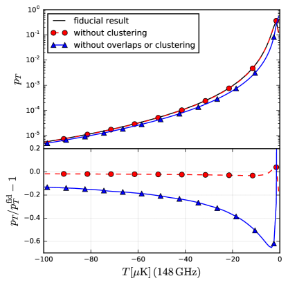
Figure 1: Effects of clustering and overlaps on the tSZ one-point PDF. The fiducial curve (black; including overlaps and clustering) and the result without clustering (red circles) are obtained using the new Fourier-based approach presented in §III, while the result without clustering or overlaps (blue triangles) is calculated using the formalism of H14 as described in §II. The bottom panel presents the fractional difference of the latter two curves with respect to the fiducial curve. For clarity, only selected datapoints are plotted with markers.

IV Comparison to Simulations

We check the validity of our analytic approach by comparing to the results of two different simulation methods. First, we produce “simplified”random maps, in which unclustered halos are randomly distributed on a simulated flat-sky map and assigned Compton-$y$ profiles computed with the B12 pressure profile. We then measure the average tSZ PDF from these maps. By construction, the one-point PDF of our simplified simulations should agree perfectly with our “unclustered” analytic result in Eq. (19), but verifying the agreement is a strong check on details of the implementation, which are nontrivial (see §III.4).

Second, we measure the tSZ PDF from Compton-$y$ maps constructed directly from the cosmological hydrodynamics simulations of B12. The simulated maps in this case only include tSZ signal from halos at $z<1$, and thus in this section we set the upper redshift integration boundary to $z=1$ in our analytic calculations, in order to enable direct comparison with the simulated maps. Note that our fiducial cosmology is identical to that used in B12.

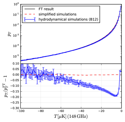
Figure 2: Comparison of our analytic tSZ PDF results to the PDF measured via two sets of simulations. The top panel shows our fiducial analytic result computed via Eq. 27 (black), the PDF measured from “simplified” simulations that neglect halo clustering (dashed red), and the PDF measured from cosmological hydrodynamics simulations (solid blue with error bars). The bottom panel shows the fractional difference of the analytic results with respect to the simulation-derived results. The discrepancy seen with the hydrodynamical simulations is investigated further in Fig. 3, and found to be due to halo mass function differences. Note that we compare the hydrodynamical simulations to the analytic model including clustering, while the simplified simulations are compared to the analytic model without clustering (not plotted in the top panel for clarity). The error bars on the B12 results are estimated from the scatter amongst the simulated maps. Note that in the upper panel the difference between the clustered and unclustered analytic results would be invisible by eye, and thus only one curve has been plotted.

IV.1 Simplified Simulations

The simulations described in this section are produced as follows. We construct individual maps of area $\Omega=10\times 10\,{\rm deg}^{2}$, with square pixels of side-length $3\,{\rm arcsec}$. We then consider discrete, narrow bins in mass and redshift of size $dM\,dz$ centered around $M,z$, for which we compute the average number of such halos in the map via $n(M,z)=\Omega\,dn(M,z)/d\Omega$. For each such mass-redshift bin, we populate the map with $y$-profiles (using the B12 pressure profile), whose number is given by the probability distribution $w(\lceil\!n\!\rceil)=n-\lfloor\!n\!\rfloor$, and $w(\lfloor\!n\!\rfloor)=\lceil\!n\!\rceil-n$. Since this distribution reproduces the correct mean, it is valid to use it to find the average tSZ PDF computed from many maps. We find that sampling the number of halos from the physically more realistic Poisson distribution leads to relatively slow convergence of the average PDF, but we have confirmed that it yields a consistent result with the more rapid approach. Note that we do not include halo clustering in these maps.

Fig. 2 shows the average tSZ PDF computed from 507 simplified simulations (dashed red curve). As the maps do not include clustering of halos, we compare the simulation-derived PDF to the analytic result from §III.2, in which clustering effects are not included (but halo overlaps are). The discrepancy with our analytic result is on average $\approx 0.2\%$ and decreases as more maps are added to the average. This confirms the validity of our analytic formalism, in the limit where halo clustering effects can be neglected.

IV.2 Cosmological Hydrodynamics Simulations

We now compare the results of the full analytic calculation presented in §III.3 (including halo clustering) to measurements of the tSZ PDF from cosmological hydrodynamics simulations. We use Compton-$y$ maps constructed by direct LOS integration (to $z=1$) of randomly rotated and translated simulated volumes from Ref. Battaglia2010 . These are the same simulations from which the B12 pressure profile fitting function was extracted; thus, the comparison here is a direct test of our analytic formalism for the tSZ PDF, with no additional tuning of ICM parameters required. The simulations were performed using the smoothed particle hydrodynamics code GADGET-2, with a custom implementation of a sub-grid prescription for feedback from active galactic nuclei. The pressure profile model extracted from the simulations has subsequently been found to agree with a wide range of tSZ and X-ray measurements (e.g., Sun2011 ; Planck2013stack ; Hajian2013 ; HS2014 ; Greco2015 ; Hilletal2018 ). A full description of the simulations can be found in Ref. Battaglia2010 .

We consider 390 Compton-$y$ maps extracted from the simulations, each of area $\Omega=4.09\times 4.09\,{\rm deg}^{2}$, with square pixels of side-length $6\,{\rm arcsec}$. The average tSZ PDF measured from this suite of $y$-maps is shown in Fig. 2 (blue curve with error bars). As mentioned above, an upper redshift cut at $z=1$ is applied in the construction of the maps, so as to minimize correlations arising from high-redshift objects common to multiple maps. We apply this redshift cut in the analytic calculation in this subsection (and only this subsection) for consistency with the simulated maps.

The agreement in Fig. 2 between the tSZ PDF measured from the hydrodynamical simulations and our analytic result is much worse than the agreement for the simplified simulations seen in the previous subsection. However, this difference can be traced back to the discrepancy between the halo mass function found in B12 and the mass function Tinker2010 used in this work. We explicitly confirm that this halo mass function difference can indeed give rise to discrepancies in the one-point PDF as observed in Fig. 2.

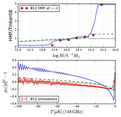
Figure 3: Illustration of the impact of the halo mass function on the one-point PDF. Upper panel: different interpolations of the halo mass function given in B12. The red points are the mass function measured at $z=0$ in B12; the colored curves correspond to various interpolations of these points. Lower panel: corresponding fractional differences to our fiducial result. The colored curves match the same cases in the top panel. The red points with error bars are identical to those in Fig. 2. Modifications of the mass function clearly affect the predicted PDF, and can explain much of the difference between our analytic result and the PDF measured from the hydrodynamical simulations.

In Fig. 3 we show how different interpolations of the halo mass function (HMF) given in B12 (see their Fig. 11) affect the PDF. This is compared to the discrepancy found between our fiducial result and the PDF measured from the B12 simulations. Since only information for redshift $z=0$ is available in Fig. 11 of B12, we take the ratio between the interpolated halo mass function and the fitting function Tinker2008 as constant across redshift. Although this is likely a gross oversimplification, it can be seen from the figure that reasonable interpolations can already reproduce the observed discrepancy very well. We thus conclude that our analytic formalism passes this check, although future comparisons with additional hydrodynamical simulations will also be useful.

V Origin of the Signal

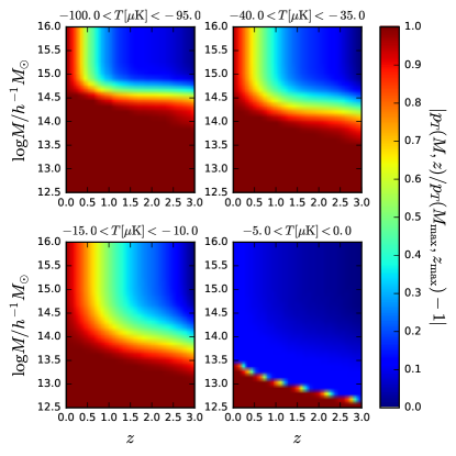
Figure 4: Mass and redshift contributions. We plot the absolute fractional deviation of the PDF in four different temperature bins of width $5\,\mu\rm K$ as a function of the maximum mass and redshift included in the calculation.

We now turn to the different contributions to the PDF. First, we consider cluster mass and redshift. In Fig. 4 we plot the absolute fractional deviation of the PDF as a function of the maximum mass and redshift included in the calculation. These results were obtained using the simplified simulations generated as described in §IV. It should be noted that care must be taken in interpreting these plots, since overlaps can shift part of the contribution from a certain $(M,z)$-bin to higher $|T|$ values. Furthermore, we note that direct comparison with the analogous results given in H14 is not possible, because their results included instrumental noise, non-tSZ foregrounds, and beam convolution.

Regarding the mass contributions, we note two general trends in Fig. 4. First, as $|T|$ increases, the transition region, i.e., the range of relevant masses for the specific temperature bin, gets smaller (ignoring the temperature bin that contains the clear sky fraction for now). At high $|T|$, the PDF in a given temperature bin is dominated by clusters in a narrow mass range. On the other hand, for low $|T|$ a variety of sources contributes. Second, the relevant masses are higher for high $|T|$, which is expected.

Regarding the redshift contributions, the most relevant interval broadens and shifts to larger redshift as $|T|$ decreases. For the temperature bin containing the clear sky fraction the behavior is drastically different, with a very small interval in mass and redshift being the dominant contribution.

Now we consider the effect of the radial cutoff. In our fiducial computation we considered the $y$-profile up to $r_{\rm out}=2\,r_{\rm vir}$. In Fig. 5 we show how the choice of this outer radius affects the PDF. The effect is largest for the low-$|T|$ regime. These temperature bins receive significant contributions from the outskirts of clusters. Furthermore, as discussed above, overlaps have their largest impact on these bins, and reducing the outer radius decreases the amount of overlaps. The clear sky fraction is increased as $r_{\rm out}$ is decreased, which is intuitively clear. We note that the choice of $r_{\rm out}=2\,r_{\rm vir}$ does not correspond to convergence, since there is still a significant discrepancy to the result obtained with $r_{\rm out}=3\,r_{\rm vir}$. However, it is physically not justified to suppose the validity of the pressure profile fitting function up to infinite radius. Physically, the virial shock will lead to a sharp decline in the pressure profile at $r\approx 2-2.5r_{200c}$. Upon convolution with instrumental noise (as described in §VII) the precise choice of radial cutoff becomes irrelevant to the PDF prediction, as the extremely small $y$ values in the outskirts are subsumed into the noise.

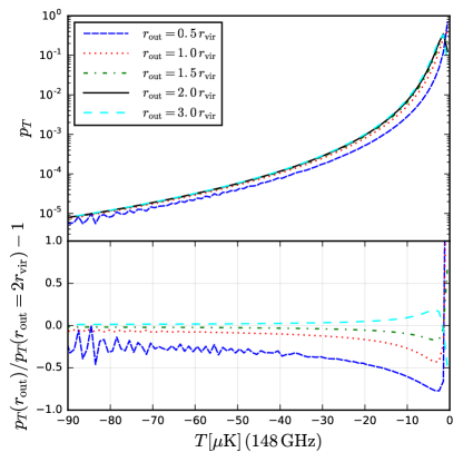
Figure 5: Effect of radial cutoff. The top panel shows the tSZ PDF computed via Eq. 27 with varying choices of the outer radial cutoff of the pressure profile (as labeled). For the curve corresponding to $r_{\rm out}=0.5\,r_{\rm vir}$, the ringing is due to non-convergence of the FT as mentioned earlier. The bottom panel shows the fractional difference with respect to our fiducial choice of $r_{\rm out}=2\,r_{\rm vir}$.

VI Parameter Dependence

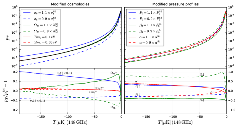
Figure 6: Effect of varying cosmological (left) and ICM pressure profile (right) parameters. For clarity, the residual curves for $\sigma_{8}$ are reduced by a factor of 10. The wiggles at large $|T|$ are due to the angular grid on which the $y$-profiles have been evaluated. Note the different vertical scale in the two residual plots.

We now turn to the dependence of the PDF on cosmological and pressure profile parameters. In Fig. 6 we plot the effect of changing the cosmological parameters $\sigma_{8}$, $\Omega_{\rm M}$, and $\Sigma m_{\nu}$, as well as the pressure profile parameters $P_{0}$, $\beta_{0}$, and $\alpha$ as defined in §II. When considering non-zero neutrino masses we take $N_{\rm eff}=3.046$.

The impact of changing the cosmology is as follows. The neutrino mass sum has its largest effect on high $|T|$ bins, consistent with the fact that it changes the matter power spectrum most on small spatial scales, which here leads to a suppression in the number of clusters (however, to hold $\sigma_{8}$ fixed, the initial scalar amplitude $A_{s}$ must be increased, thus leading to an overall increase in the number of clusters; this is simply an artifact of this choice of cosmological parameters). The impact of changing $\sigma_{8}$ is similar, yielding a mild degeneracy with $\Sigma m_{\nu}$. On the other hand, changing $\Omega_{\rm M}$ has largest impact on low $|T|$ bins. Thus, degeneracy between $\sigma_{8}$ and $\Omega_{\rm M}$ could be broken by a measurement of the tSZ PDF over a sufficiently large $|T|$ range.

The pressure profile parameters affect the PDF as follows. $P_{0}$ changes the PDF relatively constantly across temperature, which is explained by the fact that it is an overall normalization of the pressure profile. Changing the logarithmic slope at large radii, $\beta_{0}$, produces a similar effect, although with the opposite sign. Increasing the logarithmic slope at intermediate radii, $\alpha$, decreases the PDF in low $|T|$ bins and increases it in large $|T|$ bins.

VII Including noise and foregrounds

Here we consider a representative upcoming CMB experiment and demonstrate the necessity of our improved analytic approach for modeling the tSZ PDF sufficiently accurately to perform unbiased inference from this observable. In lieu of full parameter forecasts, which require treatment of the covariance matrix and likelihood function, we simply compute the predictions from our full analytic model (Eq. 27) and from the H14 model (Eq. 5), and compare these to predicted error bars on a measurement of the tSZ PDF.

Specifically, we consider a measurement with the Simons Observatory (SO), which will cover $f_{\rm sky}=0.4$ with six frequency channels, reaching a depth and resolution at 145 GHz of $6\,\mu$K-arcmin and FWHM = 1.4 arcmin, respectively SO2018 . We include the effects of non-tSZ foregrounds via the post-component-separation Compton-$y$ noise power spectra that are publicly available via the SO Collaboration. In particular, we use the $y$ noise power spectrum, $N_{\ell}^{yy}$, derived via the “standard internal linear combination”, without additional deprojection constraints (see SO2018 for further details about the foreground modeling and component separation). In practice, deprojection options will have to be explored in the foreground cleaning as well, but this is beyond the scope of our work here.

We construct a Wiener filter to optimally weight the harmonic-space tSZ signal via

$$F_{\ell}=C_{\ell}^{yy}/(C_{\ell}^{yy}+N_{\ell}^{yy})\,,$$ (28)

where $C_{\ell}^{yy}$ is the tSZ power spectrum, which we compute using the fiducial model of Hill-Pajer2013 . The filter is smoothly tapered to zero at the boundaries of the multipole range provided in the $N_{\ell}^{yy}$ data file ($\ell_{\rm min}\approx 40$ and $\ell_{\rm max}\approx 8000$). We apply this filter to the $y$-profiles of all halos in our analytic calculation, which captures the suppression of modes lost due to foregrounds and noise. Note that the multifrequency information of SO (and Planck, which is also used) allows large-scale tSZ modes to be included (because the CMB can be removed using spectral information), which were lost due to CMB “noise” in the single-frequency ACT analysis of H14. Thus the filter extends to lower multipoles than in H14 (which used a filter originally constructed in Wilson2012 ).

After calculating the analytic prediction for the filtered tSZ PDF, we convolve the result with a Gaussian noise (+residual foreground) PDF, whose variance is computed via

$$\sigma_{yy}^{2}=\sum_{\ell}\frac{2\ell+1}{4\pi}N_{\ell}^{yy}F_{\ell}^{2}p_{\ell}^{2}\,,$$ (29)

where $p_{\ell}$ is the pixel window function (here assumed to be 0.5 arcmin circular pixels, although this has negligible effect). We then rescale the results from Compton-$y$ to 148 GHz temperature to match those shown elsewhere in the paper (although the application of the filter and noise convolution mean the temperature values are not comparable to those in earlier plots). We bin the results into bins of width $5\,\mu$K.

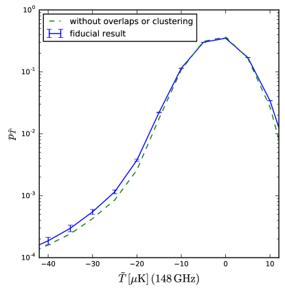
Figure 7: Difference between our fiducial analytic result (Eq. 27; solid blue) and the result neglecting overlaps and halo clustering (i.e., the H14 model; dashed green), with noise and non-tSZ foregrounds included. The latter are modeled and propagated through multifrequency component separation via the publicly available Simons Observatory Compton-$y$ noise power spectra. Note that a Wiener filter has been applied to the $\tilde{T}$ field here, as denoted by the tilde, and hence the values are not directly comparable to those in other figures. The convolution with noise and residual foregrounds is responsible for the non-zero PDF values for $\tilde{T}>0$. It is clear that the earlier H14 model is not sufficiently accurate for SO analysis; the difference between our improved model and the previous model is larger than the error bars in essentially all bins shown.

The results are shown in Fig. 7. The solid blue curve shows the prediction from the FT-based formalism developed in this paper (Eq. 27). The dashed green curve shows the prediction from the H14 model (Eq. 5). The error bars shown on the blue curve are computed using the diagonal elements of the covariance matrix $C_{ij}$ estimated from the simplified simulations described in §IV.1, but with Poisson distributed cluster numbers, rather than the modified distribution described earlier (which achieved faster convergence at the expense of only capturing the mean correctly), so that the variance is correctly captured. Specifically, we compute the error on the value of the PDF in the $i$th bin as

$$\sigma_{i}=\sqrt{\frac{f_{\rm sky}^{\rm maps}}{f_{\rm sky}^{\rm survey}}}\times\frac{d_{\rm pixel}^{\rm survey}}{d_{\rm pixel}^{\rm maps}}\times\sqrt{C_{ii}},$$ (30)

where $f_{\rm sky}$ are the sky fractions and $d_{\rm pixel}$ the pixel side lengths. We take $f_{\rm sky}^{\rm SO}=0.4$ and $d_{\rm pixel}^{\rm SO}=0.5\,{\rm arcmin}$; the simulation parameters are $f_{\rm sky}^{\rm maps}=6.21\times 10^{-3}$ and $d_{\rm pixel}^{\rm maps}=0.1\,{\rm arcmin}$. For a survey with the properties described above, the difference between the no-overlaps case and our fiducial result is considerably larger than the errors for essentially all bins plotted. We note that the error bars themselves should not be taken at face value, because significant bin-to-bin correlations exist as discussed in H14. Nevertheless, we conclude that if the earlier model of H14 were used in an analysis of the tSZ PDF from SO, cosmological and ICM parameter inference would clearly be biased. With our accurate model in hand, we plan to pursue full parameter forecasts for ongoing and upcoming CMB experiments in future work.

VIII Outlook

In this paper we have presented a new analytic model for the tSZ one-point PDF, building upon and substantially improving the model first developed in H14. In particular, by working in Fourier conjugate space, we have shown how to account for effects due to overlaps in the tSZ profiles of halos on the sky, as well as contributions due to the clustering of halos (which arise because of the LOS projection). For the tSZ PDF, the effects due to overlaps are non-negligible, but the clustering effects are rather small. We have verified the accuracy of the model via comparison to numerical simulations, both simplified simulations containing randomly distributed clusters and full-scale cosmological hydrodynamics simulations. However, issues related to the halo mass function in the latter simulations rendered a precise test of the clustering effects challenging; future simulation comparisons will thus be useful. Finally, we have demonstrated that the use of this more accurate analytic model will be necessary in analyses of the tSZ PDF in upcoming, high-sensitivity CMB data sets.

We anticipate a number of interesting next steps in this line of research. An obvious first step is to compute the covariance matrix in this formalism and the likelihood function associated with the PDF observable. Given the challenges observed in this context in H14, it may be useful to pursue novel approaches such as likelihood-free inference (although this could render the analytic model redundant) Alsing2018 . We expect that the forecast cosmological constraints using the tSZ PDF will significantly improve upon those for the tSZ power spectrum alone (e.g., as presented in Ref. SO2018 ). An optimal combination with constraints from individually detected clusters is clearly also a pressing issue, and will lead to further improvements.

Beyond the tSZ signal, the formalism developed here likely has applications to other cosmological fields. An obvious candidate is the one-point PDF of the weak lensing convergence field, which has already been investigated in simulations Liu2016 ; Patton2017 ; Liu-Madhavacheril2018 . We expect that the clustering effects computed in this paper will be more important for this application than for the tSZ field. In addition, further development to treat negative-convergence regions (voids) will be necessary. Nevertheless, a full, non-perturbative model for the one-point PDF of the projected density field is clearly a goal worth pursuing.

Appendix A Equivalence to Formalism of H14

In this appendix we show that our analytic model is equivalent to the formalism used in H14 under the assumption that no overlaps occur. Denote $\int dM\int dz(\chi^{2}/H)(dn/dM)$ by $\int_{M,z}$ for brevity. The arguments $M$ and $z$ are understood for $y_{0}(M,z,\theta)$, etc. Integrating Eq. (16) (which is equivalent to a first order expansion of Eq. 19) over mass and redshift, we obtain

$$\tilde{P}(\lambda)=1+\int_{M,z}\,\int d\theta\,2\pi\theta(\mathrm{e}^{i\lambda y_{0}(\theta)}-1).$$

The one-point PDF in $y$-space is given by:

$$P(y) =\delta(y)+\int_{M,z}\int d\theta\,\theta\int d\lambda\,(\mathrm{e}^{i\lambda[y_{0}(\theta)-y]}-\mathrm{e}^{-i\lambda y})$$

$$=\delta(y)+\int_{M,z}\left[-2\pi\delta(y)\frac{\theta_{\rm max}^{2}}{2}+2\pi\frac{\theta_{0}(y)}{|dy/d\theta_{0}|}\right],$$

where we denote the inverse function to $y_{0}(\theta)$ by $\theta_{0}(y)$. The PDF binned into $y_{i}\leq y\leq y_{i+1}$ is then found as

$$p_{i} =\int_{y_{i}}^{y_{i+1}}dy\,P(y)$$

$$=\delta_{i}\,\left(1-\int_{M,z}\pi\theta_{\rm max}^{2}\right)+\int_{M,z}2\pi\int_{y_{i}}^{y_{i+1}}dy\,\left|\frac{d\theta_{0}}{dy}\right|\theta_{0}(y)$$

$$=\delta_{i}\,(1-F_{\rm clust})+\int_{M,z}\pi\left[\theta_{0}^{2}(y_{i+1})-\theta_{0}^{2}(y_{i})\right]$$ (31)

where $\delta_{i}$ equals one if $y=0$ is contained in the integration interval and zero otherwise. $\theta_{\rm max}=\theta_{\rm max}(M,z)$ corresponds to the radial cutoff, so that $1-F_{\rm clust}$ is the clear-sky fraction. This is the expression used in H14, i.e., Eq. (5) presented earlier.

References

- (1) Planck Collaboration et al., arXiv e-prints , arXiv:1807.06209 (2018), 1807.06209.
- (2) Planck Collaboration et al., A&A594, A17 (2016), 1502.01592.
- (3) G. Hinshaw et al., The Astrophysical Journal Supplement Series 208, 19 (2013), 1212.5226.
- (4) J. C. Hill et al., ArXiv e-prints (2014), 1411.8004.
- (5) Y. B. Zeldovich and R. A. Sunyaev, Ap&SS4, 301 (1969).
- (6) R. A. Sunyaev and Y. B. Zeldovich, Ap&SS7, 3 (1970).
- (7) M. Hasselfield et al., Journal of Cosmology and Astro-Particle Physics 2013, 008 (2013), 1301.0816.
- (8) Planck Collaboration et al., A&A594, A24 (2016), 1502.01597.
- (9) S. Bocquet et al., arXiv e-prints , arXiv:1812.01679 (2018), 1812.01679.
- (10) E. Komatsu and U. Seljak, MNRAS336, 1256 (2002), astro-ph/0205468.
- (11) J. C. Hill and E. Pajer, Phys. Rev. D88, 063526 (2013), 1303.4726.
- (12) I. G. McCarthy, A. M. C. Le Brun, J. Schaye, and G. P. Holder, MNRAS440, 3645 (2014), 1312.5341.
- (13) B. Horowitz and U. Seljak, MNRAS469, 394 (2017), 1609.01850.
- (14) J. L. Sievers et al., Journal of Cosmology and Astro-Particle Physics 2013, 060 (2013), 1301.0824.
- (15) E. M. George et al., ApJ799, 177 (2015), 1408.3161.
- (16) Planck Collaboration et al., A&A571, A21 (2014), 1303.5081.
- (17) Planck Collaboration et al., A&A594, A22 (2016), 1502.01596.
- (18) M. J. Wilson et al., Phys. Rev. D86, 122005 (2012), 1203.6633.
- (19) S. Bhattacharya, D. Nagai, L. Shaw, T. Crawford, and G. P. Holder, ApJ760, 5 (2012), 1203.6368.
- (20) T. M. Crawford et al., ApJ784, 143 (2014), 1303.3535.
- (21) J. C. Hill and D. N. Spergel, J. Cosmology Astropart. Phys2, 030 (2014), 1312.4525.
- (22) L. Van Waerbeke, G. Hinshaw, and N. Murray, Phys. Rev. D89, 023508 (2014), 1310.5721.
- (23) A. Hojjati et al., MNRAS471, 1565 (2017), 1608.07581.
- (24) J. C. Hill and B. D. Sherwin, Phys. Rev. D87, 023527 (2013), 1205.5794.
- (25) E. Komatsu and T. Kitayama, ApJ526, L1 (1999), astro-ph/9908087.
- (26) S. W. Henderson et al., Journal of Low Temperature Physics 184, 772 (2016), 1510.02809.
- (27) B. A. Benson et al., SPT-3G: a next-generation cosmic microwave background polarization experiment on the South Pole telescope, in Millimeter, Submillimeter, and Far-Infrared Detectors and Instrumentation for Astronomy VII, , Society of Photo-Optical Instrumentation Engineers (SPIE) Conference Series Vol. 9153, p. 91531P, 2014, 1407.2973.
- (28) The Simons Observatory Collaboration et al., arXiv e-prints , arXiv:1808.07445 (2018), 1808.07445.
- (29) The Simons Observatory Collaboration et al., arXiv e-prints , arXiv:1808.07445 (2018), 1808.07445.
- (30) J. Liu et al., Phys. Rev. D94, 103501 (2016), 1608.03169.
- (31) K. Patton et al., MNRAS472, 439 (2017), 1611.01486.
- (32) J. Liu and M. S. Madhavacheril, arXiv e-prints , arXiv:1809.10747 (2018), 1809.10747.
- (33) S. Nozawa, N. Itoh, Y. Suda, and Y. Ohhata, Nuovo Cimento B Serie 121, 487 (2006), astro-ph/0507466.
- (34) J. L. Tinker et al., ApJ724, 878 (2010), 1001.3162.
- (35) N. Battaglia, J. R. Bond, C. Pfrommer, and J. L. Sievers, ApJ758, 75 (2012), 1109.3711.
- (36) J. F. Navarro, C. S. Frenk, and S. D. M. White, ApJ490, 493 (1997), astro-ph/9611107.
- (37) A. R. Duffy, J. Schaye, S. T. Kay, and C. Dalla Vecchia, MNRAS390, L64 (2008), 0804.2486.
- (38) B. Diemer, arXiv e-prints (2017), 1712.04512.
- (39) G. L. Bryan and M. L. Norman, ApJ495, 80 (1998), astro-ph/9710107.
- (40) P. A. G. Scheuer, Proceedings of the Cambridge Philosophical Society 53, 764 (1957).
- (41) J. J. Condon, ApJ188, 279 (1974).
- (42) P. Zhang and R. K. Sheth, ApJ671, 14 (2007), astro-ph/0701879.
- (43) A. Lewis, A. Challinor, and A. Lasenby, ApJ538, 473 (2000), astro-ph/9911177.
- (44) N. Battaglia, J. R. Bond, C. Pfrommer, J. L. Sievers, and D. Sijacki, ApJ725, 91 (2010), 1003.4256.
- (45) M. Sun et al., ApJ727, L49 (2011), 1012.0312.
- (46) Planck Collaboration et al., A&A550, A131 (2013), 1207.4061.
- (47) A. Hajian et al., J. Cosmology Astropart. Phys11, 064 (2013), 1309.3282.
- (48) J. P. Greco, J. C. Hill, D. N. Spergel, and N. Battaglia, ApJ808, 151 (2015), 1409.6747.
- (49) J. C. Hill, E. J. Baxter, A. Lidz, J. P. Greco, and B. Jain, Phys. Rev. D97, 083501 (2018), 1706.03753.
- (50) J. Tinker et al., ApJ688, 709 (2008), 0803.2706.
- (51) J. Alsing, B. Wandelt, and S. Feeney, MNRAS477, 2874 (2018), 1801.01497.