Reduced Density-Matrix Approach to Strong Matter-Photon Interaction

Abstract

We present a first-principles approach to electronic many-body systems strongly coupled to cavity modes in terms of matter-photon one-body reduced density matrices. The theory is fundamentally non-perturbative and thus captures not only the effects of correlated electronic systems but accounts also for strong interactions between matter and photon degrees of freedom. We do so by introducing a higher-dimensional auxiliary system that maps the coupled fermion-boson system to a dressed fermionic problem. This reformulation allows us to overcome many fundamental challenges of density-matrix theory in the context of coupled fermion-boson systems and we can employ conventional reduced density-matrix functional theory developed for purely fermionic systems. We provide results for one-dimensional model systems in real space and show that simple density-matrix approximations are accurate from the weak to the deep-strong coupling regime. This justifies the application of our method to systems that are too complex for exact calculations and we present first results, which show that the influence of the photon field depends sensitively on the details of the electronic structure.

Center for Computational Quantum Physics (CCQ), Flatiron Institute, 162 Fifth Avenue, New York NY 10010, USA

Experiments performed in the last decades (see, e.g., Refs. 1, 2) have made accessible the strong and ultra-strong interaction regime between matter degrees of freedom and the quantized modes of optical cavities, which allows for the study of many new phenomena including modification of chemical reaction rates ^{4, 5}, interacting photons in quantum non-linear media ⁶ or super-radiance of atoms in a photonic trap ⁷. At the same time it creates opportunities such as the modification of energy-transfer pathways within photosynthetic organisms ⁸, an increase of conductivity in organic semiconductors hybridized with the vacuum field ⁹ or the generation of long-distance molecular interactions that, for example, allow for energy transfer way beyond the short-range dipole-dipole mediated transfer (Förster theory) ¹⁰. All these phenomena are related by the emergence of hybrid light-matter quasi-particle states, called polaritons, that determine the properties of the respective coupled electron-photon system. The physics of these exotic states can be understood impressively well by model systems of Dicke-type ¹¹, meaning several few-level systems coupled to some photon modes ³. Many experimentally found features of the (ultra-)strong coupling regime could be described ^{12, 13, 14, 15, 16} and much exciting new physics was predicted ^{17, 18, 19, 20, 21} using such models. This article focuses on the influence of (ultra-)strong coupling on the ground state of light-matter systems, a topic on which considerably less literature exists. Only recently, polaritonic ground states, which are believed to be fundamental for the understanding of polaritonic chemistry ¹, have been started to be investigated in more detail ^{22, 3}. However, limits and difficulties of few level-approximations have been pointed out ^{23, 24, 25, 26, 27, 28} and recently, new models have been used to investigate polaritonic chemistry ^{29, 15, 30, 31, 32, 33, 34, 35, 28, 36, 37, 38, 39, 40, 41}. Still, many questions remain open, especially whether the collective (ultra-)strong coupling, predicted by the Dicke-model can actually modify ground state properties of single molecules^{17, 42}. Another example is the ongoing discussion on the theoretical understanding of super-radiance ^{43, 24}. These debates suggest that there is a need for new theoretical tools that treat matter and photons at the same level of theory ^{35, 27, 28}. Up to now, standard theoretical modelling treats in detail either the photons or the matter, which becomes insufficient when the matter and photon degrees of freedom are equally important ²⁷. We present in this paper further evidence that the impact of the light-matter interaction on the matter is far from trivial and can change from system to system.

However, the full quantum-mechanical description of just the electronic degrees of freedom is already computationally very challenging due to the exponential scaling of the wave function. Instead, reformulations of the many-body problem in terms of reduced quantities like the electron density ^{44, 45} or the Green’s function ^{46, 47, 48} have been shown to provide accurate results for relatively low computational costs. Thus, working with reduced quantities seems to be a natural choice also for coupled light-matter systems⁴⁹. Recently, quantum-electrodynamical density-functional theory (QEDFT) was introduced as an extension to pure electronic density-functional theory (DFT) ^{50, 51, 52, 53}. First calculations showed the feasibility of QEDFT ^{54, 55} leading to the possibility to perform full first-principles calculations of real molecules coupled to cavity modes ^{56, 57}. However, standard approximations in DFT (usually based on a non-interacting auxiliary Kohn-Sham system) become inaccurate if applied to strongly-correlated systems. This is very well studied in terms of the strong-correlation regime in electronic systems ⁵⁸ and also observed for the existing QEDFT functionals that approximate the electron-photon interaction ⁵⁶. Consequently, to study novel effects arising in the ultra-strong ⁵⁹ or deep-strong coupling regime ⁶⁰ of light and matter from first principles, i.e., without resorting to simplified few-level systems, one needs to develop new functionals for the combined matter-photon systems or explore alternative many-body methods.

Reduced density-matrix functional theory (RDMFT) is such a method. RDMFT is based on the electronic one-body reduced density matrix (1RDM) instead of the electronic density (as in DFT) as its basic functional variable ⁶¹. Similarly to DFT, approximations are necessary in RDMFT as it is not known how to express explicitly all expectation values of operators in terms of the 1RDM. Simple approximations within this approach ⁶² have proven very efficient in dealing with difficult electronic structure problems like the correct qualitative description of a dissociating molecule ⁶³ or the prediction of the Mott-insulating phase of certain strongly-correlated solids ⁶⁴. Thus, it seems worth to explore how RDMFT performs in describing also the strong interaction between molecular systems and cavity modes.

Figure 1: Typical setting of a cavity experiment. A matter system (here represented by a diatomic molecule) is put inside an optical cavity that enhances specific modes of the electromagnetic field (here represented by the lowest cavity mode, but in principle many modes can become important.) By that, the coupling between the matter system and the light modes can be considerably enhanced with respect to the free space. The dipole of the molecule should to be aligned with the polarization of the enhanced mode and its position is assumed at the field maximum. Note that in principle also higher multipole moments can become important.

Specifically, we will discuss in this work the properties of coupled light-matter systems in a setting that resembles typical cavity experiments (see Fig. 1.) It turns out that transferring RDMFT to such systems involves overcoming additional difficulties in contrast to the DFT framework. The reason behind this are the conditions under which the corresponding reduced density matrices (RDMs) (which will be purely electronic, purely photonic and coupled) connect to the original wave function, which is crucial to construct a well-defined reduced density-matrix framework. Already for the purely electronic system the conditions under which such a connection exists (known as N-representability conditions) are not trivial ^{65, 66, 67}. For RDMs in matter-photon systems, these conditions are entirely unexplored. Nevertheless, we manage to overcome this difficulty by mapping the original system to a higher-dimensional auxiliary system that allows for an effective description of the problem by fermions. Hence, the corresponding RDMs connect to the auxiliary wave functions under N-representability conditions of fermionic systems. Despite being fermions, the newly introduced quasi-particles will depend on electronic and bosonic degrees of freedom. This construction was recently introduced by some of the authors in Ref. 68 and used to construct a DFT scheme specifically for the strong-coupling regime of light-matter systems. In the auxiliary system, the Hamiltonian consists of only 1- and 2-body terms for the new quasi-particles, thus it has the same structure as the conventional electronic Hamiltonian for molecular systems, which allows us to apply electronic RDMFT theory without major modifications. We will present some results for model systems with the simplest known RDMFT functional, the Müller functional ⁶², and show that this dressed RDMFT is accurate from the weak to the strong-coupling regime. Then, we will present two examples highlighting that how matter reacts to the interaction with photons depends strongly on the system. For instance, for the same coupling strength, the repulsion between the particles can be locally suppressed in one system but enhanced in another. We finish with commenting on some open issues and challenges for future applications.

This article is structured as follows. First, we explain the physical setting of an electronic system in a cavity in Sec. Physical Setting. In Sec. Reduced Density Matrices for coupled light-matter systems, we discuss the RDMs that appear in the ground-state energy expression of the coupled light-matter system. We will explain the difficulties that are introduced by the coupling between fermions and bosons and having non-particle-conserving terms. In Sec. The “fermionization” of matter-photon systems, we introduce the higher-dimensional auxiliary system which will allow us to avoid most of the aforementioned difficulties. We show how to construct a proper RDMFT framework in this system in Sec. Dressed Reduced Density-Matrix Functional Theory, explain our numerical implementation in Sec. Numerical Implementation, and present the numerical results in Sec. Numerical Results. We finish with discussing possibilities as well as challenges of dressed RDMFT in Sec. Conclusion.

Physical Setting

To describe weak and strong matter-photon interaction, it is necessary to go beyond typical quantum-chemistry or solid-state physics theories that describe electrons in a local potential interacting via Coulomb interaction and being perturbed by a classical external electromagnetic field. Instead, we need to treat explicitly the quantum nature of light and the back-reaction between electrons and electromagnetic field excitations (photons) ³⁵. Therefore, the framework of quantum electrodynamics (QED) needs to be employed. However, we do not want to treat QED in its full complexity but will apply some well-established approximations (see Ref. 35 for a detailed discussion.) First, we apply the Born-Oppenheimer approximation and treat the nuclei as fixed classical particles. Second, we work in the non-relativistic limit, which for the typical energy scales of molecules and their low-energy excitations is usually sufficient. Third, we assume that the wavelength $\lambda$ of the relevant electromagnetic modes is much larger than the spatial extension $d$ of the electronic system ($\lambda\gg d$) such that the dipole approximation (here in the Coulomb gauge) is valid ^{69, 70}. In the case of the dipole approximation, where every photon mode couples to all Fourier components of the charge current of the electronic subsystem ^{52, 53}, an effective description with only a few modes is usually sufficient. The continuum of modes is then effectively taken into account by using instead of the bare mass the physical mass of the electrons ^{57, 27}. Since we focus on equilibrium situations, the openness of the cavity can be neglected.

Therefore, the basic Hamiltonian that we use to describe strongly-coupled light-matter systems reads (we use atomic units throughout)

$$\hat{H} =\sum_{k=1}^{N}\left[-\tfrac{1}{2}\nabla_{\mathbf{r}_{k}}^{2}+v(\mathbf{r}_{k})\right]+\tfrac{1}{2}\sum_{k\neq l}w(\mathbf{r}_{k},\mathbf{r}_{l})+\tfrac{1}{2}\sum_{\alpha=1}^{M}\left[-\tfrac{\partial^{2}}{\partial p_{\alpha}^{2}}+\left(\omega_{\alpha}p_{\alpha}-\bm{\lambda}_{\alpha}\cdot\sum_{k=1}^{N}\mathbf{r}_{k}\right)^{2}\,\right].$$ (1)

Here the first two sums on the right-hand side correspond to the usual electronic many-body Hamiltonian $\hat{H}_{e}=\hat{T}+\hat{V}+\hat{W}$, used to describe the uncoupled matter system consisting of $N$ electrons in an external potential $v(\mathbf{r})$ interacting via the Coulomb repulsion $w(\mathbf{r},\mathbf{r}^{\prime})$. The third sum describes $M$ photon modes, that are characterized by their elongation $p_{\alpha}$, frequency $\omega_{\alpha}$ and polarization vectors $\bm{\lambda}_{\alpha}$. The polarization vectors include already the effective coupling strength $g_{\alpha}=|\bm{\lambda}_{\alpha}|\sqrt{\frac{\omega_{\alpha}}{2}}$³⁵ and couple to the total dipole $\hat{\mathbf{D}}=\sum_{k=1}^{N}\mathbf{r}_{k}$ of the electronic system. The sum can be decomposed in a purely photonic part $\hat{H}_{ph}=\sum_{\alpha=1}^{M}\left(-\tfrac{1}{2}\tfrac{\partial^{2}}{\partial p_{\alpha}^{2}}+\tfrac{\omega_{\alpha}^{2}}{2}p_{\alpha}^{2}\right)$, the dipole self-interaction $\hat{H}_{d}=\sum_{\alpha=1}^{M}\tfrac{1}{2}\left(\bm{\lambda}_{\alpha}\cdot\hat{\mathbf{D}}\right)^{2}$, which we split again for later convenience in its one-body $\hat{H}_{d}^{(1)}=\sum_{\alpha=1}^{M}\sum_{k=1}^{N}\tfrac{1}{2}(\bm{\lambda}_{\alpha}\cdot\mathbf{r}_{k})^{2}$ and two-body part $\hat{H}_{d}^{(2)}=\sum_{\alpha=1}^{M}\sum_{k\neq l}\tfrac{1}{2}(\bm{\lambda}_{\alpha}\cdot\mathbf{r}_{k})(\bm{\lambda}_{\alpha}\cdot\mathbf{r}_{l})$, and the bilinear interaction $\hat{H}_{I}=-\sum_{\alpha=1}^{M}\omega_{\alpha}p_{\alpha}\bm{\lambda}_{\alpha}\cdot\hat{\mathbf{D}}$. Some comments on this Hamiltonian are appropriate. Since we work in Coulomb gauge, the dipole-self energy term arises only for the transversal but not for the longitudinal part of the field⁷¹. However, if we assume a cavity then the Coulomb interaction is modified⁷². We can easily incorporate this into our framework since $w(\mathbf{r},\mathbf{r}^{\prime})$ is completely at our disposal and we do not rely on any kind of Coulomb approximation. Thus, we can also treat the influence of e.g., a plasmonic environment⁷³.

The ground-state wave function of Eq. (1) is a function of $4N+M$ coordinates

$$\Psi(\mathbf{r}_{1}\sigma_{1},...,\mathbf{r}_{N}\sigma_{N};p_{1},...,p_{M}),$$ (2)

where $\sigma_{k}$ are the electronic spin degrees of freedom. The wave function $\Psi$ is as usual anti-symmetric with respect to the exchange of any two electron coordinates $\mathbf{r}_{j}\sigma_{j}\leftrightarrow\mathbf{r}_{k}\sigma_{k}$, and also depends on $M$ photon-mode displacement coordinates $p_{\alpha}$.

At this point, we want to remind the reader that there is no fundamental symmetry with respect to the exchange of two displacement coordinates $p_{\alpha}$ with $p_{\beta}$. The bosonic symmetry instead refers to the exchange of mode excitations, which are interpreted as photons in the number-state representation. To see this, we first use the ladder operators $\hat{a}_{\alpha}=\sqrt{\tfrac{\omega_{\alpha}}{2}}(p_{\alpha}-\tfrac{1}{\omega_{\alpha}}\tfrac{\partial}{\partial p_{\alpha}})$ and $\hat{a}^{+}_{\alpha}=\sqrt{\tfrac{\omega_{\alpha}}{2}}(p_{\alpha}+\tfrac{1}{\omega_{\alpha}}\tfrac{\partial}{\partial p_{\alpha}})$ to represent the sum of harmonic Hamiltonians, i.e.,

$$\hat{H}_{ph}=\sum_{\alpha=1}^{M}\omega_{\alpha}\left(\hat{a}_{\alpha}^{+}\hat{a}_{\alpha}^{\vphantom{+}}+\tfrac{1}{2}\right).$$ (3)

Eigenstates of the individual $\hat{a}_{\alpha}^{+}\hat{a}_{\alpha}$ in the above representation are given by multiple applications of creation operators to the vacuum state $\ket{0}$, i.e., $\ket{\varphi^{n}_{\alpha}}=(\hat{a}^{+}_{\alpha})^{n}\ket{0}$. These eigenstates are connected to the displacement representation by $\varphi^{n}_{\alpha}(p_{\alpha})=\braket{p_{\alpha}}{\varphi^{n}_{\alpha}}=\braket{p_{\alpha}}{(\hat{a}^{+}_{\alpha})^{n}}{0}$. We can then express an $M$-mode eigenfunction as $\phi_{n_{1},...,n_{M}}(p_{1},...,p_{M})=\braket{p_{1}...p_{M}}{\phi_{n_{1},...,n_{M}}}=\bra{p_{1}...p_{M}}\hat{a}^{+}_{1})^{n_{1}}...$ $(\hat{a}^{+}_{M})^{n_{M}}\ket{0}$. In this form it becomes clear that a multi-mode eigenstate $\ket{\phi_{n_{1},...,n_{M}}}$ can be considered to consist of $N_{b}=n_{1}+...+n_{M}$ photons (mode excitations.) We can associate every such multi-mode eigenstate with a specific photon-number sector, i.e., the zero-photon sector is merely one-dimensional and corresponds to $\ket{\phi_{0_{1},...,0_{M}}}\equiv\ket{0}$, the single-photon sector is $M$-dimensional and corresponds to the span of $\hat{a}^{+}_{\alpha}\ket{0}\equiv\ket{\alpha}$ for all $\alpha$ and so on. For the multi-photon sectors we see due to the commutation relations of the ladder operators the bosonic exchange symmetry appearing, e.g., $\hat{a}^{+}_{\alpha_{1}}\hat{a}^{+}_{\alpha_{2}}\ket{0}=\hat{a}^{+}_{\alpha_{2}}\hat{a}^{+}_{\alpha_{1}}\ket{0}\equiv\ket{\alpha_{1},\alpha_{2}}$ for $\alpha_{1},\alpha_{2}\in\{1,...,M\}$. It is no accident that the bosonic symmetry becomes explicit in this representation since the different modes $\alpha$ determine how the photon wave functions looks like in real space (see also the discussion in App. LABEL:app:symmetry_photon.) A general photon state can therefore be represented by a sum over all photon-number sectors as $\ket{\Phi}=\sum_{n=0}^{\infty}\left(\tfrac{1}{\sqrt{n!}}\sum_{\alpha_{1},...,\alpha_{n}=1}^{M}\tilde{\Phi}(\alpha_{1},...,\alpha_{n})\ket{\alpha_{1},...,\alpha_{n}}\right)$.

Reduced Density Matrices for coupled light-matter systems

$\Psi(\mathbf{r}_{1}\sigma_{1},...,\mathbf{r}_{N}\sigma_{N};p_{1},...,p_{M})$ - electron-photon many-body state $\psi_{e}(\mathbf{r}_{1}\sigma_{1},...,\mathbf{r}_{N}\sigma_{N})$ - purely electronic many-body state $\psi_{b}(\alpha_{1},...,\alpha_{N_{b}})$ - photonic many-body state in mode representation with fixed particle number $\Phi(\alpha_{1},\alpha_{2},...)$ - photonic many-body state in Fock space $\phi_{e}^{i}(\mathbf{r})/\phi_{b}^{i}(\alpha)$ - electronic/photonic natural orbital

Table 1: To ease reading, we highlight the different physical wave functions and the corresponding symbols that appear in this section.

Having introduced our system of interest, we now want to discuss how to find its ground state. A ground state (if it exists) is defined as the state (possibly degenerate) that has the lowest energy expectation value

$$E_{0}[\Psi]=\inf_{\Psi}\braket{\Psi}{\hat{H}\Psi}.$$ (4)

This is the classical formulation of the variational principle due to Ritz and is well-defined for every Hamiltonian that is bounded from below. While well-known, Eq. (4) has the disadvantage that in practice the minimization has to be performed over an enormous configuration space that is spanned by all possible many-body wave functions. A possible reduction of computational complexity presents itself by the fact that the full wave function is usually not necessary to compute the energy expectation value but typically only reduced quantities are sufficient. Varying instead over the space of reduced objects makes the minimization simpler. For instance, in the case of an electronic many-body state $\psi_{e}(\mathbf{r}_{1}\sigma_{1},...,\mathbf{r}_{N}\sigma_{N})$ of $N$ electrons (see Tab. 1), the expectation value of a general (non-local) $q$-body operator $\hat{O}(\mathbf{r}_{1},...\mathbf{r}_{q};\mathbf{r}_{1}^{\prime},...\mathbf{r}_{q}^{\prime})$, which is given by $O=\braket{\psi_{e}}{\hat{O}\psi_{e}}$, can be determined via the electronic (spin-summed) $q$-body RDM ($q$RDM)

$$\Gamma_{e}^{(q)} (\mathbf{r}_{1},...,\mathbf{r}_{q};\mathbf{r}_{1}^{\prime},...,\mathbf{r}_{q}^{\prime})=\tfrac{N!}{(N-q)!}\sum_{\sigma_{1},...,\sigma_{N}}\int\mathrm{d}^{3(N-q)}r$$ (5)

$$\psi_{e}^{*}(\mathbf{r}_{1}^{\prime}\sigma_{1},...,\mathbf{r}_{q}^{\prime}\sigma_{q},\mathbf{r}_{q+1}\sigma_{q+1},...,\mathbf{r}_{N}\sigma_{N})\psi_{e}(\mathbf{r}_{1}\sigma_{1},...,\mathbf{r}_{q}\sigma_{q},\mathbf{r}_{q+1}\sigma_{q+1},...,\mathbf{r}_{N}\sigma_{N}).$$

For instance, the well-known electronic 1RDM, that we denote in the following by $\gamma_{e}(\mathbf{r},\mathbf{r}^{\prime})=\Gamma_{e}^{(1)}(\mathbf{r};\mathbf{r}^{\prime})$, is sufficient to calculate all electronic single-particle observables such as the kinetic energy. A prominent example of a higher-order operator in the electronic case is the two-body Coulomb interaction among the $N$ electrons. To calculate its expectation value, we need to consider the diagonal of the 2RDM $\Gamma^{(2)}(\mathbf{r}_{1},\mathbf{r}_{2};\mathbf{r}_{1},\mathbf{r}_{2})$. In the chosen normalization, all RDMs satisfy the sum-rule $\int\mathrm{d}^{3q}r\Gamma^{(q)}(\mathbf{r}_{1},...,\mathbf{r}_{q};\mathbf{r}_{1},...,\mathbf{r}_{q})=\tfrac{N!}{(N-q)!}$. So for instance, the 1RDM integrates to the particle number $\int\mathrm{d}^{3}r\gamma_{e}(\mathbf{r},\mathbf{r})=N$, the 2RDM integrates to two times the number of pairs, etc. Additionally, higher and lower order RDMs are connected via $\Gamma^{(q)}_{e}(\mathbf{r}_{1},...,\mathbf{r}_{q};\mathbf{r}_{1}^{\prime},...,\mathbf{r}_{q}^{\prime})=\tfrac{1}{N-q}\int\mathrm{d}^{3}r\Gamma^{(q+1)}_{e}(\mathbf{r}_{1},...,\mathbf{r}_{q+1};\mathbf{r}_{1}^{\prime},...,\mathbf{r}_{q+1})$.

For bosons the same construction is possible. In our case, where we have a discrete set of possible single-boson states, a $N_{b}$ boson state in the (symmetrized) mode-representation $\psi_{b}(\alpha_{1},...,\alpha_{N_{b}})$ (see supporting information, Sec.  LABEL:app:symmetry_photon for more details) leads to the corresponding bosonic $q$RDM,

$$\Gamma_{b}^{(q)}(\alpha_{1},...,\alpha_{q};\alpha_{1}^{\prime},...\alpha_{q}^{\prime})=\tfrac{N_{b}!}{(N_{b}-q)!}\sum_{\alpha_{q+1},...,\alpha_{N_{b}}=1}^{M}$$ (6)

$$\psi_{b}^{*}(\alpha_{1}^{\prime},...,\alpha_{q}^{\prime},\alpha_{q+1},...,\alpha_{N_{b}})\psi_{b}(\alpha_{1},...,\alpha_{q},\alpha_{q+1},...,\alpha_{N_{b}}).$$

Accordingly to the electronic case, we denote the 1RDM by $\gamma_{b}(\alpha,\beta)=\Gamma_{b}^{(1)}(\alpha;\beta)$. However, in the specific case of photons, where the number of particles is indetermined and we work with Fock-space wave functions $\ket{\Phi}$, we need to consider a Fock-space 1RDM of the form

$$\gamma_{b}(\alpha,\beta)=\braket{\Phi}{\hat{a}^{+}_{\beta}\hat{a}_{\alpha}\Phi}=\sum_{N_{b}=0}^{\infty}N_{b}\left(\sum_{\alpha_{2},...,\alpha_{N_{b}}=1}^{M}\psi_{b}^{*}(\beta,\alpha_{2},...,\alpha_{N_{b}})\psi_{b}(\alpha,\alpha_{2},...,\alpha_{N_{b}})\right).$$

In an according manner one can define a bosonic Fock-space $q$RDM via $\Gamma^{(q)}_{b}(\alpha_{1},...,\alpha_{q};\alpha_{1}^{\prime},...,\alpha_{q}^{\prime})=\braket{\Phi}{\hat{a}^{+}_{\alpha_{1}^{\prime}}\cdots\hat{a}^{+}_{\alpha_{q}^{\prime}}\hat{a}_{\alpha_{q}}\cdots\hat{a}_{\alpha_{1}}\Phi}$.

The fermionic and bosonic RDMs can be extended to the coupled fermion-boson case straightforwardly by just integrating/summing out the other degrees of freedom. That is, if we have a general electron-boson state of the form of Eq. (2) we can accordingly define $\Gamma_{e}^{(q)}\equiv\tfrac{N!}{(N-q)!}\sum_{\sigma_{1},...,\sigma_{N}}\int\mathrm{d}^{3(N-q)}r\;\mathrm{d}^{M}p\;\Psi^{*}\Psi$ as well as $\Gamma^{(q)}_{b}\equiv\braket{\Psi}{\hat{a}^{+}_{\alpha_{1}}\cdots\hat{a}^{+}_{\alpha_{q}}\hat{a}_{\alpha_{q}^{\prime}}\cdots\hat{a}_{\alpha_{1}^{\prime}}\Psi}$.

In a next step, we see whether these standard ingredients of RDMFT are sufficient to express the energy expectation value of the coupled Hamiltonian of Eq. (1). For the purely electronic part, the different contributions can be expressed either explicitly by the electronic 1RDM or by the electronic 2RDM. The single-particle operators of $\hat{H}_{e}$ and the single-particle part of the dipole self-energy $\hat{H}_{d}^{(1)}$ are given in terms of the 1RDM by

$$\left(T+V\right)[\gamma_{e}] =\int\mathrm{d}^{3}r\left[-\tfrac{1}{2}\nabla_{\mathbf{r}}^{2}+v(\mathbf{r})\right]\gamma_{e}(\mathbf{r};\mathbf{r}^{\prime})|_{\mathbf{r}^{\prime}=\mathbf{r}},$$

$$H_{d}^{(1)}[\gamma_{e}] =\int\mathrm{d}^{3}r\left[\sum_{\alpha=1}^{M}\tfrac{1}{2}(\bm{\lambda}_{\alpha}\cdot\mathbf{r})^{2}\right]\gamma_{e}(\mathbf{r};\mathbf{r}).$$

Here we have denoted on the left-hand side the explicit dependence of the expectation value on the 1RDM and the subscript $|_{\mathbf{r}^{\prime}=\mathbf{r}}$ indicates that $\mathbf{r}^{\prime}$ is set to $\mathbf{r}$ after the application of the semi-local single-particle operator $\left(-\tfrac{1}{2}\nabla_{\mathbf{r}}^{2}+v(\mathbf{r})\right)$. The expectation value of the electronic interaction energy $\hat{W}$ and the two-body part of the dipole self-energy $\hat{H}_{d}^{(2)}$ are given in terms of the (diagonal) of the 2RDM by

$$W[\Gamma^{(2)}_{e}]= \tfrac{1}{2}\!\int\mathrm{d}^{3}r\mathrm{d}^{3}r^{\prime}w(\mathbf{r},\mathbf{r}^{\prime})\Gamma_{e}^{(2)}(\mathbf{r},\mathbf{r}^{\prime};\mathbf{r},\mathbf{r}^{\prime}),$$

$$H_{d}^{(2)}[\Gamma^{(2)}_{e}]= \tfrac{1}{2}\!\int\mathrm{d}^{3}r\mathrm{d}^{3}r^{\prime}\left[\sum_{\alpha=1}^{M}\left(\bm{\lambda}_{\alpha}\cdot\mathbf{r}\right)\left(\bm{\lambda}_{\alpha}\cdot\mathbf{r}^{\prime}\right)\right]\Gamma_{e}^{(2)}(\mathbf{r},\mathbf{r}^{\prime};\mathbf{r},\mathbf{r}^{\prime}).$$

Hence, for the electronic operator expectation values little changes in comparison to a purely fermionic problem, except that we have a coupled electron-boson wave function and the extra contributions of the dipole self-energy. For the purely bosonic part of the coupled Hamiltonian we find

$$H_{ph}[\gamma_{b}] =\braket{\Psi}{\left\{\sum_{\alpha=1}^{M}\left[-\tfrac{1}{2}\tfrac{\partial^{2}}{\partial p_{\alpha}^{2}}+\tfrac{\omega^{2}_{\alpha}}{2}p_{\alpha}^{2}\right]\right\}\Psi}=\sum_{\alpha=1}^{M}\left(\omega_{\alpha}+\frac{1}{2}\right)\gamma_{b}(\alpha,\alpha).$$

However, the bilinear coupling term is not given in a simple RDM form but becomes

$$H_{I}[\Gamma^{(3/2)}_{e,b}]= \braket{\Psi}{\left[\sum_{\alpha=1}^{M}-\omega_{\alpha}p_{\alpha}\bm{\lambda}_{\alpha}\cdot\hat{\bf D}\right]\Psi}$$

$$= \sum_{\alpha=1}^{M}-\omega_{\alpha}\braket{\Psi}{\left[\sqrt{\frac{2}{\omega_{\alpha}}}\left(\hat{a}^{+}_{\alpha}+\hat{a}_{\alpha}\right)\bm{\lambda}_{\alpha}\cdot\hat{\bf D}\right]\Psi}.$$

A new reduced quantity appears that mixes light and matter degrees of freedom and can be interpreted as a $3/2$-body operator $\Gamma^{(3/2)}_{e,b}(\alpha;\mathbf{r},\mathbf{r}^{\prime})$. The bilinear interaction term therefore creates/annihilates bosons by interacting with the electronic subsystem. The $3/2$-body RDM has in general no simple connection to any $q$RDM, even if we extend the definitions to include combined matter-boson $q$RDMs. One obvious reason is that $q$RDMs conserve particle numbers, while half-body RDMs do not. Take, for instance, the Fock-space $\gamma_{b}(\alpha,\beta)=\braket{\Phi}{\hat{a}^{+}_{\beta}\hat{a}_{\alpha}\Phi}$. In the special case that $\ket{\Phi}$ consists only of coherent states for each mode (which essentially means that we have treated the photons in mean field) and since the coherent states are eigenfunctions to the annihilation operators, we find $\gamma_{b}(\alpha,\beta)=d_{\beta}^{*}d_{\alpha}$, where $d_{\alpha}$ is the total displacement of the coherent state of mode $\alpha$. In this case we also know $\braket{\Phi}{\hat{a}^{+}_{\beta}\Phi}=d^{*}_{\beta}$. If we now assume all but one mode, say mode 1, having zero displacement, then we only know $\gamma_{b}(1,1)=|d_{1}|^{2}$ from the bosonic 1RDM. We do, however, in general not know what $d_{1}^{*}$ is. For other states, such a connection is even less explicit.

Putting the interrelations among the different RDMs aside for the moment, the minimization for the coupled matter-boson problem can be reformulated by

$$E_{0}= \inf_{\Psi}\braket{\Psi}{\hat{H}\Psi}$$

$$= \inf_{\begin{subarray}{c}\{\gamma_{e},\Gamma_{e}^{(2)},\gamma_{b},\Gamma_{e,b}^{(3/2)}\end{subarray}\}\rightarrow\Psi}\left\{\left(T+V\right)[\gamma_{e}]+\left(W+H_{d}\right)[\Gamma_{e}^{(2)}]+H_{ph}[\gamma_{b}]+H_{I}[\Gamma_{e,b}^{(3/2)}]\right\}.$$ (7)

So in principle, we could replace the variation over all wave functions $\Psi$ by their respective set of RDMs needed to define the energy expectation values. Instead of varying over the full configuration space $(\mathbf{r}_{1}\sigma_{1},...,p_{M})$, the above reformulation seems to indicate that we can replace this by varying over $(\mathbf{r},\mathbf{r}^{\prime})$ for the diagonal of $\Gamma_{e}^{(2)}$ and also for the 1RDM $\gamma_{e}$ together with a variation over $(\alpha,\beta)$ for $\gamma_{b}$ and over $(\alpha,\mathbf{r})$ for $\Gamma^{(3/2)}_{e,b}$. Such a reformulation is the basis of any RDMFT, and for electronic systems the properties of RDMs have been studied for more than 50 years ⁷⁷. However, this seeming reduction of complexity is deceptive. In order to find physically sensible results we cannot vary arbitrarily over the above RDMs but need to ensure that they are consistent among each other and that they are all connected to a physical wave function. This is indicated in Eq. (Reduced Density Matrices for coupled light-matter systems), where $\{\gamma_{e},\Gamma_{e}^{(2)},\gamma_{b},\Gamma_{e,b}^{(3/2)}\}\rightarrow\Psi$ highlights that the RDMs are contractions of a common wave function. For systems with fixed particle numbers it is in principle known how to restrict the set of trial RDMs to physical ones. The corresponding restrictions are called N-representability conditions ^{65, 66, 67}. However, only for the 1RDM of ensembles (fermionic or bosonic) the conditions are simple. In this case, by diagonalizing the 1RDM in its eigenbasis $\gamma_{e/b}=\sum n_{i}^{e/b}\left(\phi^{i}_{e/b}\right)^{*}\phi^{i}_{e/b}$, where the $\phi^{i}_{e/b}$ are called the natural orbitals and the $n^{i}_{e/b}$ the natural occupation numbers, the conditions are

$$0\leq\, n_{i}^{e}\leq 1,$$

$$0\leq\, n_{i}^{b},$$ (8)

for fermions and bosons, respectively. If the particle number $N_{e/b}$ of one species of the system is conserved, the respective sum-rule

$$\sum_{i=1}^{\infty}n_{i}^{e/b}=N_{e/b}$$ (9)

becomes a second part of the N-representability conditions. Consequently, to define a proper RDM framework for coupled electron-boson problems, one would need to know the corresponding constraints that connect the wave function with all the necessary RDMs. A glance at the history of an important example, the search for the N-representability conditions of the electronic 2RDM, suggests that finding similar conditions for the novel half-body RDMs together with connections between the fermionic and bosonic $q$RDMs is a very challenging task. The electronic-2RDM problem was proposed in 1960 ⁷⁸ and it took until 2012, to understand how to make the conditions explicit ⁶⁷.

Although the connection of the different RDMs in coupled fermion-boson systems is a very interesting subject, and recent results for a grand-canonical formulation of fermions or bosons suggest that also a combined formulation is feasible ⁷⁴, we will follow an alternative route in this work. We reformulate the problem in such a way that we “fermionize” the coupled fermion-boson problem, where we can apply the known conditions of the fermionic problem.

The “fermionization” of matter-photon systems

In this section, we explain in detail how a system described by the Hamiltonian (1), is mapped to an auxiliary space such that the coupled matter-light degrees of freedom can be modelled with new particles that are fermionic. We call them dressed or polaritonic particles, because they depend on electronic and photonic coordinates. This “fermionization” procedure was introduced in a recent work by Nielsen et al. ⁶⁸ and can be divided in three steps. First, we introduce for each mode auxiliary extra dimensions $(p_{\alpha,2},...,p_{\alpha,N})$, where the number of these extra dimensions depends on the number of electrons $N$. We therefore embed the physical configuration space in a higher-dimensional space, i.e., we now consider wave functions depending on $(\mathbf{r}_{1}\sigma_{1},...,\mathbf{r}_{N}\sigma_{N},p_{1},..,p_{M},p_{1,2},...,p_{1,N},...,p_{M,2},...,p_{M,N})$. Second, we add for every photon mode $\alpha$ a linear operator

$$\hat{\Pi}_{\alpha}(p_{\alpha,2},...,p_{\alpha,N})=\sum_{i=2}^{N}\left(-\tfrac{1}{2}\tfrac{\partial^{2}}{\partial p_{\alpha,i}^{2}}+\tfrac{\omega_{\alpha}^{2}}{2}p_{\alpha,i}^{2}\right)$$ (10)

to the physical Hamiltonian of Eq. (1). This auxiliary Hamiltonian is a sum of quantum harmonic oscillators with respect to the auxiliary coordinates. The resulting Hamiltonian in the extended configuration space is $\hat{H}^{\prime}=\hat{H}+\sum_{\alpha=1}^{M}\hat{\Pi}_{\alpha}$ (we denote all quantities in the auxiliary space with a prime symbol.) Here we see that the auxiliary degrees of freedom do not mix with the physical ones. This will allow in a very simple manner to embed but also to reconstruct the physical wave function. In the third step, we perform an orthogonal variable transformation of the photonic plus auxiliary coordinates to new coordinates $(q_{\alpha,1},...,q_{\alpha,N})$ such that

$$p_{\alpha} =\tfrac{1}{\sqrt{N}}\left(q_{\alpha,1}+...+q_{\alpha,N}\right)$$

$$\sum_{i=1}^{N}\left(-\tfrac{1}{2}\tfrac{\partial^{2}}{\partial q_{\alpha,i}^{2}}+\tfrac{\omega_{\alpha}^{2}}{2}q_{\alpha,i}^{2}\right) =-\tfrac{1}{2}\tfrac{\partial^{2}}{\partial p_{\alpha}^{2}}+\tfrac{\omega_{\alpha}^{2}}{2}p_{\alpha}^{2}+\hat{\Pi}_{\alpha}(p_{\alpha,2},...,p_{\alpha,N}).$$ (11)

This whole procedure can be viewed as the inverse of a center-of-mass coordinate transformation ⁸⁰. In total, we find the auxiliary Hamiltonian in the higher-dimensional configuration space given as

$$\hat{H}^{\prime}= \hat{H}+\sum_{\alpha=1}^{M}\hat{\Pi}_{\alpha}(p_{\alpha,2},...,p_{\alpha,N})$$ (12)

$$= \sum_{k=1}^{N}\left[-\tfrac{1}{2}\nabla_{\mathbf{r}_{k}}^{2}+v(\mathbf{r}_{k})\right]+\tfrac{1}{2}\sum_{k\neq l}w(\mathbf{r}_{k},\mathbf{r}_{l})-\sum_{\alpha=1}^{M}\omega_{\alpha}p_{\alpha}\bm{\lambda}_{\alpha}\cdot\hat{\mathbf{D}}+\sum_{\alpha=1}^{M}\tfrac{1}{2}\left(\bm{\lambda}_{\alpha}\cdot\hat{\mathbf{D}}\right)^{2}$$

$$+\sum_{\alpha=1}^{M}\left(-\tfrac{1}{2}\tfrac{\partial^{2}}{\partial p_{\alpha}^{2}}+\tfrac{\omega_{\alpha}^{2}}{2}p_{\alpha}^{2}\right)+\sum_{\alpha=1}^{M}\hat{\Pi}_{\alpha}(p_{\alpha,2},...,p_{\alpha,N})$$

$$\overset{\eqref{CenterOfMass}}{=} \sum_{k=1}^{N}\left\{-\tfrac{1}{2}\nabla_{\mathbf{r}_{k}}^{2}+v(\mathbf{r}_{k})+\sum_{\alpha=1}^{M}\!\left[-\tfrac{1}{2}\tfrac{\partial^{2}}{\partial q_{\alpha,k}^{2}}+\tfrac{1}{2}\omega_{\alpha}^{2}q_{\alpha,k}^{2}-\tfrac{\omega_{\alpha}}{\sqrt{N}}q_{\alpha,k}(\bm{\lambda}_{\alpha}\!\cdot\mathbf{r}_{k})+\tfrac{1}{2}(\bm{\lambda}_{\alpha}\!\cdot\mathbf{r}_{k})^{2}\right]\right\}$$

$$+\tfrac{1}{2}\sum_{k\neq l}\left[w(\mathbf{r}_{k},\mathbf{r}_{l})+\sum_{\alpha=1}^{M}\left(-\tfrac{\omega_{\alpha}}{\sqrt{N}}q_{\alpha,k}\bm{\lambda}_{\alpha}\cdot\mathbf{r}_{l}-\tfrac{\omega_{\alpha}}{\sqrt{N}}q_{\alpha,l}\bm{\lambda}_{\alpha}\cdot\mathbf{r}_{k}+\bm{\lambda}_{\alpha}\cdot\mathbf{r}_{k}\bm{\lambda}_{\alpha}\cdot\mathbf{r}_{l}\right)\right],$$

where we inserted the definition of the dipole operator, $\hat{\mathbf{D}}=\sum_{k=1}^{N}\mathbf{r}_{k}$, and reordered the expressions, such that the terms with only one index and the terms with two different indices are grouped together. Introducing then a $(3+M)$-dimensional polaritonic vector of space and auxiliary photon coordinates $\mathbf{z}=(\mathbf{r},q_{1},...,q_{M})$, we can rewrite the above Hamiltonian as

$$\hat{H}^{\prime} =\sum_{k=1}^{N}\left[-\tfrac{1}{2}\Delta_{k}^{\prime}+v^{\prime}(\mathbf{z}_{k})\right]+\tfrac{1}{2}\sum_{k\neq l}w^{\prime}(\mathbf{z}_{k},\mathbf{z}_{l})$$ (13)

$$=\hat{T}^{\prime}+\hat{V}^{\prime}+\hat{W}^{\prime},$$

where we introduced the dressed Laplacian $\Delta^{\prime}=\sum_{i=1}^{3}\tfrac{\partial^{2}}{\partial r_{i}^{2}}+\sum_{\alpha=1}^{M}\tfrac{\partial^{2}}{\partial q_{\alpha}^{2}}$, the dressed local potential $v^{\prime}(\mathbf{z})=v(\mathbf{r})+\sum_{\alpha=1}^{M}\!\left[\tfrac{1}{2}\omega_{\alpha}^{2}q_{\alpha}^{2}-\tfrac{\omega_{\alpha}}{\sqrt{N}}q_{\alpha}\bm{\lambda}_{\alpha}\!\!\cdot\!\mathbf{r}\right.$ $\left.+\tfrac{1}{2}(\bm{\lambda}_{\alpha}\!\!\cdot\!\mathbf{r})^{2}\right]$ and the dressed interaction kernel $w^{\prime}(\mathbf{z},\mathbf{z}^{\prime})=w(\mathbf{r},\mathbf{r}^{\prime})+\sum_{\alpha=1}^{M}\left[-\tfrac{\omega_{\alpha}}{\sqrt{N}}q_{\alpha}\bm{\lambda}_{\alpha}\!\!\cdot\!\mathbf{r}^{\prime}\right.$ $\left.-\tfrac{\omega_{\alpha}}{\sqrt{N}}q_{\alpha}^{\prime}\bm{\lambda}_{\alpha}\!\!\cdot\!\mathbf{r}+\bm{\lambda}_{\alpha}\!\!\cdot\!\mathbf{r}\bm{\lambda}_{\alpha}\!\!\cdot\!\mathbf{r}^{\prime}\right]$. Note that the choice of the linear auxiliary operator (Eq. (10)) and the coordinate transformation (Eq. (The “fermionization” of matter-photon systems)) have a certain freedom. The operator of Eq. (10) must not contain physical coordinates, such that the physical system cannot be influenced by this auxiliary operator. Further, it must together with the transformation give rise to polaritonic 1- and 2-body terms, as shown in Eq. (12). These requirements are met using an orthonormal transformation together with the harmonic oscillators of Eq. (10). Since the operator of Eq. (10) only acts in the auxiliary coordinates, the normalized physical solution $\Psi$ of the original (time-independent) Schrödinger equation $E_{0}\Psi=\hat{H}\Psi$ in the standard configuration space is connected to a new physical solution of the auxiliary Hamiltonian $\hat{H}^{\prime}$ in a very simple manner, i.e.,

$$\Psi^{\prime}(\mathbf{r}_{1}\sigma_{1},...,p_{M,N})\!=\!\Psi(\mathbf{r}_{1}\sigma_{1},...,\mathbf{r}_{N}\sigma_{N},p_{1},..,p_{M})\chi(p_{1,2},...,p_{M,N}).$$

Here the normalized solution $\Psi^{\prime}$ of the auxiliary Schrödinger equation $E_{0}^{\prime}\Psi^{\prime}=\hat{H}^{\prime}\Psi^{\prime}$ is found with $\chi$ being the ground state of $\sum_{\alpha}\hat{\Pi}_{\alpha}$. The ground state $\chi$ is merely a tensor product of individual harmonic-oscillator ground states and therefore exchanging $p_{\alpha,i}$ with $p_{\alpha,j}$ does not change the total wave function $\Psi^{\prime}$. If we rewrite this wave function in the new coordinates

$$\Psi^{\prime}(\mathbf{r}_{1}\sigma_{1},...,\mathbf{r}_{N}\sigma_{N},q_{1,1},...,q_{M,N})\!=\!\Psi^{\prime}(\mathbf{z}_{1}\sigma_{1},...,\mathbf{z}_{N}\sigma_{N}),$$

and due to the fact that we constructed $\chi$ to be symmetric with respect to the exchange of $q_{\alpha,k}$ and $q_{\alpha,l}$, we realize that $\Psi^{\prime}$ is anti-symmetric with respect to the exchange of $(\mathbf{z}_{k}\sigma_{k})$ and $(\mathbf{z}_{l}\sigma_{l})$. Thus $\Psi^{\prime}$ is fermionic with respect to the polaritonic coordinates $(\mathbf{z}\sigma)$ and can be represented by a sum of Slater determinants of $(3+M)$-dimensional polaritonic orbitals $\varphi(\mathbf{z}\sigma)$. This makes the application of usual fermionic many-body methods possible and we can rely on fermionic $N$-representability conditions. However, besides the extra dimensions and the new fermionic exchange symmetry, the physical wave functions of the dressed auxiliary space also have a further $q_{\alpha,k}\leftrightarrow q_{\alpha,l}$ exchange symmetry. Simple approximations based on single polaritonic Slater determinants will violate this extra symmetry. We will remark on such violations when we introduce dressed RDMFT in the next section. To further see that indeed the constructed $\Psi^{\prime}$ is a minimal-energy state in the extended space with the appropriate symmetries, we first point out that for any trial wave function

$$\Upsilon^{\prime}(\mathbf{z}_{1}\sigma_{1},...\mathbf{z}_{N}\sigma_{N})\equiv\Upsilon^{\prime}(\mathbf{r}_{1}\sigma_{1},...,p_{M};p_{1,2},...,p_{M,N})$$

the $q$-exchange symmetry implies that the fermionic symmetry is in the $(\mathbf{r}\sigma)$ coordinates. Then it holds since $\hat{H}$ only acts on $(\mathbf{r}_{1},...,p_{M})$ and $\sum_{\alpha=1}^{M}\hat{\Pi}_{\alpha}$ only acts on $p_{1,2},...,p_{M,N}$ that

$$\inf_{\Upsilon^{\prime}}\braket{\Upsilon^{\prime}}{\hat{H}^{\prime}\Upsilon^{\prime}} \geq\inf_{\Upsilon^{\prime}}\braket{\Upsilon^{\prime}}{\hat{H}\Upsilon^{\prime}}+\inf_{\Upsilon^{\prime}}\braket{\Upsilon^{\prime}}{\sum_{\alpha=1}^{M}\hat{\Pi}_{\alpha}\Upsilon^{\prime}}=\braket{\Psi}{\hat{H}\Psi}+\braket{\chi}{\sum_{\alpha=1}^{M}\hat{\Pi}_{\alpha}\chi}$$

$$=\braket{\Psi^{\prime}}{\hat{H}^{\prime}\Psi^{\prime}}.$$

Although we constructed the auxiliary space explicitly in a way that the physical wave function $\Psi$ can be reconstructed exactly from its dressed counterpart $\Psi^{\prime}$ by integration of all auxiliary coordinates, this does not hold for all types of operators. For operators that depend only on electronic coordinates, there is no difference and we have $\braket{\Psi}{\hat{O}\Psi}=\braket{\Psi^{\prime}}{\hat{O}\Psi^{\prime}}$. This is not surprising because the coordinate transformation (The “fermionization” of matter-photon systems) acts only on the photonic part of the system. For photonic observables instead, the transformation changes the respective operators and thus, the connection between physical and auxiliary space becomes non-trivial in general. However, at least for all observables that depend on photonic $1/2$- or 1-body expressions, there is an analytical connection. For half-body operators, i.e. any operator that depends only on the elongation of $p_{\alpha}=\frac{1}{\sqrt{N}}(q_{\alpha,1}+...+q_{\alpha,N})$ and its conjugate $\frac{\partial}{\partial p_{\alpha}}=\frac{1}{\sqrt{N}}(\frac{\partial}{\partial q_{\alpha,1}}+...+\frac{\partial}{\partial q_{\alpha,N}})$, the coordinate transformation itself provides us with the connection. For 1-body operators, this becomes slightly more involved. For example, consider the mode energy operator $\hat{H}_{ph}=\sum_{\alpha=1}^{M}\left[-\frac{1}{2}\frac{\partial^{2}}{\partial p_{\alpha}^{2}}+\frac{\omega_{\alpha}^{2}}{2}p_{\alpha}^{2}\right]\equiv\sum_{\alpha=1}^{M}\hat{h}_{\alpha}$, that we can straightforwardly generalize in the auxiliary space to $\hat{H}_{ph}^{\prime}=\sum_{\alpha=1}^{M}\sum_{i=1}^{N}\left[-\frac{1}{2}\frac{\partial^{2}}{\partial q_{\alpha,i}^{2}}+\frac{\omega_{\alpha}^{2}}{2}q_{\alpha,i}^{2}\right]\equiv\sum_{\alpha=1}^{M}\hat{h}_{\alpha}^{\prime}$ . The connection between $\hat{H}_{ph}$ and $\hat{H}_{ph}^{\prime}$ is given by the definition of the coordinate transformation (The “fermionization” of matter-photon systems),

$$\hat{H}_{ph}=\hat{H}_{ph}^{\prime}-\sum_{\alpha=1}^{M}\hat{\Pi}_{\alpha}.$$

Since the expectation value of $\hat{\Pi}_{\alpha}$ is known analytically, $\braket{\Psi^{\prime}}{\hat{\Pi}_{\alpha}(p_{\alpha,2},...,p_{\alpha,N})\Psi^{\prime}}=\braket{\chi}{\hat{\Pi}_{\alpha}\chi}=(N-1)\sum_{\alpha=1}^{M}\frac{\omega_{\alpha}}{2}$, we have $\braket{\Psi}{\hat{H}_{ph}\Psi}=\braket{\Psi^{\prime}}{\hat{H}_{ph}^{\prime}\Psi^{\prime}}-(N-1)\sum_{\alpha=1}^{M}\frac{\omega_{\alpha}}{2}$. This can be generalized to any operator that contains terms of the form $p_{\alpha}p_{\beta},p_{\alpha}\frac{\partial}{\partial p_{\beta}},$ and $\frac{\partial}{\partial p_{\alpha}}\frac{\partial}{\partial p_{\beta}}$, where $\alpha$ and $\beta$ denote any two modes. The reason is that the transformation $\eqref{CenterOfMass}$ preserves the standard inner product of the Euclidean space of the mode plus extra coordinates. This transfers also to their conjugates and combinations of both. From the above, it is straightforward to derive also the expression for the occupation of mode $\alpha$, $\hat{N}^{\alpha}_{ph}=\frac{1}{\omega_{\alpha}}\hat{h}_{\alpha}-\frac{1}{2}$. In the auxiliary system, we have

$$\hat{N}^{\alpha}_{ph}=\frac{1}{\omega_{\alpha}}\hat{h^{\prime}}_{\alpha}-\frac{N}{2}.$$ (14)

Dressed Reduced Density-Matrix Functional Theory

From the observations of the previous chapter, it is clear that a simple dressed Kohn-Sham approximation can capture matter-photon correlations that are hard to capture with standard approximations of Kohn-Sham QEDFT. But from the experience with purely electronic DFT, we expect that for ultra- and deep-strong coupling situations the simple dressed approximations also become less reliable. Instead of developing more advanced approximations for a dressed Kohn-Sham approach, we propose to follow another route in this paper. Similar to electronic-structure theory, where RDMFT becomes a reasonable alternative to DFT methods when strong correlations become important ^{63, 64, 81}, we present a dressed RDMFT approach to capture ultra- and deep-strong electron-photon coupling.

Let us therefore analyze the structure of $\hat{H}^{\prime}$, given in Eq. (13). It consists of only polaritonic one-body terms $\hat{h}^{(1)}(\mathbf{z})=-\tfrac{1}{2}\Delta+v^{\prime}(\mathbf{z})$, and two-body terms $\hat{h}^{(2)}(\mathbf{z},\mathbf{z}^{\prime})=w^{\prime}(\mathbf{z},\mathbf{z}^{\prime})$. It commutes with the polaritonic particle-number operator $\hat{N}^{\prime}=\int\mathrm{d}^{3+M}z\,\hat{n}(\mathbf{z})$, where we used the definition of the polaritonic local density operator $\hat{n}(\mathbf{z})=\sum_{i=1}^{N}\delta^{3+M}(\mathbf{z}-\mathbf{z}_{i})$. This means that the auxiliary system has a constant polaritonic particle number $N$. Additionally, the physical wave function of the dressed system $\Psi^{\prime}(\mathbf{z}_{1}\sigma_{1},\dots,\mathbf{z}_{N}\sigma_{N})$ is per construction anti-symmetric. This allows for the definition of a dressed (spin-summed) 1RDM

$$\gamma(\mathbf{z},\mathbf{z}^{\prime}) =N\sum_{\sigma_{1},...,\sigma_{N}}\int\mathrm{d}^{(3+M)(N-1)}z$$ (15)

$$\hphantom{+}{\Psi^{\prime}}^{*}(\mathbf{z}^{\prime}\sigma_{1},\mathbf{z}_{2}\sigma_{2},...,\mathbf{z}_{N}\sigma_{N}){\Psi^{\prime}}(\mathbf{z}\sigma_{1},\mathbf{z}_{2}\sigma_{2},...,\mathbf{z}_{N}\sigma_{N}),$$

in accordance to Eq. (5). By construction, this auxiliary density matrix reduces to the physical electron density matrix via $\gamma_{e}(\mathbf{r},\mathbf{r}^{\prime})=\int\mathrm{d}^{M}q\,\gamma(\mathbf{r},q_{1},..,q_{M};\mathbf{r}^{\prime},q_{1},..,q_{M})$. Furthermore, we introduce the (spin-summed) dressed 2RDM $\Gamma^{(2)}(\mathbf{z}_{1},\mathbf{z}_{2};\mathbf{z}_{1}^{\prime},\mathbf{z}_{2}^{\prime})=N(N-1)\sum_{\sigma_{1},...,\sigma_{N}}\int\mathrm{d}^{(3+M)(N-2)}z$ ${\Psi^{\prime}}^{*}(\mathbf{z}_{1}^{\prime}\sigma_{1},$ $\mathbf{z}_{2}^{\prime}\sigma_{2},\mathbf{z}_{3}\sigma_{3},..,\mathbf{z}_{N}\sigma_{N})$ ${\Psi^{\prime}}(\mathbf{z}_{1}\sigma_{1},\mathbf{z}_{2}\sigma_{2},$ $\mathbf{z}_{3}\sigma_{3},..,\mathbf{z}_{N}\sigma_{N})$. These dressed RDMs allow for expressing the energy expectation value of the dressed system by

$$E_{0}^{\prime} =\braket{\Psi^{\prime}}{\hat{H}^{\prime}}{\Psi^{\prime}}=\braket{\Psi^{\prime}}{\sum_{k=1}^{N}\hat{h}^{(1)}(\mathbf{z}_{k})+\tfrac{1}{2}\sum_{k\neq l}\hat{h}^{(2)}(\mathbf{z}_{k},\mathbf{z}_{l})}{\Psi^{\prime}}$$

$$= \!\int\!\mathrm{d}^{3+M}z\hat{h}^{(1)}(\mathbf{z})\gamma(\mathbf{z},\mathbf{z}^{\prime})|_{\mathbf{z}^{\prime}=\mathbf{z}}+\!\tfrac{1}{2}\!\int\!\mathrm{d}^{3+M}z\mathrm{d}^{3+M}z^{\prime}\hat{h}^{(2)}(\mathbf{z},\mathbf{z}^{\prime})\Gamma^{(2)}(\mathbf{z},\mathbf{z}^{\prime},\mathbf{z},\mathbf{z}^{\prime}).$$

Thus, we can define the variational principle for the ground state only with respect to well-defined reduced quantities,

$$E_{0}^{\prime}=\inf_{\{\gamma,\Gamma^{(2)}\}\rightarrow\Psi^{\prime}}E[\gamma,\Gamma^{(2)}].$$ (16)

To perform this minimization, we need to constrain the configuration space to the physical dressed RDMs that connect to an anti-symmetric wave function with the extra $q$-exchange symmetry by testing the appropriate N-representability conditions of the dressed 2RDM and the dressed 1RDM. Besides the by now well-known conditions for the fermionic 2RDM ⁶⁷ and the fermionic 1RDM ⁶⁵ we would in principle get further conditions to ensure the extra exchange symmetry. However, already for the usual electronic 2RDM the number of conditions grows exponentially with the number of particles, and it is out of the scope of this work to discuss possible approximations. The interested reader is referred to, e.g., Ref. 82. Instead, we want to stick to the dressed 1RDM $\gamma$ and approximate the 2-body part as a functional of the $\gamma$. The mathematical justification of RDMFT is given by Gilbert’s theorem ⁶¹, which is a generalization of the Hohenberg-Kohn theorem of DFT ⁸³. More specifically, Gilbert proves that the ground state energy of any Hamiltonian with only 1-body and 2-body terms is a unique functional of its 1RDM. Following this idea, we will express the ground-state energy of the dressed system as a partly unknown functional $F^{\prime}$ of only the system’s dressed 1RDM

$$E_{0}^{\prime}=\inf_{\gamma}F^{\prime}[\gamma]=\inf_{\gamma}\left\{\!\int\!\mathrm{d}^{3+M}z\hat{h}^{(1)}(\mathbf{z})\gamma(\mathbf{z},\mathbf{z}^{\prime})|_{\mathbf{z}^{\prime}=\mathbf{z}}+\underbrace{\tfrac{1}{2}\!\int\!\mathrm{d}^{3+M}z\mathrm{d}^{3+M}z^{\prime}\hat{h}^{(2)}(\mathbf{z},\mathbf{z}^{\prime})\Gamma^{(2)}([\gamma];\mathbf{z},\mathbf{z}^{\prime},\mathbf{z},\mathbf{z}^{\prime})}_{=W^{\prime}[\gamma]}\right\}.$$ (17)

For this minimization, we need a functional of the diagonal of the dressed 2RDM in terms of the dressed 1RDM as well as adhering to the corresponding $N$-representability conditions when varying over $\gamma$. We also see now the advantage of the dressed RDMFT approach, which avoids the original variation over all wave functions as well as a variation over many different RDMs as shown in Eq. $\eqref{eq:var_parinciple_RDM}$. Instead, we only need the dressed 1RDM, which has a comparatively simple connection to fermionic wave functions (at least when we vary over ensembles, i.e., Eq.s (Reduced Density Matrices for coupled light-matter systems,9).) The price we pay for this is twofold: First, we have a new symmetry that will most likely lead to extra $N$-representability conditions. Second, we need to increase the dimension of the natural orbitals by one for every photon mode. However, to capture the main physics of usual cavity experiments, often one effective mode is enough. Computations with four-dimensional dressed orbitals are numerically feasible. It is specifically such settings, where we envision a dressed RDMFT to be a reasonable alternative to other ab-initio approaches to cavity QED^{68, 52, 55, 40, 30, 41}.

Another advantage of RDMFT in general is the direct access to all one-body observables. This transfers also to dressed RDMFT. The calculation of expectation values of purely electronic one-body observables is trivial with the knowledge of the dressed 1RDM, but also photonic one-body (and half-body) observables can be calculated, using the connection formula shown in the end of Sec. The “fermionization” of matter-photon systems. Thus, we are able to calculate very interesting properties of the cavity photons like the mode occupation or quantum fluctuations of the electric and magnetic field.

To see whether our approach is practical and accurate, we perform first simple calculations for coupled matter-photon systems. We will make the following pragmatic approximations: We only enforce the fermionic ensemble $N$-representability conditions and ignore presently the extra exchange symmetry between the q-coordinates, and we employ simple approximations to the unknown part $W^{\prime}[\gamma]$ that have been developed for the electronic case. To do so, we further, similarly to the electronic case, decompose $W^{\prime}[\gamma]=E_{H}[\gamma]+E_{xc}[\gamma]$ into a classical Hartree part $E_{H}[\gamma]=\frac{1}{2}\int\int\mathrm{d}^{3+M}z\mathrm{d}^{3+M}z^{\prime}\gamma(\mathbf{z},\mathbf{z})\gamma(\mathbf{z}^{\prime},\mathbf{z}^{\prime})w^{\prime}(\mathbf{z},\mathbf{z}^{\prime})$ and an unknown exchange-correlation part $E_{xc}[\gamma]$. Almost all known functionals $E_{xc}[\gamma]$ are expressed in terms of the eigenbasis and eigenvalues of the 1RDM. In our case the dressed natural orbitals $\phi_{i}(\mathbf{z})$ and occupation numbers $n_{i}$ are found by solving $\int\gamma(\mathbf{z},\mathbf{z}^{\prime})\phi_{i}(\mathbf{z}^{\prime})\mathrm{d}^{3+M}z^{\prime}=n_{i}\phi_{i}(\mathbf{z})$. The simplest approximation is to only retain the fermionic exchange symmetry and employ the Hartree-Fock (HF) functional

$$E_{xc}[\gamma]=E_{\text{HF}}[\gamma]=-\tfrac{1}{2}\sum_{i,j}n_{i}n_{j} \int\!\!\int\mathrm{d}^{3+M}z\mathrm{d}^{3+M}z^{\prime}$$ (18)

$$\phi^{*}_{i}(\mathbf{z})\phi^{*}_{j}(\mathbf{z}^{\prime})\,w^{\prime}(\mathbf{z},\mathbf{z}^{\prime})\phi_{i}(\mathbf{z}^{\prime})\phi_{j}(\mathbf{z}).$$

As the HF functional depends linearly on the natural occupation numbers, any kind of minimization will lead to the single-Slater-determinant HF ground state (which corresponds to occupations of 1 and 0.) ⁸⁵ We call this approximation dressed Hartree-Fock (dressed HF.) We can go beyond the single Slater determinant in dressed RDMFT, if we employ a non-linear occupation-number dependence in the exchange-correlation functional. We here employ the Müller functional ⁶²

$$E_{xc}[\gamma]=E_{\text{M}}[\gamma]=-\tfrac{1}{2}\sum_{i,j}\sqrt{n_{i}n_{j}} \int\!\!\int\mathrm{d}^{3+M}z\mathrm{d}^{3+M}z^{\prime}$$ (19)

$$\phi^{*}_{i}(\mathbf{z})\phi^{*}_{j}(\mathbf{z}^{\prime})\,w^{\prime}(\mathbf{z},\mathbf{z}^{\prime})\phi_{i}(\mathbf{z}^{\prime})\phi_{j}(\mathbf{z}),$$

which has been re-derived by Bjuise and Baerends ⁸⁶. The Müller functional has been studied for many physical systems ^{63, 86} and gives a qualitatively reasonable description of electronic ground states. Additionally, it has many advantageous mathematical properties ^{62, 87}. A thorough discussion of different functionals goes beyond the scope of this work, and we only want to remark that a variety of functionals were proposed after $E_{M}[\gamma]$ and it is likely to have even better agreement with the exact solution by choosing more elaborate functionals.

Numerical Implementation

Besides the fact that we can re-use many ideas from electronic RDMFT, a further advantage of the dressed reformulation is that we can also re-use most of the numerical techniques developed for quantum chemistry and materials science. For instance, to determine the dressed orbitals we merely need to be able to solve higher-dimensional static Schrödinger-type equations. We only have to change the usual electronic potential $v$ to its dressed counter part $v^{\prime}$. This, together with a change of the electronic Coulomb interaction $w$ to its dressed counter part $w^{\prime}$, already allows to perform dressed HF calculations, at least under the approximation of violating the additional symmetry constraint, discussed in the previous section. If the code one uses is furthermore able to perform RDMFT minimizations, it is straightforward to extend the implementation to also solve coupled electron-photon problems via dressed RDMFT from first principles. We have done so with the electronic-structure code Octopus ⁸⁸ and the implementation will be made available with the upcoming release.

Specifically, we rewrite the approximated energy functional in the natural orbital basis as

$$E[\gamma] =\sum_{i=0}^{\infty}n_{i}\int\mathrm{d}^{3+M}z\,\phi^{*}_{i}(\mathbf{z})\left[-\tfrac{1}{2}\Delta+v^{\prime}(\mathbf{z})\right]\phi_{i}(\mathbf{z})+$$

$$\tfrac{1}{2}\sum_{i,j}n_{i}n_{j}\int\!\!\int\mathrm{d}^{3+M}z\mathrm{d}^{3+M}z^{\prime}\left|\phi_{i}(\mathbf{z})\right|^{2}\left|\phi^{*}_{j}(\mathbf{z}^{\prime})\right|^{2}\,w^{\prime}(\mathbf{z},\mathbf{z}^{\prime})+E_{\text{M}}[\gamma].$$

We use this form to minimize the energy functional by varying the natural orbitals as well as the natural occupation numbers. To impose fermionic ensemble $N$-representability, we first represent the occupation numbers as the squared sine of auxiliary angles, i.e. $0\leq n_{i}=2\sin^{2}(\alpha_{i})\leq 2$, to satisfy Eq. (Reduced Density Matrices for coupled light-matter systems). The second part of the conditions (Eq. (9)), i.e., $\sum_{i=1}n_{i}=N$, as well as the orthonormality of the dressed natural orbitals, i.e., $\int\mathrm{d}^{3+M}z\phi^{*}_{i}(\mathbf{z})\phi_{j}(\mathbf{z})=\delta_{ij}$, are imposed via Lagrange multipliers as, e.g., explained in Ref. 88. We have available two different orbital-optimization methods, a conjugate-gradient algorithm and an alternative method that was introduced by Piris et al. in Ref. 89. The latter expresses the $\phi_{i}$ in a basis set and can use this representation to considerably speed up calculations in comparison to the conjugate-gradient algorithm. It was used for all results presented in this paper. However, it is not trivial to converge such calculations in practice and we developed a protocol to obtain properly converged results. The interested reader is referred to Sec. LABEL:APP:protocol of the supporting information.

Numerical Results

In the following, we present some examples of few electron systems in one spatial dimension. In the first part of this section, we validate our method by comparing to exact solutions of simple atomic and molecular systems. Then we show that our method also provides reasonable results for a more complex system. We finish the section with two examples that illustrate how our method can describe and uncover non-trivial changes of the matter due to its coupling to photons. We first present the dissociation of a molecule as an example for a chemical reaction. Despite the dipole approximated coupling the cavity photons affect the ground state locally differently. The changes also have a non-trivial dependence on the inter-atomic distance. As this system can be solved exactly, we can again validate that dressed RDMFT reproduces these intricate effects accurately. Finally, we show also that the ground state modifications of atomic systems, that have a very similar density profile outside of the cavity, are localized and depend strongly on the detailed electronic structure. These results highlight how cavity photons can at once locally enhance and suppress electronic repulsion and modify the electronic structure considerably.

The different systems are described by a local potential $v(x)$ and coupled to one photon mode. We transfer the systems in the dressed basis, that leads to a dressed local potential $v^{\prime}(x,q)=v(x)+\tfrac{1}{2}(\lambda x)^{2}+\tfrac{\omega^{2}}{2}q^{2}-\tfrac{\omega}{\sqrt{2}}q(\lambda x)$. Specifically, we consider a one-dimensional model of a helium atom ($He$), i.e., $v_{He}(x)=-\frac{2}{\sqrt{x^{2}+1}}$, a one-dimensional model of a hydrogen molecule ($H_{2}$), i.e., $v_{H_{2}}(x)=-\frac{1}{\sqrt{(x-d)^{2}+1}}-\frac{1}{\sqrt{(x+d)^{2}+1}}$, first at its equilibrium position $d=d_{eq}=1.628$ a.u., later with varying $d$, and a one-dimensional model of a Beryllium atom $Be$, i.e., $v_{Be}(x)=-\frac{4}{\sqrt{x^{2}+\epsilon^{2}}}$. For the latter, we consider a smaller softening parameter $\epsilon=0.5$ to make sure that all electrons are properly bound. We use the soft Coulomb interaction $w(x,x^{\prime})=1/\sqrt{|x-x^{\prime}|^{2}+1}$ ^{90, 91} for all test-systems. For the two-electron examples, we set the photon frequency in resonance with the lowest excitations of the respective “bare” systems, so outside of the cavity. For that we calculate the ground and first excited state of each system with the exact solver and find the corresponding excitation frequencies $\omega_{He}=0.5535$ a.u. and $\omega_{H2}=0.4194$ a.u. For $Be$ instead, we choose $\omega_{Be}=3.0$, which is not a resonance of the $Be$ atom, for rather numerical than physical reasons. As resonance is not an important feature for ground state calculations, different choices of $\omega$ do not crucially change the physics of the investigated system. This is in contrast to the excited states and the ensuing Rabi splitting ²⁷. Instead, the chosen $\omega_{Be}$ considerably enhances the numerical stability of the calculations, which has the following reason: At the current state of our implementation, we need to make use of a basis set that we generate by a preliminary calculation. To generate a basis that captures electronic and photonic parts of the system equally well, we need to make sure that the energy scales of both degrees of freedom are similar. This can be controlled easiest by varying $\omega$. We want to stress that this basis-set issue is not a fundamental problem of the dressed orbital approach. On the one hand, we plan to control the photonic basis directly and on the other hand, we are working on optimizing an alternative conjugate-gradient routine that does not use a specific basis. Details can be found in Sec. LABEL:APP:dHF_basis_conv of the supporting information.

We start with the discussion of the $(N\!=\!2)$-particles examples. In this setting the dressed auxiliary system is 4-dimensional (2 particles with 2 coordinates each), which is still small enough to be solved exactly in a 4-dimensional discretized simulation box, so that we can compare dressed RDMFT (with the Müller functional of Eq. (19)), dressed HF (see Eq. (18)) and the exact solutions. We used the box lengths of $L_{x}=L_{q}=16$ a.u. and spacings of $dx=dq=0.14$ a.u. to model the electronic x and photonic coordinates q of the two dressed particles in the exact routine. For dressed RDMFT and dressed HF instead, we needed to consider 2-dimensional simulation boxes for every dressed orbital and we set $L_{x}=L_{q}=20$ a.u. and $dx=dq=0.1$ a.u. We obtained converged results for $\mathcal{M}=41$ ($\mathcal{M}=71$) natural orbitals for $He$($H_{2}$). Details about how we determined these parameters can be found in the supporting information.

\begin{overpic}[width=212.47617pt]{He_energy_lam} \put(50.0,90.0){{\color[rgb]{0,0,0}He}}\hfill\end{overpic}

\begin{overpic}[width=212.47617pt]{H2_energy_lam} \put(50.0,90.0){{\color[rgb]{0,0,0}$H_{2}$}} \end{overpic}

Figure 2: Differences of dressed HF (dHF) and dressed RDMFT (dRDMFT) from the exact ground state energies (in Hartree) as a function of the coupling $g/\omega$ for the (one-dimensional) $He$ atom (left) and (one-dimensional) $H_{2}$ molecule (right) in the dressed orbital description. Dressed RDMFT improves considerably upon dressed HF. For both systems, the energy of dressed RDMFT remains close to the exact one, the error of dressed HF instead increases with the coupling strength.

We first show (see Fig. 2) the deviations of the ground state energies for dressed RMDFT and dressed HF from the exact dressed calculation as a function of the dimensionless relation between effective coupling strength and photon frequency $g/\omega$ for $He$ and $H_{2}$, respectively. We thereby go from weak to deep-strong coupling with $g/\omega=1$³. The deep-strong coupling regime has been reached in different systems like for instance for Landau polaritons⁶⁰. For (organic) molecules the highest reported coupling strengths are in the ultra-strong regime of $g/\omega\approx 0.4$³. We see that while dressed HF deviates strongly for large couplings, dressed RDMFT remains very accurate over the whole range of coupling strength. Still, a more severe test of the accuracy of our method is if instead of merely energies, we compare spatially resolved quantities like the ground-state density $\rho(x,q)\equiv\gamma(x,q;x,q)$. To simplify this discussion, we separate the electronic and photonic parts of the two-dimensional density by integration, i.e., $\rho(x)=\int\mathrm{d}q\,\rho(x,q)$ and $\rho(q)=\int\mathrm{d}x\,\rho(x,q)$. The exact reference solutions show that with increasing $g/\omega$ the electronic part of the density becomes more localized, while the photonic part becomes broadened (for details of the effects of matter-photon coupling see the discussion following Fig. 10.) This behavior is captured qualitatively with dressed HF as well as with dressed RDMFT. The latter performs for the electronic density considerably better over the whole range of coupling strength, whereas for the photonic densities both levels of theory deviate in a similar way from the exact result. This is shown for $g/\omega=0.1$ in Fig. 3 for both test systems. Looking at the electronic densities, we can observe a feature that the ground state energy does not reveal. In some cases the effects of the two approximations are contrary to each other as we can see in the $He$ case. Here, the dressed RDMFT electronic density is more localized around the center of charge than the exact reference and the electronic density of dressed HF less. In other cases instead, both theories over-localize $\rho(x)$ (here visible for $H_{2}$.)

An even more stringent test of the accuracy of the dressed RDMFT approach is to compare the dressed 1RDMs. The essential ingredients of the dressed 1RDMs are their natural orbitals $\phi_{i}(x,q)$. Again, we separate electronic and photonic contributions and show their reduced electronic density $\rho_{i}(x)=\int\mathrm{d}q\,|\phi_{i}(x,q)|^{2}$. Fig. 4 depicts the first three dressed natural orbital densities of dressed RDMFT in comparison with the exact ones for both test systems. While it holds that for both systems, the lowest natural orbital density of the dressed RDMFT approximation is almost the same as the exact one, and the second natural orbital densities are only slightly different, the third natural orbital densities of $H_{2}$ differ even qualitatively. For $He$, similar strong deviations are visible for the fourth natural orbital. However, as long as such strong deviations only occur for natural orbitals with small natural occupation numbers, like in these cases ($H_{2}:n_{1}=1.878,n_{2}=0.102,n_{3}=0.015$, He: $n_{1}=1.978,n_{2}=0.020,n_{3}=0.001$), their (inaccurate) contribution to the density and total energy remains small.

\begin{overpic}[width=212.47617pt]{He_x_diff_dens_dRDMFT_dHF} \put(85.0,15.0){{\color[rgb]{0,0,0}He}}\hfill\end{overpic}

\begin{overpic}[width=212.47617pt]{He_q_diff_dens_dRDMFT_dHF} \put(85.0,15.0){{\color[rgb]{0,0,0}He}} \end{overpic}

\begin{overpic}[width=212.47617pt]{H2_x_diff_dens_dRDMFT_dHF} \put(85.0,15.0){{\color[rgb]{0,0,0}$H_{2}$}}\hfill\end{overpic}

\begin{overpic}[width=212.47617pt]{H2_q_diff_dens_dRDMFT_dHF} \put(85.0,15.0){{\color[rgb]{0,0,0}$H_{2}$}} \end{overpic}

Figure 3: Deviations of dressed HF (dHF) and dressed RDMFT (dR) ground state densities from the exact solution (depicted in the insets) for the $He$ atom (top) and the $H_{2}$ molecule (bottom) with coupling $g/\omega=0.1$. We separate the electronic (x, left) and photonic (q, right) coordinates as explained in the text. For both systems, dressed RDMFT finds a considerably better electronic density than dressed HF, which is consistent with the better result in energy (see Fig. 2.) The photonic densities are reproduced almost exactly for both levels of theory.

\begin{overpic}[width=212.47617pt]{He_x_NO12} \put(85.0,85.0){{\color[rgb]{0,0,0}He}}\hfill\end{overpic}

\begin{overpic}[width=212.47617pt]{He_x_NO3} \put(85.0,85.0){{\color[rgb]{0,0,0}He}} \end{overpic}

\begin{overpic}[width=212.47617pt]{H2_x_NO12} \put(85.0,85.0){{\color[rgb]{0,0,0}$H_{2}$}}\hfill\end{overpic}

\begin{overpic}[width=212.47617pt]{H2_x_NO3} \put(85.0,85.0){{\color[rgb]{0,0,0}$H_{2}$}} \end{overpic}

Figure 4: The first three natural orbital densities $\rho^{(i)}_{ex/dR}(x)$ of the exact (ex) and dressed RDMFT (dR) calculations are depicted for the $He$ atom (top) and the $H_{2}$ molecule (bottom) with coupling $g/\omega=0.1$. We see in both cases that $\rho^{(1)}_{ex}(x)$ is almost exactly reproduced by dressed RDMFT, but $\rho^{(2)}_{dR}(x)$ deviates already visibly from $\rho^{(2)}_{ex}(x)$ (left.) However, it is in both cases qualitatively correct. This changes for $\rho^{(3)}_{dR}(x)$ of $H_{2}$, which has one node more than $\rho^{(3)}_{ex}(x)$. Nevertheless, $\rho^{(3)}_{dR}(x)$ of $He$, is reproduced correctly (right.)

To complete the picture, we also look at the photonic natural orbital densities, $\rho_{i}(q)=\int\mathrm{d}x\,|\phi_{i}(x,q)|^{2}$, the first 3 of which are plotted in Fig. 5, for $He$ and $H_{2}$. Here, the dressed RDMFT results even agree better with the exact solution than their electronic counterparts. Apparently, dressed RDMFT captures the photonic properties of the tested systems very accurately for the ultra-strong coupling regime. The accuracy drops with increasing $g/\omega$.

\begin{overpic}[width=212.47617pt]{He_q_diff_NO123} \put(80.0,20.0){{\color[rgb]{0,0,0}$He$}}\hfill\end{overpic}

\begin{overpic}[width=212.47617pt]{H2_q_diff_NO123} \put(80.0,20.0){{\color[rgb]{0,0,0}$H_{2}$}} \end{overpic}

Figure 5: We show the differences $\Delta\rho^{(i)}=\rho^{(i)}_{dR}(q)-\rho^{(i)}_{ex}(q)$ between the dressed RDMFT (dR) and the exact (ex) photonic natural orbital densities $\rho^{i}_{ex/dR}(q)$ for the 3 highest occupied natural orbitals for the $He$ atom (left) and the $H_{2}$ molecule (right) for coupling strength $g/\omega=0.1$. For both systems, the exact $\rho^{(i)}_{ex}(q)$ have a similar shape as the density (see inset.) We see in both cases that dressed RDMFT captures the exact solution very well.

As an example for a photonic observable, we show in Fig. 6 the mode occupation $N_{ph}$ as a function of the coupling strength $g/\omega$ that we calculated by using Eq. (14), i.e. $N_{ph}=\frac{E_{ph}}{\omega}-\frac{N}{2}$, with the photon mode energy $E_{ph}=\sum_{i=1}^{\mathcal{M}}n_{i}\int\mathrm{d}x\mathrm{d}q\,\phi^{*}_{i}(x,q)\left(-\frac{1}{2}\frac{\mathrm{d}^{2}}{\mathrm{d}q^{2}}+\frac{w^{2}}{2}q^{2}\right)\phi_{i}(x,q)$. From weak to the beginning of the ultra-strong coupling regime ($g/\omega\approx 0.1$,) both dressed HF and dressed RDMFT capture $N_{ph}$ well. For very large coupling strengths, the deviations to the exact mode occupation becomes sizeable. This might sound counter-intuitive, as the photonic density is described comparatively well. The reason is that the photon occupation, in contrast to the density, is mainly determined by the second and third natural orbital, because the first natural orbital resembles a photonic ground state with occupation number zero in the studied cases. Dressed HF does not consider a second orbital (the first instead is doubly occupied) and thus cannot capture the effect. And for dressed RDMFT, the error in the second and third natural orbital is much larger than in the first (see Fig. 5.) However, it is probable that this can be improved by better functionals.

\begin{overpic}[width=212.47617pt]{He_nphot_lam} \put(80.0,25.0){{\color[rgb]{0,0,0}He}}\hfill\end{overpic}

\begin{overpic}[width=212.47617pt]{H2_nphot_lam} \put(80.0,25.0){{\color[rgb]{0,0,0}$H_{2}$}} \end{overpic}

Figure 6: The total mode occupation $N_{ph}$, calculated from the exact, dressed HF and dressed RDMFT solutions is shown for $He$ (left) and $H_{2}$ (right.) We see that both dressed RDMFT and dressed HF underestimate $N_{ph}$. In the ultra-strong coupling regime for $g/\omega>0.3$ both dressed HF and dressed RDMFT (with the Müller functional) deviate strongly from the exact solution.

By comparing to the exact solution, we showed that the dressed-orbital construction seems to be a reasonable starting point for an approximate description of both the electronic and the photonic part of coupled matter-photon systems. Thus, we can now go one step further and present results for a many-body systems that cannot easily be solved exactly: the one-dimensional $Be$-atom in a cavity. In Fig. 7, we see the total energy as a functional of the coupling strength $g/\omega$ for dressed HF and dressed RDMFT, respectively. Like in the two-electron systems, the deviation between both curves increases for larger $g/\omega$ and as expected the dressed RDMFT energies are lower than the dressed HF results. Analyzing the ground-state densities, we see a similar trend as in the 2-particle systems. With increasing $g/\omega$, the electronic (photonic) part of the density becomes more (less) localized, though the details differ as we show in the last part of this section (see Fig. 11 and the corresponding part in the main text.) Comparing dressed RDMFT with dressed HF, we observe that the variation of the electronic (photonic) density with increasing coupling strength is less (more) prounounced for dressed RDMFT, as Fig. 8 shows. We conclude the survey of $Be$ with the mode occupation under variation of the coupling strength (see Fig. 9.) We see that the value of $g/\omega\approx 0.5$ separates two regions. For $g/\omega<0.5$ dressed RDMFT finds a larger mode occupation than dressed HF and for $g/\omega>0.5$ instead the dressed HF mode is stronger occupied. We found similar behavior also for the 2-particle systems, although the boundary between the 2 regions was considerably different there ($He:g/\omega\approx 0.8,H_{2}:g/\omega\approx 0.1$, see Fig. 6.)

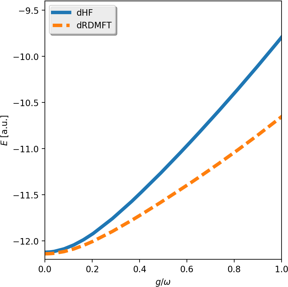
Figure 7: The plot shows the total energy of the dressed HF and dressed RDMFT calculations of $Be$ for increasing $g/\omega$. We observe the same trend as for the two-electron systems: for both levels of theory, the energy grows with increasing $g/\omega$, though for dressed HF faster than for dressed RDMFT.

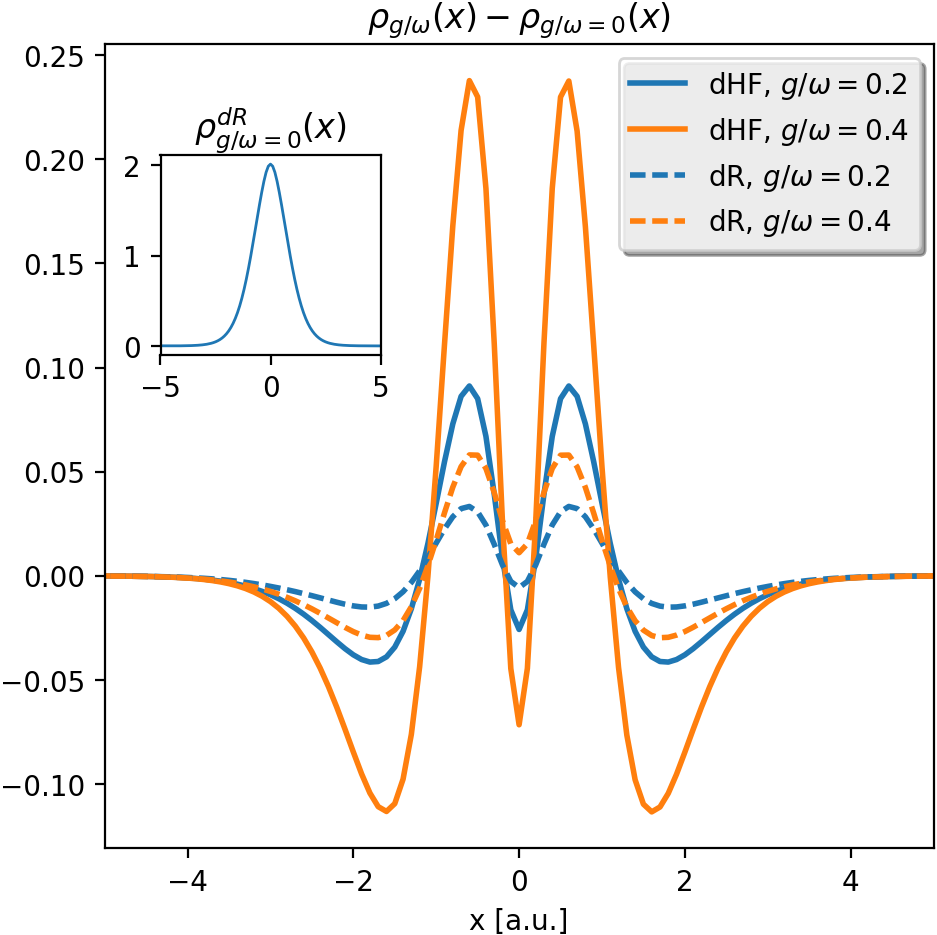
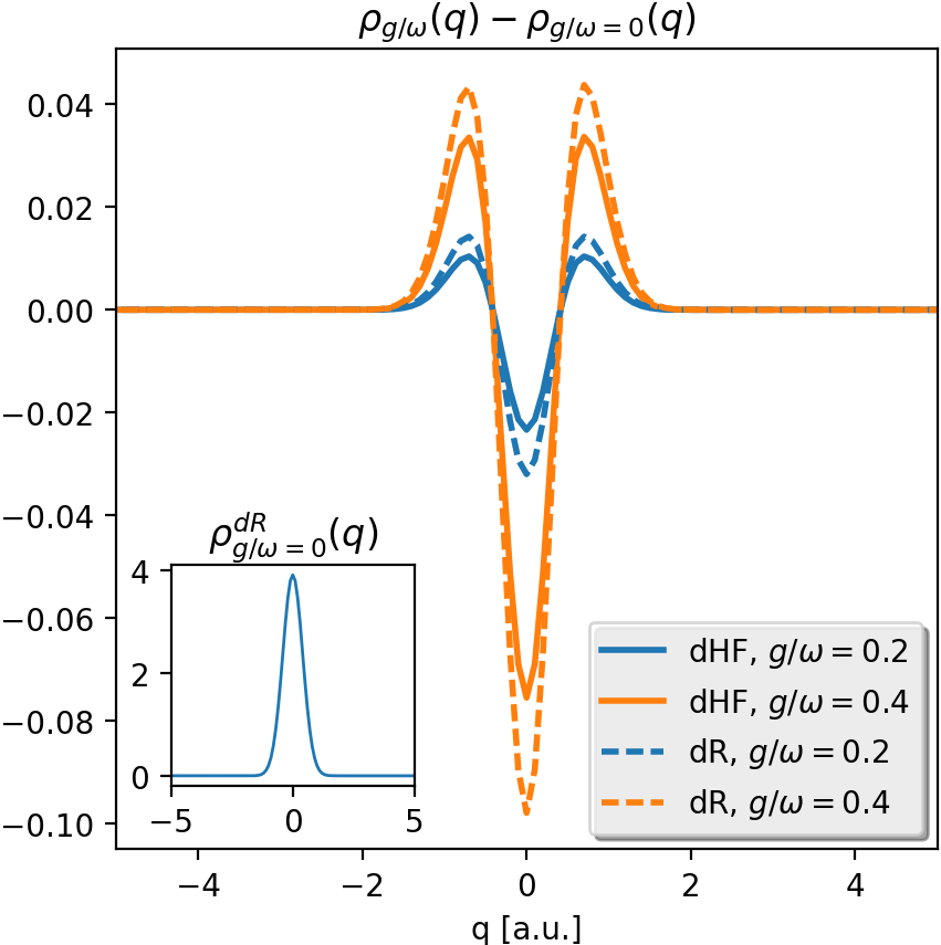
Figure 8: Shown are the electronic ($\rho^{dHF/dR}_{g/\omega}(x)$, left) and photonic ($\rho^{dHF/dR}_{g/\omega}(q)$, right) densities of $Be$ for dressed HF (dHF) and dressed RDMFT (dR) for 2 different coupling strengths subtracted from their counterparts in the no-coupling limit ($\rho^{dHF/dR}_{g/\omega=0}(x/q)$.) We see in the electronic (photonic) case that the dressed RDMFT deviations are less (more) pronounced than for dressed HF.

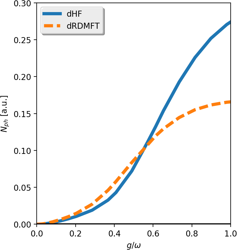
Figure 9: The total mode occupation $N_{ph}$ for dressed HF and dressed RDMFT is shown for $Be$. We see that dressed RDMFT exhibits larger $N_{ph}$ until a coupling strength of $g/\omega\approx 0.5$. For larger coupling the dressed HF mode occupation becomes higher.

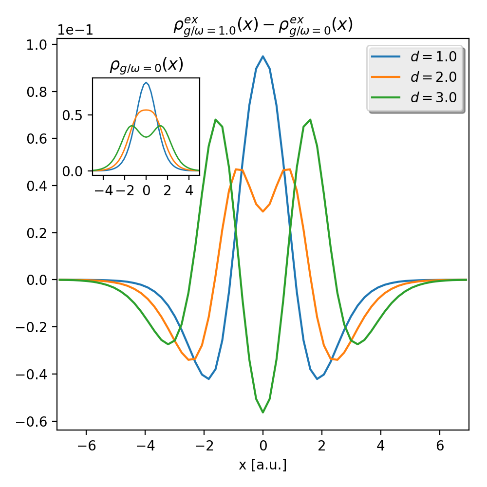
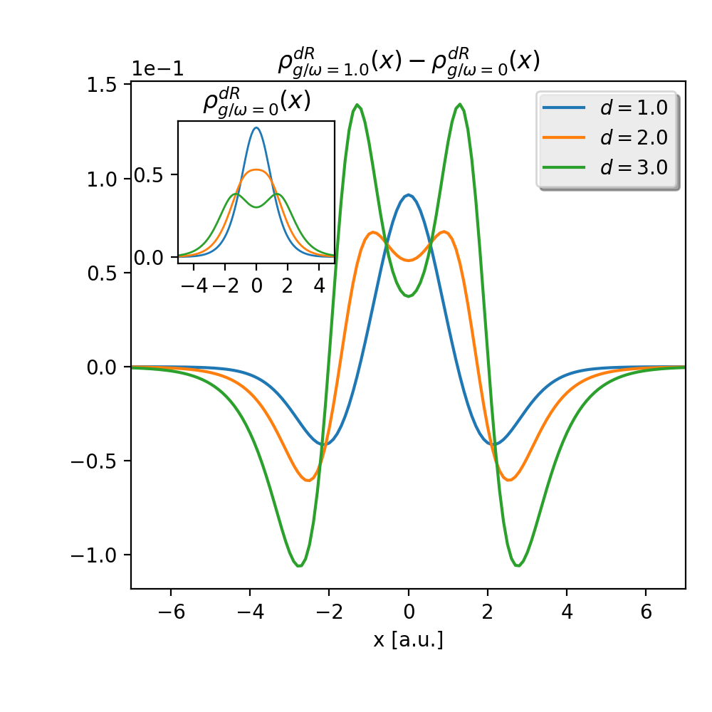
Figure 10: We show the differences in the electronic density of the $H_{2}$ molecule for 3 different bond lengths $d$ (as examples of the dissociation) for $g/\omega=1.0$ compared to $g/\omega=0$, calculated exactly ($\rho^{ex}_{g/\omega}(x)$, left) and with dressed RDMFT ($\rho^{dR}_{g/\omega}(x)$, right). We see that for small $d$, the cavity mode reduces the electronic repulsion and localizes the charges at the bond center ($d=1<d_{eq}=1.628$) in comparison to the free molecule (insets.) For larger $d$, the electronic repulsion is locally enhanced such that the charge deviations are separated in two peaks ($d=2$.) For very large $d$, this interplay between local suppresion and enhancement of repulsion becomes more pronounced ($d=3$.) The dressed RDMFT calculations capture the behavior very well.

We conclude this section with two examples, for which the light-matter interaction changes the bare systems non-trivially, depending not only on the coupling strength but also on the details of the electronic structure. We start with the dissociation of $H_{2}$ as an example for a chemical reaction, where we use $v_{H_{2}}(x)$ with different $d$. In Fig. 10, we see the density of two H-atoms under variation of the distance $d$ with and without the (strong) coupling to the cavity. We see that the influence of the cavity mode strongly depends on the exact electronic structure. The interaction with the cavity mode can locally reduce or enhance the electronic repulsion due to the Coulomb interaction, where the exact interplay between both effects depends on the interatomic distance. Thus, we can observe a number of different effects like pure localization of the density towards the center of charge ($d=1$) or localization combined with a local enhancement of repulsion such that the density deviations exhibit a double peak structure ($d=2$.) The local enhancement of electronic repulsion can grow so strong that the density at the center of charge is reduced but at the same time the density maxima shift closer to each other, which is an effective suppression of electronic repulsion ($d=3$.) This interplay is reflected in the natural orbitals and occupation numbers. The coupling shifts a considerable amount of occupation from the first natural orbital to the second and third one. The contribution to the total density of the former (latter) has the character of enhanced (suppressed) electron repulsion. To show the potential of these effects, we present calculations in the deep-strong coupling regime with $g/\omega=1.0$, where the effects reach the order of 10 % of the unperturbed density, which is enormous. For smaller coupling strengths of the order of $g/\omega=0.1$, these effects are as diverse, but naturally smaller with density deformations of the order of $10^{-3}$. However, as every observable depends on the density, such deviations are significant. Remarkably, dressed RDMFT reproduces the effects accurately.

\begin{overpic}[width=212.47617pt]{He_dR_dens_lam_diff_x} \put(85.0,20.0){{\color[rgb]{0,0,0}He}}\hfill\end{overpic}

\begin{overpic}[width=212.47617pt]{Be_dR_dens_lam_diff_x} \put(85.0,20.0){{\color[rgb]{0,0,0}Be}}\hfill\end{overpic}

Figure 11: We show the differences in the electronic density ($\rho_{g/\omega}(x)$) of $He$ (left) and $Be$ (right) for 3 different coupling strengths compared to the atoms outside the cavity (insets,) calculated with dressed RDMFT. We see that the effect of the cavity is very different for both systems: The strong localization of the electronic density for $He$ indicates the suppression of electronic repulsion for all coupling strengths. For $Be$ instead, we see additionally local enhancement of the repulsion. The interplay of enhancement and suppression changes with increasing coupling strength.

In the second example, we compare the behavior of the $He$ and $Be$ atoms under the influence of the cavity. Though the shapes of the electronic density of the two bare systems are very similar (see insets in Fig. 11,) they behave very differently under the influence of the cavity, which can be seen in Fig. 11. The electronic density of $He$ is pushed towards its center of charge with increasing coupling strength, which can be understood as a suppression of the electronic repulsion induced by the Coulomb interaction. As $He$ can be understood very well with only one orbital this is to be expected. Things change for $Be$, where we have several dominant orbitals. With increasing coupling strength, we see like in the dissociation example a subtle interplay between suppression and local enhancement of the electronic repulsion, that depends on the coupling strength. Thus for the same coupling strength, we can observe opposite ($g/\omega=0.1$ and $0.4$ in the plot) but also similar effects ($g/\omega=0.8$ in the plot) in two systems that have almost the same “bare” density shape. Like in the dissociation example, this intricate behavior can be understood by the interplay of the different natural orbitals contributing to the electronic density. In this particular case, the main physics happens in the second and third natural orbital, where the former (with a double-peak structure) loses a considerable amount of occupation to the latter (with a triple peak structure) with increasing coupling strength.

These (seemingly simple) examples show how subtle details of the electronic structure influence the changes induced by the coupling to photons. We see a non-trivial interplay between local suppression and enhancement of the Coulomb induced repulsion between the particles. This is reflected in the natural orbitals and occupation numbers of the light-matter system and thus influences all possible observables. Such small changes have been shown to theoretically affect chemical properties and reactions strongly, which are determined by an intricate interplay between Coulomb and photon induced correlations ²⁸. Whether these modifications of the underlying electronic structure are indeed a major player in the changes of chemical and physical properties still needs to be seen. However, to capture such modifications in the first place (and study their influence) clearly needs an ab-initio theory that is able to treat both types of (strong) correlations accurately and is predictive inside as well as outside of a cavity. We have shown here that dressed RDMFT is a viable option to predict and analyze these intricate structural changes.

Conclusion

In this work we presented a RDMFT formalism for coupled matter-photon systems. This formalism is capable to account for the full quantum-mechanical degrees of freedom of the coupled fermion-boson problem. We discussed that extending the standard formulation of electronic RDMFT to systems with coupled fermionic and bosonic degrees of freedom is not straightforward. Then, we presented an alternative approach which overcomes most of the intricate representability issues by embedding the coupled matter-photon system in a higher-dimensional auxiliary space. Specifically, we introduced for a problem with $N$ electrons coupled to $M$ photon modes, $(N-1)M$ auxiliary coordinates, which allowed us to “fermionize” the coupled problem with respect to new polaritonic coordinates. The resulting dressed fermionic particles are governed by a Hamiltonian with only 1-body and 2-body terms and thus, one can apply any standard electronic-structure method. The extension is constructed in such a way that the auxiliary dimensions do not modify the original physical system and the physical observables are easy to recover. Notably, besides the possibility to study modifications of electronic systems due to a cavity mode, dressed RDMFT offers also the possibility to calculate purely photonic observables like the mode occupation or fluctuations of the electric and magnetic field. We used this framework to develop and implement dressed RDMFT in the electronic-structure code Octopus ⁸⁸, and tested it with the Hartree-Fock and Müller functional. For simple one-dimensional models of atoms and molecules the obtained approximate results were in good agreement with the exact results from the weak to the deep-strong coupling regime. We then used our method to show that the modifications due to strong matter-photon coupling are far from trivial and depend on the detailed electronic structure. For a molecular as well as an atomic system we showed that strong coupling can locally enhance and suppress the Coulomb induced repulsion between electrons. This behaviour does not only depend on the strength of the matter-photon coupling but also on the details of the matter subsystem (e.g. the interatomic distance of the atoms of a molecule.) We showed that our method allows to predict the structures accurately inside and outside of the cavity and furthermore extends the well-established tools of natural orbitals to analyze coupled light-matter systems.

Although the presented method is practical only for a few photon modes, since the number of photon modes determines the dimension of the involved dressed orbitals, it is exactly these cases that are the most relevant in cavity and circuit QED experiments. Since dressed RDMFT is non-perturbative and seems to be accurate over a wide range of couplings, it is a promising tool to investigate long-standing problems of quantum optics, such as the quest for a super-radiant phase in the ground state of strongly-coupled matter-photon systems ²⁴. Moreover, it is a very promising tool to investigate changes in the ground-state due to matter-photon coupling that can possibly modify chemical reactions ⁵. Recently, it has been shown that charge-transfer processes can be considerably modified due to strong coupling to a cavity mode²⁸. And although the presented results were for reduced dimensionality, an extension to three spatial dimensions is straightforward. We can rely here again on an already existing implementation for RDMFT in Octopus. Work along these lines is in progress. Besides such interesting applications and fundamental questions of light matter-interactions, there are many open questions to answer also in the presented theory itself. For instance, how strong is the influence of the hitherto negelected $q$-exchange symmetry? First calculations for many particles indicate that it will become important to enforce this extra symmetry to stay accurate when going from the weak to the deep-strong coupling regime. Furthermore, it might become beneficial to avoid the “fermionization” that we employed and then very interesting mathematical questions about $N$-representability for coupled fermion-boson systems need to be addressed. Here, the understanding how to enforce the $q$-exchange symmetries in the dressed formulation could be very useful.

F.B. would like to thank Nicole Helbig, Klaas Giesbertz, Micael Oliveira, and Christian Schäfer for stimulating and useful discussions. We acknowledge financial support from the European Research Council (ERC-2015-AdG-694097).

Survey on the bosonic symmetry of the photon wave function. Details about the convergence study of the numerical examples shown in the paper. Protocol for the convergence of a dressed HF/RDMFT calculation.

References

- Ebbesen 2016 Ebbesen, T. W. Hybrid Light–Matter States in a Molecular and Material Science Perspective. Accounts of Chemical Research 2016, 49, 2403–2412
- Sukharev and Nitzan 2017 Sukharev, M.; Nitzan, A. Optics of exciton-plasmon nanomaterials. Journal of Physics: Condensed Matter 2017, 29, 443003
- Kockum et al. 2018 Kockum, A. F.; Miranowicz, A.; De Liberato, S.; Savasta, S.; Nori, F. Ultrastrong coupling between light and matter. Nat. Rev. Phys. 2018, 1, 19–40
- Hutchison et al. 2012 Hutchison, J. A.; Schwartz, T.; Genet, C.; Devaux, E.; Ebbesen, T. W. Modifying chemical landscapes by coupling to vacuum fields. Angew. Chemie - Int. Ed. 2012, 51, 1592–1596
- Thomas et al. 2016 Thomas, A.; George, J.; Shalabney, A.; Dryzhakov, M.; Varma, S. J.; Moran, J.; Chervy, T.; Zhong, X.; Devaux, E.; Genet, C. Ground-State Chemical Reactivity under Vibrational Coupling to the Vacuum Electromagnetic Field. Angewandte Chemie 2016, 128, 11634–11638
- Firstenberg et al. 2013 Firstenberg, O.; Peyronel, T.; Liang, Q. Y.; Gorshkov, A. V.; Lukin, M. D.; Vuletić, V. Attractive photons in a quantum nonlinear medium. Nature 2013, 502, 71–75
- Goban et al. 2015 Goban, A.; Hung, C. L.; Hood, J. D.; Yu, S. P.; Muniz, J. A.; Painter, O.; Kimble, H. J. Superradiance for Atoms Trapped along a Photonic Crystal Waveguide. Phys. Rev. Lett. 2015, 115, 063601
- Coles et al. 2014 Coles, D. M.; Yang, Y.; Wang, Y.; Grant, R. T.; Taylor, R. A.; Saikin, S. K.; Aspuru-Guzik, A.; Lidzey, D. G.; Tang, J. K.-H.; Smith, J. M. Strong coupling between chlorosomes of photosynthetic bacteria and a confined optical cavity mode. Nature communications 2014, 5, 5561
- Orgiu et al. 2015 Orgiu, E.; George, J.; Hutchison, J. A.; Devaux, E.; Dayen, J. F.; Doudin, B.; Stellacci, F.; Genet, C.; Schachenmayer, J.; Genes, C.; Pupillo, G.; Samorì, P.; Ebbesen, T. W. Conductivity in organic semiconductors hybridized with the vacuum field. Nat. Mater. 2015, 14, 1123–1129
- Andrew and Barnes 2004 Andrew, P.; Barnes, W. L. Energy transfer across a metal film mediated by surface plasmon polaritons. Science 2004, 306, 1002–1005
- Dicke 1954 Dicke, R. H. Coherence in spontaneous radiation processes. Phys. Rev. 1954, 93, 99–110
- Todorov et al. 2010 Todorov, Y.; Andrews, A. M.; Colombelli, R.; De Liberato, S.; Ciuti, C.; Klang, P.; Strasser, G.; Sirtori, C. Ultrastrong light-matter coupling regime with polariton dots. Phys. Rev. Lett. 2010, 105, 1–4
- Michetti et al. 2015 Michetti, P.; Mazza, L.; La Rocca, G. C. In Organic Nanophotonics: Fundamentals and Applications; Zhao, Y. S., Ed.; Springer Berlin Heidelberg: Berlin, Heidelberg, 2015; pp 39–68
- Cwik et al. 2016 Cwik, J. A.; Kirton, P.; De Liberato, S.; Keeling, J. Excitonic spectral features in strongly coupled organic polaritons. Phys. Rev. A 2016, 93, 1–12
- Galego et al. 2016 Galego, J.; Garcia-Vidal, F. J.; Feist, J. Suppressing photochemical reactions with quantized light fields. Nat. Commun. 2016, 7, 1–6
- Feist et al. 2018 Feist, J.; Galego, J.; Garcia-Vidal, F. J. Polaritonic Chemistry with Organic Molecules. ACS Photonics 2018, 5, 205–216
- Feist and Garcia-Vidal 2015 Feist, J.; Garcia-Vidal, F. J. Extraordinary exciton conductance induced by strong coupling. Phys. Rev. Lett. 2015, 114, 1–5
- Herrera and Spano 2016 Herrera, F.; Spano, F. C. Cavity-Controlled Chemistry in Molecular Ensembles. Phys. Rev. Lett. 2016, 116, 1–6
- Cirio et al. 2016 Cirio, M.; De Liberato, S.; Lambert, N.; Nori, F. Ground State Electroluminescence. Phys. Rev. Lett. 2016, 116, 1–7
- Kockum et al. 2017 Kockum, A. F.; MacRì, V.; Garziano, L.; Savasta, S.; Nori, F. Frequency conversion in ultrastrong cavity QED. Sci. Rep. 2017, 7, 1–13
- De Liberato 2014 De Liberato, S. Light-matter decoupling in the deep strong coupling regime: The breakdown of the purcell effect. Phys. Rev. Lett. 2014, 112, 1–5
- De Liberato 2017 De Liberato, S. Virtual photons in the ground state of a dissipative system. Nat. Commun. 2017, 8, 1–6
- Gely et al. 2017 Gely, M. F.; Parra-Rodriguez, A.; Bothner, D.; Blanter, Y. M.; Bosman, S. J.; Solano, E.; Steele, G. A. Convergence of the multimode quantum Rabi model of circuit quantum electrodynamics. Phys. Rev. B 2017, 95, 1–5
- De Bernardis et al. 2018 De Bernardis, D.; Pilar, P.; Jaako, T.; De Liberato, S.; Rabl, P. Breakdown of gauge invariance in ultrastrong-coupling cavity QED. Phys. Rev. A 2018, 98, 1–16
- Sánchez Muñoz et al. 2018 Sánchez Muñoz, C.; Nori, F.; De Liberato, S. Resolution of superluminal signalling in non-perturbative cavity quantum electrodynamics. Nat. Commun. 2018, 9, 1924
- Jaako et al. 2016 Jaako, T.; Xiang, Z. L.; Garcia-Ripoll, J. J.; Rabl, P. Ultrastrong-coupling phenomena beyond the Dicke model. Phys. Rev. A 2016, 94, 1–10
- Schäfer et al. 2018 Schäfer, C.; Ruggenthaler, M.; Rubio, A. Ab initio nonrelativistic quantum electrodynamics: Bridging quantum chemistry and quantum optics from weak to strong coupling. Physical Review A 2018, 98, 043801
- Schäfer et al. 2019 Schäfer, C.; Ruggenthaler, M.; Appel, H.; Rubio, A. Modification of excitation and charge transfer in cavity quantum-electrodynamical chemistry. Proc. Natl. Acad. Sci. 2019, 116, 4883–4892
- Galego et al. 2015 Galego, J.; Garcia-Vidal, F. J.; Feist, J. Cavity-induced modifications of molecular structure in the strong-coupling regime. Phys. Rev. X 2015, 5, 1–14
- Kowalewski et al. 2016 Kowalewski, M.; Bennett, K.; Mukamel, S. Non-adiabatic dynamics of molecules in optical cavities. The Journal of chemical physics 2016, 144, 054309
- Garcia-Vidal and Feist 2017 Garcia-Vidal, F. J.; Feist, J. Long-distance operator for energy transfer. Science 2017, 357, 1357–1358
- Zeb et al. 2017 Zeb, M. A.; Kirton, P. G.; Keeling, J. Exact states and spectra of vibrationally dressed polaritons. ACS Photonics 2017, 5, 249–257
- Luk et al. 2017 Luk, H. L.; Feist, J.; Toppari, J. J.; Groenhof, G. Multiscale molecular dynamics simulations of polaritonic chemistry. Journal of chemical theory and computation 2017, 13, 4324–4335
- del Pino et al. 2018 del Pino, J.; Schröder, F. A.; Chin, A. W.; Feist, J.; Garcia-Vidal, F. J. Tensor network simulation of polaron-polaritons in organic microcavities. Physical Review B 2018, 98, 165416
- Ruggenthaler et al. 2018 Ruggenthaler, M.; Tancogne-Dejean, N.; Flick, J.; Appel, H.; Rubio, A. From a quantum-electrodynamical light–matter description to novel spectroscopies. Nat. Rev. Chem. 2018, 2, 0118
- Groenhof and Toppari 2018 Groenhof, G.; Toppari, J. J. Coherent light harvesting through strong coupling to confined light. The journal of physical chemistry letters 2018, 9, 4848–4851
- Vendrell 2018 Vendrell, O. Collective Jahn-Teller interactions through light-matter coupling in a cavity. Physical review letters 2018, 121, 253001
- Reitz et al. 2019 Reitz, M.; Sommer, C.; Genes, C. Langevin approach to quantum optics with molecules. Physical review letters 2019, 122, 203602
- Triana and Sanz-Vicario 2019 Triana, J. F.; Sanz-Vicario, J. L. Revealing the Presence of Potential Crossings in Diatomics Induced by Quantum Cavity Radiation. Physical review letters 2019, 122, 063603
- Galego et al. 2019 Galego, J.; Climent, C.; Garcia-Vidal, F. J.; Feist, J. Cavity Casimir-Polder forces and their effects in ground state chemical reactivity. Phys. Rev. X 2019, 9, 1–22
- Csehi et al. 2019 Csehi, A.; Kowalewski, M.; Halász, G. J.; Vibók, Á. Ultrafast dynamics in the vicinity of quantum light-induced conical intersections. arXiv preprint arXiv:1902.03640 2019,
- Martínez-Martínez et al. 2018 Martínez-Martínez, L. A.; Ribeiro, R. F.; Campos-González-Angulo, J.; Yuen-Zhou, J. Can Ultrastrong Coupling Change Ground-State Chemical Reactions? ACS Photonics 2018, 5, 167–176
- Viehmann et al. 2011 Viehmann, O.; Von Delft, J.; Marquardt, F. Superradiant phase transitions and the standard description of circuit QED. Phys. Rev. Lett. 2011, 107, 1–5
- R. Dreizler 1990 R. Dreizler, E. G. Density Functional Theory- An Approach to the Quantum Many-Body Problem; Springer Berlin Heidelberg, 1990
- Dreizler and Engel 2011 Dreizler, R. M.; Engel, E. Density Functional Theory: An Advanced Course; Springer, 2011
- Fetter and Walecka 2003 Fetter, A.; Walecka, J. Quantum Theory of Many-Particle Systems; Dover, Mineola, New York, 2003
- Stefanucci and Van Leeuwen 2013 Stefanucci, G.; Van Leeuwen, R. Nonequilibrium many-body theory of quantum systems: a modern introduction; Cambridge University Press, 2013
- Onida et al. 2002 Onida, G.; Reining, L.; Rubio, A. Electronic excitations: Density-functional versus many-body Green’s-function approaches. Rev. Mod. Phys. 2002, 74, 601–659
- Theophilou et al. 2018 Theophilou, I.; Buchholz, F.; Eich, F. G.; Ruggenthaler, M.; Rubio, A. Kinetic-Energy Density-Functional Theory on a Lattice. J. Chem. Theory Comput. 2018, 14, 4072–4087
- Ruggenthaler et al. 2011 Ruggenthaler, M.; Mackenroth, F.; Bauer, D. Time-dependent Kohn-Sham approach to quantum electrodynamics. Physical Review A 2011, 84, 042107
- Tokatly 2013 Tokatly, I. V. Time-dependent density functional theory for many-electron systems interacting with cavity photons. Phys. Rev. Lett. 2013, 110, 1–5
- Ruggenthaler et al. 2014 Ruggenthaler, M.; Flick, J.; Pellegrini, C.; Appel, H.; Tokatly, I. V.; Rubio, A. Quantum-electrodynamical density-functional theory: Bridging quantum optics and electronic-structure theory. Phys. Rev. A 2014, 90, 1–26
- Ruggenthaler 2015 Ruggenthaler, M. Ground-State Quantum-Electrodynamical Density-Functional Theory. arXiv Preprint 2015, arXiv:1509, 1–6
- Flick et al. 2015 Flick, J.; Ruggenthaler, M.; Appel, H.; Rubio, A. Kohn–Sham approach to quantum electrodynamical density-functional theory: Exact time-dependent effective potentials in real space. Proc. Natl. Acad. Sci. 2015, 112, 15285–15290
- Flick et al. 2017 Flick, J.; Ruggenthaler, M.; Appel, H.; Rubio, A. Atoms and molecules in cavities, from weak to strong coupling in quantum-electrodynamics (QED) chemistry. Proc. Natl. Acad. Sci. 2017, 114, 3026–3034
- Flick et al. 2018 Flick, J.; Schäfer, C.; Ruggenthaler, M.; Appel, H.; Rubio, A. Ab Initio Optimized Effective Potentials for Real Molecules in Optical Cavities: Photon Contributions to the Molecular Ground State. ACS Photonics 2018, 5, 992–1005
- Flick et al. 2018 Flick, J.; Welakuh, D. M.; Ruggenthaler, M.; Appel, H.; Rubio, A. Light-Matter Response Functions in Quantum-Electrodynamical Density-Functional Theory: Modifications of Spectra and of the Maxwell Equations. arXiv Preprint arXiv:1803.02519 2018, 1–27
- Cohen et al. 2012 Cohen, A. J.; Mori-Sánchez, P.; Yang, W. Challenges for Density Functional Theory. Chemical Reviews 2012, 112, 289–320
- Niemczyk et al. 2010 Niemczyk, T.; Deppe, F.; Huebl, H.; Menzel, E. P.; Hocke, F.; Schwarz, M. J.; Zueco, D.; Hümmer, T.; Solano, E.; Marx, A.; Gross, R. Circuit quantum electrodynamics in the ultrastrong-coupling regime. Nat. Phys. 2010, 6, 772–776
- Bayer et al. 2017 Bayer, A.; Pozimski, M.; Schambeck, S.; Schuh, D.; Huber, R.; Bougeard, D.; Lange, C. Terahertz Light-Matter Interaction beyond Unity Coupling Strength. Nano Lett. 2017, 17, 6340–6344
- Gilbert 1975 Gilbert, T. L. Hohenberg-Kohn theorem for nonlocal external potentials. Phys. Rev. B 1975, 12, 2111–2120
- Müller 1984 Müller, A. M. K. Explicit approximate relation between reduced two- and one-particel density matrices. Phys. Lett. 1984, 105, 446
- Goedecker and Umrigar 1998 Goedecker, S.; Umrigar, C. J. Natural orbital functional for the many-electron problem. Phys. Rev. Lett. 1998, 81, 866–869
- Sharma et al. 2013 Sharma, S.; Dewhurst, J. K.; Shallcross, S.; Gross, E. K. U. Spectral density and metal-insulator phase transition in mott insulators within reduced density matrix functional theory. Phys. Rev. Lett. 2013, 110, 1–5
- Coleman 1963 Coleman, A. J. Structure of Fermion Density Matrices. Rev. Mod. Phys. 1963, 35, 668–686
- Klyachko 2006 Klyachko, A. A. Quantum marginal problem and N-representability. Journal of Physics: Conference Series 2006, 36, 72
- Mazziotti 2012 Mazziotti, D. A. Structure of Fermionic Density Matrices: Complete -Representability Conditions. Phys. Rev. Lett. 2012, 108, 263002
- Nielsen et al. 2018 Nielsen, S. E. B.; Schäfer, C.; Ruggenthaler, M.; Rubio, A. Dressed-Orbital Approach to Cavity Quantum Electrodynamics and Beyond. arXiv preprint arXiv:1812.00388 2018,
- Grynberg et al. 2010 Grynberg, G.; Aspect, A.; Fabre, C. Introduction to quantum optics: from the semi-classical approach to quantized light; Cambridge University Press, 2010
- Rokaj et al. 2018 Rokaj, V.; Welakuh, D. M.; Ruggenthaler, M.; Rubio, A. Light–matter interaction in the long-wavelength limit: no ground-state without dipole self-energy. Journal of Physics B: Atomic, Molecular and Optical Physics 2018, 51, 034005
- Spohn 2004 Spohn, H. Dynamics of charged particles and their radiation field; Cambridge university press, 2004
- Power and Thirunamachandran 1982 Power, E. A.; Thirunamachandran, T. Quantum electrodynamics in a cavity. Phys. Rev. A 1982, 25, 2473–2484
- Shahbazyan and Stockman 2013 Shahbazyan, T. V.; Stockman, M. I. Plasmonics: theory and applications; Springer, 2013
- Giesbertz and Ruggenthaler 2019 Giesbertz, K. J. H.; Ruggenthaler, M. One-body reduced density-matrix functional theory in finite basis sets at elevated temperatures. Phys. Rep. 2019, 806, 1–47
- Bonitz 2016 Bonitz, M. Quantum Kinetic Theory, 2nd ed.; Springer: Berlin, 2016
- van Leeuwen and Stefanucci 2013 van Leeuwen, R.; Stefanucci, G. Nonequilibrium Many-Body Theory of Quantum Systems; Cambridge University Press, 2013
- Coleman and Yukalov 2000 Coleman, A. J.; Yukalov, V. I. Reduced density matrices: Coulson’s challenge; Springer Science & Business Media, 2000; Vol. 72
- Coulson 1960 Coulson, C. Present State of Molecular Structure Calculations. Rev. Mod. Phys. 1960, 32, 170–177
- Rokaj et al. 2019 Rokaj, V.; Penz, M.; Sentef, M. A.; Ruggenthaler, M.; Rubio, A. Quantum Electrodynamical Bloch Theory with Homogeneous Magnetic Fields. arXiv Prepr. 2019, 1–6
- Watson 1968 Watson, J. K. Simplification of the molecular vibration-rotation Hamiltonian. Molecular Physics 1968, 15, 479–490
- Piris 2017 Piris, M. Global Method for Electron Correlation. Phys. Rev. Lett. 2017, 119, 1–5
- Mazziotti 2012 Mazziotti, D. A. Two-electron reduced density matrix as the basic variable in many-electron quantum chemistry and physics. Chem. Rev. 2012, 112, 244–262
- Hohenberg and Kohn 1964 Hohenberg, P.; Kohn, W. Inhomogeneous electron gas. Physical review 1964, 136, B864
- Theophilou et al. 2015 Theophilou, I.; Lathiotakis, N. N.; Marques, M. A.; Helbig, N. Generalized Pauli constraints in reduced density matrix functional theory. The Journal of chemical physics 2015, 142, 154108
- Lieb 1981 Lieb, E. H. Variational principle for many-fermion systems. Physical Review Letters 1981, 46, 457
- Buijse and Baerends 2002 Buijse, M. A.; Baerends, E. J. An approximate exchange-correlation hole density as a functional of the natural orbitals. Mol. Phys. 2002, 100, 401–421
- Frank et al. 2007 Frank, R. L.; Lieb, E. H.; Seiringer, R.; Siedentop, H. Müller’s exchange-correlation energy in density-matrix-functional theory. Phys. Rev. A 2007, 76, 1–16
- Andrade et al. 2015 Andrade, X. et al. Real-space grids and the Octopus code as tools for the development of new simulation approaches for electronic systems. Phys. Chem. Chem. Phys. 2015, 17, 31371–31396
- J. M. Ugalde 2008 J. M. Ugalde, M. P. Iterative Diagonalization for Orbital Optimization in Natural Orbital Functional Theory. J. Comput. Chem. 2008, 30, 1545–1614
- Ruggenthaler and Bauer 2009 Ruggenthaler, M.; Bauer, D. Rabi oscillations and few-level approximations in time-dependent density functional theory. Phys. Rev. Lett. 2009, 102, 2–5
- Fuks et al. 2011 Fuks, J. I.; Helbig, N.; Tokatly, I. V.; Rubio, A. Nonlinear phenomena in time-dependent density-functional theory: What Rabi oscillations can teach us. Phys. Rev. B 2011, 84