Search for invisible modes of nucleon decay in water with the SNO+ detector

Abstract

This paper reports results from a search for nucleon decay through ‘invisible’ modes, where no visible energy is directly deposited during the decay itself, during the initial water phase of SNO+. However, such decays within the oxygen nucleus would produce an excited daughter that would subsequently de-excite, often emitting detectable gamma rays. A search for such gamma rays yields limits of 2.5$\times 10^{29}$ y at 90% Bayesian credibility level (with a prior uniform in rate) for the partial lifetime of the neutron, and 3.6$\times 10^{29}$ y for the partial lifetime of the proton, the latter a 70% improvement on the previous limit from SNO. We also present partial lifetime limits for invisible dinucleon modes of 1.3$\times 10^{28}$ y for $nn$, 2.6$\times 10^{28}$ y for $pn$ and 4.7$\times 10^{28}$ y for $pp$, an improvement over existing limits by close to three orders of magnitude for the latter two.

I Introduction

Violation of baryon number conservation is predicted by many Grand Unified Theories Georgi and Glashow (1974) potentially explaining the matter-antimatter asymmetry of the universe. Searches for the decay of protons or bound neutrons act as important constraints on our understanding of physics beyond the Standard Model.

Modes of nucleon decay involving visible energy deposition by decay products, such as positrons, pions or kaons, have so far not been observed by large scale detectors Abe et al. (2017a, b, ). As such, interest has turned to less well-constrained decay modes that could have escaped detection. A potential set of channels are the invisible decay modes in which one or more nucleon decays to final states which go undetected, such as those with neutrinos, other exotic neutral, weakly-interacting particles or charged particles with velocities below the Cherenkov threshold. Although no prompt signal would be observed from the particles directly emitted in the decay, the remaining nucleus would be left in an excited state, and could then emit a detectable signal as it de-excites. The search for the de-excitation signal of the final state nucleus is model-independent, as it puts no requirements on the particles produced in the decay. Theoretical models include modes with decays to three neutrinos Mohapatra and Perez-Lorenzana (2003) or to non-Standard Model particles such as the unparticle He and Pakvasa (2008) or dark fermions D. Barducci and Gabrielli (2018), the latter providing a possible solution to the neutron lifetime puzzle Fornal and Grinstein (2018).

The Sudbury Neutrino Observatory (SNO) and KamLAND experiments have conducted searches for such model-independent modes with KamLAND setting the current best limit for the invisible neutron decay lifetime of $\tau(n\rightarrow\mathrm{inv.})$ > $5.8\times 10^{29}$ y at 90% C.L. Araki et al. (2006) and SNO setting the best limit for invisible proton decays of $2.1\times 10^{29}$ y Ahmed et al. (2004), improving on previous limits by the Borexino Counting Test Facility (CTF) Back et al. (2003) and Kamiokande Suzuki et al. (1993). Limits also exist for the dinucleon modes of 1.4$\times 10^{30}$ y Araki et al. (2006) for the $nn$ mode from KamLAND, 5.0$\times 10^{25}$ y Back et al. (2003) for the $pp$ mode by the Borexino CTF and 2.1$\times 10^{25}$ y Tretyak et al. (2004) for the $pn$ mode.

The SNO+ experiment has been running since December 2016, taking commissioning data with the detector filled with ultrapure water. During this phase, a new search has been made for invisible nucleon decay via the decay of ¹⁶O. After an invisible nucleon decay, the ¹⁶O is left in either the ¹⁵O* excited state, if the decaying nucleon was a neutron, or in the ¹⁵N* state, if the decaying nucleon was a proton. 44% of the time, ¹⁵O* will de-excite to produce a 6.18 MeV gamma, and 2% of the time, the decay will produce a 7.03 MeV gamma. Similarly, ¹⁵N* will produce a 6.32 MeV gamma in 41% of decays, with 7.01, 7.03 and 9.93 MeV gammas produced 2, 2 and 3% of the time, respectively Ejiri (1993).

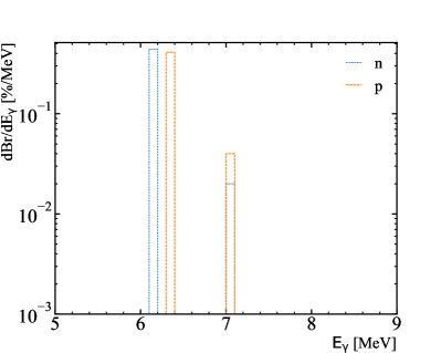
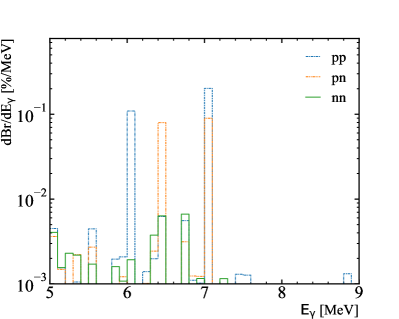
Figure 1: Spectrum of de-excitation gamma rays emitted after the invisible decay of ¹⁶O for single nucleon decay Ejiri (1993) (left) and dinucleon decay Hagino and Nirkko (2018) (right) as a function of gamma ray energy $E_{\gamma}$ between 5 and 9 MeV.

This search has a unique sensitivity for two reasons: firstly, the branching fraction to produce a visible signal of a de-exciting oxygen nucleus is larger than the 5.8% for carbon Kamyshkov and Kolbe (2003) used by KamLAND. Secondly, the use of H₂O rather than heavy-water (D₂O) removes the solar neutrino charged-current and neutral-current signals, major backgrounds in the SNO search.

Dinucleon modes are also sought, based on the emission of de-excitation gamma rays from ¹⁴O^∗, ¹⁴N^∗ and ¹⁴C^∗ for the $nn$, $pn$ and $pp$ invisible decay modes, respectively Hagino and Nirkko (2018). The $pp$ decay can lead to gammas of 6.09 MeV at 10.9% and 7.01 MeV at 20.1%, and the $pn$ decay has a 6.45 MeV gamma with 7.7% and 7.03 MeV gamma with 8.9% probability. The $nn$ decay proceeds via many channels, with a summed branching ratio of 4.53% for gamma emission between 5 and 9 MeV. The branching ratio for single and dinucleon decay are shown in Fig. 1.

II The SNO+ Detector

The SNO+ detector is inherited from SNO Ahmed et al. (2000), with several major upgrades to enable the use of liquid scintillator as the primary target rather than D₂O. The detector consists of a 6 m-radius spherical acrylic vessel (AV) surrounded by 9394 inward-facing photomultiplier tubes (PMTs) mounted on a stainless steel support structure with an 8 m radius from the center of the AV. During the initial water phase, the AV was filled with approximately 905 tonnes of ultrapure water. The cavity where the detector is installed is also filled with ultrapure water to shield the innermost regions from radioactivity in the PMTs and the surrounding rock. Among the upgrades for SNO+ was a new rope net to counteract the buoyancy of the scintillator and hold down the AV Bialek et al. (2016). The PMTs and front-end electronics have been reused, with work done to repair PMTs that failed over the lifetime of SNO. Aspects of the trigger system and data acquisition (DAQ) software were upgraded to handle the higher data rates and light yield expected in the scintillator phase.

III Data Selection

The results reported in this paper are based on the analysis of 235 days of data recorded between May 4th 2017 and December 25th 2017. During this time, the detector was live for 95% of the time, with 16.9% of that spent performing calibration or maintenance. A series of data quality checks were made to select the data for analysis with specific selection criteria for the detector state, event rate, occupancy, and number of poorly calibrated channels, resulting in the rejection of 29.3% of the live time. The removal of time-correlated instrumental effects, cosmic ray muon events, and trigger dead time between events resulted in the loss of an additional 2.4% of live time. The final analyzed data set has a live time of 114.7 days with an uncertainty of 0.04%.

During the SNO+ water phase, significant work was done on commissioning the water processing and recirculation systems. Changing background levels associated with these activities motivated a time-dependent analysis. The data were split into six data sets, during each of which the background levels were relatively stable, each with its own background estimate and set of analysis cuts. Table 1 details the live time of each data set.

Data set	1	2	3	4	5	6	Total
Duration (d)	5.1	14.9	30.7	29.4	11.5	23.2	114.7

Table 1: Live time within each data set, in days.

Channels that failed calibration checks were excluded from the analysis, though they still contributed to the hardware trigger. The number of offline channels varied over time but on average was around 800 channels. A stable and well-calibrated channel can still register hits caused by electronic cross-talk and PMT dark noise. Hit-cleaning algorithms, used to exclude cross-talk hits from the analysis, typically remove approximately 2% of hits in an event. The dark noise is measured and simulated on a run-by-run basis.

IV Event Reconstruction

IV.1 Vertex reconstruction

SNO+ uses a set of algorithms to reconstruct the position and direction of Cherenkov events based upon maximizing the likelihood of a distribution of PMT hit times that have been corrected for the time residuals, i.e., the time of flight relative to the assumed vertex position, and of the angle between the true direction and the line from the trial position to the PMT. These algorithms only consider hits on well-calibrated online channels, within 50 ns of the modal PMT hit time.

Three additional observables were used to classify events. The In Time Ratio (ITR) is the ratio of PMT hit time residuals within a prompt timing window of [$-2.5$ ns, 5 ns] to the total PMT hit time residuals in an event. $\beta_{14}$ is an isotropy parameterization based on the 1st and 4th Legendre polynomials of the distribution of PMT hits in the event Aharmim et al. (2010), calculated using the angle between two PMTs with respect to the reconstructed position. The projection of a particle’s reconstructed direction unit vector onto the corresponding event position unit vector ${\mathbb{u}}\cdot{\mathbb{r}}$ determines whether the particle appears inward- or outward-going relative to the center of the AV. For the physics and calibration analyses, it is required that ITR$>$0.55 and $-0.12<$$\beta_{14}$$<$0.95.

IV.2 Vertex systematic uncertainties

Systematic uncertainties in the reconstructed vertex were evaluated using a ¹⁶N calibration source Dragowsky et al. (2002), previously used in the SNO experiment, to produce tagged 6.1 MeV gammas.

A series of ¹⁶N scans were taken during the data taking period in 2017. During a scan, ¹⁶N data was collected in a series of runs at points spaced about 50 cm apart along the principal axes of the detector, typically through the center along the x, y and z axes, where the z axis points upwards through the neck of the AV. Additional scans were also taken off-axis in the xz and yz planes to evaluate asymmetries in the detector and reconstruction.

IV.2.1 Position uncertainties

To evaluate uncertainties associated with the reconstructed event vertex position and direction, the measured detector response to the ¹⁶N calibration source was compared with predictions from Monte Carlo simulation, shown in Fig. 2.

For events which were tagged by the source PMT and passed the $\beta_{14}$ and ITR cuts, the difference in the reconstructed vertex position and source position was taken in each of the x, y and z axes. The resulting one-dimensional distributions were fit with a distribution function representing the position of the first Compton electron, estimated from the Monte Carlo model, convolved with a Gaussian function and an exponential tail.

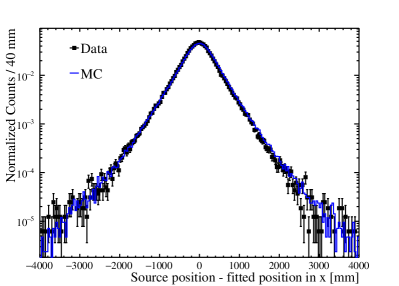
Figure 2: Comparison of the x-component of reconstructed position between ¹⁶N data acquired at a central source position and Monte Carlo simulation.

The uncertainties in reconstruction were characterized in terms of a constant offset between the position of the source and the mean reconstructed position, x$\rightarrow\mathrm{x}+\delta_{i}$, a position-dependent scale factor in which the position offset scales linearly with its value, $\mathrm{x}\rightarrow(1+\frac{\delta_{i}}{100})\mathrm{x}$, and a resolution describing the width of the distribution of reconstructed event positions, $\mathrm{x}\rightarrow\mathrm{x}+\mathcal{R}(0,\delta_{i})$, where $\mathcal{R}$ is a random number drawn from a Gaussian distribution of width $\delta_{i}$ and mean 0.

Parameter	Uncertainty, $\delta_{i}$
x offset (mm)	${}^{+16.4}_{-18.2}$
y offset (mm)	${}^{+22.3}_{-19.2}$
z offset (mm)	${}^{+38.4}_{-16.7}$
x scale (%)	${}^{+0.91}_{-1.01}$
y scale (%)	${}^{+0.92}_{-1.02}$
z scale (%)	${}^{+0.92}_{-0.99}$
x resolution (mm)	104
y resolution (mm)	98
z resolution (mm)	106
Angular resolution	${}^{+0.08}_{-0.13}$
$\beta_{14}$	$\pm 0.004$

Table 2: Systematic uncertainties in the reconstructed position and direction of events based on analysis of ¹⁶N data.

The vertex offset was calculated as the volume-weighted mean of the difference between the Gaussian fitted means of data and Monte Carlo simulation while the scale was found as the slope of a linear fit to the differences, both listed in Table 2. These were applied during signal extraction by shifting and scaling the position of each event according to the uncertainties along each axis independently and recomputing the timing probability density functions (PDFs) used for signal extraction.

The position resolution of the data events was found to be $\sim$200 mm. The difference in resolutions between the data and Monte Carlo events was modeled as a Gaussian of standard deviation $\delta_{i}=\sqrt{\sigma^{2}_{\mathrm{Data}}-\sigma^{2}_{\mathrm{MC}}}$ for each ¹⁶N run. The results were combined in a volume-weighted average, independently for each detector axis. The resulting values for $\delta_{i}$ are also listed in Table 2. These were applied during the signal extraction, smearing the positions of all Monte Carlo events by a Gaussian distribution of the appropriate width to reproduce the data.

IV.2.2 Angular resolution

Reconstructed direction is also evaluated using the ¹⁶N source, by taking into account the high degree of colinearity between Compton scattered electrons and the initial gamma direction. The angle $\theta$ between the ‘true’ direction, taken to be the vector from the source position to the reconstructed event vertex, and the reconstructed event direction was calculated and the distribution of these angles were compared for data and Monte Carlo events. To reduce the effect of position reconstruction uncertainties, only events that reconstructed more than 1200 mm from the source position were used. The resulting distributions were fit with a functional form of two exponentials as employed by SNO Aharmim et al. (2005):

$$\begin{aligned} R(\cos\theta)=~{}&\alpha_{m}\beta_{m}\frac{\mathrm{e}^{\beta_{m}(\cos\theta-1)}}{1-\mathrm{e}^{-\beta_{m}}}\\ &+(1-\alpha_{m})\beta_{s}\frac{\mathrm{e}^{\beta_{s}(\cos\theta-1)}}{1-\mathrm{e}^{-\beta_{s}}}\mathrm{,}\end{aligned}$$ (1)

where $\beta_{m}$ and $\beta_{s}$ are the slopes of the two exponential components, parameterizing the distribution for small and large angles respectively, and $\alpha_{m}$ is the fraction of the events following the exponential with slope $\beta_{m}$. The volume-weighted average of the differences in $\beta$ was computed across all runs and the resulting value used as an estimate of the uncertainty in angular resolution, transforming $\cos\theta\rightarrow 1+(\cos\theta-1)(1+\delta_{i})$. Events that were transformed beyond $-1$ were randomly assigned a value between $-1$ and 1. The resulting uncertainties are listed in Table 2.

IV.2.3 $\beta_{14}$ uncertainties

The systematic uncertainty of $\beta_{14}$, shown in Table 2, was determined from the difference between the means of Gaussian fits to data and Monte Carlo simulations of a ¹⁶N run with the source at the center of the detector. This found a shift of $-0.031\pm 0.004$, which was applied to the Monte Carlo predictions.

IV.3 Optical calibration

The detector’s optical parameters, including the attenuation and scattering of light in the water and acrylic, and the PMT angular response, are based on calibration measurements of the same materials from SNO Aharmim et al. (2010). Further optical calibrations were carried out using the ‘laserball’ Moffat. et al. (2005), a multi-wavelength laser pulse diffuser capable of running with 337, 365, 385, 420, 450 and 500 nm wavelengths, deployed within the detector.

Using the laserball data, the group velocity of light in the SNO+ water was verified to be consistent with the values used in the SNO+ simulation and reconstruction Kaye and Laby (1986).

Laserball runs were taken along the z axis after major detector maintenance periods to re-measure the PMT gain, electronic time delays and their dependence with integrated pulse charge. The delays were compared for the different laserball runs, with time drifts typically less than 0.5 ns. Larger observed drifts are consistent with actual changes in the detector hardware, for example, the replacement of offline channels.

From visual observation during detector upgrades, it is known that the reflectivity of the PMT concentrators has degraded over time. The concentrator diffuse reflectivity was tuned in simulation by comparing the PMT hit time residual spectrum between a central ¹⁶N run and its Monte Carlo simulation, with particular attention given to peaks in the late light (with residual times between 47 and 80 ns) due to reflections from the concentrators, PMT glass, and the AV. The total reflectivity was found to show no change but the diffuse reflectivity was increased from 2.0% to about 22% to provide a better match with the observed data.

The overall efficiency of the electronics and PMTs was calibrated by aligning the simulated spectrum of the number of prompt PMT hits to that from the ¹⁶N calibration data at the center of the detector.

IV.4 Energy reconstruction

The kinetic energy of an event $T_{e}$ is reconstructed by comparing the observed and expected numbers of prompt hits, defined as those with time residuals within [$-10$, 8] ns, based on simulation using the reconstructed position and direction. Since events are reconstructed under the hypothesis of an incoming electron, the observable energy of a gamma particle will reconstruct below its true energy due to the effects of Compton scattering and Cherenkov threshold, such that a 6 MeV gamma reconstructs around 5 MeV. Based upon an early ¹⁶N calibration run, 6.4 prompt PMT hits are expected per MeV of electron-equivalent deposited energy.

IV.5 Energy systematic uncertainties

The relative energy scale and detector energy resolution were determined by fitting the reconstructed energy spectrum from the ¹⁶N calibration source, as shown in Fig. 3, with the predicted energy spectrum, generated from simulation, convolved with a Gaussian distribution Dunford (2006). The fit is characterized in terms of a scale, as a linear correction to the energy, and resolution, relating to the width of the spectrum.

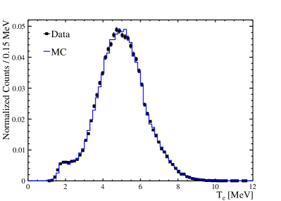
Figure 3: Comparison of reconstructed energy between ¹⁶N data acquired at a central source position and Monte Carlo simulation.

Events were associated with detector volume cells based on their reconstructed positions. The cells were distributed across z and $\rho\equiv\sqrt{\mathrm{x}^{2}+\mathrm{y}^{2}}$, with dimensions 57 cm $\times$ 200 cm, determined based on statistics. Events were also separated into seven bins based on their ${\mathbb{u}}\cdot{\mathbb{r}}$ value. In addition to 82 distinct positions from scans within the AV, the ¹⁶N source was also deployed at 19 positions along a vertical path between the AV and PMT array. Since the mean free path of the 6.1 MeV gamma is approximately 40 cm in water, all cells within the AV contained data but, due to limitations in the deployment positions of the source, some cells outside the AV were not populated. The energy scale values of the cells, mapped in z and $\rho$, were fit with a continuous function to provide a smooth calibration of energy across the detector. For each z-$\rho$ cell, fits were performed within all seven ${\mathbb{u}}\cdot{\mathbb{r}}$ bins and then averaged to provide a solid angle-weighted energy scale in the cell.

The deployment of the source was simulated at the same positions and with the same detector conditions. Half of each of the measured and simulated data sets were used to calibrate the energy scale as a function of position. The resulting calibrations were applied to the remaining halves of the ¹⁶N data sets, which were then fit to determine the relative energy scales and resolutions. Uncertainties were volume and solid angle-weighted according to the selection criteria for different analysis regions. For the nucleon decay analysis, the relative energy scale and resolution uncertainties in the signal volume were 2.0% and 1.8$\times\sqrt{\mathrm{T}_{e}/\mathrm{MeV}}\%$, respectively, where $\mathrm{T}_{e}$ is the reconstructed energy. The total energy uncertainties are dominated by the variation with position and the statistical uncertainty of the calibration data set. Contributions from source-related and time-related uncertainties were taken into account.

V Background Model

Several sources of background were considered for this search, mainly from naturally occurring radioactive contamination from the ²³⁸U and ²³²Th chains in the various detector components. Other sources include interactions from solar neutrinos, atmospheric neutrinos and reactor neutrinos. The analysis cuts, shown in Table 3, were chosen to limit the impact of these backgrounds in the region of interest (ROI) for the nucleon decay study.

Data set	$\mathrm{T}_{e}$(MeV)	R (mm)	z (m)	$\cos\theta_{\odot}$
1	5.75–9	$<$5450	$<$4.0	$<$0.80
2 (z$>$0)	5.95–9	$<$4750	$>$0.0	$<$0.75
2 (z$<$0)	5.45–9	$<$5050	$<$0.0	$<$0.75
3	5.85–9	$<$5300	-	$<$0.65
4	5.95–9	$<$5350	$>-4.0$	$<$0.70
5	5.85–9	$<$5550	$<$0.0	$<$0.80
6	6.35–9	$<$5550	-	$<$0.70

Table 3: Summary of cuts that define the ROI used in the counting analysis for each data set, determined from Monte Carlo simulations based on expected background levels. Data set 2 is split into different cuts for the top and bottom halves of the detector as necessitated by backgrounds. Cuts of $-0.12<\beta_{14}<0.95$ and ITR $>0.55$ were used in every data set. No cuts were used on ${\mathbb{u}}\cdot{\mathbb{r}}$. The spectral analysis shares these cuts except for considering a broader energy range of 5-9 MeV.

V.1 Instrumental backgrounds

Backgrounds from detector instrumentation consisting of light emitted from within the PMTs, electrical breakdowns in the PMT base or connectors, and electronic pickup, were present during data taking. A suite of data reduction cuts were developed, based on those used by SNO, to remove these instrumental backgrounds. The cuts rely on low-level PMT information such as charge, hit time, and hit location. The total sacrifice within the nucleon decay ROI due to these cuts was measured to be 1.7% by applying the reduction cuts to ¹⁶N calibration source data. The remaining instrumental contamination is evaluated using a bifurcated analysis method Aharmim et al. (2010), in which two sets of data-cleaning cuts (bifurcation branches) were used simultaneously on the analysis data; the instrumental contamination is then calculated using the number of events that pass or fail one or both bifurcation branches. Using the ¹⁶N sacrifice estimates, a correction to the contamination estimate is also applied for the estimated signal events flagged by the bifurcation branches. The number of events expected within each data set are included in Table 4.

V.2 Radioactive backgrounds

Three radioactive background analyses were performed in order to estimate the contribution of ²¹⁴Bi (U-chain) and ²⁰⁸Tl (Th-chain) decays from the detector components and the detection medium in the nucleon decay ROI. One analysis was dedicated to the radioactivity from U and Th chains in the the water inside the AV, while two were dedicated to the radioactivity in the acrylic itself, the hold-down rope system, the water shielding, and the PMTs. Note that a new, sealed cover gas system in SNO+ to suppress radon ingress, from the headspace volume above and into the water in the AV below, had not yet been brought online during the data taking period reported here. This resulted in somewhat elevated and variable levels of ²¹⁴Bi in the AV water due to the lack of a radon-free cover gas.

V.2.1 Internal radioactivity

Data	Expected events
set	Internal	External	Solar	Reactor	Atmospheric	Instrumental	PMTs
1	0.34$\pm 0.04^{+1.25}_{-0.34}$	0.18$\pm 0.03^{+0.48}_{-0.18}$	0.57$\pm 0.01^{+0.03}_{-0.03}$	0.03$\pm 0.00^{+0.01}_{-0.01}$	0.06$\pm 0.00^{+0.04}_{-0.03}$	0.00${}^{+0.06}_{-0.00}$	0.0${}^{+4.6}_{-0.0}$
2	0.70$\pm 0.11^{+2.52}_{-0.70}$	0.39$\pm 0.38^{+2.32}_{-0.39}$	1.05$\pm 0.01^{+0.05}_{-0.07}$	0.08$\pm 0.00^{+0.02}_{-0.02}$	0.13$\pm 0.01^{+0.09}_{-0.07}$	0.00${}^{+0.34}_{-0.00}$	0.0${}^{+4.6}_{-0.0}$
3	0.68$\pm 0.09^{+2.83}_{-0.68}$	0.63$\pm 0.12^{+1.27}_{-0.63}$	1.46$\pm 0.02^{+0.08}_{-0.10}$	0.16$\pm 0.00^{+0.03}_{-0.03}$	0.27$\pm 0.02^{+0.18}_{-0.14}$	0.26$\pm 0.17$	0.0${}^{+4.6}_{-0.0}$
4	0.91$\pm 0.15^{+2.68}_{-0.91}$	0.42$\pm 0.07^{+0.29}_{-0.32}$	1.57$\pm 0.02^{+0.10}_{-0.11}$	0.10$\pm 0.00^{+0.03}_{-0.02}$	0.25$\pm 0.02^{+0.17}_{-0.13}$	0.13$\pm 0.09$	0.0${}^{+4.6}_{-0.0}$
5	0.57$\pm 0.12^{+2.14}_{-0.57}$	0.18$\pm 0.04^{+0.39}_{-0.18}$	0.61$\pm 0.01^{+0.04}_{-0.04}$	0.04$\pm 0.00^{+0.01}_{-0.01}$	0.06$\pm 0.01^{+0.04}_{-0.03}$	0.00${}^{+0.07}_{-0.00}$	0.0${}^{+4.6}_{-0.0}$
6	0.58$\pm 0.18^{+2.66}_{-0.58}$	0.17$\pm 0.04^{+0.24}_{-0.17}$	1.18$\pm 0.01^{+0.06}_{-0.07}$	0.08$\pm 0.00^{+0.02}_{-0.02}$	0.15$\pm 0.02^{+0.10}_{-0.08}$	0.08$\pm 0.07$	3.6${}^{+7.4}_{-2.3}$

Table 4: The predicted number of events in the ROI passing counting analysis cuts for each data set, shown as the contribution from the water within AV (Internal), from the AV, ropes and water shielding (External) as well as solar, reactor and atmospheric neutrinos, instrumental backgrounds and backgrounds from the PMTs. The first uncertainty given is statistical, the second is the total systematic uncertainty. Instrumental backgrounds show only the systematic uncertainty while the backgrounds from the PMTs only include the statistical uncertainty.

Period	AV water		Water shielding		AV		Ropes
	U	Th	U	Th	U	Th	Th
	[$\times 10^{-14}$ gU/g${}_{H_{2}O}$]	[$\times 10^{-15}$ gTh/g${}_{H_{2}O}$]	[$\times 10^{-13}$ gU/g${}_{H_{2}O}$]	[$\times 10^{-14}$ gTh/g${}_{H_{2}O}$]	[$\times 10^{-12}$ gU/gAV]	[$\times 10^{-12}$ gTh/gAV]	[$\times 10^{-9}$ gTh/grope]
1	19.0 $\pm$ 1.8 ${}^{+3.9}_{-3.7}$	5.9 $\pm$ 5.2 ${}^{+4.0}_{-5.9}$	2.2 $\pm$ 0.3 ${}^{+3.7}_{-1.3}$	9.9 $\pm$ 1.6 ${}^{+22.9}_{-9.7}$	5.5 $\pm$ 1.5 ${}^{+6.5}_{-5.5}$	0.0 ${}^{+0.0}_{-0.0}$ ${}^{+1.1}_{-0.0}$	0.0 ${}^{+0.0}_{-0.0}$ ${}^{+0.3}_{-0.0}$
2 (z$>$0)	48.5 $\pm$ 3.1 ${}^{+11.7}_{-10.1}$	34.5 $\pm$ 13.7 ${}^{+11.2}_{-34.5}$	86.9 $\pm$ 1.1 ${}^{+103.2}_{-49.2}$	207.7 $\pm$ 6.4 ${}^{+449.9}_{-173.0}$	33.0 $\pm$ 16.4 ${}^{+60.8}_{-33.0}$	12.5 $\pm$ 2.4 ${}^{+33.9}_{-12.5}$	2.8 $\pm$ 0.5 ${}^{+7.7}_{-2.8}$
2 (z$<$0)	3.6 $\pm$ 0.9 ${}^{+1.0}_{-0.7}$	2.7 ${}^{+4.2}_{-2.7}$ ${}^{+1.3}_{-2.7}$	16.3 $\pm$ 0.4 ${}^{+24.4}_{-8.5}$	39.8 $\pm$ 2.8 ${}^{+134.8}_{-39.8}$	7.7 $\pm$ 5.5 ${}^{+24.4}_{-7.7}$	3.7 $\pm$ 1.2 ${}^{+11.0}_{-3.7}$	0.9 $\pm$ 0.3 ${}^{+2.5}_{-0.9}$
3	8.7 $\pm$ 0.7 ${}^{+2.4}_{-1.7}$	8.3 $\pm$ 3.1 ${}^{+3.0}_{-8.3}$	1.7 $\pm$ 0.1 ${}^{+2.5}_{-1.1}$	9.3 $\pm$ 0.5 ${}^{+19.1}_{-9.1}$	1.2 $\pm$ 0.9 ${}^{+7.9}_{-1.2}$	0.0 ${}^{+0.3}_{-0.0}$ ${}^{+1.1}_{-0.0}$	0.0 ${}^{+0.1}_{-0.0}$ ${}^{+0.3}_{-0.0}$
4	19.4 $\pm$ 1.0 ${}^{+5.8}_{-4.4}$	9.4 $\pm$ 4.1 ${}^{+6.5}_{-9.4}$	0.6 $\pm$ 0.1 ${}^{+1.2}_{-0.4}$	10.6 $\pm$ 0.6 ${}^{+19.3}_{-8.8}$	0.3 ${}^{+0.8}_{-0.3}$ ${}^{+2.2}_{-0.3}$	0.0 ${}^{+0.1}_{-0.0}$ ${}^{+0.5}_{-0.0}$	0.0 ${}^{+0.0}_{-0.0}$ ${}^{+0.1}_{-0.0}$
5	53.5 $\pm$ 3.7 ${}^{+19.5}_{-14.3}$	29.0 $\pm$ 17.1 ${}^{+24.7}_{-29.0}$	2.3 $\pm$ 0.2 ${}^{+5.3}_{-1.6}$	8.6 $\pm$ 1.3 ${}^{+31.9}_{-8.6}$	5.2 $\pm$ 0.9 ${}^{+6.7}_{-5.2}$	0.1 ${}^{+0.5}_{-0.1}$ ${}^{+0.3}_{-0.1}$	0.0 ${}^{+0.1}_{-0.0}$ ${}^{+0.1}_{-0.0}$
6	67.5 $\pm$ 2.1 ${}^{+26.3}_{-20.8}$	67.1 $\pm$ 10.0 ${}^{+38.7}_{-67.1}$	1.2 $\pm$ 0.1 ${}^{+2.4}_{-0.8}$	10.0 $\pm$ 0.7 ${}^{+28.8}_{-10.0}$	1.7 $\pm$ 0.9 ${}^{+3.8}_{-1.7}$	0.0 ${}^{+0.1}_{-0.0}$ ${}^{+1.0}_{-0.0}$	0.0 ${}^{+0.0}_{-0.0}$ ${}^{+0.2}_{-0.0}$

Table 5: Measured U and Th contamination in the AV water, water shielding, AV and ropes in g/g${}_{H_{2}O}$, g/g_AV and g/g_rope, respectively. The values for the AV water come from the internal background analysis while the water shielding, AV and ropes numbers come from the external fit analysis, with the AV and ropes scaled together. For the external fit analysis, the statistical uncertainty is obtained from the fit, while the systematic uncertainty includes the contamination from PMT events.

²¹⁴Bi and ²⁰⁸Tl decays within the AV water were distinguished by fitting to the $\beta_{14}$ distribution in a background analysis region defined by a radius of 4.3 m and energy above 4 MeV, to minimize the contamination from decays from the AV and water shielding. Monte Carlo simulations of ²¹⁴Bi and ²⁰⁸Tl decays were used to construct PDFs of the data within the background analysis region. In each of the data sets, the rates of ²¹⁴Bi and ²⁰⁸Tl were fit simultaneously to account for possible correlations, with the resulting concentrations shown in Table 5. This is demonstrated for data set 3 in Fig. 4. The rate is then extrapolated from the background analysis region into the nucleon decay ROI based on the relative expected event rate between the two regions from MC simulations.

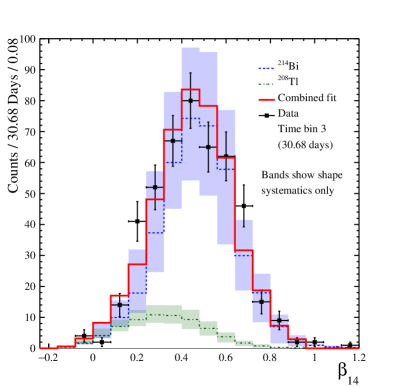
Figure 4: Data and Monte Carlo distributions of events in $\beta_{14}$ for ²¹⁴Bi and ²⁰⁸Tl decays within the AV water analysis region for data set 3. The normalizations of the Monte Carlo spectra were fit to the observed data.

V.2.2 External radioactivity

Two independent analyses were performed to measure the radioactivity from the AV, hold-down ropes and water shielding. A two-dimensional likelihood fit measured the rates of U and Th components based on $\beta_{14}$ as a function of R³—where R is the reconstructed radius of the event as measured from the center of the AV—within a background analysis region chosen to preferentially contain events from the AV, ropes and water shielding. Results from the fit analysis are shown in Table 5. ²¹⁴Bi and ²⁰⁸Tl were fit simultaneously, taking into account correlations between the two. The second analysis counted the events within four analysis regions, defined by R³ and ${\mathbb{u}}\cdot{\mathbb{r}}$ to contain events from the water within the AV, AV and ropes, water shielding and PMTs respectively. Monte Carlo simulations were used to translate the number of events observed in each into total rates and to extrapolate to the expected number of events in the ROI, shown in Table 4. The analysis took into account the correlation of events between the different regions. Bias testing of the fits ensured that asymmetries in the spatial distribution of events were properly handled. The analyses agree with each other within uncertainties.

V.2.3 PMT backgrounds

Events from radioactive decays in PMTs have a very low probability to reconstruct within the nucleon decay ROI, but occur at a very high rate, making it difficult to estimate their contribution to the total background rate using only Monte Carlo simulations. A data-driven method was used instead to put a constraint on the rate of PMT background events in the ROI. The ²⁰⁸Tl decay produces a beta particle alongside a gamma cascade that can occasionally be detected in the PMT itself. The vertex reconstruction of PMT events is dominated by the Compton scatter of the gamma while the signal from the electron will appear early and concentrated in a single PMT. Events with early hits and high charge were tagged as PMT events, with simulation studies showing a tagging efficiency of close to 30 %, while the misidentification rate is 1.4 %. The number of tagged events was used to estimate the number of expected events originating from the PMTs.

V.2.4 (alpha, n) interactions

Another potential source of background is the set of (alpha, n) reactions on ¹³C atoms within the AV itself, induced by alpha particles from the decay of ²¹⁰Po, a daughter of ²²²Rn. In about 10% of the cases, a high energy gamma or electron-positron pair is produced together with the neutron, which can act as a background for the nucleon decay search. Using predictions based on the leaching coefficient of ²¹⁰Po in water, temperature and the surface contamination on the AV Andringa et al. (2016), less than 600 (alpha, n) decays were expected during the period of data taking. Monte Carlo simulations of these events predict less than 1 event reconstructing in the nucleon decay ROI during the whole period under analysis.

V.3 Neutrino induced backgrounds

A dominant background for the nucleon decay search is the elastic scattering of ⁸B solar neutrino interactions. Such events were largely excluded by a cut on $\cos\theta_{\odot}$, the reconstructed direction relative to the direction to the Sun. Monte Carlo simulations of ⁸B solar neutrinos were constrained based on recent measurements from Super-Kamiokande Abe et al. (2016), with oscillations applied using the BS2005-OP solar model Bahcall et al. (2005).

Antineutrinos produced by nuclear reactors also contribute to the background. The expected number of events is estimated based on Monte Carlo simulations using the world reactor power data International Atomic Energy Agency (2016) with oscillations applied based on a global best fit Capozzi et al. (2016).

Atmospheric neutrino interactions can create backgrounds for the nucleon decay search, particularly through neutral-current interactions with the oxygen nuclei. The interactions can liberate a nucleon from the ¹⁶O atom, leaving either ¹⁵N* or ¹⁵O*, identical to the nucleon decay signal. However, a large fraction of these events can be tagged by looking for neutron followers appearing after the initial event. In order to estimate the size of this background, GENIE Andreopoulos et al. (2010, 2015) was used to simulate high-energy atmospheric neutrino interactions. The GENIE Monte Carlo was verified with two studies. One study counted nucleon decay-like events with neutron followers to probe the size of the neutral-current background, and a second compared the energy, time and multiplicity of Michel electron followers directly to data. Both searches found good agreement between GENIE and data and the difference between the two is used as part of the atmospheric background uncertainty estimate.

Due to the location of SNO+ at a depth of 2092 m, equivalent to close to 6000 m of water, the rate of cosmic-ray muons entering the detector is approximately three per hour. Spallation products from these cosmic-ray muons are removed by cutting all events within 20 s of a muon event, as was used during SNO. This was shown to reduce the remaining number of events from spallation products to less than one event during the data taking period Aharmim et al. (2007).

VI Analysis Methods

A blind analysis was carried out, removing events with the number of PMT hits approximately corresponding to between 5 and 15 MeV from the data set. After the analyses were finalized, blindness constraints were lifted and the whole of the data was made available for analysis.

The expected signal was simulated using Monte Carlo techniques to develop analyses that maximize the signal acceptance while minimizing the effect of backgrounds. The observables for each event used in the search were the reconstructed kinetic energy $\mathrm{T}_{e}$, the cube of the position radius R³, normalized by the cube of the radius of the acrylic vessel R${}^{3}_{AV}$, position on the z-axis of the detector z, and direction relative to the solar direction $\cos\theta_{\odot}$, as well as the event classifiers $\beta_{14}$, ITR, and ${\mathbb{u}}\cdot{\mathbb{r}}$.

Two analysis methods, a spectral analysis and, as a cross-check, a counting analysis, were used to set a limit at 90% C.I. (credibility interval) on the number of signal decays (with a prior uniform in the decay rate), $S_{90\%}$. This is then converted into a lifetime on the invisible nucleon decay modes using

$$\tau>\frac{N}{S_{90\%}}\mathrm{,}$$ (2)

where $N$ is the number of targets. For the neutron and proton modes, this is defined as the number of neutrons (or protons) in ¹⁶O atoms inside a 6 m radius in the AV, $2.41\times 10^{32}$. The difference between this 6 m radius and the fiducial radius for a particular data set is accounted for in the selection efficiency of that mode. For the dinucleon modes, $N$ is defined as the number of ¹⁶O atoms within the same volume, $3.02\times 10^{31}$.

To calculate the limit on the number of decays from the limit on the observed signal, an acceptance efficiency is calculated for each mode as the product of the theoretical branching ratios Ejiri (1993); Hagino and Nirkko (2018) and the selection efficiency from cuts on the observables with the total shown in Table 6.

Data	Signal efficiency (%)
set	$n$	$p$	$pp$	$pn$	$nn$
1	9.1 ${}^{+1.2}_{-1.2}$	11.2 ${}^{+1.1}_{-1.1}$	10.4 ${}^{+0.8}_{-0.8}$	5.9 ${}^{+0.5}_{-0.5}$	1.48 ${}^{+0.06}_{-0.06}$
2	7.5 ${}^{+0.9}_{-0.9}$	9.2 ${}^{+0.8}_{-0.9}$	8.4 ${}^{+0.6}_{-0.6}$	4.8 ${}^{+0.4}_{-0.4}$	1.19 ${}^{+0.04}_{-0.04}$
3	7.4 ${}^{+1.1}_{-1.1}$	9.3 ${}^{+1.0}_{-1.0}$	8.8 ${}^{+0.7}_{-0.7}$	5.0 ${}^{+0.4}_{-0.4}$	1.24 ${}^{+0.05}_{-0.04}$
4	7.0 ${}^{+1.1}_{-1.1}$	8.8 ${}^{+1.0}_{-1.0}$	8.3 ${}^{+0.7}_{-0.7}$	4.8 ${}^{+0.4}_{-0.5}$	1.19 ${}^{+0.05}_{-0.05}$
5	3.7 ${}^{+0.7}_{-0.6}$	4.9 ${}^{+0.6}_{-0.6}$	5.4 ${}^{+0.4}_{-0.5}$	3.1 ${}^{+0.3}_{-0.3}$	0.77 ${}^{+0.03}_{-0.03}$
6	5.2 ${}^{+1.0}_{-0.9}$	7.1 ${}^{+1.0}_{-0.9}$	7.1 ${}^{+0.7}_{-0.7}$	4.1 ${}^{+0.4}_{-0.4}$	1.09 ${}^{+0.04}_{-0.04}$

Table 6: The acceptance efficiency of the signal after applying counting analysis cuts (for both single nucleon and dinucleon decay modes) of each data set. The single nucleon decay efficiencies are given per nucleon while the dinucleon modes are given for the nucleus as a whole. Combined systematic uncertainties are given, statistical uncertainties were negligible.

VI.1 Spectral analysis

A spectral analysis was performed, fitting for the signal in the measured distribution of the observables $\bm{\eta}=[\mathrm{T}_{e},\mathrm{R}^{3},\cos\theta_{\odot},\beta_{14},{\mathbb{u}}\cdot{\mathbb{r}}]$, within the limits defined in Table 3 but with energy considered over the range 5–9 MeV for all data sets. The backgrounds in the fit included solar neutrinos, reactor neutrinos and atmospheric neutrinos as well as radioactivity from U and Th chain decays in the water, AV, ropes, water shielding and PMTs. Probability distributions for the signal and backgrounds, $\mathcal{P}_{s}(\bm{\eta}_{i})$ and $\mathcal{P}_{b}(\bm{\eta}_{i})$, were generated using Monte Carlo simulations with constraints on the radioactive backgrounds provided by the likelihood-fit external analysis.

To allow for the multiple data sets, the analysis simultaneously maximized the sum of the log likelihoods of each individual data set $k$, as described by:

$$\begin{aligned} &-\ln\mathcal{L}(s,\bm{\beta}|\bm{\eta},\hat{\bm{\beta}},\bm{\sigma},t_{k})=\\ &-\sum_{k}\sum_{i=1}^{n_{obs}}\ln\biggl{\{}s\epsilon_{s,k}\mathcal{P}_{s,k}(\bm{\eta}_{i})+\sum_{b}\beta_{b,k}\epsilon_{b,k}\mathcal{P}_{b,k}(\bm{\eta}_{i})\biggr{\}}t_{k}\\ &+\sum_{k}\biggl{(}s\epsilon_{s,k}+\sum_{b}\beta_{b,k}\epsilon_{b,k}\biggr{)}t_{k}+\sum_{k}\sum_{b}\frac{(\beta_{b,k}-\hat{\beta}_{b,k})^{2}}{2\sigma_{b,k}^{2}}\mathrm{,}\end{aligned}$$ (3)

where $n_{obs}$ is the number of observed events in each data set, $s$ is the signal decay rate, $\epsilon_{s,k}$ is the acceptance efficiency of the signal in data set $k$, $\beta_{b}$ is the rate of background component $b$ whose expectation $\hat{\beta}_{b}$ is constrained by $\sigma_{b}$, $\epsilon_{b}$ is the acceptance efficiency for the background $b$ and $t_{k}$ is the live time of data set $k$. Fits were bias tested using a sampling of fake data sets based on Monte Carlo simulations.

To find $S_{90\%}$, a profile likelihood Tanabashi et al. (2018) distribution is calculated by taking the value of the maximum likelihood for a given value of $s$. The upper limit at 90% C.I. is then found by integrating along this distribution.

VI.2 Counting analysis

A counting experiment with a set of rigid cuts, shown in Table 3, is also used, where the number of background events is calculated directly from the background analyses and is shown in Table 4. Due to changes in the level of backgrounds, candidate events were selected using different cuts during different periods of running. The signal acceptance within each data set is shown in Table 6. Using a Bayesian method Helene (1983), an upper limit on the number of signal decays that could have occurred is found by numerically solving

$$\int\limits^{S_{90\%}}_{0}\prod_{k}A\biggl{(}s\epsilon_{k}t_{k}+b_{k}\biggr{)}^{n_{k}}\times\mathrm{e}^{-\left(s\epsilon_{k}t_{i}+b_{k}\right)}\mathrm{d}s/n_{k}!=0.9\mathrm{,}$$ (4)

where $S_{90\%}$ is the upper limit on the number of signal decays at 90% credibility level and, for each data set $k$, $b_{k}$ is the number of expected background events, combined from internal and external radioactivity, solar, reactor, atmospheric and instrumental backgrounds, $n_{k}$ is the number of observed events while $\epsilon_{k}$ and $t_{k}$ are the signal efficiency after cuts and the live time of the data set. $A$ is a normalization factor such that the integral tends to 1 as $S_{90\%}$ tends to infinity.

VII Results

The results of the spectral analysis for the neutron decay mode are shown in Fig. 5 with the fitted energy spectrum of the neutron decay signal at its maximum likelihood value plotted alongside the fitted backgrounds and data. Figure 6 shows the normalized and cumulative likelihood distribution for the neutron mode. The resulting limits on each mode of invisible nucleon decay are shown in Table 7 alongside the existing limits. A breakdown of systematic uncertainties is given in Table 8.

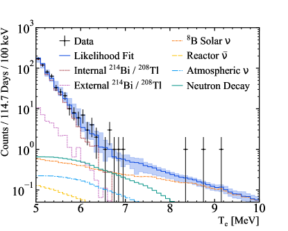
Figure 5: Fitted energy spectrum across all data sets for neutron decay and backgrounds. Backgrounds were fit for each data set and the spectrum shown is the sum over all of the time-bins for the individual components. The contributions of Bi and Tl were fit independently for internal backgrounds but were merged in this plot. The signal is shown at its maximum likelihood, not at 90% C.I. The errors around the full fit include the MC statistical uncertainties summed in quadrature with the individual systematic uncertainties. These errors are bin-by-bin correlated and are dominated by the energy resolution and the energy scale systematic uncertainties.

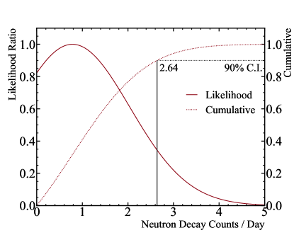
Figure 6: The likelihood ratio (the maximum likelihood as a function of the signal divided by the likelihood at the best fit value) for the neutron decay mode of the spectral analysis versus the limit of the number of signal decays per day. The associated cumulative distribution indicates the point at which the limit on the signal at 90% C.I. is drawn.

	Spectral analysis	Counting analysis	Existing limits
$n$	$2.5\times 10^{29}$ y	$2.6\times 10^{29}$ y	$5.8\times 10^{29}$ y Araki et al. (2006)
$p$	$3.6\times 10^{29}$ y	$3.4\times 10^{29}$ y	$2.1\times 10^{29}$ y Ahmed et al. (2004)
$pp$	$4.7\times 10^{28}$ y	$4.1\times 10^{28}$ y	$5.0\times 10^{25}$ y Back et al. (2003)
$pn$	$2.6\times 10^{28}$ y	$2.3\times 10^{28}$ y	$2.1\times 10^{25}$ y Tretyak et al. (2004)
$nn$	$1.3\times 10^{28}$ y	$0.6\times 10^{28}$ y	$1.4\times 10^{30}$ y Araki et al. (2006)

Table 7: Lifetime limits at 90% C.I. for the spectral and counting analysis, including statistical and systematic uncertainties alongside the existing limits.

Systematic	$n$ (events/day)	$p$ (events/day)	$pp$ (events/day)	$pn$ (events/day)	$nn$ (events/day)
Best fit	0.66	0.55	0.57	0.99	2.34
Energy scale	+0.42, $-0.21$	+0.25, $-0.13$	+0.21, $-0.12$	+0.41, $-0.23$	+0.53, $-0.28$
Energy resolution	$\pm 1.01$	$\pm 0.67$	$\pm 0.60$	$\pm 1.11$	$\pm 1.20$
x-shift	$\pm 0.02$	$\pm 0.01$	$\pm 0.01$	$\pm 0.02$	$\pm 0.02$
y-shift	$\pm 0.01$	$\pm 0.01$	$\pm 0.01$	$\pm 0.02$	$\pm 0.03$
z-shift	+0.02, $-0.01$	+0.01, $-0.01$	+0.01, $-0.01$	+0.03, $-0.01$	+0.05, $-0.01$
xyz-scale	+0.14, $-0.13$	+0.10, $-0.09$	+0.10, $-0.08$	+0.19, $-0.16$	+0.31, $-0.25$
$\beta_{14}$	$\pm 0.04$	$\pm 0.03$	$\pm 0.03$	$\pm 0.07$	$\pm 0.14$
Direction	+0.14, $-0.07$	+0.11, $-0.07$	+0.11, $-0.08$	+0.21, $-0.13$	+0.44, $-0.28$
Total (syst.)	+1.12, $-1.05$	+0.73, $-0.69$	+0.65, $-0.62$	+1.22, $-1.15$	+1.43, $-1.30$
Statistical	+0.57, $-0.48$	+0.42, $-0.37$	+0.42, $-0.40$	+0.75, $-0.71$	+2.16, $-1.59$
90% C.I.	2.64	1.85	1.76	3.21	6.59

Table 8: Systematic uncertainties and fit results for the spectral analysis. For each of the decay modes, the best fit is given as well as the difference between the best fit and the shift-and-refit value for each source of uncertainty. The total is the sum in quadrature of each of the separate systematic uncertainties assuming no correlation between the components. The statistical uncertainty, found by integrating the likelihood function prior to convolution with the systematic uncertainties using a Feldman-Cousins confidence interval to 1$\sigma$, is shown for comparison. Finally, the convolved likelihood function is integrated to 90% to get the final limit shown on the last line.

Data	Observed	Expected
set	events	events
1	1	1.17${}^{+4.60}_{-0.05}$ ${}^{+1.33}_{-0.39}$
2	2	2.35${}^{+4.62}_{-0.40}$ ${}^{+3.44}_{-0.81}$
3	4	3.47${}^{+4.60}_{-0.15}$ ${}^{+3.11}_{-0.96}$
4	8	3.37${}^{+4.60}_{-0.17}$ ${}^{+2.70}_{-0.98}$
5	1	1.46${}^{+4.60}_{-0.13}$ ${}^{+2.17}_{-0.60}$
6	6	5.84${}^{+7.40}_{-2.31}$ ${}^{+2.68}_{-0.62}$
Total	22	17.65${}^{+12.68}_{-2.36}$ ${}^{+6.51}_{-1.85}$

Table 9: The observed and predicted number of events passing the counting analysis cuts for each data set. The uncertainty on the total number is found by treating each data set as independent and combining in quadrature. The first uncertainty is the statistical uncertainty, the second is the total systematic uncertainty. The statistical uncertainty is almost completely dominated by the background from the PMTs.

Systematic	$n$ (events/day)	$p$ (events/day)	$pp$ (events/day)	$pn$ (events/day)	$nn$ (events/day)
Energy resolution	0.72	0.54	0.52	0.92	4.07
Energy scale	0.42	0.26	0.24	0.43	0.87
Position resolution	0.11	0.09	0.09	0.16	0.63
Position shift	0.02	0.01	0.01	0.02	0.09
Position scale	0.03	0.03	0.03	0.05	0.18
Direction resolution	0.03	0.03	0.03	0.05	0.19
$\beta_{14}$	0.04	0.03	0.03	0.06	0.24
Trigger efficiency	0.03	0.02	0.02	0.04	0.16
Instrumentals	0.04	0.03	0.04	0.06	0.25
Total systematic	0.84	0.61	0.58	1.03	4.24
Statistics	0.30	0.24	0.25	0.44	1.81

Table 10: Systematic uncertainties for the counting analysis on the upper limit (at 90% C.I.) on the signal decays per day, shown as the difference to the unshifted value.

For the counting analysis, Table 9 shows the observed events compared to the predictions for each data set. The results of the counting analysis are shown alongside those of the spectral analysis in Table 7. A breakdown of the systematic uncertainties is shown in Table 10.

VIII Conclusion

The results shown by the spectral and counting analyses in Table 7 are in good agreement. In the case of the dineutron decay mode, the spectral analysis performed significantly better due to the difference in the spectral shape of the dineutron signal, which is not taken into account within the counting analysis.

The limit set in this work on the lifetime of the proton decay mode of 3.6$\times 10^{29}$ y is an improvement on the existing limit from SNO, however the neutron mode limit of 2.5$\times 10^{29}$ y is weaker than the current limit from KamLAND.

For the dinucleon modes, the $nn$ limit of 1.3$\times 10^{28}$ y does not improve upon the existing limit set by KamLAND, but the $pn$ and $pp$ mode limits of 2.6$\times 10^{28}$ y and 4.7$\times 10^{28}$ y improve upon the existing limits by close to three orders of magnitude.