Structure and dynamics in low density regions: galaxy-galaxy correlations inside cosmic voids

Abstract

We compute the galaxy-galaxy correlation function of low-luminosity SDSS-DR7 galaxies $(-20<M_{\rm r}-5\log_{10}(h)<-18)$ inside cosmic voids identified in a volume limited sample of galaxies at $z=0.085$. To identify voids, we use bright galaxies with $M_{\rm r}-5\log_{10}(h)<-20.0$. We find that structure in voids as traced by faint galaxies is mildly non-linear as compared with the general population of galaxies with similar luminosities. This implies a redshift-space correlation function with a similar shape than the real-space correlation albeit a normalization factor. The redshift space distortions of void galaxies allow to calculate pairwise velocity distributions which are consistent with an exponential model with a pairwise velocity dispersion of $w\sim 50-70{\rm~{}km/s}$, significantly lower than the global value of $w\sim 500{\rm~{}km/s}$. We also find that the internal structure of voids as traced by faint galaxies is independent of void environment, namely the correlation functions of galaxies residing in void-in-void or void-in-shell regions are identical within uncertainties. We have tested all our results with the semi-analytic catalogue MDPL2-Sag finding a suitable agreement with the observations in all topics studied.

1 Introduction

The large-scale structure of the Universe can be understood as a complex net of filaments and plane structures of dark matter which intersect forming massive virialized systems, regions of preferred galaxy formation. As a result, between these structures, large-scale underdense regions emerge, known as cosmic voids. Depending on the identification algorithm, several properties such as topology and fraction of mass or galaxies inside the voids can significantly vary (Colberg et al., 2008; Cautun et al., 2018). One of the simplest way to define cosmic voids is to considerer them as expanding spherical regions with 10 to 20 percent of the mean density of the Universe (Padilla et al., 2005; Ceccarelli et al., 2006; Ruiz et al., 2015).

Observationally, galaxies residing cosmic voids have been studied from different point of views and in several galaxy catalogues. By construction, voids lack a significant fraction of luminous galaxies, and so their inner structure can be traced by faint objects (Lindner et al., 1996; Alpaslan et al., 2014). It should be noticed that, induced by void expansion, galaxies residing voids can perceive a local Hubble constant larger than the average (Tomita, 2000). Both the large local Hubble constant and a the low mass density conspire against structure growth which is expected to be significantly lower than elsewhere, providing the galaxies that populate voids very different astrophysical and dynamical properties compare to those in higher density regions. Regarding to their photometric properties, void galaxies tend to be fainter, bluer and late-type (Rojas et al., 2004; Hoyle et al., 2005; Patiri et al., 2006; Ceccarelli et al., 2008; Hoyle et al., 2012). Also, the spectroscopic properties of galaxies within voids show younger stellar populations and higher star formation rates (Rojas et al., 2005). All these properties depend on the emptiness of the host void as well (Tavasoli et al., 2015).

The inner structure of cosmic voids has also been studied with detail in numerical simulations by Gottlöber et al. (2003) and Aragon-Calvo & Szalay (2013), unveiling the complex structure traced by galaxies in these underdense regions. In this paper we address the two-point correlation function and derive pairwise velocitiy distributions of faint galaxies within voids, both in observations and in a cosmological simulation with a semi-analytic model implementation.

It should be noticed that faint galaxies in rich clusters type environments behave in a similar fashion than luminous ones since the dynamics is globally dominated by the cluster potential. By contrast, inside voids, no rich clusters are expected, so that the dynamics of faint galaxies may reflect more faithfully initial conditions unaffected by induced strongly non-linear peculiar motions.

This paper is organized as follows. In Sec. 2 we describe the observed and simulated galaxy catalogues used. In Sec. 3 we present the results of redshift and real-space inferred two point correlation functions for galaxies inside voids and compare to the global results. In Sec. 4 we analyse the corresponding 2D correlation function $\xi(\sigma,\pi)$ and derive pairwise velocity distributions. We also compare in Sec. 5, the possible clustering dependence on global void environment. The results obtained are listed in Sec. 6.

2 Data

In this section we present both the observational and the simulated galaxy catalogues used in this work. Also, we describe the void identification procedure and the derived void catalogues.

2.1 Observed galaxies

We use the Main Galaxy Sample of the Sloan Digital Sky Survey Data Release 7 (SDSS-DR7, York et al., 2000; Strauss et al., 2002; Abazajian et al., 2009), which comprises nearly a millon galaxies up to $z\sim 0.3$ with an upper limiting apparent magnitude in the $r$-band $m_{r}^{\rm lim}=17.77$. From this catalogue, we select all galaxies with $r$-band magnitudes $14.5\leq m_{\rm r}\leq 17.77$ in the redshift range $0.02\leq z\leq 0.085$, comprising a total of approximately $2.5\times 10^{5}$ galaxies.

2.2 Simulated galaxies

The simulated semianalytic galaxies used in our analysis were extracted from the public release MultiDark-Galaxies (Knebe et al., 2018), available at the CosmoSim database. Specifically, we use the catalogue MDPL2-Sag, which is derived by populating the dark matter haloes of the MDPL2 simulation using the semi-analytic model of galaxy formation and evolution Sag (Cora et al., 2018).

The MDPL2 simulation belongs to the MultiDark suite of simulations (Riebe et al., 2013; Klypin et al., 2016) and is also available at the CosmoSim database. This simulation follows the evolution of $3840^{3}$ dark matter particles in a cubic comoving box of $1000h^{-1}{\rm Mpc}$ on a side. The adopted cosmology is a flat $\Lambda$CDM with cosmological parameters: $\Omega_{\rm m}=0.307$, $\Omega_{\rm\Lambda}=0.693$, $\Omega_{\rm b}=0.048$, $\sigma_{8}=0.823$, $n=0.96$ and $h=0.678$, consistent with Planck results (Planck Collaboration et al., 2014, 2016). The dark matter haloes have been identified with Rockstar (Behroozi et al., 2013a), finding $\sim 127\times 10^{6}$ haloes with at least 20 particles, and the merger trees were constructed using ConsistentTrees (Behroozi et al., 2013b).

The Sag model includes most of the relevant physical processes in galaxy formation and evolution, such as radiative cooling of hot gas, star formation, feedback from supernova explosions, chemical enrichment, growth of supermassive black holes, AGN feedback and starburst via disc instabilities and galaxy mergers. This model was calibrated to generate a galaxy catalogue using the MDPL2 simulation, which together with the catalogues constructed using Sage (Croton et al., 2016) and Galacticus (Benson, 2012), conform the MultiDark-Galaxies database previously mentioned.

The complete MDPL2-Sag catalogues has $\sim 194\times 10^{6}$ galaxies at $z=0$, although we keep only those galaxies with $r$-band absolute magnitudes in the range $M_{\rm r}-5\log_{10}(h)\leq-16.0$ and stellar masses $M_{\star}\geq 10^{8}h^{-1}{\rm M}_{\odot}$, nearly $91\times 10^{6}$ simulated galaxies.

2.3 Void catalogues and void galaxies

In order to identify voids both in the SDSS-DR7 and MDPL2-Sag catalogues, we use the algorithm described in Ruiz et al. (2015). Briefly, the algorithm starts with a Voronoi tessellation (Voronoi, 1908) of the density field, using galaxies as tracers. Each Voronoi cell has an associated density which is given by the inverse of the cell volume, $\rho_{\rm cell}=1/V_{\rm cell}$. Defining the density contrast as

$$\delta=\frac{\rho_{\rm cell}}{\bar{\rho}}-1,$$ (1)

where $\bar{\rho}$ is the mean density of tracers, we select any Voronoi cell with $\delta<-0.8$ as a center of an underdense region. From theses centers, we select as void candidates all spherical volumes with an integrated density contrast which satisfy

$$\Delta(R_{\rm void})=\frac{3}{R^{3}_{\rm void}}\int_{0}^{R_{\rm void}}\delta(r)r^{2}dr<-0.9,$$ (2)

where $R_{\rm void}$ is the void radius. Once these void candidates are identified, we repeat the computation of $\Delta$ in a randomly displaced center around the previous one, where these are only accepted if the new $R_{\rm void}$ is larger than the previous one. This procedure is repeated several times, mimicking a random walk around the original center, alloing to obtain void candidates with centers located in the true local minima of the density field. Finally, the void catalogue is formed by the largest void candidates which do not overlap with any other void candidate.

In the case of the SDSS-DR7 sample, we select all galaxies with absolute magnitudes in the $r$-band brighter than $M_{\rm r}-5\log_{10}(h)=-20.0$ (the limiting magnitude for a complete volume limited sample at $z=0.085$ is $M_{\rm r}-5\log_{10}(h)=-19.4$). This subsample of $\sim 7.3\times 10^{4}$ galaxies, which corresponds to a galaxy volume number density of $n=6.4\times 10^{-3}$, was used as tracers to identify spherical cosmic voids, obtaining $167$ voids with radii in the range $7-24h^{-1}{\rm Mpc}$. Void identification procedure considers a HEALPix (Górski et al., 2005) angular mask of the SDSS-DR7 that takes into account catalogue boundaries and holes within the survey. It is important to note that we only consider those voids which do not include any boundary of the catalogue. Finally, we consider all galaxies in SDSS-DR7 in the redshift range $0.02\leq z\leq 0.085$ and $-18.0\geq M_{\rm r}-5\log(h)\geq-20.0$ in order to populate the voids with low luminosity galaxies.

For the MDPL2-Sag catalogue, to identify voids comparable to those identified in the SDSS-DR7 data, we construct a subsample of galaxies with the same volume density than in the SDSS-DR7 by selecting all galaxies brighter than $M_{\rm r}-5\log(h)=-20.6$. This cut is different than that used in SDSS-DR7 mainly due to the differences in the luminosity functions of observations and simulations. Voids identified in the full MDPL2 box with the same volume density of tracers have the same radii range than those identified in the SDSS-DR7, allowing us a proper comparison between both datasets. In order to take into account redshift-space distortions, the 3D positions of simulated galaxies were transformed to redshift-space by affecting the z-coordinate by peculiar velocities, z${}_{\rm redshift-space}={\rm z}+v_{\rm z}/100h^{-1}$, where $v_{\rm z}$ is the z-component of the peculiar velocity of the galaxy. This subsamble comprises $6.4\times 10^{6}$ galaxies, and we use it to identify $17694$ voids with the same radii range than those in the SDSS-DR7. To populate these voids with low luminosity galaxies, we consider all galaxies in the catalogue with $-18.6\geq M_{\rm r}-5\log(h)\geq-20.6$.

Fig. 1 show the normalized void radius distributions from both simulated and observed catalogues. The distribution for voids identified in MDPL2-Sag catalogue is plotted with the solid black line, and the one corresponding to SDSS-DR7 voids whit the grey shaded histogram. Error bars correspond to Poisson uncertainties in both cases.

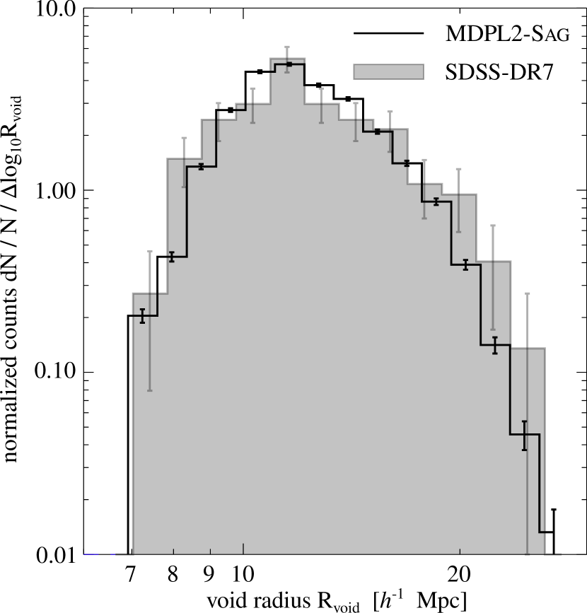
Figure 1: Normalized number counts of voids as a function of void radius. The distribution for MDPL2-Sag voids are shown with black solid line and for SDSS-DR7 voids with the grey shaded area. In both cases, error bars correspond to Poisson uncertainties.

3 The two-point galaxy-galaxy correlation function

3.1 Redshift and real-space correlation functions

We compute the redshift-space correlation functions, $\xi(s)$, we using the classical estimator of Davis & Peebles (1983),

$$\xi(s)=\frac{DD(s)}{DR(s)}\frac{N_{\rm R}}{N_{\rm D}}-1,$$ (3)

where $N_{\rm D}$ is the number of galaxies, $N_{\rm R}$ is the number of random tracers, $DD$ is the number of galaxy-galaxy pairs and $DR$ is the number of galaxy-random tracer pairs. We have also tested other estimators finding similar results. .

For both galaxy catalogues (observed and simulated), we compute $\xi(s)$ for two samples: (i) galaxies inside cosmic voids, namely void galaxies, and (ii) galaxies in the full catalogue, namely all galaxies. For sample (i) we stack all pairs of galaxies in all voids into one measure of $\xi(s)$. We use random distributions of tracers in spheres centered in voids with the same radii, so we take into account border effects in the computation of $DR$ pairs consistent with the distribution of galaxies constrained to reside in cosmic voids. We also compute $\xi(s)$ for sample (ii) where the galaxies have the same magnitude distribution of void galaxies, allowing for a fair comparison between these two equal-luminosity galaxy samples.

In the case of SDSS-DR7 catalogue, the unclustered random distribution of tracers is generated using the method presented in Cole (2011) within the SDSS-DR7 mask. In order to compute $\xi(s)$ for void galaxies we use a distribution of random tracers with spherical distributions that fill the void volumes. For MDPL2-Sag catalogue, the number of $DR$ pairs for all galaxies can be computed analytically, whereas for void galaxies we use random distributions inside spheres of the same distribution of void radii and with the same number density of tracers.

The real-space correlation function, $\xi(r)$, for SDSS-DR7 galaxies was derived from the redshift-space counterpart by applying the inversion method presented by Saunders et al. (1992). In this method, the real-space correlation function can be computed using the projected correlation function $\Xi(\sigma)$ (see Sec 4.2) through

$$\xi(r_{i})=-\frac{1}{\bar{\pi}}\sum_{j\geq i}\frac{\Xi_{j+1}-\Xi_{j}}{\sigma_{j+1}-\sigma_{j}}\ln\left(\frac{\sigma_{j+1}+\sqrt{\sigma_{j+1}^{2}+\sigma_{i}^{2}}}{\sigma_{j}+\sqrt{\sigma_{j}^{2}-\sigma_{i}^{2}}}\right)$$ (4)

where $r_{i}=\sigma_{i}$, $\Xi_{i}=\Xi(\sigma_{i})$ and $\bar{\pi}=3.14159...$, to distinguish it from $\pi$, the line-of-sight component of the galaxy-galaxy distance we will introduce in Sec. 4. For MPDL2-Sag galaxies, $\xi(r)$ is directly measured from the simulated catalogue.

3.2 Results for SDSS-DR7 and MDPL2-Sag galaxies

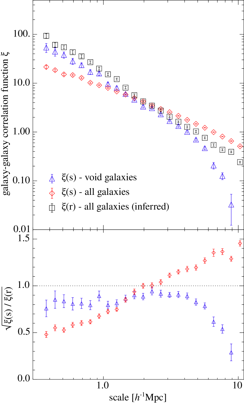
Figure 2: Top panel: Galaxy-galaxy correlation function in the SDSS-DR7 catalogue. Blue triangles represent the redshift-space correlation functions $\xi(s)$ for galaxies inside voids stacked for all the voids, meanwhile the red diamonds show the $\xi(s)$ for all galaxies in the catalogue with the same luminosity distribution than galaxies inside voids. Black squares show the real-space $\xi(r)$ correlation function for all galaxies obtained via the inversion of $\Xi(\sigma)$ (Saunders et al., 1992). Errors represent the variance in galaxy pairs estimated using Jackknife resampling. Bottom panel: ratio between redshift and real-space correlations defined as $\sqrt{\xi(s)/\xi(r)}$. Errors were obtained with error propagation.

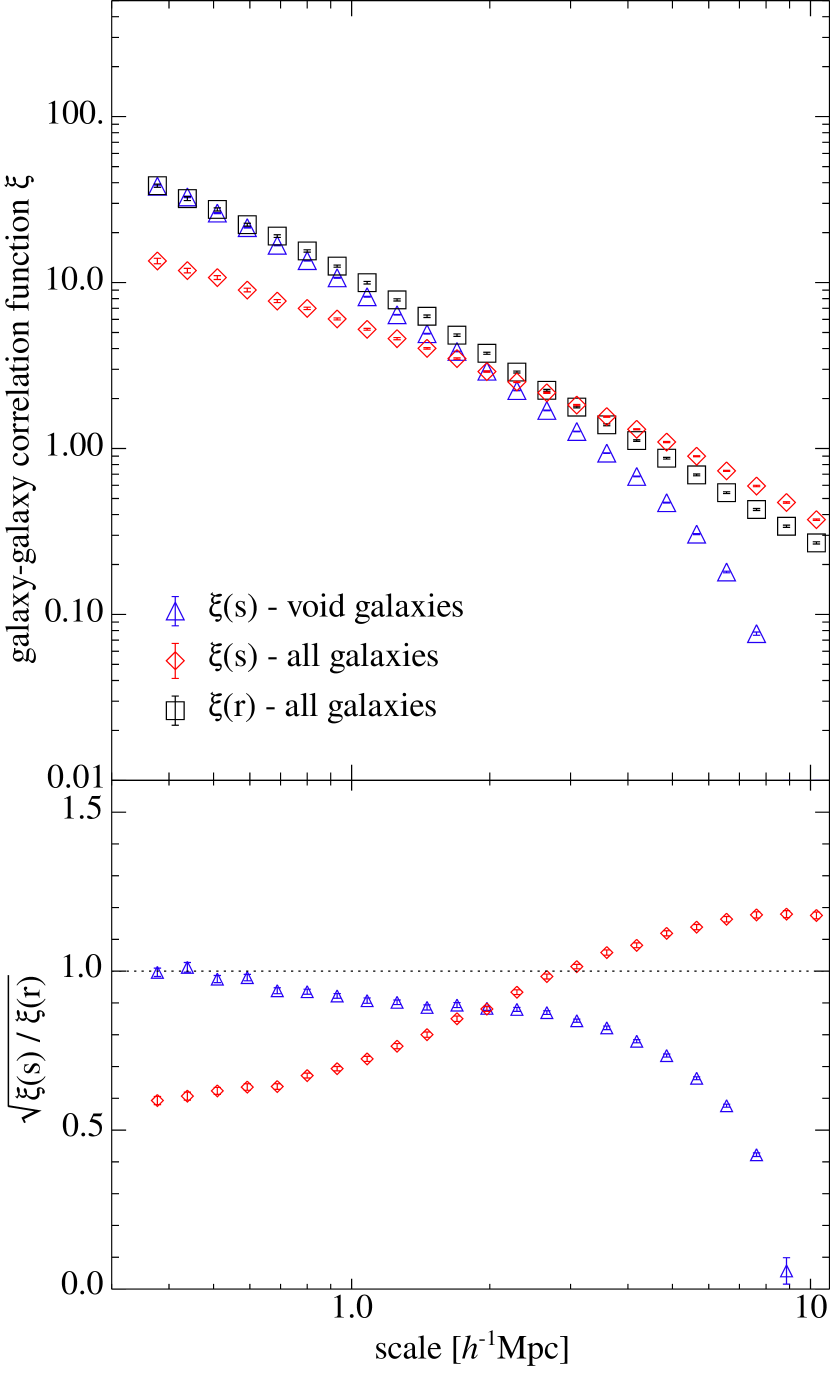
Figure 3: Same as Fig. 2 but for the MDPL2-Sag catalogue. The only difference is that in this case $\xi(r)$ can be computed directly from the simulated galaxies unaffected by peculiar velocities distortions.

In Fig. 2 we show the real-space $\xi(r)$ and redshift-space $\xi(s)$ two point galaxy correlation functions computed for SDSS-DR7. In the upper panel are given the resulting $\xi(s)$ for all galaxies (red diamonds) and for galaxies in voids (blue triangles). The black squares correspond to $\xi(r)$ for all galaxies inferred via Eq. (4). In all cases, the errorbars represent the uncertainties estimated via Jackknife resampling (Efron, 1982) in galaxy pairs. As it can be seen in this panel, at small scales ($r<5h^{-1}{\rm Mpc}$) the shape of the real-space correlation function of the global population differs significantly from the corresponding redshift-space function while on the contrary, galaxies in cosmic voids have redshift-space correlation function remarkably close to the real-space measures. This is more clearly shown in the bottom panel of this figure where the ratio between redshift and real-space correlation functions, defined as $\sqrt{\xi(s)/\xi(r)}$, for void galaxies is nearly constant at $\sim$ $0.8$ in the range $0.3-3.0h^{-1}{\rm Mpc}$. By contrast, in this same range of separations, the ratio for the global population changes by a factor larger than $2$.

The corresponding results for the semi-analytic model MDPL2-Sag are shown in Fig. 3. Again, $\xi(s)$ for all galaxies is shown in red diamonds, and for galaxies in voids, in blue triangles. The resulting $\xi(r)$ for all galaxies, shown with black squares, is computed directly form the MDPL2-Sag galaxies unaffected by peculiar velocities. As it can be seen here, the results are remarkably similar although with lower errorbars due to the significantly larger number of semi-analytical galaxies and voids. In the case of MDPL2-Sag, the ratio $\sqrt{\xi(s)/\xi(r)}$ is also approximately constant in the range $0.3-3.0h^{-1}{\rm Mpc}$, while the global one also changes by a factor $\sim$ 2.

As can be seen in Figs. 2 and 3, $\xi(s)$ for void galaxies depart from a power-law behavior for scales $s>3.0h^{-1}{\rm Mpc}$. This in consistent with the absence of a significant two-halo term in the galaxy-galaxy correlations inside voids due to the lack of massive haloes associated to bright galaxies. Given the void radii distributions (see Fig. 1), galaxy-galaxy correlations are well determined up to scales of $\sim 10h^{-1}{\rm Mpc}$, the maximum scale shown in these figures.

It is also important to note in Fig. 3 the lack of power of $\xi(r)$ for $r<1h^{-1}{\rm Mpc}$, a feature that can be understood due to orphan galaxies in semi-analytical models. Orphan galaxies are galaxies which can not retain their host subhaloe, a phenomenon that can occur by physical mechanism such as tidal stripping, or just by resolution limitations in the subhaloe identification (Onions et al., 2012). The treatment of this particular type of galaxies differs from model to model (Knebe et al., 2015), having an impact in the galaxy-galaxy correlation function at small scales (Pujol et al., 2017; Knebe et al., 2018). The Sag model used in this work considers the orphan galaxies, deriving their positions and velocities from an orbital integration. This treatment allows to obtain an adequate radial distribution of satellite galaxies, however, it does not trace faithfully the spatial distribution of the true population of faint galaxies, a fact that is expected to be particularly serious in high density regions where nonlinearities dominate the dynamics. Inside cosmic voids, however, these effects are expected to be less important given that the dynamical behaviour of galaxies in regions lacking strong mass concentrations is expected to be only mildly non-linear.

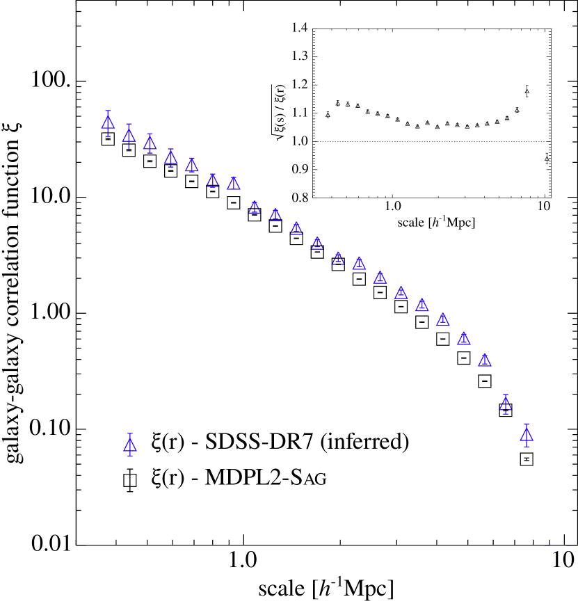
Figure 4: Galaxy-galaxy correlation functions of void galaxies in real-space for the MDPL2-Sag (black squares) and for the SDSS-DR7 (blue triangles). The inset figure shows the ratio $\sqrt{\xi(s)/\xi(r)}$ measured for MDPL2-Sag void galaxies, which was used to infer $\xi(r)$ for SDSS-DR7 void galaxies (see text for details). Errorbars correspond to Jackknife estimations of the uncertainties.

In Fig. 4 we show the real-space correlation function $\xi(r)$ for MDPL2-Sag (direct measure) with black squares and that derived for void galaxies SDSS-DR7 with blue triangles. We notice that the real-space $\xi(r)$ for SDSS-DR7 void galaxies obtained by the direct inversion of Eq. (4) is noisy given the low number statistics with respect to the MDPL2-Sag void galaxies. Therefore, we assume the same ratio between $\xi(r)$ and $\xi(s)$ of the simulations to infer the spatial correlation function $\xi(r)$ of SDSS-DR7 from the corresponding redshift-space $\xi(s)$ determination. We notice that the inferred $\xi(r)$ by this method is entirely consistent with that derived by direct inversion using Eq. (4), albeit much smoother. This ratio is shown in the inset of Fig. 4. By inspection to this figure it can be seen a very suitable agreement of the two measures showing that, inside voids, the distribution of MDPL2-Sag faint galaxies is in agreement with that observed in the SDSS-DR7 data.

	MDPL2-Sag	MDPL2-Sag	SDSS-DR7	SDSS-DR7
	all galaxies	void galaxies	all galaxies	void galaxies
$r_{0}$	$4.5\pm 0.1$	$3.3\pm 0.1$	$4.8\pm 0.1$	$3.9\pm 0.1$
$\gamma$	$1.60\pm 0.02$	$1.66\pm 0.03$	$1.78\pm 0.02$	$1.65\pm 0.03$

Table 1: Autocorrelation function $\xi(r)$ power-law fitting parameters. For galaxies in voids, we restrict the fit to measurements in the range $0.3-3.0h^{-1}{\rm Mpc}$.

In Tab. 1 we show the fitting parameters obtained by modeling the real-space correlation function with a power-law of the form

$$\xi(r)=\left(\frac{r}{r_{0}}\right)^{-\gamma}$$ (5)

We adopt the range $0.3-10h^{-1}{\rm Mpc}$ for all galaxies, and use a more restricted range of $0.3-3.0h^{-1}{\rm Mpc}$ for galaxies in voids to avoid border effects. The purpose of these fits are mainly to provide simple theoretical models for the 2D correlation function $\xi(\sigma,\pi)$ and the derivation of the pairwise velocity distribution $f(v)$ presented in the next section.

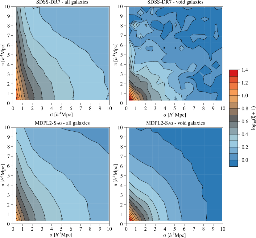
Figure 5: 2D galaxy-galaxy correlation function $\xi(\sigma,\pi)$ for SDSS-DR7 (upper panels) and MDPL2-Sag (bottom panels) galaxies. For both catalogues, the results for all galaxies are shown in left panels, meanwhile in the right panels are the results for void galaxies. Contours show the different values of $\log_{10}(\xi+1)$ as indicated in the legends and colour bar.

4 $\xi(\sigma,\pi)$ and derivation of pairwise velocity distributions

We have also computed the 2D galaxy-galaxy correlation function in the form $\xi(\sigma,\pi)$, where $\sigma$ and $\pi$ are the projected and line-of-sight components of the galaxy-galaxy pair distance, respectively.

In Fig. 5 we show the $\xi(\sigma,\pi)$ correlation functions computed for the SDSS-DR7 (upper panels) and MDPL2-Sag (bottom panels). In both cases, left panels correspond to $\xi(\sigma,\pi)$ measured in all galaxies and right panels to the measurements for void galaxies. By inspection to these figures it can be seen a general agreement between simulated and observational data. As seen in Figs. 2 and 3, galaxies within voids present much less distortions due to Finger-of-God effect than in the global population.

The information contained in these correlation functions can be used to estimate galaxy pairwise velocity distributions, $f(v)$, to have more insight in the dynamical properties of galaxies inside cosmic voids. In the next subsections we describe the procedures to measure and estimate $f(v)$ from $\xi(\sigma,\pi)$.

4.1 Measuring $f(v)$

In order to determine the pairwise velocity distributions of both SDSS-DR7 and MDPL2-Sag catalogues, we use the projections of the correlation functions, $\Xi$, onto the $\sigma$ and $\pi$ axes

$$\Xi_{\sigma}=\Xi(\sigma)=2\int_{0}^{\pi_{\rm lim}}\xi(\sigma,\pi)d\pi$$ (6)

$$\Xi_{\pi}=\Xi(\pi)=2\int_{0}^{\sigma_{\rm lim}}\xi(\sigma,\pi)d\sigma$$ (7)

where $\sigma_{\rm lim}=\pi_{\rm lim}=20h^{-1}{\rm Mpc}$. The projected correlation function $\Xi_{\sigma}$ is not affected by redshift space distortions induced by pairwise velocities, meanwhile the projection $\Xi_{\pi}$ arises from a convolution with the pairwise velocity distribution. We take the Fourier transform $(\mathcal{F})$ of $\Xi_{\sigma}$ and $\Xi_{\pi}$, and take advantage of the fact than a convolution is just a multiplication in Fourier-space to recover the pairwise velocity distribution:

$$f(v)=\mathcal{F}^{-1}\left[\frac{\mathcal{F}[\Xi_{\pi}]}{\mathcal{F}[\Xi_{\sigma}]}\right]$$ (8)

4.2 Modeling $f(v)$

To model the velocity distributions $f(v)$ and obtain an estimation for the mean pairwise velocity dispersion $w=\langle\sigma_{v}^{2}\rangle^{1/2}$, we follow the method described in Hawkins et al. (2003).

We start with a model of $\xi_{\rm K}(\sigma,\pi)$ which takes into account the coherent infall velocities (Kaiser, 1987; Hamilton, 1992)

$$\xi_{\rm K}(\sigma,\pi)=\sum_{i=0,2,4}\xi_{i}(s)P_{i}(\cos{\theta})$$ (9)

where $P_{i}(x)$ are the Legendre polynomials and $\theta$ is the angle between $r$ and $\pi$. If we asume a power law for $\xi(r)$ of the form given by Eq. (5), the relations between $\xi_{i}(s)$ and $\xi(r)$ are given by

$$\xi_{0}(s) = \left(1+\frac{2\beta}{3}+\frac{\beta^{2}}{5}\right)\xi(r)$$ (10)

$$\xi_{2}(s) = \left(\frac{4\beta}{3}+\frac{4\beta^{2}}{7}\right)\left(\frac{\gamma}{\gamma-3}\right)\xi(r)$$ (11)

$$\xi_{4}(s) = \frac{8\beta^{2}}{35}\left(\frac{\gamma(2+\gamma)}{(3-\gamma)(5-\gamma)}\right)\xi(r)$$ (12)

where

$$\beta=\frac{f(\Omega)}{b}\simeq\frac{\Omega_{\rm m}^{0.6}}{b}$$ (13)

is the parametrization of the large-scale coherent infall, $f(\Omega)$ is the linear growth rate of density fluctuations, and $b$ is the linear bias parameter.

Following Peebles (1980), we obtain a model for $\xi(\sigma,\pi)$, by convolution of $\xi_{\rm K}(\sigma,\pi)$ with the distribution function of pairwise motions $f(v)$

$$\xi(\sigma,\pi)=\int_{-\infty}^{+\infty}\xi_{\rm K}(\sigma,\pi-v/H_{0})f(v)dv.$$ (14)

We consider the usual assumtion of an exponential form for the distribution of pairwise motions

$$f(v)=\frac{1}{\sqrt{2}~{}w}\exp{\left(-\frac{\sqrt{2}~{}|v|}{w}\right)},$$ (15)

The assumed exponential form of $f(v)$ provides a suitable description of observational and simulated data, better than other distributions as, for instance a Gaussian model (Sheth, 1996; Diaferio & Geller, 1996; Hawkins et al., 2003; Loveday et al., 2018).

As mentioned in Sec. 3.2, the correlation functions for void galaxies, both in redshift and real-space, drop for scales bigger than $\sim 3h^{-1}{\rm Mpc}$ (see Figs 2, 3 and 4), due to the convolution of different void sizes in the stacked galaxy pair counts. This means that the power-law fits of Tab. 1 are only valid for $r<3h^{-1}{\rm Mpc}$, however, we use them for scales up to $20h^{-1}{\rm Mpc}$ in order to model $\xi(\sigma,\pi)$ from where we infer $f(v)$ via Eqs. (6)-(8). We have tested the variations of the resulting $f(v)$ using different ranges of $\sigma$ and $\pi$ in the modeled correlation, finding no significant changes.

4.3 Derived and measured $f(v)$

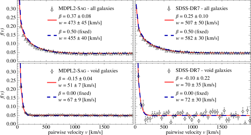
Figure 6: Measured and fitted pairwise velocity distributions. Upper panels correspond to all galaxies for MDPL2-Sag (left) and SDSS-DR7 (right). Bottom panels show the results for void galaxies for MDPL2-Sag (left) and SDSS-DR7 (right). The measured $f(v)$ is represented by triangles (all galaxies sample) and diamonds (void galaxies sample). Two model fits are shown: varying both $\beta$ and $w$ parameters in solid red lines and fixing $\beta$ to a fiducial value and varying only $w$ in dashed blue lines (see text for details). The values of the parameters $\beta$ and $w$ are shown in the respective key figures. Errorbars in measured points where estimated via the Jackknife resamplings of $\xi(\sigma,\pi)$.

	MDPL2-Sag	MDPL2-Sag	SDSS-DR7	SDSS-DR7
	all galaxies	void galaxies	all galaxies	void galaxies
$w$ [km/s]	$473\pm 45$	$50\pm 7$	$507\pm 50$	$70\pm 35$
$\beta$	$0.37\pm 0.05$	$-0.15\pm 0.04$	$0.25\pm 0.10$	$-0.10\pm 0.22$
$w$ [km/s]	$455\pm 40$	$67\pm 9$	$582\pm 30$	$72\pm 30$
$\beta$ (fixed)	$0.50$	$0.00$	$0.50$	$0.00$

Table 2: Values of the dynamical parameters $\beta$ and $w$, obtained by fitting the modeled pairwise velocity distribution to the measurements extracted from $\xi(\sigma,\pi)$. The first two rows corresponds to fitting both $\beta$ and $w$, meanwhile in the second two rows are the results obtained by fitting only $w$ with a fixed $\beta$ value (see text for details).

To provide the model fits, both $\beta$ and $w$ are taken as free parameters, and adjusted to the measured $f(v)$ by minimizing

$$\chi^{2}=\sum_{i=1}^{N}\left(\frac{f_{\rm data}(v_{i})-f_{\rm model}(v_{i})}{\epsilon_{i}}\right)^{2},$$ (16)

where $\epsilon_{i}$ are the data uncertainties and $N$ is the number of velocity bins. The values of $f_{\rm model}(v_{i})$ are also derived from the modeled $\xi(\sigma,\pi)$ via Eq. (8).

The results are given in Tab. 2, where it can be noticed the suitable agreement between MDPL2-Sag and SDSS-DR7 determinations of the $w$ and $\beta$ parameters. Quoted errors in the table correspond to estimates derived by the dispersion of the fitting parameters in realizations of $f(v)$ data including individual uncertainties of each velocity bin.

The resulting $f(v)$ distributions and the corresponding fits are shown in Fig. 6. The measured pairwise velocity distributions for all galaxies are plotted with triangles in the upper panels for MDPL2-Sag (left) and for SDSS-DR7 (right). The modeled $f(v)$ are shown with the grey solid curve. For void galaxies, we show measured and modeled $f(v)$ in the bottom panels, MDPL2-Sag at left and SDSS-DR7 at right. Measurements are shown with diamonds, and with the red solid and blue dashed lines the model fits. In all cases, the parameter values for $\beta$ and $w$ are shown in the key figures.

It can be seen in this figure the different shapes of $f(v)$ for all galaxies and void galaxies, reflecting the smaller redshift distortions observed in $\xi(s)$ for galaxies within voids (Sec. 3). These differences, observed in both the observations and in the simulated galaxies, is quantified by the fitting parameter values $w$ presented in Tab. 2. While for all galaxies we obtain a value $w\sim 500{\rm~{}km/s}$, for void galaxies the pairwise velocity dispersions range only between $w\sim 50-70{\rm~{}km/s}$, roughly one order of magnitude smaller.

We stress the fact that this method is not particularly sensible to obtain the $\beta$ parameter accurately from the derived $f(v)$ distributions, as discussed by Loveday et al. (2018). Furthermore, besides the best fitting pair of values $\beta$ and $w$, we have also tested the resulting velocity dispersions derived by fixing the $\beta$ parameter with two fiducial values: for galaxies in voids $\beta=0.00$ (assuming completely empty regions), and for all galaxies $\beta=0.50$ (corresponding to unbiased tracers in a $\Omega_{\rm m}=0.307$ model). It should be remarked that regardless the use of either best fitting parameters $\beta$ or fixed fiducial values, the derived pairwise velocity dispersion $w$ are in agreement within uncertainties. This can be appreciated by inspection to Fig. 6, where either varying or fixed $\beta$ values in the model provide suitable fitting curves to the derived $f(v)$.

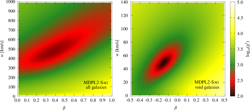
Figure 7: Maps of $\log_{10}(\chi^{2})$ resulting from the fitting procedure, described in Sec. 4.3 to determine $\beta$ and $w$ for the case of all galaxies (left) and void galaxies (right) in the MDPL2-Sag catalogue.

The $\beta$ and $w$ degeneracy in the model can be appreciated in Fig. 7, where we show the maps of $\log_{10}(\chi^{2})$ resulting from the fitting procedure to determine these parameters for the case of all galaxies (left) and void galaxies (right) in the MDPL2-Sag catalogue. In this figure it can also be seen the large range of allowed $\beta$ values, which implies very different cosmological and astrophysical scenarios ($\Omega_{\rm m}$ and $b$), whilst $w$ values are better constrained. Nevertheless, this approach is sufficient for our purpose to quantify with a simple modeling the dynamical behavior difference of galaxies in voids with respect to the general population.

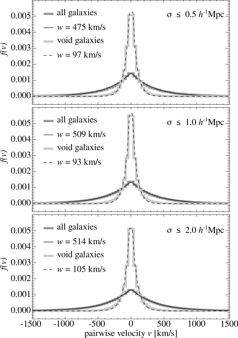
Figure 8: Pairwise velocity distributions measured in MDPL2-Sag catalogue. From top to bottom, the panels correspond to measurements of the line-of-sight relative velocity distributions for galaxy pairs in projected separations $\sigma\leq 0.5,~{}1.0~{}{\rm and}~{}2.0h^{-1}{\rm Mpc}$, respectively, as indicated in the top right legend of each panel. The distribution for all galaxies (void galaxies) are shown in dark (light) grey solid lines. In solid and dashed thin black lines are the exponential model fitted to each data sample.

We have also measured directly the $f(v)$ distributions for MDPL-Sag galaxies. These measures correspond to the line-of-sight relative velocity distributions for galaxy pairs in projected separations up to $0.5$, $1.0$ and $2.0h^{-1}{\rm Mpc}$, and including all pairs along the line-of-sight direction up to $20h^{-1}{\rm Mpc}$. The results are shown in Fig. 8 where, from top to bottom, we show the pairwise velocity distributions measured for all galaxies (dark-grey thick line) and void galaxies (light-grey thick lines) for $\sigma~{}\leq~{}0.5,~{}1.0~{}{\rm and}~{}2.0h^{-1}{\rm Mpc}$, respectively. The thin black lines correspond to exponential models given by Eq. (15) fitted to the distribution of all galaxies (solid lines) and void galaxies (dashed lines). The resulting fitting parameters $w$ given in the key figures are $w\sim 500{\rm~{}km/s}$ for all galaxies and $w\sim 100{\rm~{}km/s}$ for void galaxies, which compare suitably to those obtained by the methods derived previously in this Section.

5 Dependence of void internal structure on void environment

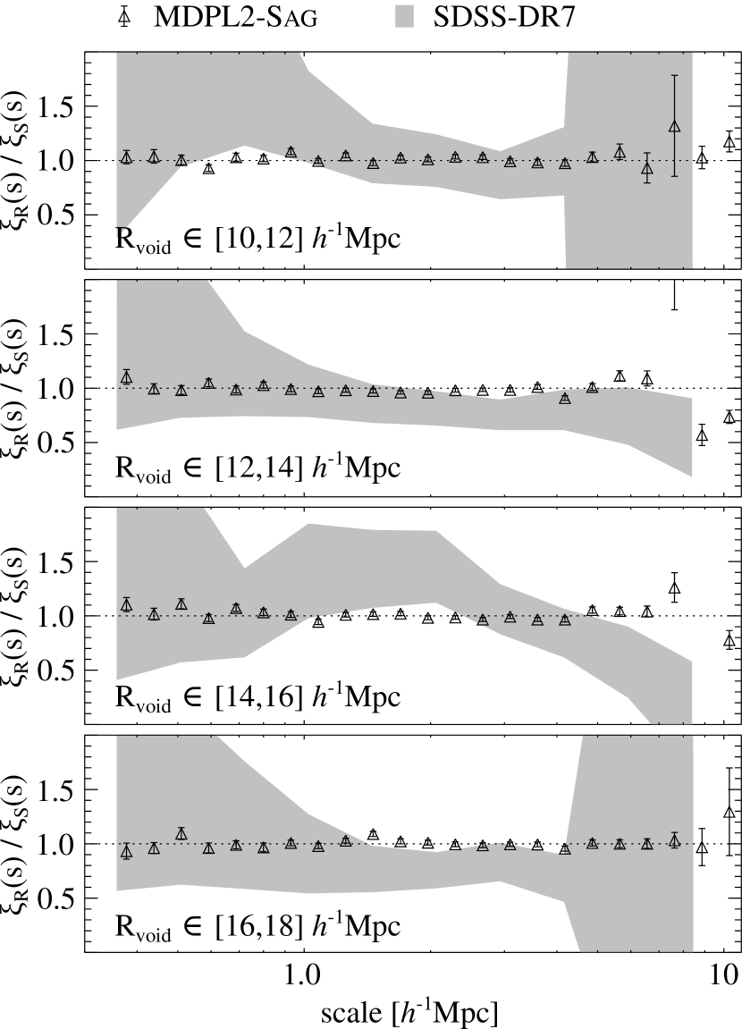
Figure 9: Ratio between the galaxy-galaxy redsfhit-space correlation functions inside R-type voids, $\xi_{\rm R}(s)$, and inside S-type voids, $\xi_{\rm S}(s)$. The panels correspond to different void radii interval, as indicated in the bottom left legends. In all cases, results for MDPL2-Sag are shown in black triangles and the results for SDSS-DR7 in grey areas.

Here we explore the possible dependence of spatial correlations and dynamics of galaxies within cosmic voids on their large-scale environment. A useful characterization of the void environment is given by the overdensity within 2 and 3 void radii (Ceccarelli et al., 2013; Paz et al., 2013; Ruiz et al., 2015), which corresponds to the void-in-void and void-in-cloud early classification by Sheth & van de Weygaert (2004). We remark that in spite of their different external environment, both types of voids are defined with the same constrains in terms of internal underdensity. R-type voids have underdense surroundings implying a continuously rising density profile even beyond $R_{\rm void}$, and so their future evolution is dominated by expansion. On the other hand, S-type voids are surrounding by shell-like structures which generates a collapse forecast of the void itself. We argue that by examining the properties of voids internal structure as measured by galaxy correlations, in both simulations and the observations, can provide further consistency tests of structure formation in the $\Lambda$CDM scenario.

In Fig. 9 we show the resulting ratio between the redshift-space correlation function of void galaxies inside R-type voids, $\xi_{\rm R}(s)$, and inside S-type voids, $\xi_{\rm S}(s)$. The black triangles correspond to MDPL2-Sag galaxies and the shaded regions to the SDSS-DR7 galaxies. The different panels correspond to different ranges of void radii as indicated in the key figures. Remarkably, it can be seen that the internal structure of voids, as measured by the correlation function, is unaffected by the external void environment irrespective of void radii. The large uncertainties associated to SDSS-DR7 measurements (given by the shaded areas) are due to the low number statistics of voids and galaxy pairs when the complete sample is divided both into radii ranges and void types. We notice however, that within the large uncertainties, the results are consistent with the lack of environmental dependence found in MDPL2-Sag.

6 Summary and conclusions

We have analysed the internal structure of cosmic voids as traced by faint galaxies using the two-point galaxy-galaxy correlation function. The results are compared to the global behaviour of galaxies with similar luminosities whose distribution and dynamics are dominated by those galaxies in large groups and clusters.

We apply our analysis to a sample of SDSS-DR7 galaxies, and tested our results with the semi-analytic catalogue MDPL2-Sag, obtaining a general suitable agreement with the observations.

For galaxies in voids, we obtain a similar shape for redshift-space and real-space correlation functions except for a nearly constant normalization factor which indicates small departures due to peculiar velocities of growing structure in voids. We find that correlations are remarkably linear in voids as compared with the general population which exhibit large departures due to the velocity dispersions of galaxies in clusters, absent in cosmic voids.

We have also computed the 2D correlation function $\xi(\sigma,\pi)$, where the large redshift-space distortions due to galaxy velocity dispersion in virialized systems is clearly absent for galaxies within voids compared to the global population.

From $\xi(\sigma,\pi)$, we infer the pairwise velocity distributions $f(v)$ of galaxies in cosmic voids and elsewhere for MDPL2-Sag and SDSS-DR7. For both observations and simulations, we find these distributions consistent with an exponential model with a pairwise velocity dispersion $w\sim 50-70{\rm~{}km/s}$, a figure significantly smaller than the derived global values of $w\sim 500{\rm~{}km/s}$. We recall the consistency of model and observational determinations which provide further support to the standard $\Lambda$CDM scenario of structure formation in a less explored regime of low-luminosity galaxies residing in global underdense regions.

For MDPL2-Sag galaxies, in addition to the derivation of $f(v)$ from $\xi(\sigma,\pi)$, we have computed directly for three different ranges of projected distance $\sigma\leq 0.5,~{}1.0,~{}{\rm and}~{}2.0h^{-1}{\rm Mpc}$. We find that in all cases the pairwise velocity distribution can be modeled by exponential functions with best fitting velocity dispersion parameters $w\sim 500{\rm~{}km/s}$ for all galaxies and $w\sim 100{\rm~{}km/s}$ for void galaxies, entirely consistent with the previous analysis.

Finally, we have tested the potential influence of the large-scale structure surrounding cosmic voids on the clustering of galaxies inside voids. We have compared the resulting $\xi(s)$ for galaxies in void-in-void (R-type voids) and void-in-cloud (S-type voids) (Sheth & van de Weygaert, 2004; Ceccarelli et al., 2013), for several void radius intervals, finding the same clustering amplitude of faint galaxies independent of the void environment. Namely, we find no influence of the surrounding structure beyond $R_{\rm void}$ on the internal void structure as traced by faint galaxies.

Our results show the potentiality of exploring the structure of cosmic voids through the distribution of faint galaxies. These void galaxies are not largely affected by strong non-linearities nor by gas dynamical effects, and their distribution is not influenced by the large-scale environment of voids. For these reasons, we argue that galaxies in voids may provide suitable samples to analyse possible subtle differences between the observations and current models of structure formation. These analysis may be extended in upcoming future galaxy surveys which can provide large datasets capable of extending our understanding of the spatial distribution and the dynamics of luminous and dark matter.

References

- Abazajian et al. (2009) Abazajian K. N., et al., 2009, ApJS, 182, 543
- Alpaslan et al. (2014) Alpaslan M., et al., 2014, MNRAS, 440, L106
- Aragon-Calvo & Szalay (2013) Aragon-Calvo M. A., Szalay A. S., 2013, MNRAS, 428, 3409
- Behroozi et al. (2013a) Behroozi P. S., Wechsler R. H., Wu H.-Y., 2013a, ApJ, 762, 109
- Behroozi et al. (2013b) Behroozi P. S., Wechsler R. H., Wu H.-Y., Busha M. T., Klypin A. A., Primack J. R., 2013b, ApJ, 763, 18
- Benson (2012) Benson A. J., 2012, New Astron., 17, 175
- Cautun et al. (2018) Cautun M., Paillas E., Cai Y.-C., Bose S., Armijo J., Li B., Padilla N., 2018, MNRAS, 476, 3195
- Ceccarelli et al. (2006) Ceccarelli L., Padilla N. D., Valotto C., Lambas D. G., 2006, MNRAS, 373, 1440
- Ceccarelli et al. (2008) Ceccarelli L., Padilla N., Lambas D. G., 2008, MNRAS, 390, L9
- Ceccarelli et al. (2013) Ceccarelli L., Paz D., Lares M., Padilla N., Lambas D. G., 2013, MNRAS, 434, 1435
- Colberg et al. (2008) Colberg J. M., et al., 2008, MNRAS, 387, 933
- Cole (2011) Cole S., 2011, MNRAS, 416, 739
- Cora et al. (2018) Cora S. A., et al., 2018, MNRAS, 479, 2
- Croton et al. (2016) Croton D. J., et al., 2016, ApJS, 222, 22
- Davis & Peebles (1983) Davis M., Peebles P. J. E., 1983, ApJ, 267, 465
- Diaferio & Geller (1996) Diaferio A., Geller M. J., 1996, ApJ, 467, 19
- Efron (1982) Efron B., 1982, The Jackknife, the bootstrap and other resampling plans. No. 38 in Regional Conference Series in applied mathematics, Society for Industrial and applied mathematics, Philadelphia, Pa.
- Górski et al. (2005) Górski K. M., Hivon E., Banday A. J., Wandelt B. D., Hansen F. K., Reinecke M., Bartelmann M., 2005, ApJ, 622, 759
- Gottlöber et al. (2003) Gottlöber S., Łokas E. L., Klypin A., Hoffman Y., 2003, MNRAS, 344, 715
- Hamilton (1992) Hamilton A. J. S., 1992, ApJ, 385, L5
- Hawkins et al. (2003) Hawkins E., et al., 2003, MNRAS, 346, 78
- Hoyle et al. (2005) Hoyle F., Rojas R. R., Vogeley M. S., Brinkmann J., 2005, ApJ, 620, 618
- Hoyle et al. (2012) Hoyle F., Vogeley M. S., Pan D., 2012, MNRAS, 426, 3041
- Kaiser (1987) Kaiser N., 1987, MNRAS, 227, 1
- Klypin et al. (2016) Klypin A., Yepes G., Gottlöber S., Prada F., Heß S., 2016, MNRAS, 457, 4340
- Knebe et al. (2015) Knebe A., et al., 2015, MNRAS, 451, 4029
- Knebe et al. (2018) Knebe A., et al., 2018, MNRAS, 474, 5206
- Lindner et al. (1996) Lindner U., et al., 1996, A&A, 314, 1
- Loveday et al. (2018) Loveday J., et al., 2018, MNRAS, 474, 3435
- Onions et al. (2012) Onions J., et al., 2012, MNRAS, 423, 1200
- Padilla et al. (2005) Padilla N. D., Ceccarelli L., Lambas D. G., 2005, MNRAS, 363, 977
- Patiri et al. (2006) Patiri S. G., Prada F., Holtzman J., Klypin A., Betancort-Rijo J., 2006, MNRAS, 372, 1710
- Paz et al. (2013) Paz D., Lares M., Ceccarelli L., Padilla N., Lambas D. G., 2013, MNRAS, 436, 3480
- Peebles (1980) Peebles P. J. E., 1980, The large-scale structure of the universe, Princeton University Press
- Planck Collaboration et al. (2014) Planck Collaboration et al., 2014, A&A, 571, A16
- Planck Collaboration et al. (2016) Planck Collaboration et al., 2016, A&A, 594, A13
- Pujol et al. (2017) Pujol A., et al., 2017, MNRAS, 469, 749
- Riebe et al. (2013) Riebe K., et al., 2013, Astronomische Nachrichten, 334, 691
- Rojas et al. (2004) Rojas R. R., Vogeley M. S., Hoyle F., Brinkmann J., 2004, ApJ, 617, 50
- Rojas et al. (2005) Rojas R. R., Vogeley M. S., Hoyle F., Brinkmann J., 2005, ApJ, 624, 571
- Ruiz et al. (2015) Ruiz A. N., Paz D. J., Lares M., Luparello H. E., Ceccarelli L., Lambas D. G., 2015, MNRAS, 448, 1471
- Saunders et al. (1992) Saunders W., Rowan-Robinson M., Lawrence A., 1992, MNRAS, 258, 134
- Sheth (1996) Sheth R. K., 1996, MNRAS, 279, 1310
- Sheth & van de Weygaert (2004) Sheth R. K., van de Weygaert R., 2004, MNRAS, 350, 517
- Strauss et al. (2002) Strauss M. A., et al., 2002, AJ, 124, 1810
- Tavasoli et al. (2015) Tavasoli S., Rahmani H., Khosroshahi H. G., Vasei K., Lehnert M. D., 2015, ApJ, 803, L13
- Tomita (2000) Tomita K., 2000, ApJ, 529, 38
- Voronoi (1908) Voronoi G., 1908, J. Reine Angew. Math., 1908 (133), 97
- York et al. (2000) York D. G., et al., 2000, AJ, 120, 1579