A predictive safety filter for learning-based control of constrained nonlinear dynamical systems

Abstract

The transfer of reinforcement learning (RL) techniques into real-world applications is challenged by safety requirements in the presence of physical limitations. Most RL methods, in particular the most popular algorithms, do not support explicit consideration of state and input constraints. In this paper, we address this problem for nonlinear systems with continuous state and input spaces by introducing a predictive safety filter, which is able to turn a constrained dynamical system into an unconstrained safe system and to which any RL algorithm can be applied ‘out-of-the-box’. The predictive safety filter receives the proposed control input and decides, based on the current system state, if it can be safely applied to the real system, or if it has to be modified otherwise. Safety is thereby established by a continuously updated safety policy, which is based on a model predictive control formulation using a data-driven system model and considering state and input dependent uncertainties.

AND FUNCTION

,

1 Introduction

Reinforcement learning (RL) has demonstrated its success in solving complex and high-dimensional control tasks, see for example Levine et al. (2016). These results motivate a more widespread transfer to real-world applications to enable automated design of high performance controllers with little need for expert knowledge. In physical systems, such as mechanical, thermal, biological, or chemical systems, physical limitations naturally arise as constraints, such as limited torque in the case of a robot arm or a limited power supply in building control. In addition to physical constraints, many relevant applications in industry require satisfaction of safety specifications, preventing, e.g., an autonomous car or aircraft from crashing, which can typically be formulated in terms of constraints on the system state. The simultaneous satisfaction of safety constraints under physical limitations during RL constitutes one of the main open problems in AI safety as discussed e.g. in Amodei et al. (2016, Section 3).

Significant progress in the safe operation of constrained systems has been made through model predictive control techniques, which provide rigorous constraint satisfaction, see, e.g., Mayne (2014). While model-based RL techniques such as Kamthe and Deisenroth (2017) are conceptually closely related to model predictive control, so far relatively few methods have considered safety guarantees. Learning-based model predictive control aims to combine the benefits of both fields, see for example Hewing et al. (2020) for an overview. In addition to the fact that designing such algorithms with rigorous safety guarantees is rather challenging, often conservative, and requires a considerable amount of expert knowledge, the approach is inherently restricted to a model-based control policy. More precisely, at each time step, a finite-horizon optimal control problem is solved in a receding horizon fashion in order to approximate a potentially infinite horizon optimal control policy.

Concept: We propose a model predictive control (MPC) variant as a predictive safety filter (PSF), that can turn highly nonlinear and safety-critical dynamical systems into inherently safe systems, and to which any RL algorithm without safety certificates can be applied ‘out-of-the-box’, see also Figure 1. Compared with a standard use of MPC, the PSF verifies if the input proposed by the RL algorithm is safe, otherwise it is entitled to modify the input as little as necessary to maintain safe operation at all future times. This means that the PSF only needs to keep the system safe instead of controlling it well with respect to a certain objective (e.g. comfort or economic criteria). The problem of finding a safety filter is therefore in general less complex than finding a desired optimal policy with respect to some objective and subject to constraints, motivating the combination of a predictive safety filter with an RL algorithm to safely optimize performance.

Differently to recently proposed related concepts presented in Gillula and Tomlin (2011); Wabersich and Zeilinger (2018a); Ames et al. (2019), we use the notion of a safe system in Figure 1, as similarly introduced in Wieland and Allgöwer (2007) within the context of safety barrier functions. The concept emphasizes the possibility that any RL algorithm that would have been used to control the original system can be applied to the safe system instead, yielding a certified safe RL application. The predictive safety filter provides safety at a desired level of probability, modularity in terms of the employed RL controller, and minimal intervention by filtering RL input signals only if we cannot guarantee safety at the specified probability level, similar to Fisac et al. (2019).

Figure 1: Concept of predictive safety filter: Based on the current state $x(k)$, a learning-based algorithm provides a control input $u_{\mathcal{L}}(k)=\pi_{\mathcal{L}}(k,x(k))\in\mathbb{R}^{m}$, which is processed by the safety filter $u(k)=\pi_{\mathcal{S}}(k,x(k),u_{\mathcal{L}}(k))$ and applied to the real system.

Contributions: Based on a probabilistic model of the system dynamics, which is inferred from data, this paper presents a predictive safety filter that builds on concepts from MPC for constrained nonlinear systems, and thereby generalizes the safety certification method for linear systems proposed by Wabersich and Zeilinger (2018a). Safety of an RL input is thereby enforced in real-time by searching for a safe backup trajectory for the next time step towards a known set of safe states. If necessary, to ensure safety for all times in the future, the search process for a backup trajectory is allowed to modify (filter) the RL input. As MPC typically outperforms non-optimization based techniques, e.g. based on control Lyapunov functions or sliding-mode controllers by solving an approximate optimal control problem on-line, the proposed PSF provides similar advantages compared with methods utilizing, e.g., control barrier functions for safety (Ames et al., 2019). More precisely, the PSF formulation provides an implicit representation of the set of safe state and input pairs, approximating the largest set of admissible states and inputs using finite-horizon MPC techniques. At the same time, the implicit safe set representation enables favorable scalability properties compared to, e.g., Hamilton-Jacobi-Bellman safety frameworks (Fisac et al., 2019) by avoiding offline computations that scale exponentially with the number of state dimensions. Clearly, these advantages come at the price of solving an optimization problem online, for which highly efficient tools are, however, available (Domahidi et al., 2012).

The application to nonlinear and probabilistic system descriptions, obtained, e.g., through machine learning techniques, is enabled via a nonlinear predictive safety filter formulation that is robust in probability and supports state and input dependent uncertainty information. Robustness with respect to non-uniform model uncertainties is enabled by restricting predicted backup trajectories to confident subsets of the state and input space. The corresponding online optimization problem has similar computational complexity to nominal MPC problems, while being less conservative compared to other robust MPC approaches (Hewing et al., 2020, Section 3.1) that are often based on a uniform uncertainty bound. The proposed formulation leads to a theoretical analysis that rigorously relates parameters of the predictive safety filter and accuracy of its system model to safety in probability. Depending on the desired constraint satisfaction probability, this enables safe exploration beyond available data.

We illustrate the approach using a simulated pendulum swing-up task, in which only little initial data around the stable downward position is available and overshoots of the upward position are prohibited, imposing challenging safety constraints on the system. Scalability and practical implementation are demonstrated in a quadrotor simulation example, considering the task of learning to quickly approach a landing position for a full-scale model with 12 states and 4 inputs.

Discussion: While the focus of this paper is the certification of RL algorithms, the concept can also be used together with, e.g., human inputs. For example, in the case of autonomous driving, the safety filter could be used to ensure safety of either an RL-based controller or a human driver, and can be viewed as a driver assistance system that is able to overrule the student driver (or RL algorithm), if necessary for safety.

2 Related Work

Safe model-free reinforcement learning: There is a growing awareness of safety questions in the domain of artificial intelligence (Amodei et al., 2016), and several safe reinforcement learning techniques have been proposed, see e.g. Garcıa and Fernández (2015) for an overview. Achiam et al. (2017), e.g., provide safety in expectation based on a trust-region approach with respect to the policy gradient.

Most notions of safety considered in this line of research, e.g. one-step constraint satisfaction in expectation, tend to be less strict compared with the probabilistic safety requirements at all time steps in the future as considered in this paper. More importantly, since most techniques are policy-based, safety is coupled to a specific policy and therefore potentially also to a specific task, limiting generalization of the safety certificates.

Learning-based model predictive control: Originating from concepts in robust model predictive control (MPC), extensions of MPC schemes to safe learning-based methods have been proposed, see e.g. Hewing et al. (2020) for a review. In addition, various results have investigated combinations of MPC with learning-based online model identification techniques (Ostafew et al., 2016; Limon et al., 2017; Koller et al., 2018; Soloperto et al., 2018), also in an adaptive manner (Tanaskovic et al., 2013). In the context of robotics, similar concepts exist, which are often referred to as funneling, see e.g. Majumdar and Tedrake (2017) and references therein, as well as so called LQR-trees (Tedrake et al., 2010).

While some of these techniques have been demonstrated to work well in practice (Bouffard et al., 2012; Ostafew et al., 2016; Hewing et al., 2018), they typically either lack rigorous theoretical safety guarantees, tend to be overly conservative by relying on Lipschitz-based estimates in the prediction of the uncertain system evolution, or are restricted to a very specific system class.

Model-based policy certification through barrier functions and safety frameworks: Conceptually, the idea of safety architectures, as illustrated in Figure 1, was originally proposed by Seto et al. (1998), where a principled switching between a safety controller and basic/experimental controllers enables safe controller tuning online. Based on this concept, control theoretic frameworks have been developed (Prajna and Jadbabaic, 2004), related to control Lyapunov functions (Wieland and Allgöwer, 2007), and have also become known as control barrier functions, see Ames et al. (2019) for an overview. Recent developments also consider the combination with learning tasks through data-driven models (Ohnishi et al., 2019). While such frameworks inherit strong theoretical results from control Lyapunov function theory, they require the explicit availability of a control barrier function, which is difficult to compute in general. In particular, to the best of the authors’ knowledge, only approximate approaches exist using ellipsoidal or sum-of-squares computations (Wang et al., 2018) to design a safety barrier function with respect to given, e.g. polytopic, state and input constraints.

In the case of partially known system dynamics, the concept of a control barrier function can be combined with Bayesian model estimates from data that validate the resulting closed-loop system (Berkenkamp et al., 2016). The techniques share similar limitations with safe model-free RL methods, namely that they are tailored to a specific task. A task-independent learning-based safety framework has been introduced in Gillula and Tomlin (2011), which generalizes the concept of explicitly knowing a barrier function. It consists of a model-based safe set of system states and computes a corresponding safe control policy, which is entitled to override a potentially unsafe RL algorithm to ensure invariance with respect to the safe set of system states i.e. containment within the safe set at all times. This concept was further developed in several papers, providing principled methods to compute the safe set as well as the corresponding safe policy (Fisac et al., 2019; Wabersich and Zeilinger, 2018b), which build the foundation of the safety filter presented in this paper.

The aforementioned techniques related to both safety barrier functions and safety frameworks either suffer from limited scalability to higher dimensional and complex systems, or only provide principled design computations for specific constrained model classes, such as linear or polynomial models. While also building on the same high-level concept, this paper addresses these limitations by 1) considering a stochastic nonlinear system model belief, which is well-suited to learning-based control of highly nonlinear and unstable system dynamics, and 2) a unified MPC-inspired formulation for the safety policy (predictive safety filter), which avoids the explicit computation of a safety barrier function or a safe set.

In particular, compared to similar MPC-inspired safety mechanisms such as Wabersich and Zeilinger (2018a); Mannucci et al. (2018); Li and Bastani (2019), we consider nonlinear system models with stochastic parameter uncertainties and provide a predictive safety filter formulation that is capable of leveraging the resulting state and input dependent uncertainty estimates to reduce conservatism.

3 Problem Statement

Notation: The set of integers in the interval $[a,b]\subset\mathbb{R}$ is $\mathcal{I}_{[a,b]}$, and the set of integers in the interval $[a,\infty)\subset\mathbb{R}$ is $\mathcal{I}_{\geq a}$. The $i$-th row and $i$-th column of a matrix $A\in\mathbb{R}^{n\times m}$ is denoted by $\mathrm{row}_{i}(A)$ and $\mathrm{col}_{i}(A)$. By $\mathbbm{1}_{n}$ we denote the vector of ones with length $n$. $\lhd$

Consider deterministic discrete-time systems of the form

$$x(k+1)=f(x(k),u(k);\theta_{\mathcal{R}}),~{}\forall k\in\mathcal{I}_{\geq 0},$$ (1)

with dynamics $f:\mathbb{X}\times\mathbb{U}\rightarrow\mathbb{R}^{n}$ parametrized by $\theta_{\mathcal{R}}\in\mathbb{R}^{p}$ and stochastic initial condition $x(0)=x_{\mathrm{init}}\in\mathbb{X}$ with known distribution $p(x_{\mathrm{init}})$. The system is subject to polyhedral state and input constraints $\mathbb{X}\coloneqq\{x\in\mathbb{R}^{n}|A_{x}x\leq\mathbbm{1}_{n_{x}}\}$ and $\mathbb{U}\coloneqq\{u\in\mathbb{R}^{m}|A_{u}u\leq\mathbbm{1}_{n_{u}}\}$, originating from physical limitations and safety requirements. We consider the case of unknown ‘real’ parameters $\theta_{\mathcal{R}}$, but assume the availability of a distribution

$$\theta\sim p(\theta)\text{ with mean }\mathbb{E}\left[\theta\right],$$ (2)

which can be estimated from data. The overall objective is to safely find a policy $\pi_{\mathcal{L}}:\mathcal{I}_{\geq 0}\times\mathbb{X}\rightarrow\mathbb{U}$ that either minimizes an episodic, finite-time or infinite horizon objective

$$J_{\bar{N}}(x(k))=\mathbb{E}\left[\sum_{i=k}^{\bar{N}}\ell\big{(}x(i),\pi_{\mathcal{L}}(i,x(i))\big{)}\right]$$ (3)

with $\bar{N}\in\mathbb{N}$, and stochastic stage cost $\ell(x,u)\coloneqq\bar{\ell}(x,u)+w_{\ell}$ consisting of a deterministic part $\bar{\ell}:\mathbb{X}\times\mathbb{U}\rightarrow\mathbb{R}$ and zero mean i.i.d. stochastic noise $w_{\ell}$. In order to prescribe a desired level of caution and desired conservatism in exploration, we consider safety in terms of constraint satisfaction at a desired probability level $p_{\mathcal{S}}>0$ as

$$\Pr\left(\forall k\in\mathcal{I}_{[0,\bar{N}]}:x(k)\in\mathbb{X},u(k)\in\mathbb{U}\right) \geq p_{\mathcal{S}}.$$ (4)

This paper addresses the problem of implementing a safety filter as shown in Figure 1, which ensures closed-loop safety according to (4). The filter enables application of any RL algorithm to the virtual input of the safe system, i.e. $u_{\mathcal{L}}(k)=\pi_{\mathcal{L}}(k,x(k))$, with the goal of minimizing the objective, while ensuring safety by selecting the input to the real system as $u(k)=\pi_{\mathcal{S}}(k,x(k),u_{\mathcal{L}}(k))$. In other words, the approach turns a safety-critical task into an unconstrained task with respect to the safe system dynamics $f_{\mathcal{S}}(k,x(k),u_{\mathcal{L}}(k))\coloneqq f(x(k),\pi_{\mathcal{S}}(k,x(k),u_{\mathcal{L}}(k)))$ such that any RL algorithm can be safely applied, see Figure 1. To further specify the desired properties of $\pi_{\mathcal{S}}$, consider the following definition of a safety certified learning-based control input.

Definition 3.1.

An input $u_{\mathcal{L}}(\bar{k})$ is certified as safe for system (1) at time step $\bar{k}$ and state $x(\bar{k})$ with respect to a safety filter $\pi_{\mathcal{S}}:\mathcal{I}_{\geq 0}\times\mathbb{X}\times\mathbb{U}\rightarrow\mathbb{U}$, if $\pi_{\mathcal{S}}(\bar{k},x(\bar{k}),u_{\mathcal{L}}(\bar{k}))=u_{\mathcal{L}}(\bar{k})$ and application of $u(k)=\pi_{\mathcal{S}}(k,x(k),u_{\mathcal{L}}(k))$ for $k\geq\bar{k}$ implies safety for all times according to (4).

Following this definition, the goal is to provide a safety filter $\pi_{\mathcal{S}}$ that restricts learning as little as possible by certifying a large set of learning inputs $u_{\mathcal{L}}(k)$ for a given state $x(k)$. If the learning input cannot be certified as safe, the safety filter provides an alternative safe input, i.e. $u(k)=\pi_{\mathcal{S}}(k,x(k),u_{\mathcal{L}}(k))\neq u_{\mathcal{L}}(k)$, where the filter aims at the smallest possible modification by, e.g., minimizing $\left\lVert{\pi_{\mathcal{S}}(k,x(k),u_{\mathcal{L}}(k))-u_{\mathcal{L}}(k)}\right\rVert_{2}$. The following section introduces the mechanisms of the proposed predictive safety filter, which builds on a predictive constrained control formulation, planning safe trajectories based on a probabilistic model belief to ensure safe system operation at all times according to (4).

Nominal Predictive Safety Filter

Nominal online problem:

$$\min_{\begin{subarray}{c}\{u_{i|k}\}\end{subarray}}~{} \left\lVert{u_{\mathcal{L}}-u_{0|k}}\right\rVert$$ (5a)

s.t. $$~{}\forall i\in\mathcal{I}_{[0,N-1]}:$$

$$x_{i+1|k}=f(x_{i|k},u_{i|k};\bar{\theta}),~{}$$ (5b)

$$x_{i|k}\in\mathbb{X},~{}$$ (5c)

$$u_{i|k}\in\mathbb{U},~{}$$ (5d)

$$(x_{i|k},u_{i|k})\in\mathbb{Z}_{c},~{}$$ (5e)

$$x_{N|k}\in\mathcal{S}^{t},$$ (5f)

$$x_{0|k}=x(k).$$ (5g)

Algorithm 1 (Nominal PSF):

function $\pi_{\mathcal{N}\mathcal{S}}$($k,x(k),u_{\mathcal{L}}(k)$)

     if (5) is feasible for horizon $N$ then

         Define $\bar{k}\coloneqq k$

         return $u^{*}_{0|k,N}$

     else if $k<N+\bar{k}$ then

         Solve (5) for horizon $N-(k-\bar{k})$

         return $u^{*}_{0|k,N-(k-\bar{k})}$

     else

         return $\pi_{\mathcal{S}}^{t}(x(k))$

     end if

end function

Illustration of nominal PSF:

  Predictive Safety Filter Online problem: $\displaystyle\min_{\begin{subarray}{c}\{{v}_{i|k}\}\end{subarray}}~{}$ $\displaystyle\left\lVert{u_{\mathcal{L}}-{v}_{0|k}}\right\rVert$ (6a) s.t. $\displaystyle~{}\forall i\in\mathcal{I}_{[0,N-1]}:$ $\displaystyle\mu_{i+1|k}=f(\mu_{i|k},{v}_{i|k};\bar{\theta}),~{}$ (6b) $\displaystyle\mu_{i|k}\in\bar{\mathbb{X}}_{i},~{}$ (6c) $\displaystyle{v}_{i|k}\in\bar{\mathbb{U}}_{i},~{}$ (6d) $\displaystyle\mathcal{E}_{p_{\mathcal{S}}}(\mu_{i|k},{v}_{i|k})\subseteq\bar{\mathcal{E}}_{i}^{\gamma},~{}$ (6e) $\displaystyle\mu_{N|k}\in\bar{\mathcal{S}}^{t}_{N},$ (6f) $\displaystyle\mu_{0|k}=x(k).$ (6g) Algorithm 2 (PSF): function $\pi_{\mathcal{S}}$($k,x(k),u_{\mathcal{L}}(k)$)      if (6) is feasible for horizon $N$ then          Define $\bar{k}\coloneqq k$          return ${v}^{*}_{0|k,N}$      else if $k<N+\bar{k}$ then          Solve (6) for horizon $N-(k-\bar{k})$          return ${v}^{*}_{0|N-(k-\bar{k})}$      else          return $\pi_{\mathcal{S}}^{t}(x(k))$      end if end function Illustration of PSF under uncertainty:

Figure 2: The basic idea of the predictive safety filter explained using a nominal, simplified version in the left column and the final method on the right. The illustrations show the system state at time $k$ with safe backup plan for a shorter horizon obtained from the solution at time $k-1$, depicted in brown, and areas with poor model quality in red. An arbitrary learning input $u_{\mathcal{L}}$ is certified if a feasible solution towards the terminal safe set $\mathcal{S}^{t}$ can be found, as shown in green. If this new backup solution cannot be found and the planning problem (5)/(6) is infeasible, the system can be driven to the safe set $\mathcal{S}^{t}$ along the brown previously computed trajectory. Left (NPSF): By assuming perfect system knowledge, the computed backup plans correspond exactly to the true state dynamics and constraints are guaranteed to be satisfied using the nominal backup trajectory. Right (PSF): Backup plans are computed w.r.t. the nominal expected state $\mu$. The true state trajectory lies within a growing tube around the nominal state with probability $p_{\mathcal{S}}$, which needs to be considered using tightened constraints according to (9).

4 Predictive safety filter

We first develop an intuitive understanding of the predictive safety filter by considering a simplified setting and assuming perfect model knowledge in Section 4.1, which is then extended in Section 4.2 to an uncertain model (1), (2) inferred from data, for which rigorous proofs are provided. As it will be shown, the presented method establishes safety by relying on controllability of (1) along system trajectories, in combination with an efficient mechanism enforcing the system to carefully enter uncertain areas within the state and input space.

4.1 Nominal (simplified) predictive safety filter

Consider the simplified situation where the real system dynamics (1) are perfectly known for some subset of the state and input space, as specified in the following.

Assumption 4.1.

There exists a set $\mathbb{Z}_{c}\subseteq\mathbb{X}\times\mathbb{U}$, such that for all $(x,u)\in\mathbb{Z}_{c}$ and some $\bar{\theta}\in\mathbb{R}^{p}$ it holds that $f(x,u;\bar{\theta})=f(x,u;\theta_{\mathcal{R}})$.

Similarly to Wabersich and Zeilinger (2018a), we propose a predictive safety filter that is not pre-computed, but defined via an optimization problem and computed on-the-fly. The main working mechanism is the construction of safe backup plans that, if applied, would keep the system provably safe in the future, see Figure 2 (left) for an illustration. The backup plans are defined via (5), where $\{x_{i|k,N}\}$ denote the planned states computed at the current time step $k$ and predicted $i$ time steps into the future with planning horizon $N$ using the corresponding input sequence $\{u_{i|k,N}\}$. One of the key challenges in computing the backup plans is to deal with the fact that a good model is not known in unexplored regions of the state-space, i.e. $\mathbb{X}\setminus\mathbb{Z}_{c}$, shown as red (unconfident model) sets in Figure 2. In the nominal setting, we simply address this problem by enforcing the system to strictly stay within the confident model subset $\mathbb{Z}_{c}$ via (5e). One of the main problems addressed in the next section will be to relax this constraint to enable cautious exploration of such unconfident subsets. The purpose of the remaining constraints in (5) is to construct backup plans that lead the system within state and input constraints $\mathbb{X}$ and $\mathbb{U}$ (5c), (5d) into a safe terminal set $\mathcal{S}^{t}$ in $N$ steps (5f).

The objective of constructing the backup plans in (5) is to minimize the deviation between the first element of the input sequence $u_{0|k,N}$ and the input $u_{\mathcal{L}}(k)$ requested by the RL algorithm, such that $u_{0|k,N}=u_{\mathcal{L}}(k)$ if $u_{\mathcal{L}}(k)$ is safe. Conceptually, this mechanism is similar to QP-based barrier function methods (Ames et al., 2017), where the input is adjusted to remain inside an explicitly known invariant set, with the key difference that here the safe set is implicitly defined. The resulting nominal predictive safety filter is then given by $\pi_{\mathcal{N}\mathcal{S}}(k,x(k),u_{\mathcal{L}}(k))=u^{*}_{0|k,N}$, with $u^{*}_{0|k,N}$ being the optimal first control input obtained from (5) based on a prediction horizon of length $N$. To ensure constraint satisfaction beyond the planning horizon, (5) utilizes a mechanism common in predictive control (see e.g. Chen and Allgöwer (1998)), by requiring the last state of the sequence $\{x_{N|k,N}\}$ to lie in a safe terminal set of system states $\mathcal{S}^{t}$, for which a locally valid safety filter $\pi_{\mathcal{S}}^{t}$ is known.

Assumption 4.2.

There exists a terminal safe set $\mathcal{S}^{t}\coloneqq\{x\in\mathbb{R}^{n}|a_{\mathcal{S}}(x)\leq\mathbbm{1}_{n_{\mathcal{S}}}\}\subseteq\mathbb{X}$, with $a_{\mathcal{S}}$ Lipschitz continuous with Lipschitz constant $L_{\mathcal{S}}$, and a corresponding terminal safety filter $\pi_{\mathcal{S}}^{t}:\mathcal{I}_{\geq 0}\times\mathbb{X}\times\mathbb{U}\rightarrow\mathbb{U}$, such that if $x(\bar{k})\in\mathcal{S}^{t}$, then application of $u(k)=\pi_{\mathcal{S}}^{t}(k,x(k),u_{\mathcal{L}}(k))$ implies that $x(k)\in\mathbb{X}$ and $u(k)\in\mathbb{U}$ for all $k>\bar{k}$.

A terminal safe set $\mathcal{S}^{t}$ and the corresponding controller $\pi_{\mathcal{S}}^{t}$ can be chosen, e.g., as a classical terminal set for nonlinear (robust) MPC (Chen and Allgöwer, 1998), regions around stable steady-states of system (1), or using expert system knowledge as is demonstrated in Section 5.

Based on problem (5), the predictive safety filter $\pi_{\mathcal{S}}$ is defined by Algorithm 1 (Figure 2, left). At every time step, we attempt to solve optimization problem (5). If problem (5) is feasible at time $k$, safety, i.e., $x(k)\in\mathbb{X}$, $u(k)\in\mathbb{U}$, directly follows from (5c), (5d). Due to the generality of the terminal safe set, however, problem (5) may become infeasible for some state $x(k)$, even after being feasible at the previous time step $x(k-1)$. Algorithm 1 implements a shrinking horizon mechanism similar to Thomas et al. (1994); Grune and Palma (2014) to also provide a feasible safe trajectory and input sequence towards the terminal safe set for this case, as detailed in the following:

Assume that (5) was feasible at time $k-1$ with corresponding optimal input sequence $\{u^{*}_{i|k-1,N}\}$. Application of $u(k-1)=u^{*}_{0|k-1,N}$ results in a safe state $x(k)$ as depicted in Figure 2 (left), because $(x(k-1),u(k-1))\in\mathbb{Z}_{c}$ by (5e) and therefore $x(k)=f(x(k-1),u(k-1);\bar{\theta})\in\mathbb{X}$ by (5c). At the next time step $k$, if (5) is not feasible, we can still solve (5) with a reduced planning horizon $N-1$. This can be easily verified by noting that $u_{i|k}=u^{*}_{i+1|k-1}$ for $i\in\mathcal{I}_{[0,N-2]}$, i.e. the tail of the previously computed feasible trajectory from time step $k-1$, is a feasible solution as depicted by the brown trajectory in Figure 2 (left). Feasibility of (5) for a reduced horizon again directly provides $x(k)\in\mathbb{X}$, $u(k)\in\mathbb{U}$.

The same holds true in the case that $j<N$ steps were consecutively infeasible for planning horizon $N$, i.e. (5) will then be feasible with horizon $N-j$ until we reach the safe terminal set. This shortening of the horizon is implemented in lines 6-7 of Algorithm 1. If the horizon length reaches $0$, the state is in the terminal set and $\pi_{\mathcal{S}}^{t}$ can be applied to ensure $x(k)\in\mathbb{X}$, $u(k)\in\mathbb{U}$ (line 9). Note again that if (5) is feasible at time $k$ (line 3-4), $u^{*}_{0|k,N}$ can be applied, which ideally results in $u_{\mathcal{L}}(k)$ (i.e. objective (5a) is zero) as shown in Figure 2 (left) together with the optimal backup plan in green. Algorithm 1 therefore ensures constraint satisfaction at all time steps, realizing a predictive safety filter in a receding horizon fashion with varying prediction length. The next section will extend the previously introduced basic concept of the predictive safety filter to consider a data-driven approximate system belief, represented by (1), (2), subject to probabilistic constraint satisfaction (4).

4.2 Predictive safety filter

A key goal of the safety filter is to support exploration beyond available data via the learning policy $\pi_{\mathcal{L}}(k)$, in which case Assumption 4.1 does not necessarily hold. While fast approximate computation of the backup trajectories can still be performed online using the mean estimate $\bar{\theta}$ of the parameter $\theta_{\mathcal{R}}$, we need to safely handle the resulting non-vanishing model error

$$e(k,\theta_{\mathcal{R}})\coloneqq f(x(k),u(k);\theta_{\mathcal{R}})-f(x(k),u(k);\bar{\theta}).$$ (7)

In the following, we first treat uncertainty via a uniform error bound to introduce the safety filter for uncertain systems, which is then extended to consider a less conservative bound and impose it as a constraint in the filter planning problem, in order to reduce conservatism.

Uniformly bounded model error: Assume that the model error with respect to the point estimate $\bar{\theta}$ can be bounded as

$$\Pr(e(k,\theta_{\mathcal{R}})\in\mathcal{E}\text{ for all~{}}k\in\mathcal{I}_{\geq 0})\geq p_{\mathcal{S}}$$ (8)

with $\mathcal{E}\coloneqq\{e\in\mathbb{R}^{n}|a_{\mathcal{E}}(e)\leq\mathbbm{1}_{n_{\mathcal{E}}}\}$ and $a_{\mathcal{E}}:\mathbb{R}^{n}\rightarrow\mathbb{R}^{n_{\mathcal{E}}}$ Lipschitz continuous and linearly bounded from below, i.e. constants $L_{a_{\mathcal{E}}}>0$ and $c_{\mathcal{E}}>0$ exist such that $c_{\mathcal{E}}\lVert{e}\rVert_{2}\leq\lVert{a_{\mathcal{E}}(e)}\rVert_{2}\leq L_{a_{\mathcal{E}}}\lVert{e}\rVert_{2}$, which implies compactness of $\mathcal{E}$. In this case, the filter can still compute backup plans using the point estimate $\bar{\theta}$, however, in contrast to the nominal case in Section 4.1, the constraints in (5) are modified such that prediction errors induced by (7) are compensated to ensure constraint satisfaction.

We denote the nominal (expected) system states as $\{\mu_{i|k}\}$, corresponding to the nominal input sequence $\{{v}_{i|k}\}$ according to $\mu_{i+1|k}=f(\mu_{i|k},{v}_{i|k};\bar{\theta})$. Due to the model error (7), we need to address the fact that potentially $x(k+1)\notin\mathbb{X}$, i.e. $A_{x}x(k+1)\nleq\mathbbm{1}_{n_{x}}$, when applying the nominal input ${v}_{0|k}$, even though the corresponding nominal predicted state satisfies ${\mu}^{*}_{1|k}\in\mathbb{X}$. A common strategy for achieving robustness in predictive control is to tighten the constraints by leveraging controllability along any possible predicted state sequence $\{\mu_{i|k}\}$ (Mayne, 2014). Intuitively speaking, controllability enables efficient compensation of deviations $x(i)-\mu_{i|k}$ via feedback control. More precisely, the possible deviations can be bounded by a decay constant, expressed by a parameter $\rho$, at which a controller can compensate disturbances of a certain magnitude, defined proportionally to a parameter $\epsilon$. Using these two measures, deviations from the planned nominal trajectory can be compensated via an iterative tightening of the constraints. This allows a flexible response to upcoming disturbances at the desired probability level $p_{\mathcal{S}}$ during consecutive time steps via replanning, thereby enabling overall constraint satisfaction. Following Köhler et al. (2018b), we tighten the constraints (5c), (5d), and (5f) in the computation of the backup plans as

$$\bar{\mathbb{X}}_{i} \coloneqq\{x\in\mathbb{R}^{n}|A_{x}x\leq(1-\epsilon_{i})\mathbbm{1}_{n_{x}}\},$$ (9a)

$$\bar{\mathbb{U}}_{i} \coloneqq\{u\in\mathbb{R}^{m}|A_{u}u\leq(1-\epsilon_{i})\mathbbm{1}_{n_{u}}\},$$ (9b)

$$\bar{\mathcal{S}}_{N}^{f} \coloneqq\{x\in\mathbb{R}^{n}|a_{\mathcal{S}}(x)\leq(1-\epsilon_{N})\mathbbm{1}_{n_{\mathcal{S}}}\},$$ (9c)

implementing a trade-off between compensation and magnitude of disturbances via the converging recursion

$$\begin{rcases*}\epsilon_{0}\coloneqq 0\\ \epsilon_{i+1}\coloneqq\epsilon_{i}+\sqrt{\rho}^{i}\epsilon\end{rcases*}\Rightarrow\epsilon_{i}=\epsilon\frac{1-\sqrt{\rho}^{i}}{1-\sqrt{\rho}},$$ (10)

with design parameter $\epsilon>0$ and parameter $\rho\in(0,1)$ that depends on system (1) as follows.

Assumption 4.3.

There exists a control policy $\pi:\mathbb{X}\times\mathbb{X}\times\mathbb{U}\rightarrow\mathbb{R}^{m}$, a function $V:\mathbb{X}\times\mathbb{X}\times\mathbb{U}\rightarrow\mathbb{R}_{\geq 0}$, which is continuous in its first argument and satisfies $V(x,x,v)=0$ for all $x\in\mathbb{X}$, $v\in\mathbb{U}$, and parameters $c_{l},c_{u},\delta,\pi_{\mathrm{max}}\in\mathbb{R}_{\geq 0}$, $\rho\in(0,1)$, such that for a given $\bar{\theta}\in\mathbb{R}^{q}$ the following properties hold for all $x,\mu\in\mathbb{X}$, $v,v^{+}\in\mathbb{U}$:

$$c_{l}\left\lVert{x-\mu}\right\rVert_{2}^{2}\leq V(x,\mu,v)\leq c_{u}\left\lVert{x-\mu}\right\rVert_{2}^{2}$$

and if in addition $$V(x,\mu,v)\leq\delta$$ then

$$\left\lVert{\pi(x,\mu,v)-v}\right\rVert_{2}\leq\pi_{\mathrm{max}}\left\lVert{x-\mu}\right\rVert_{2}$$

$$V\left(f(x,\pi(x,\mu,v);\bar{\theta}),f(\mu,v;\bar{\theta}),v^{+}\right)\leq\rho V(x,\mu,v).$$

Informally, Assumption 4.3 defines how well the uncertain system can be controlled in a neighborhood of predicted nominal backup plans $\{{\mu}^{*}_{i|k}\}$. Intuitively speaking, considering the task of tracking a reference trajectory as an optimal control problem with value function $V$ (using for example a linear quadratic regulator in the linear dynamics setting), parameter $\rho$ defines ‘how fast’ a reference can be reached, measured in terms of the contraction rate of the optimal tracking cost $V$. Interestingly, this translates into a system-theoretic requirement on system (1), or more precisely to local incremental stabilizability, which can be formally verified based on a system linearization, as discussed in Köhler et al. (2018a, Prop. 1). The condition can also be found in Appendix A.6 and provides explicit choices for $V$ and $\pi$. It is, however, important to note that the final algorithm only requires existence of the policy $\pi$ and the corresponding function $V$, rather than their explicit form.

These concepts lead to a robustified version of the nominal predictive safety filter defined in (6) and Algorithm 2 (Figure 2, right), where we omit (6e) in the case of uniformly bounded errors (8). Assumption 4.3 ties the model uncertainty (8) to the constraint tightening (9) to ensure the existence of a safe backup plan at all times and allows extension of the arguments for the nominal case to a probabilistic model belief. If (6) is feasible at time $k-1$ and the error bound $\mathcal{E}$ according to (8), i.e. $\max_{e\in\mathcal{E}}\left\lVert{e}\right\rVert_{2}$, is sufficiently small with respect to $\epsilon$ (see also Sections 4.3 for a detailed discussion) with probability $p_{\mathcal{S}}$, then at time $k$, the input sequence based on the plan computed at time step $k-1$

$${v}_{i|k}\coloneqq\pi(\mu_{i|k},{\mu}^{*}_{i+1|k-1,N},{v}^{*}_{i+1|k-1,N})$$ (11)

for $i\in\mathcal{I}_{[0,N-2]}$ with $\mu_{0|k}=x(k)$, $\pi$ according to Assumption 4.3, and $\mu_{i|k}$ according to (6b), provides a feasible solution to (6) with planning horizon $N-1$ (Algorithm 2, line 6) with probability $p_{\mathcal{S}}$. Again, the tracking policy $\pi$ is only used in order to show that a solution to (6) exists, but it is not needed for implementation of the approach. The same argument holds true for all $\bar{k}\in\mathcal{I}_{[k+1,k+N-1]}$ until the terminal set is reached (line 10), which allows us to establish safety at all times similarly to the nominal case. A formal proof will be given in the following for the more general case including a constraint on model confidence.

Planning in confident subspaces: To reduce conservatism introduced by uniformly overbounding the uncertainty in (8), a central novelty in the proposed safety filter is the ability to restrict planning to regions in the state and input space $\mathbb{Z}_{c}$ (see also Figure 2) where we are sufficiently confident about the system dynamics. More precisely, we restrict predictions to subspaces where the model error (7) is contained in a pre-specified, reduced allowable error set of the form

$$\mathcal{E}^{\gamma}\coloneqq\{e\in\mathbb{R}^{n}|a_{\mathcal{E}}(e)\leq\gamma\mathbbm{1}_{n_{\mathcal{E}}}\},\quad 0<\gamma\leq 1$$ (12)

with scaling factor $\gamma$, which allows easy adjustment of the maximum error magnitude due to the relation $e\in\mathcal{E}^{\gamma}\Rightarrow\lVert{e}\rVert_{2}\leq(\sqrt{n_{\mathcal{E}}}/c_{\mathcal{E}})\gamma$, see proof of Lemma A.4. A simple approach would be to compute the region $\mathbb{Z}_{c}$ offline and add it as an additional state and input constraint, as was similarly done for the case of linear dynamics with state dependent uncertainties by Soloperto et al. (2018). However, it is in general difficult to compute $\mathbb{Z}_{c}$ analytically and in addition, the set needs to be recomputed once the model belief (1), (2) is updated based on observed data. We therefore reformulate the requirement to stay inside $\mathbb{Z}_{c}$ as an implicit constraint, avoiding the explicit computation of $\mathbb{Z}_{c}$, and include it in the online predictive safety filter problem (6) using the following definition:

Definition 4.4.

A set-valued map $\mathcal{E}_{p_{\mathcal{S}}}$ mapping states and inputs from $\mathbb{R}^{n}\times\mathbb{R}^{m}$ to subsets of $\mathcal{E}$ with $\mathcal{E}\subset\mathbb{R}^{n}$ is a set-valued model confidence map associated with (1), (2), for a given $\bar{\theta}\in\mathbb{R}^{q}$ at probability level $p_{\mathcal{S}}>0$, if

$$\Pr\left(e(k,\theta_{\mathcal{R}})\in\mathcal{E}_{p_{s}}(x(k),u(k))),~{}\begin{matrix}\forall k\in\mathcal{I}_{[0,\bar{N}]}\\ \forall x(k)\in\mathbb{R}^{n}\\ \forall u(k)\in\mathbb{R}^{n}\end{matrix}\right)\geq p_{s}$$ (13)

holds, with $e(k,\theta_{\mathcal{R}})$ as defined in (7).

While $\mathcal{E}$ must include all sufficiently common model errors, $\mathcal{E}_{p_{\mathcal{S}}}(x,u)$ must only include errors that are sufficiently common at $(x,u)$. Note that according to Definition 4.4 it is not sufficient to guarantee that (13) holds for some $k$, but it has to hold for all $0\leq k\leq\bar{N}$ to ensure safety for all times, including also the case $\bar{N}\rightarrow\infty$. In practice, it might be challenging to select a parametric system class and to infer a representative parameter distribution $p(\theta|\mathcal{D})$ from a data set $\mathcal{D}$ that allows construction of a set-valued model confidence map. In the following we therefore briefly discuss an example of how to design (13) from data using Bayesian regression and refer to Hewing et al. (2020, Section 3) for a review of data-driven prediction models that provide bounds on the model uncertainty.

Data-driven set-valued model confidence map: Consider a Bayesian description of (1) with prior distribution $p(\theta)$ and posterior estimate $\theta\sim p(\theta|\mathcal{D})$, inferred from available system data $\mathcal{D}\coloneqq\{(x_{i},u_{i}),f(x_{i},u_{i};\theta_{\mathcal{R}})\}_{i=1}^{N_{\mathcal{D}}}$. Define a confidence region $\mathcal{C}_{p_{\mathcal{S}}}(p(\theta|\mathcal{D}))$ at probability level $p_{\mathcal{S}}>0$ of the random parameters $\theta$ as $\Pr(\theta\in\mathcal{C}_{p_{\mathcal{S}}}(p(\theta|\mathcal{D})))\geq p_{\mathcal{S}}$. A set-valued model confidence map according to Definition 4.4 is then given by

$$\mathcal{E}_{p_{\mathcal{S}}}(x,u)=$$ (14)

$$\{e\in\mathbb{R}^{n}|e=f(x,u,\theta)-f(x,u;\bar{\theta})~{},\theta\in\mathcal{C}_{p_{\mathcal{S}}}(p(\theta|\mathcal{D}))\},$$

as it follows from the definition of $\mathcal{C}_{p_{\mathcal{S}}}(p(\theta|\mathcal{D}))$ that

$$\Pr(\star) \geq\underbrace{\Pr(\star|\theta_{\mathcal{R}}\in\mathcal{C}_{p_{s}}(p(\theta|\mathcal{D})))}_{=1\text{ by definition of }\mathcal{E}_{p_{s}}}\underbrace{\Pr(\theta_{\mathcal{R}}\in\mathcal{C}_{p_{s}}(p(\theta|\mathcal{D})))}_{\geq p_{s}}$$

with $\star$ as shorthand for the random event introduced in (13). Note that similar set-valued model confidence maps can be obtained when using non-parametric Gaussian process regression, by assuming that the system dynamics (1) have bounded norm in a reproducing kernel Hilbert space (Chowdhury and Gopalan, 2017, Theorem 2). In case of large amounts of available data on the whole state and input space a uniform confidence map can be selected using, e.g., Lipschitz arguments similar to Limon et al. (2017), i.e., $\forall x\in\mathbb{X},~{}u\in\mathbb{U}:~{}\mathcal{E}_{p_{\mathcal{S}}}(x,u)\subseteq\mathcal{E}^{1}$, reducing to the special case (8). $\lhd$

As discussed for the case of uniformly bounded errors, the tightened constraints (9) ensure safety, if (8) holds for $\max_{e\in\mathcal{E}^{\gamma}}\left\lVert{e}\right\rVert_{2}$ small enough. Since $e(k,\theta_{\mathcal{R}})$ is unknown, and we cannot simply impose $e(k,\theta_{\mathcal{R}})\in\mathcal{E}^{\gamma}$ in (6) to restrict planning to confident subsets, we make use of the model confidence map in Definition 4.4 to enforce

$$\mathcal{E}_{p_{\mathcal{S}}}(x(k),u(k))\subseteq\mathcal{E}^{\gamma},$$ (15)

implying $e(k,\theta_{\mathcal{R}})\in\mathcal{E}^{\gamma}$ with probability $p_{\mathcal{S}}$. To this end, we impose (6e) on the nominal plan $\{\mu_{i|k}\}$, $\{{v}_{i|k}\}$, where constraint (15) is tightened similarly to (9) using

$$\bar{\mathcal{E}}_{i}^{\gamma}\coloneqq\{e\in\mathbb{R}^{n}|a_{\mathcal{E}}(e)\leq\gamma(1-\epsilon_{i})\mathbbm{1}_{n_{\mathcal{E}}}\}.$$ (16)

The tightening again ensures the existence of a feasible solution when replanning with a shorter horizon (Algorithm 2, line 6). In order for the filter to ensure safety in probability using (6e), we additionally require that small changes of the nominal predicted trajectory must not lead to arbitrary large changes in the model confidence by assuming that the set-valued model confidence map is Lipschitz continuous in terms of the Hausdorff metric (see Definition A.1 and A.2 in the appendix).

Assumption 4.5.

There exists a set-valued model confidence map $\mathcal{E}_{p_{\mathcal{S}}}$ associated with (1), (2), which is Lipschitz continuous with Lipschitz constant $L_{\mathcal{E}_{p_{\mathcal{S}}}}$ under the Hausdorff metric with respect to $d_{\mathcal{\mathbb{R}}^{m}}(a,b)\coloneqq\left\lVert{a-b}\right\rVert_{2}$.

Note that for common models, such as Gaussian Processes, Assumption 4.5 is generally fulfilled, compare also with Fisac et al. (2019, Proposition 11). The above assumptions allow for extension the ideas from the uniform error bound to make use of a potentially reduced error bound that is ensured by imposing (6e) on the backup plan, and thereby again characterize the relation between the tightening $\epsilon$ in (9),(16) and the specified tolerated model error (12). This leads us to the main result of the paper, showing that the proposed predictive safety filter guarantees safety in probability at all times according to (4).

Theorem 4.6.

Let Assumptions 4.2, 4.3 and 4.5 hold and select a tightening factor $\epsilon>0$. If $L_{\mathcal{E}_{p_{\mathcal{S}}}}$ in Assumption 4.5 is sufficiently small, i.e. if $L_{\mathcal{E}_{p_{\mathcal{S}}}}\leq c\epsilon$ for a sufficiently small constant $c>0$, then one can always select a sufficiently small $\gamma>0$ such that the initial feasibility of (6) for $x(0)$ implies that $u(k)=\pi_{\mathcal{S}}(k,x(k),u_{\mathcal{L}}(k))$ as defined in Algorithm 2 ensures safe system operation according to (4).

The proof is provided in the appendix. Theorem 4.6 implies that for sufficiently small $L_{\mathcal{E}_{p_{\mathcal{S}}}}$ one can specify a constraint tightening through $\epsilon$ and impose a corresponding sufficiently small admissible error set scaling $\gamma$ in (12), such that if (6) is initially feasible for $x(0)$, application of Algorithm 2 will keep the system safe in probability. Thereby, the upper bound on $L_{\mathcal{E}_{p_{\mathcal{S}}}}$ results from the linear lower bound on $a_{\mathcal{E}}$ in (8), (12) and intuitively means that the set-valued model confidence map estimate in Assumption 4.5 can only change at a specific rate with changing states or inputs that are linearly bounded in terms of the tightening fraction $\epsilon$.

While the exact values of the bounds derived in the proof of Theorem 4.6 might be difficult to compute explicitly for design of the PSF, the corresponding analysis in Appendix A.2 unveils inner relations of all design parameters that can be used for efficient practical tuning guidelines as presented in Section 4.3. A specific choice of parameters can then be verified as described in Appendix A.3.

Remark 4.7.

While the combination of the proposed safety filter with a learning-based controller naturally restricts exploration, the probabilistic model together with probabilistic constraints provide a principled way to adjust the probability associated with the confident subset, and thereby allow for some exploration beyond the available data as illustrated in the numerical example in Section 5. Large model uncertainties might, however, cause infeasibility of the PSF problem (6) at the initial condition of the system. This would either require the enlargement of the prediction horizon $N$ or the lowering of the probability level for safety $p_{\mathcal{S}}$ in (4), see also Section 4.3 for practical tuning guidelines.

4.3 PSF design parameters

In the following, we provide a more detailed discussion of the design parameters and how to select them.

$\rho\in(0,1)$: Minimum contraction rate (‘speed’) at which the system can reduce the distance (in terms of an appropriate energy function) to a nominal reference trajectory. For example, consider the extreme case of a deadbeat controller that can steer the system to any given reference in one time step. According to Assumption 4.3 this translates into $\rho\approx 0$, which renders the constraint tightening (9) constant after one time step. In contrast, systems with very slow convergence rates are characterizes with $\rho\approx 1$, corresponding to the worst-case in terms of the constraint tightening (9). A cautious choice is therefore $\rho\coloneqq 0.9\bar{9}$.

$\epsilon>0$: Constraint tightening factor along predicted backup plans. While $\rho$ depends on intrinsic system properties, $\epsilon$ is a design parameter that allows a trade off of the maximum tolerated prediction model errors (12), i.e. the magnitude of $\gamma$ against the conservatism of the predictive safety filter, i.e. the constraint tightening. This can be seen explicitly through the sufficient bounds on $\gamma$ in the proof of Lemma A.4, (25), which are linear in $\epsilon$, i.e. $\gamma\leq c_{\gamma}\epsilon$. To satisfy the lower bound according to Theorem 4.6 while preventing the tightened sets (9) from being empty at the end of the planning horizon, a cautious initial choice is given by $\epsilon\leq(1-\sqrt{\rho})/(1-\sqrt{\rho}^{N})$, where the prediction horizon length $N$ can additionally be reduced to account for larger values of $\epsilon$.

$\gamma>0$: From the definition of $\mathcal{E}^{\gamma}$ in (8) and (12) it follows that $\max_{e\in\mathcal{E}^{\gamma}}\left\lVert{e}\right\rVert_{2}\leq\gamma\sqrt{n_{\mathcal{E}}}/c_{\mathcal{E}}$ holds, i.e. $\gamma$ linearly affects the maximum allowable uncertainty in the confident subset of the state space. From Theorem 4.6 it follows that for any valid $(\rho,\epsilon)$ a $\gamma>0$ exists, such that initial feasibility of the predictive safety filter implies chance constraint satisfaction according to (4). The bound on $\gamma$ is provided in (25) in the appendix. Since smaller values of $\gamma$ render the set-valued model confidence map constraint (6e) more conservative, the goal during tuning is to find the largest tolerable uncertainty $\gamma$ for a given configuration $(\rho,\epsilon)$.

$p_{\mathcal{S}}\in[0,1]$: Desired probability level of safety according to (4). Depending on the application, one might consider lowering the probability level $p_{\mathcal{S}}$ for an efficient exploration phase, before enforcing larger values $p_{\mathcal{S}}$ for cautious long term operation. More precisely, the limit case $p_{\mathcal{S}}=0$ allows selection of $\mathcal{E}_{p_{\mathcal{S}}}=\{0\}$, which virtually disables the set-valued model confidence map (13) and backup plans are not restricted to confident subsets anymore. In turn, selecting $p_{\mathcal{S}}\approx 1$ results in a robust version of the predictive safety filter and therefore limits exploration.

In summary, the small number of design parameters and their interpretability allow for an efficient design of the PSF without more involved and potentially conservative design procedures to formally satisfy the required assumptions, e.g., Assumption 4.3 (see also Köhler et al. (2018a)) or Assumption 4.5. A cautious initial selection of the design parameters is given by $\rho\approx 1$, $\epsilon\approx N^{-1}$, and $\gamma$ possibly small for a required probability level $p_{\mathcal{S}}$ and planning horizon $N$. A practical choice of $\mathcal{E}^{\gamma}$ is discussed in Section 5. The set of parameters can then be verified offline as described in Appendix A.3. If these conservative design parameters cannot be verified, then either the planning horizon $N$ can be reduced to increase $\epsilon$, Assumption 4.3 does not hold, more data needs to be collected, or the prior information about $\theta$ needs to be refined to render the set-valued model model confidence map according to Assumption 4.5 less conservative.

5 Application to numerical examples

5.1 Swing-up: Safe exploration beyond initial data

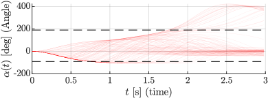
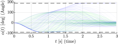
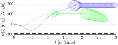
Figure 3: Comparison of closed-loop swing-up trajectories during 120 learning episodes under challenging position constraints (dashed lines). Top: Red lines show different learning episodes based on an unsafe learning policy. Middle: Closed-loop learning trajectories using a predictive safety filter with $10$ data points (green) and $18000$ data points (blue). Bottom: Resulting safe optimal closed-loop performance. The circle radii indicate the relative magnitude of safety ensuring modifications of the learning policy.

We consider the classical control problem of swinging up a pendulum from the downward position with angle $\alpha=0~{}\mathrm{[deg]}$ to the upward position ($\alpha=180~{}\mathrm{[deg]}$) with limited input authority, unknown system parameters, and under challenging safety constraints of the form $-90~{}\mathrm{[deg]}\leq\alpha\leq 190~{}\mathrm{[deg]}$, such that the pendulum is not allowed to tip over, once the upward position has been reached. The discretized dynamics $x(k+1)=f(x(k),u(k))$ are simulated using $x_{1}(k+1)=x_{1}(k)+hx_{2}(k)$ and $x_{2}(k+1)=x_{2}(k)-\frac{hg}{l}\sin(x_{1}(k))-\frac{h\eta}{ml^{2}}x_{2}(k)+\frac{h}{ml^{2}}u(k)$, where $x_{1}(k)=\alpha(k)$ is the angle, $x_{2}(k)=\dot{\alpha}(k)$ is the angular velocity at time step $k$, $h=0.02~{}\mathrm{[s]}$ is the discretization interval, $g=9.81~{}\mathrm{[m/s^{2}]}$ is the gravity constant, $l=0.5~{}\mathrm{[m]}$ is the length, $m=0.15~{}\mathrm{[kg]}$ is the mass, $\eta=0.1~{}\mathrm{[Nms/rad]}$ is the friction and the input torque $u$ is restricted to $|u|\leq 0.7~{}\mathrm{[Nms/rad]}$.
Unsafe learning policy $\pi_{\mathcal{L}}$: For learning the swing-up task, we consider an episodic learning setting with horizon length $\bar{N}=120$ and parametrize a bang-bang open-loop input signal as

$$\pi_{\mathcal{L}}(k;k_{s_{1}},k_{s_{2}})=\begin{cases}-0.7,\quad&k\leq k_{s_{1}},\\ 0.7,\quad&k_{s_{1}}\leq k\leq k_{s_{2}},\\ 0,&\text{else},\end{cases}$$ (17)

with switching times $k_{s_{1}}$ and $k_{s_{2}}$ subject to $k_{s_{1}}\in[0,k_{s_{2}}]$ and $k_{s_{2}}\in[0,150]$. The learning objective is defined as $\ell(x,k)=(\alpha(k)-\pi)^{2}+({v}^{*}_{0|k}-\pi_{\mathcal{L}}(k;k_{s_{1}},k_{s_{2}}))^{2}$, where the first term describes the distance to the desired upward position given by $180~{}\mathrm{[deg]}$, while the second term penalizes safety-ensuring interventions by the safety filter and therefore accelerates learning convergence as discussed in Akametalu et al. (2014). Efficient learning-based optimization of the parameters $k_{s_{1}}$ and $k_{s_{2}}$ is performed using Bayesian Optimization as described in Neumann-Brosig et al. (2019), selecting parameter configurations that automatically trade-off exploration of the parameter space and exploitation of promising subsets. While direct application of this learned policy yields a swing-up after some episodes, it causes significant constraint violations as shown in Figure 3 (top), motivating the application of the presented safety filter in the following.

Predictive safety filter from data: The transition model (1), (2) is obtained via linear Bayesian regression (Rasmussen and Williams, 2006), i.e., $f(x,u)=\theta^{\top}\phi(x)$, with $\phi(x,u)=[x_{1},x_{2},\sin(x_{1}),u]^{\top}$, unknown parameters $\theta\in\mathbb{R}^{2\times 4}$ with Gaussian priors, and Gaussian noise on obtained system measurements. The set-valued model confidence map according to Definition 4.4 for parametric uncertainties is given by (14) and can here be defined as $\mathcal{E}_{p_{\mathcal{S}}}(x,u)=\{e\in\mathbb{R}^{n}|e^{\top}\Sigma^{-1}(x,u)e\leq\chi_{2}^{2}(p_{\mathcal{S}})\}$ where $\Sigma(x,u)=\mathrm{diag}((\sigma_{i}^{2}(x,u))_{i=1,2})$ with $\sigma_{i}^{2}(x,u)$ being the posterior variance of $f_{i}(x,u)$ conditioned on data and $\chi_{2}^{2}(p_{\mathcal{S}})$ the chi-squared distribution of degree $2$ (Slotani, 1964). Starting with 10 data points around the downward position, we update the model belief using the acquired data after each episode. The tightening was experimentally chosen to $\rho=0.999,\epsilon=0.02$ using sampled system realizations of the posterior distribution as described in Section A.3. The corresponding admissible error set $\mathcal{E}^{\gamma}$ is defined as the $2$-norm ball with radius $\gamma=0.02$. Consequently, set-valued map constraints of the form $\mathcal{E}_{p_{\mathcal{S}}}(x,u)\subseteq\bar{\mathcal{E}}^{\gamma}_{i}$ according to (6e) can be efficiently implemented as $\sqrt{\sigma_{f_{j}}^{2}(x,u)\chi_{2}^{2}(p_{\mathcal{S}})}\leq(1-\epsilon_{i})0.02$ for $j=1,2$, i.e. by enforcing all semi-axes of $\mathcal{E}_{p_{\mathcal{S}}}(x,u)$ to be smaller or equal than the radius of the admissible error set $\bar{\mathcal{E}}^{0.02}_{i}$. The desired probability of chance constraint satisfaction $p_{\mathcal{S}}$ was chosen as $0.95$. As the terminal safe set, we select $\mathcal{S}^{t}\coloneqq\{\alpha,\dot{\alpha}|-30~{}\mathrm{deg}\leq\alpha\leq 30~{}\mathrm{[deg]},~{}|\dot{\alpha}|\leq 30~{}\mathrm{[deg/sec]}$ with $\pi_{\mathcal{S}}^{t}=0$. The resulting problem (6) with planning horizon $N=50$ was solved in real-time using Ipopt (Wächter and Biegler, 2006) together with the CasADi framework (Andersson et al., 2018) for automatic differentiation.

Results: Combining the learning-based swing up policy with a predictive safety filter based on only $10$ initial data points around the stable downward position results in cautious closed-loop system trajectories that are displayed as green lines in Figure 3 (middle). The corresponding optimal solution after 120 learning episodes is depicted in Figure 3 (middle). We can then leverage the cumulated data from the first experiment ($18000$ data samples) to refine the prediction model of the safety filter. The additional data enables a significantly less conservative learning behavior, see blue trajectories in Figure 3 (middle), and supports a complete swing-up, which demonstrates safe exploration beyond available data. The corresponding optimal solution after 120 learning episodes is shown in Figure 3 (middle), where the circle radii indicate the magnitude of safety ensuring modifications of the learning policy.

5.2 Safe data-driven quadrotor learning control

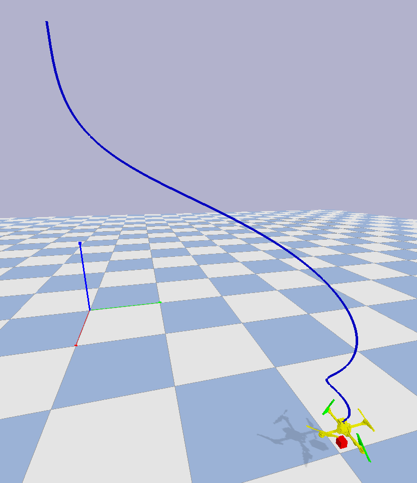
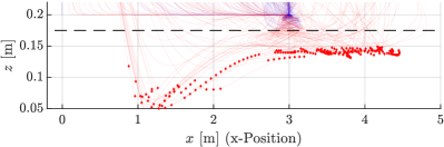
Figure 4: Quadrotor experiment using the Bullet Physics SDK (Coumans and Bai, 2016–2019). Top-left: Graphical interface showing the optimal safe trajectory (blue line). Top-right: Quadrotor trajectories projected on the $x-z$ plane using an unsafe policy search (red lines) and the safety augmented policy search (blue lines). Bottom: Zoom-in of top-right plot, where red dots represent states with $<0.01~{}\mathrm{[m]}$ minimum distance to the ground, which we classify as ground contact.

To demonstrate the presented method for a more challenging simulation example, we consider the AscTec Hummingbird drone, simulated in the Bullet Physics SDK (Coumans and Bai, 2016–2019), see Figure 4 (Top-left), in combination with a single rotor force model (Furrer et al., 2016). We employ a two-layer control structure, where an inner PD control loop takes desired pitch, roll and vertical acceleration in the body frame and outputs control signals to the motors. This enables modeling of the inner controlled system around the hovering equilibrium as done in Hu et al. (2018) using 10 states $\tilde{x}\in\mathbb{R}^{10}$, three inputs $u\in\mathbb{R}^{3}$, and dynamics of the form $\tilde{x}(k+1)=\theta^{\top}\phi(\tilde{x},u)$. State constraints are given by minimum height $z\geq 0.175~{}\mathrm{[m]}$ and maximal vertical velocity $|\dot{z}|\leq 1~{}\mathrm{[m/s]}$ to avoid ground contact and to ensure the validity of the dynamics model. The inputs to the inner control loop are normalized to $|u_{i}|\leq 1$.

Unsafe learning policy $\pi_{\mathcal{L}}$: The overall goal is to approach the landing position $x=3~{}\mathrm{[m]}$, $y=2~{}\mathrm{[m]}$, and $z=0.2~{}\mathrm{[m]}$ close to the ground, which is indicated by the red cube in Figure 4 (Top-left), starting from an initial hovering position at $z=3.5~{}\mathrm{[m]}$, $x=y=0~{}\mathrm{[m]}$ using an outer PD controller with state and input saturation, which is parametrized as

$$\pi_{\mathcal{L}}(\tilde{x};p,d)\coloneqq\begin{cases}\mathrm{clip}(p_{12}(x_{d}-x)+d_{12}\dot{x},-1,1)\\ \mathrm{clip}(p_{12}(y_{d}-y)+d_{12}\dot{y},-1,1)\\ \mathrm{clip}(p_{3}(z_{d}-z)+d_{3}\dot{z},-1,1)\end{cases}$$

where $\mathrm{clip}(x,c_{1},c_{2})\coloneqq\max(\min(x,c_{2}),c_{1})$ and with PD-controller gains $p_{12},p_{3}\in[0,10]$ and $d_{12},d_{3}\in[-10,0]$. Similar to the example presented in Section 5.1, we use Bayesian Optimization (Neumann-Brosig et al., 2019), with $\ell(\tilde{x},u)\coloneqq|x_{d}-x|+|y_{d}-y|+|z_{d}-z|+100\lVert{\pi_{\mathcal{L}}(\tilde{x})-{v}^{*}_{0|k}}\rVert_{2}$ that heavily penalizes safety ensuring actions by the safety filter. Direct application of the learning algorithm yields a significant number of ground contacts (in addition to violations of the maximum vertical velocity) as shown in Figure 4 by the red trajectories over a total of 240 learning episodes, where ground contacts are defined as $<0.01~{}\mathrm{[m]}$ minimum distance to the ground and are highlighted by red dots.

Predictive safety filter from data: Similarly to the numerical example in Section 5.1, we construct a model via Bayesian Regression using a Gaussian prior on the parameters $\theta$ together with Gaussian noise on observations. The data required for infering the prediction model is generated through experiments at a safe altitude using 100 random step inputs that are applied for $60~{}\mathrm{[s]}$ to the inner control loop. Based on the inferred model, the constraint tightening was experimentally chosen as $\rho=0.999,\epsilon=0.01$ using posterior samples as described in Section A.3 with a maximum allowable error set $\mathcal{E}^{\gamma}$ defined as the $2$-norm ball with radius $0.02$. The planning horizon is given by $N=20$ and the terminal set is selected as a sufficiently high altitude of $z\geq 1.5~{}\mathrm{[m]}$, from which we can guarantee constraint satisfaction for all future times using, e.g., suboptimal PD controller gains $p_{12}=p_{3}=0.5$ and $d_{12}=d_{3}=-0.5$. The set-valued model confidence map is set up analogue to Section 5.1 with desired chance constraint satisfaction $p_{\mathcal{S}}=0.9$.

Results: As shown in Figure 4 the predictive safety filter enables constraint satisfaction during all 240 learning-episodes and results in a favorable optimal trajectory as shown in Figure 4 (Top-left), for which the safety filter is permanently inactive as specified via the objective function.

6 Conclusion

This paper has addressed the problem of safe RL by introducing a predictive safety filter, which enables modularity in terms of safety and the employed RL algorithm. An optimization-based formulation was proposed that provides rigorous safety guarantees using a possibly data-driven approximate system model. By its capability to consider nonlinear and complex system descriptions without being overly conservative, we believe that the proposed approach is an important step towards safe RL for realistic applications.

Appendix A Appendix

A.1 Lipschitz continuity w.r.t. Hausdorff metric

Definition A.1.

The Hausdorff metric between two sets $\mathcal{A}$ and $\mathcal{B}$ in a metric space $(M,d_{\mathrm{M}})$ is defined as

$$d_{\mathrm{H}}(\mathcal{A},\mathcal{B})\coloneqq\max\left\{\adjustlimits{\sup}_{a\in\mathcal{A}}{\inf}_{b\in\mathcal{B}}d_{\mathrm{M}}(a,b),\adjustlimits{\inf}_{a\in\mathcal{A}}{\sup}_{b\in\mathcal{B}}d_{\mathrm{M}}(a,b)\right\}.$$

Definition A.2.

A set valued map $\mathcal{E}$ mapping vectors from $\mathcal{A}\subseteq\mathbb{R}^{n}$ to subsets of $\mathbb{R}^{m}$ is called Lipschitz continuous with Lipschitz constant $L_{\mathcal{E}}\geq 0$ under the Hausdorff metric with respect to the 2-Norm, if for all $a,b\in\mathcal{A}$ it holds that $d_{\mathrm{H}}(\mathcal{E}(a),\mathcal{E}(b))\leq L_{\mathcal{E}}\left\lVert{a-b}\right\rVert_{2}.$

A.2 Proof of Theorem 4.6

We begin by deriving a bound on the amount at which small changes in the planned nominal trajectory $\{{\mu}^{*}_{i|k},{v}^{*}_{i|k}\}$ affect the set membership constraint (6e) in Lemma A.3. Based on Assumption 4.3 together with Lipschitz continuity of the state, input, and terminal constraints, as well as the aforementioned bound on the set membership constraint, we then show that feasibility of (6) for planning horizon $N$ at time $k$ together with $e(k,\bar{\theta})\in\mathcal{E}_{p_{\mathcal{S}}}(x(k),u(k))$ implies the existence of a feasible solution at time $N-1$ in Lemma A.4. Finally, we iteratively apply Lemma A.4, to prove Theorem 4.6.

In the following, we consider a model error set $\mathcal{E}\coloneqq\{e\in\mathbb{R}^{n}|a_{\mathcal{E}}(e)\leq\mathbbm{1}_{n_{\mathcal{E}}}\}$, a safe terminal set $\mathcal{S}^{t}\coloneqq\{x\in\mathbb{R}^{n}|a_{\mathcal{S}}(x)\leq\mathbbm{1}_{n_{\mathcal{S}}}\}$ according to Assumption 4.2 with $a_{\mathcal{E},i}:\mathbb{R}^{n}\rightarrow\mathbb{R}$ and $a_{\mathcal{S},i}:\mathbb{R}^{n}\rightarrow\mathbb{R}$, both Lipschitz continuous functions with constants $L_{a_{\mathcal{E}}}$, $L_{a_{\mathcal{S}}}$. In the predictive safety filter optimization problem (6) the constraints are defined according to the tightening (9) and (16). We denote an optimal solution of (6) at time $k$ with planning horizon $N$ as nominal input sequence ${v}^{*}_{0|k,N},..,{v}^{*}_{N-1|k,N}$ with corresponding nominal state sequence ${\mu}^{*}_{0|k,N},..,{\mu}^{*}_{N|k,N}$ (6b).

Lemma A.3.

Let Assumption 4.5 hold. If $x,x^{+}\in\mathbb{X}$, $u,u^{+}\in\mathbb{U}$ and $\mathcal{E}_{p_{\mathcal{S}}}(x,u)\subseteq\mathcal{E}^{\gamma}$, then $\mathcal{E}_{p_{\mathcal{S}}}(x^{+},u^{+})\subseteq\mathcal{E}^{\gamma,+}(\left\lVert{\Delta z}\right\rVert_{2})$, where $\Delta z\coloneqq\left\lVert{[x^{\top},u^{\top}]-[x^{+\top},u^{+\top}]}\right\rVert_{2}$ and $\mathcal{E}^{\gamma,+}(\left\lVert{\Delta z}\right\rVert_{2})\coloneqq\{e\in\mathbb{R}^{n}|a_{\mathcal{E}}(e)\leq\gamma\mathbbm{1}_{n_{\mathcal{E}}}+L_{a_{\mathcal{E}}}L_{\mathcal{E}_{p_{\mathcal{S}}}}\left\lVert{\Delta z}\right\rVert_{2}\mathbbm{1}_{n_{\mathcal{E}}}\}$.

Proof.

The essential observation is that all $e^{+}\in\mathcal{E}_{p_{\mathcal{S}}}(x^{+},u^{+})$ can be written as $e^{+}=e^{*}+\Delta e$ with $e^{*}\coloneqq\operatorname*{arginf}_{e\in\mathcal{E}_{p_{\mathcal{S}}}(x,u)}\left\lVert{e^{+}-e}\right\rVert_{2}$, $\Delta e\in\mathbb{R}^{n}$ for which we have by Assumption 4.5 that

$$\left\lVert{\Delta e}\right\rVert_{2} =\left\lVert{e^{+}-e^{*}}\right\rVert_{2}=\inf_{e\in\mathcal{E}_{p_{\mathcal{S}}}(x,u)}{\left\lVert{e^{+}-e}\right\rVert_{2}}$$

$$\leq\adjustlimits{\sup}_{e^{+}\in\mathcal{E}_{p_{\mathcal{S}}}(x^{+},u^{+})}{\inf}_{e\in\mathcal{E}_{p_{\mathcal{S}}}(x,u)}{\left\lVert{e^{+}-e}\right\rVert_{2}}$$

$$\leq L_{\mathcal{E}_{p_{\mathcal{S}}}}\left\lVert{\Delta z}\right\rVert_{2}.$$

This allows us to derive

$$a_{\mathcal{E}}(e^{+}) =a_{\mathcal{E}}(e^{*})+a_{\mathcal{E}}(e^{+})-a_{\mathcal{E}}(e^{*})$$

$$\leq a_{\mathcal{E}}(e^{*})+L_{a_{\mathcal{E}}}\left\lVert{\Delta e}\right\rVert_{2}\mathbbm{1}_{n_{\mathcal{E}}}$$

$$\leq a_{\mathcal{E}}(e^{*})+L_{a_{\mathcal{E}}}L_{\mathcal{E}_{p_{\mathcal{S}}}}\left\lVert{\Delta z}\right\rVert_{2}\mathbbm{1}_{n_{\mathcal{E}}}$$

$$\leq\gamma\mathbbm{1}_{n_{\mathcal{E}}}+L_{a_{\mathcal{E}}}L_{\mathcal{E}_{p_{\mathcal{S}}}}\left\lVert{\Delta z}\right\rVert_{2}\mathbbm{1}_{n_{\mathcal{E}}}$$ (18)

since by definition $e^{*}\in\mathcal{E}_{p_{\mathcal{S}}}(x,u)\subseteq\mathcal{E}^{\gamma}$. Therefore, for all $e^{+}\in\mathcal{E}_{p_{\mathcal{S}}}(x^{+},u^{+})$, (18) holds, which implies $\mathcal{E}_{p_{\mathcal{S}}}(x^{+},u^{+})\subseteq\mathcal{E}^{\gamma,+}(\left\lVert{\Delta z}\right\rVert_{2})$, completing the proof. ∎

Lemma A.4.

Let Assumptions 4.3 and 4.5 hold. For every $\epsilon>0$, there exist corresponding $c>0,\gamma>0$ such that if 1) $L_{\mathcal{E}_{p_{\mathcal{S}}}}\leq c\epsilon$, 2) Problem (6) is feasible at time $k$ with prediction horizon $N>0$, 3) $u(k)=\pi_{\mathcal{S}}(k,x(k),u_{\mathcal{L}}(k))={v}^{*}_{0|k}$ is applied to (1), and 4) $e(k,\theta_{\mathcal{R}})\in\mathcal{E}_{p_{\mathcal{S}}}(x(k),u(k))$ with probability $1$, then the input sequence

$$\tilde{v}_{i|k+1}\coloneqq\pi(\tilde{\mu}_{i|k+1},{\mu}^{*}_{i+1|k,N},{v}^{*}_{i+1|k,N})~{}\text{ for }i\in\mathcal{I}_{[0,N-2]}$$

with $\pi$ according to Assumption 4.3, corresponding nominal state sequence $\tilde{\mu}_{i+1|k+1}=f(\tilde{\mu}_{i|k+1},\tilde{v}_{i|k+1},\bar{\theta})$ with $\tilde{\mu}_{0|k+1}=x(k+1)$ $\forall~{}i\in\mathcal{I}_{[0,N-2]}$ and $\tilde{\mu}_{-1|k+1}=x(k)$, is a feasible solution to (6) at time $k+1$ with prediction horizon $N-1$.

Proof.

The following proof is a modified and extended Version of Köhler et al. (2018b, Proposition 5), which considers nonlinear systems with additive disturbances of the form $x(k+1)=f(x(k),u(k))+w(k)$, to address model (1), (2) in combination with the set-valued model confidence and terminal safe set constraints (6e) and (6f). The proof makes use of the conditions in Assumption 4.3 to derive bounds on the difference between the optimal plan at time $k$, and the constructed plan $\{\tilde{\mu}_{i|k+1}\}$, $\{\tilde{v}_{i|k+1}\}$ at time $k+1$, which is in turn used to show that the constraint tightening implies that the constructed plan is a feasible solution for (6) with planning horizon $N-1$. In order to streamline notation, note that Assumption 4.3 holds for all $v,v^{+}\in\mathbb{U}$ which allows us, together with the fact that ${v}^{*}_{i|k}\in\mathbb{U}$ for all $i\in\mathcal{I}_{[0,N-1]}$ due to feasibility at time $k$, to omit the third argument of $V$ in the following analysis.

We start by bounding errors $e\in\mathcal{E}^{\gamma}$ in terms of the scaling factor $\gamma$ as defined in (12). Using the lower bound $\left\lVert{a_{\mathcal{E}}(e)}\right\rVert_{2}\geq c_{\mathcal{E}}\left\lVert{e}\right\rVert_{2}$ we obtain the relation $e\in\mathcal{E}^{\gamma}\Rightarrow a_{\mathcal{E}}(e)\leq\gamma\mathbbm{1}_{n_{\mathcal{E}}}\Rightarrow\|a_{\mathcal{E}}(e)\|_{\infty}\leq\gamma$, and it follows that

$$\text{for all }e\in\mathcal{E}^{\gamma}\text{ it holds }\left\lVert{e}\right\rVert_{2}\leq c_{\gamma}\gamma$$ (19)

with $c_{\gamma}\coloneqq(\sqrt{n_{\mathcal{E}}}/c_{\mathcal{E}})$. In the next step, we derive a bound $\gamma_{1}>0$ on $\gamma$ such that $V(x(k+1),{\mu}^{*}_{1|k,N})\leq\delta$ holds. Select $\gamma\leq\gamma_{1}\coloneqq c_{\gamma}^{-1}\sqrt{\frac{\delta}{c_{u}}}$ and note that by assumption and constraint (6e) we obtain

$$\left\lVert{x(k+1)-{\mu}^{*}_{1|k,N}}\right\rVert_{2}^{2}\leq c_{\gamma}^{2}\gamma^{2}\leq\frac{\delta}{c_{u}}$$ (20)

and combined with Assumption 4.3 it follows

$$V(x(k+1),{\mu}^{*}_{1|k,N}) \leq c_{u}\left\lVert{x(k+1)-{\mu}^{*}_{1|k,N}}\right\rVert_{2}^{2}\leq\delta.$$ (21)

Next, we show when $\gamma>0$ is small enough, $\tilde{v}_{i|k+1}$ is a feasible candidate input sequence to (6) with planning horizon $N-1$ in two steps. In Step 1 we show that $\tilde{\mu}_{i|k+1}\in\bar{\mathbb{X}}_{i}$ holds for all $i\in\mathcal{I}_{[0,N-2]}$ by induction, which allows us in Step 2 to construct sufficient bounds on $\gamma$ that imply feasibility via the tightening sequence (10) of the remaining constraints in (6).
Step 1: For the induction start $i=0$ we show $\tilde{\mu}_{0|k+1,N}\in\mathbb{X}_{0}=\mathbb{X}$ using the row sum norm $\left\lVert{A_{x}}\right\rVert_{\infty}$ and the fact that $\left\lVert{a}\right\rVert_{2}\left\lVert{b}\right\rVert_{2}\leq\left\lVert{a}\right\rVert_{1}\left\lVert{b}\right\rVert_{2}$ for all $a,b\in\mathbb{R}^{n_{x}}$ to get

$$A_{x}\tilde{\mu}_{0|k+1} =A_{x}{\mu}^{*}_{1|k,N}+A_{x}(\tilde{\mu}_{0|k+1}-{\mu}^{*}_{1|k,N})$$

$$\leq(1-\epsilon)\mathbbm{1}_{n_{x}}+\left\lVert{A_{x}}\right\rVert_{\infty}\left\lVert{\tilde{\mu}_{0|k+1}-{\mu}^{*}_{1|k,N}}\right\rVert_{2}\mathbbm{1}_{n_{x}}.$$

Since $V(\tilde{\mu}_{0|k+1},{\mu}^{*}_{1|k,N})\geq c_{l}||\tilde{\mu}_{0|k+1}-{\mu}^{*}_{1|k,N}||_{2}^{2}$ we have with (20), (21) that $||\tilde{\mu}_{0|k}-{\mu}^{*}_{1|k,N}||_{2}\leq\sqrt{\frac{c_{u}}{c_{l}}}c_{\gamma}\gamma$ and therefore $A_{x}\tilde{\mu}_{0|k+1}\leq(1-\epsilon)\mathbbm{1}_{n_{x}}+\left\lVert{A_{x}}\right\rVert_{\infty}\sqrt{\frac{c_{u}}{c_{l}}}c_{\gamma}\gamma\mathbbm{1}_{n_{x}}$. Selecting $\gamma\leq\gamma_{2}\coloneqq c_{\gamma}^{-1}\sqrt{\frac{c_{l}}{c_{u}}}\frac{\epsilon}{\left\lVert{A_{x}}\right\rVert_{\infty}}$ yields

$$A_{x}\tilde{\mu}_{0|k+1} \leq(1-\epsilon)\mathbbm{1}_{n_{x}}+\epsilon\mathbbm{1}_{n_{x}}\Rightarrow\tilde{\mu}_{0|k+1}\in\mathbb{X}.$$ (22)

In order to show the induction step $\forall j\in\mathcal{I}_{[0,i]}:~{}\tilde{\mu}_{j|k+1}\in\bar{\mathbb{X}}_{j}\Rightarrow\tilde{\mu}_{i+1|k+1}\in\bar{\mathbb{X}}_{i+1},$ for all $i\in\mathcal{I}_{[0,N-3]}$ we use Assumption 4.3 and derive

$$c_{u}c_{\gamma}^{2}\gamma^{2} \geq V(\tilde{\mu}_{0|k+1},{\mu}^{*}_{1|k,N})\geq\rho^{-1}V(\tilde{\mu}_{1|k+1},{\mu}^{*}_{2|k,N})\geq..$$

$$\geq\rho^{-i}V(\tilde{\mu}_{i|k+1},{\mu}^{*}_{i+1|k,N})$$

$$\geq\rho^{-1-i}V(\tilde{\mu}_{i+1|k+1},{\mu}^{*}_{i+2|k,N})$$

and consequently

$$V(\tilde{\mu}_{i+1|k+1},{\mu}^{*}_{i+2|k,N})\leq\rho^{i+1}c_{u}c_{\gamma}^{2}\gamma^{2}\leq\delta\text{ for all }i\in\mathcal{I}_{[0,N-3]}$$

since $\rho\in(0,1)$. By Assumption (4.3) we have $c_{l}||\tilde{\mu}_{i+1|k+1}-{\mu}^{*}_{i+2|k,N}||_{2}^{2}\leq V(\tilde{\mu}_{i+1|k+1},{\mu}^{*}_{i+2|k,N})$ and

$$\left\lVert{\tilde{\mu}_{i+1|k+1}-{\mu}^{*}_{i+2|k,N}}\right\rVert_{2}^{2} \leq\rho^{i+1}\frac{c_{u}}{c_{l}}c_{\gamma}^{2}\gamma^{2}.$$ (23)

Similar to (22) we can conclude with $\gamma\leq\gamma_{2}$ that

$$A_{x}\tilde{\mu}_{i+1|k+1} \leq A_{x}{\mu}^{*}_{i+2|k}+\left\lVert{A_{x}}\right\rVert_{\infty}\sqrt{\rho^{i+1}\frac{c_{u}}{c_{l}}}c_{\gamma}\gamma\mathbbm{1}_{n_{x}}$$

$$\leq(1-\epsilon_{i+2})\mathbbm{1}_{n_{x}}+\sqrt{\rho^{i+1}}\epsilon\mathbbm{1}_{n_{x}}$$

$$\leq(1-\epsilon_{i+1})\mathbbm{1}_{n_{x}}\Rightarrow\tilde{\mu}_{i+1|k+1}\in\bar{\mathbb{X}}_{i+1}$$

for all $i\in\mathcal{I}_{[0,N-3]}$, which proves constraint satisfaction of the candidate state sequence $\tilde{\mu}_{i|k+1}$ with respect to state constraints by induction.
Step 2: Regarding the terminal constraint (6f), note that due to $\tilde{\mu}_{N-2}\in\bar{\mathbb{X}}_{N-2}\subset\mathbb{X}$ we can use Assumption 4.3 similarly to before in order to obtain

$$\left\lVert{\tilde{\mu}_{N-1|k+1}-{\mu}^{*}_{N|k,N}}\right\rVert_{2}^{2} \leq\rho^{N-1}\frac{c_{u}}{c_{l}}c_{\gamma}^{2}\gamma^{2}.$$

Let $\gamma\leq\gamma_{3}\coloneqq c_{\gamma}^{-1}\sqrt{\frac{c_{l}}{c_{u}}}\frac{\epsilon}{L_{\mathcal{S}}}$, implying similarly

$$a_{\mathcal{S}}(\tilde{\mu}_{N-1|k+1}) \leq a_{\mathcal{S}}({\mu}^{*}_{N|k})+L_{\mathcal{S}}\sqrt{\rho^{N-1}\frac{c_{u}}{c_{l}}}c_{\gamma}\gamma\mathbbm{1}_{n_{s}}$$

$$\leq(1-\epsilon_{N-1})\mathbbm{1}_{n_{\mathcal{S}}},$$

showing terminal constraint satisfaction of (6f). Next we consider input constraints. Let $\gamma\leq\gamma_{4}\coloneqq c_{\gamma}^{-1}\sqrt{\frac{c_{l}}{c_{u}}}\frac{\epsilon}{\left\lVert{A_{u}}\right\rVert_{\infty}\pi_{\mathrm{max}}}$, yielding together with Assumption 4.3 and (23)

$$\left\lVert{\tilde{v}_{i|k+1}-{v}^{*}_{i+1|k,N}}\right\rVert_{2}^{2} \leq\pi_{\mathrm{max}}^{2}\left\lVert{\tilde{\mu}_{i|k+1}-{\mu}^{*}_{i+1|k,N}}\right\rVert_{2}^{2}$$

$$\leq\pi_{\mathrm{max}}^{2}\rho^{i}\frac{c_{u}}{c_{l}}c_{\gamma}^{2}\gamma^{2},$$

providing that

$$A_{u}\tilde{v}_{i|k+1} \leq A_{u}{v}^{*}_{i+1|k}+\left\lVert{A_{u}}\right\rVert_{\infty}\pi_{\mathrm{max}}\sqrt{\rho^{i}\frac{c_{u}}{c_{l}}}c_{\gamma}\gamma\mathbbm{1}_{n_{u}}$$

$$\leq(1-\epsilon_{i})\mathbbm{1}_{n_{u}}\text{ for all }i\in\mathcal{I}_{[0,N-2]},$$

showing input constraint satisfaction (6d) of the candidate input sequence. For the uncertainty constraint (6e) we have by Lemma A.3 that $\mathcal{E}_{p_{\mathcal{S}}}(\tilde{\mu}_{i|k+1},\tilde{v}_{i|k+1})\subseteq\bar{\mathcal{E}}_{i+1}^{\gamma,+}(\left\lVert{\Delta z_{i}}\right\rVert_{2})$ holds with $\bar{\mathcal{E}}_{i+1}^{\gamma,+}(\left\lVert{\Delta z_{i}}\right\rVert_{2})\coloneqq\{e\in\mathbb{R}^{n}|a_{\mathcal{E}}(e)\leq\gamma(1-\epsilon_{i+1})\mathbbm{1}_{n_{\mathcal{E}}}+L_{a_{\mathcal{E}}}L_{\mathcal{E}_{p_{\mathcal{S}}}}\left\lVert{\Delta z_{i}}\right\rVert_{2}\mathbbm{1}_{n_{\mathcal{E}}}\}$ and

$$\Delta z_{i} \coloneqq[{\tilde{\mu}_{i|k+1}}^{\top},{\tilde{v}_{i|k+1}}^{\top}]^{\top}-[{{\mu}^{*}_{i+1|k}}^{\top},{{v}^{*}_{i+1|k}}^{\top}]^{\top},$$

$$\left\lVert{\Delta z_{i}}\right\rVert_{2}^{2} \leq\left\lVert{\tilde{\mu}_{i|k+1}-{\mu}^{*}_{i+1|k}}\right\rVert_{2}^{2}+\left\lVert{\tilde{v}_{i|k+1}-{v}^{*}_{i+1|k}}\right\rVert_{2}^{2}$$

$$\leq(1+\pi_{\mathrm{max}})^{2}\rho^{i}\frac{c_{u}}{c_{l}}c_{\gamma}^{2}\gamma^{2}$$

for all $i\in\mathcal{I}_{[0,N-2]}$. For a sufficiently small Lipschitz constant in Assumption 4.5, such that $L_{\mathcal{E}_{p_{\mathcal{S}}}}\leq c\epsilon$ with

$$c\coloneqq\frac{1}{L_{a_{\mathcal{E}}}(1+\pi_{\mathrm{max}})}\sqrt{\frac{c_{l}}{c_{u}}}c_{\gamma}^{-1}$$ (24)

holds, we obtain

$$\mathcal{E}_{p_{\mathcal{S}}}(\tilde{\mu}_{i|k+1},\tilde{v}_{i|k+1})\subseteq\mathcal{E}_{i+1}^{\gamma,+}(\left\lVert{\Delta z}\right\rVert_{2})$$

$$~{}\subseteq\{e\in\mathbb{R}^{n}|a_{\mathcal{E}}(e)\leq\gamma(1-\epsilon_{i+1})\mathbbm{1}_{n_{\mathcal{E}}}$$

$$\qquad\qquad~{}~{}~{}~{}+L_{a_{\mathcal{E}}}L_{\mathcal{E}_{p_{\mathcal{S}}}}(1+\pi_{\mathrm{max}})\sqrt{\rho^{i}\frac{c_{u}}{c_{l}}}c_{\gamma}\gamma\mathbbm{1}_{n_{\mathcal{E}}}\}$$

$$~{}\subseteq\{e\in\mathbb{R}^{n}|a_{\mathcal{E}}(e)\leq\gamma(1-\epsilon_{i+1})\mathbbm{1}_{n_{\mathcal{E}}}+\sqrt{\rho^{i}}\epsilon\gamma\mathbbm{1}_{n_{\mathcal{E}}}\}$$

$$~{}\subseteq\{e\in\mathbb{R}^{n}|a_{\mathcal{E}}(e)\leq\gamma(1-\epsilon_{i})\mathbbm{1}_{n_{\mathcal{E}}}\}\subseteq\bar{\mathcal{E}}^{\gamma}_{i},$$

which shows feasibility of (6e). Therefore, if $L_{\mathcal{E}_{p_{\mathcal{S}}}}$ satisfies $L_{\mathcal{E}_{p_{\mathcal{S}}}}\leq c\epsilon$ for a selected $\epsilon$ with $c$ as defined in (24), then there always exists a

$$\gamma\coloneqq\min\{\gamma_{1},\gamma_{2},\gamma_{3},\gamma_{4}\}>0,$$ (25)

such that $\{\tilde{v}_{i|k+1}\}$ is a feasible solution to (6) at time $k+1$ with planning horizon $N-1$, proving the desired statement. ∎

Note that the bounds $\gamma_{i}$ for $i=1,2,3,4$ unveil an inner relationship between the constraint tightening fraction $\epsilon$ and the maximal allowable error set that is defined through the scaling parameter $\gamma$. Since the bound on $\gamma$ takes the form $\gamma\leq\min\{c_{\gamma}^{-1}\sqrt{\delta c_{u}^{-1}},\min_{i\in\{2,3,4\}}c_{i}\epsilon\}$ it follows that a bound exists on the error magnitude that can be tolerated depending on the size of the region, for which local incremental stabilizability according to Assumption 4.3 holds. Therefore, increasing the constraint tightening beyond $\epsilon=c_{\gamma}^{-1}\sqrt{\delta c_{u}^{-1}}/\min_{i}c_{i}$ will not necessarily allow an increase in the tolerable uncertainty magnitude. We can now utilize Lemma A.4 to prove Theorem 4.6, i.e. that application of Algorithm 2 implies safe system operation according to (4).

Proof of Theorem 4.6.

Select $\gamma$ according to Lemma A.4. By considering the different cases in Algorithm 2, we show safety $\forall k$ according to (4) by utilizing the relation

$$\Pr(\forall k:x(k)\in\mathbb{X},u(k)\in\mathbb{U})$$

$$\geq \Pr(\forall k:x(k)\in\mathbb{X},u(k)\in\mathbb{U},e(k,\theta_{\mathcal{R}})\in\mathcal{E}_{p_{\mathcal{S}}}(k))$$

$$= \Pr(\forall k:x(k)\in\mathbb{X},u(k)\in\mathbb{U}|\forall k:e(k,\theta_{\mathcal{R}})\in\mathcal{E}_{p_{\mathcal{S}}}(k))$$

$$\cdot\Pr(\forall k:e(k,\theta_{\mathcal{R}})\in\mathcal{E}_{p_{\mathcal{S}}}(k)),$$ (26)

where we use $\mathcal{E}_{p_{\mathcal{S}}}(k)$ instead of $\mathcal{E}_{p_{\mathcal{S}}}(x(k),u(k))$. Since $\Pr(\forall k:e(k,\theta_{\mathcal{R}})\in\mathcal{E}_{p_{\mathcal{S}}}(k))\geq p_{\mathcal{S}}$ by Assumption 4.5, relation (26) allows us to prove (3) by establishing

$$\Pr(\forall k:x(k)\in\mathbb{X},u(k)\in\mathbb{U}|\forall k:e(k,\theta_{\mathcal{R}})\in\mathcal{E}_{p_{\mathcal{S}}}(k))=1.$$ (27)

The proof therefore reduces to the deterministic case showing that $x(k)\in\mathbb{X}$, $u(k)\in\mathbb{U}$, given $e(k,\theta_{\mathcal{R}})\in\mathcal{E}_{p_{\mathcal{S}}}(k))$, at any time step $k$, which implies directly (27) for all times $k$ and therefore via (26) chance constraint satisfaction according to (4), i.e., safe system operation with respect to (4). In order to show $x(k)\in\mathbb{X}$ and $u(k)\in\mathbb{U}$, note that if (6) is feasible at time $k$ for any planning horizon $\tilde{N}>0$ it follows due to the state and input constraints (6c), (6d) that $x(k)\in\mathbb{X}$ and $u(k)\in\mathbb{U}$. This implies directly that $x(k)\in\mathbb{X}$ and $u(k)\in\mathbb{U}$ for any time step $k$ for which (6) is feasible for horizon $N$, as well as for all $\tilde{k}\in\mathcal{I}_{[k+1,N+k-1]}$, for which (6) is infeasible for horizon $N$, since feasibility of (6) with horizon $N-(\tilde{k}-k)$ is obtained from iteratively applying Lemma A.4 due to the condition that $\forall k:e(k,\theta_{\mathcal{R}})\in\mathcal{E}_{p_{\mathcal{S}}}(k)$. For all $\tilde{k}\geq N+k$, it follows from containment in the terminal safe set via (6f) and Assumption 4.2 that $x(\tilde{k})\in\mathbb{X}$ and $u(\tilde{k})=\pi_{\mathcal{S}}^{t}(x(k))\in\mathbb{U}$. This shows (27) and therefore via (26) that $\Pr(\forall k:x(k)\in\mathbb{X},u(k)\in\mathbb{U})\geq p_{\mathcal{S}}$, completing the proof. ∎

A.3 Offline design verification

The intuitive interpretation of the few parameters that need to be chosen allows to propose a selection and to certify it using sampling. Related statistical verification methods have been presented, e.g., in Hertneck et al. (2018); Karg et al. (2019). More precisely, to verify the underlying assumptions of Theorem 4.6 and to ensure that the admissible error, i.e. $\gamma$ in (12), is selected sufficiently small, we make use of a statistical offline verification procedure for finite horizon tasks, i.e. $\bar{N}<\infty$ in (3), for parameter design given a particular realization of a PSF $\pi_{\mathcal{S}}$ together with a learning policy $\pi_{\mathcal{L}}$. We sample and simulate a sufficiently large number $N_{\mathrm{total}}\in\mathbb{N}^{+}$ of system parameter realizations as well as initial conditions according to their distributions $p(\theta)$ and $p(x_{\mathrm{init}})$ and provide a statistical bound on the number of successful simulations that ensure safety according to (4). Let $\theta^{(j)}\sim p(\theta)$ and $x_{\mathrm{init}}^{(j)}\sim p(x_{\mathrm{init}})$ for $j=1,2,..,N_{\mathrm{total}}$ be i.i.d. samples and define an indicator function for safe execution as

$$\mathbb{I}(\theta^{(j)},x_{\mathrm{init}}^{(j)})=\begin{cases}1,\forall k=1,..,\bar{N}:&x_{\mathrm{init}}^{(j)}(k)\in\mathbb{X}~{}\land\\ &\pi_{\mathcal{L}}(k,x_{\mathrm{init}}^{(j)}(k))\in\mathbb{U}\\ 0,&\text{otherwise}\end{cases}$$

with sampled system dynamics of the form $x_{\mathrm{init}}^{(j)}(k+1)=f(x_{\mathrm{init}}^{(j)}(k),\pi_{\mathcal{L}}(k,x_{\mathrm{init}}^{(j)}(k));\theta^{(j)})$ and initial condition $x_{\mathrm{init}}^{(j)}(0)=x_{\mathrm{init}}^{(j)}$. The probability of satisfying constraints $\mathbb{X}$ and $\mathbb{U}$ can therefore be expressed as $p_{\mathcal{S}}^{\infty}\coloneqq\lim_{N_{\mathrm{total}}\rightarrow\infty}\bar{p}_{\mathcal{S}}(N_{\mathrm{total}})$ with

$$\bar{p}_{\mathcal{S}}(N_{\mathrm{total}})\coloneqq N_{\mathrm{total}}^{-1}\sum_{j=0}^{N_{\mathrm{total}}}\mathbb{I}(\theta^{(j)},x_{\mathrm{init}}^{(j)})$$

via the law of large numbers. To determine a sufficiently large but finite number $N_{\mathrm{total}}$ to ensure $p_{\mathcal{S}}^{\infty}\geq p_{\mathcal{S}}$ we use Hoeffding’s inequality (von Luxburg and Schölkopf; 2011, Section 4.1) as similarly proposed in Hertneck et al. (2018): $\Pr(|p_{\mathcal{S}}^{\infty}-\bar{p}_{\mathcal{S}}(N_{\mathrm{total}})|\geq\Delta_{H}^{2})\leq 2\exp(-2N_{\mathrm{total}}\Delta_{H})$ for an error margin $\Delta_{H}>0$. By defining $\delta_{H}\coloneqq 2\exp(-2N_{\mathrm{total}}\Delta_{H})$ it follows that $p_{\mathcal{S}}^{\infty}\geq p_{\mathcal{S}}(N_{\mathrm{total}})+\Delta_{H}$ holds at confidence level $1-\delta_{H}$. This allows us to state a formal lower bound on the total number of offline simulations as follows:

Proposition A.5.

Consider a specific PSF problem parametrization, learning policy $\pi_{\mathcal{L}}$, and confidence level $1-\delta_{H}$. If $\bar{p}_{\mathcal{S}}(N_{\mathrm{total}})>p_{\mathcal{S}}$ holds and

$$N_{\mathrm{total}}\geq-\frac{\log(0.5\delta_{H})}{2(\bar{p}_{\mathcal{S}}(N_{\mathrm{total}})-p_{\mathcal{S}})^{2}},$$ (28)

then the chance constraints (4) are fulfilled under application of $u(k)=\pi_{\mathcal{S}}(k,x(k),\pi_{\mathcal{L}}(k,x(k)))$ to the real system (1).

For example, if we have $p_{\mathcal{S}}=0.95$ and $\bar{p}_{\mathcal{S}}(N_{\mathrm{total}})=0.99$ for a specific choice of design parameters, then $N_{\mathrm{total}}$ needs to be greater than $1656$ to provide a sound PSF parametrization with $99\%$ confidence. Note that (28) is independent of the complexity of the system and that offline simulations can be executed in parallel. Naturally, small required values of $|p_{\mathcal{S}}-\bar{p}_{\mathcal{S}}(N_{\mathrm{total}})|$ can lead to a rapid increase of $N_{\mathrm{total}}$. In case of infeasibility one needs to re-adjust the design parameters as described in Section 4.3 or more data needs to be collected.

A.4 Sufficient condition for Assumption 4.3

Different from Köhler et al. (2018a, b) we require the first condition in Assumption 4.3 to also hold for the case that $V(x,z,v)>\delta$, which is used in the proof of Lemma A.4. Nevertheless, Köhler et al. (2018a, Prop. 1) still implies that the following verifiable assumption is sufficient for Assumption 4.3 and relates it to local stabilizability of system (1).

Assumption A.6.

Let $r\coloneqq(\mu,v)\in\mathbb{X}\times\mathbb{U}$ and define the linearization $A_{r}\coloneqq\tfrac{\partial f}{\partial x}(r,\bar{\theta})$, $B_{r}\coloneqq\tfrac{\partial f}{\partial u}(r,\bar{\theta})$. For any $r\in\mathbb{X}\times\mathbb{U}$, the pair $(A_{r},B_{r})$ is stabilizable, i.e. there exist $K_{r}\in\mathbb{R}^{m\times n}$, $P_{r},Q_{r}\in\mathbb{R}^{n\times n}$ positive definite and continuous in $r$, such that

$$P_{r}-(A_{r}+B_{r}K_{r})^{\top}P_{r}(A_{r}+B_{r}K_{r})=Q_{r}.$$ (29)

Furthermore, there exists a constant $c\in\mathbb{R}_{>0}$, such that for any $r^{+}=(\mu^{+},v^{+})\in\mathbb{X}\times\mathbb{U}$ with $\mu^{+}=f(\mu,v,\bar{\theta})$, the corresponding matrix $P_{r^{+}}$ satisfies:

$$\lambda_{\mathrm{max}}(P_{r}^{-1}P_{r^{+}})Q_{r}\geq(\lambda_{\mathrm{max}}(P_{r}^{-1}P_{r^{+}})-1)P_{r}+cI_{n}.$$ (30)

Given Assumption A.6, we can choose $V(x,\mu,v)=(x-\mu)^{\top}P_{r}(x-\mu)$ in Assumption 4.3, with (30) bounding the rate at which $V(x,\mu,v)$ can possibly change in any time step when applying $u=\pi(x,\mu,v)=v+K_{r}(x-\mu)$. Note that, according to Köhler et al. (2018a, Prop. 1), Assumption A.6 is only sufficient for Assumption 4.3, and therefore stabilizability of the linearization along any reference might not be needed in practice. However, it allows us to analytically express conditions that can be verified in principled steps. While (29) is always satisfied as long as the system is locally stabilizable, the second equation accounts for linearization errors as the system evolves and can therefore be seen as an intrinsic consequence of a local linearization-based analysis. As a practical consequence, the condition might be too conservative for nonlinear systems with quickly changing linearizations along references, i.e. large $||(A_{r+1},B_{r+1})-(A_{r},B_{r})||$. See, e.g., Köhler et al. (2018a, b) for concrete examples that demonstrate how Assumption A.6 can be verified for different nonlinear systems.

References

- (1)
- Achiam et al. (2017) Achiam, J., Held, D., Tamar, A. and Abbeel, P. (2017). Constrained policy optimization, International Conference on Machine Learning, pp. 22–31.
- Akametalu et al. (2014) Akametalu, A. K., Kaynama, S., Fisac, J. F., Zeilinger, M. N., Gillula, J. H. and Tomlin, C. J. (2014). Reachability-based safe learning with Gaussian processes, Proceedings of the IEEE Conference on Decision and Control, IEEE, pp. 1424–1431.
- Ames et al. (2019) Ames, A. D., Coogan, S., Egerstedt, M., Notomista, G., Sreenath, K. and Tabuada, P. (2019). Control barrier functions: Theory and applications, 2019 18th European Control Conference, ECC 2019 pp. 3420–3431.
- Ames et al. (2017) Ames, A. D., Xu, X., Grizzle, J. W. and Tabuada, P. (2017). Control Barrier Function Based Quadratic Programs for Safety Critical Systems, IEEE Transactions on Automatic Control 62(8): 3861–3876.
- Amodei et al. (2016) Amodei, D., Olah, C., Steinhardt, J., Christiano, P., Schulman, J. and Mané, D. (2016). Concrete problems in AI safety, arXiv preprint arXiv:1606.06565 .
- Andersson et al. (2018) Andersson, J. A. E., Gillis, J., Horn, G., Rawlings, J. B. and Diehl, M. (2018). CasADi – A software framework for nonlinear optimization and optimal control, Mathematical Programming Computation .
- Berkenkamp et al. (2016) Berkenkamp, F., Moriconi, R., Schoellig, A. P. and Krause, A. (2016). Safe learning of regions of attraction for uncertain, nonlinear systems with Gaussian Processes, 55th IEEE Conference on Decision and Control (CDC), pp. 4661–4666.
- Bouffard et al. (2012) Bouffard, P., Aswani, A. and Tomlin, C. (2012). Learning-based model predictive control on a quadrotor: Onboard implementation and experimental results, 2012 IEEE International Conference on Robotics and Automation, pp. 279–284.
- Chen and Allgöwer (1998) Chen, H. and Allgöwer, F. (1998). A quasi-infinite horizon nonlinear model predictive control scheme with guaranteed stability, Automatica 34(10): 1205 – 1217.
- Chowdhury and Gopalan (2017) Chowdhury, S. R. and Gopalan, A. (2017). On kernelized multi-armed bandits, International Conference on Machine Learning (ICML), pp. 844–853.
- Coumans and Bai (2016–2019) Coumans, E. and Bai, Y. (2016–2019). Pybullet, a python module for physics simulation for games, robotics and machine learning.
- Domahidi et al. (2012) Domahidi, A., Zgraggen, A. U., Zeilinger, M. N., Morari, M. and Jones, C. N. (2012). Efficient interior point methods for multistage problems arising in receding horizon control, 51st IEEE Conference on Decision and Control (CDC), pp. 668–674.
- Fisac et al. (2019) Fisac, J. F., Akametalu, A. K., Zeilinger, M. N., Kaynama, S., Gillula, J. and Tomlin, C. J. (2019). A General Safety Framework for Learning-Based Control in Uncertain Robotic Systems, IEEE Transactions on Automatic Control 64(7): 2737–2752.
- Furrer et al. (2016) Furrer, F., Burri, M., Achtelik, M. and Siegwart, R. (2016). RotorS-A modular gazebo MAV simulator framework, Studies in Computational Intelligence 625: 595–625.
- Garcıa and Fernández (2015) Garcıa, J. and Fernández, F. (2015). A comprehensive survey on safe reinforcement learning, Journal of Machine Learning Research 16: 1437–1480.
- Gillula and Tomlin (2011) Gillula, J. H. and Tomlin, C. J. (2011). Guaranteed safe online learning of a bounded system, Intelligent Robots and Systems (IROS), 2011 IEEE/RSJ International Conference on, IEEE, pp. 2979–2984.
- Grune and Palma (2014) Grune, L. and Palma, V. G. (2014). On the Benefit of Re-optimization in Optimal Control under Perturbations, Proceedings of the 21st International Symposium on Mathematical Theory of Networks and Systems – MTNS 2014 pp. 439–446.
- Hertneck et al. (2018) Hertneck, M., Kohler, J., Trimpe, S. and Allgöwer, F. (2018). Learning an Approximate Model Predictive Controller with Guarantees, IEEE Control Systems Letters 2(3): 543–548.
- Hewing et al. (2018) Hewing, L., Liniger, A. and Zeilinger, M. N. (2018). Cautious NMPC with Gaussian process dynamics for autonomous miniature race cars, 2018 European Control Conference (ECC), IEEE, pp. 1341–1348.
- Hewing et al. (2020) Hewing, L., Wabersich, K. P., Menner, M. and Zeilinger, M. N. (2020). Learning-Based Model Predictive Control: Toward Safe Learning in Control, Annual Review of Control, Robotics, and Autonomous Systems 3(1).
- Hu et al. (2018) Hu, H., Feng, X., Quirynen, R., Villanueva, M. E. and Houska, B. (2018). Real-Time Tube MPC Applied to a 10-State Quadrotor Model, Proceedings of the American Control Conference, IEEE, pp. 3135–3140.
- Kamthe and Deisenroth (2017) Kamthe, S. and Deisenroth, M. P. (2017). Data-efficient reinforcement learning with probabilistic model predictive control, arXiv preprint arXiv:1706.06491 .
- Karg et al. (2019) Karg, B., Alamo, T. and Lucia, S. (2019). Probabilistic performance validation of deep learning-based robust NMPC controllers, arXiv preprint arXiv:1910.13906 .
- Köhler et al. (2018a) Köhler, J., Müller, M. A. and Allgöwer, F. (2018a). Nonlinear reference tracking: An economic model predictive control perspective, IEEE Transactions on Automatic Control pp. 1–1.
- Köhler et al. (2018b) Köhler, J., Müller, M. A. and Allgöwer, F. (2018b). A novel constraint tightening approach for nonlinear robust model predictive control, 2018 Annual American Control Conference (ACC), pp. 728–734.
- Koller et al. (2018) Koller, T., Berkenkamp, F., Turchetta, M. and Krause, A. (2018). Learning-based model predictive control for safe exploration, 2018 IEEE Conference on Decision and Control (CDC), IEEE, pp. 6059–6066.
- Levine et al. (2016) Levine, S., Finn, C., Darrell, T. and Abbeel, P. (2016). End-to-end training of deep visuomotor policies, The Journal of Machine Learning Research 17: 1334–1373.
- Li and Bastani (2019) Li, S. and Bastani, O. (2019). Robust model predictive shielding for safe reinforcement learning with stochastic dynamics, arXiv preprint arXiv:1910.10885 .
- Limon et al. (2017) Limon, D., Calliess, J. and Maciejowski, J. (2017). Learning-based nonlinear model predictive control, IFAC-PapersOnLine 50(1): 7769 – 7776.
- Majumdar and Tedrake (2017) Majumdar, A. and Tedrake, R. (2017). Funnel libraries for real-time robust feedback motion planning, The International Journal of Robotics Research 36(8): 947–982.
- Mannucci et al. (2018) Mannucci, T., van Kampen, E. J., de Visser, C. and Chu, Q. (2018). Safe exploration algorithms for reinforcement learning controllers, IEEE Transactions on Neural Networks and Learning Systems PP: 1–13.
- Mayne (2014) Mayne, D. Q. (2014). Model predictive control: Recent developments and future promise, Automatica 50(12): 2967–2986.
- Neumann-Brosig et al. (2019) Neumann-Brosig, M., Marco, A., Schwarzmann, D. and Trimpe, S. (2019). Data-Efficient Autotuning With Bayesian Optimization: An Industrial Control Study, IEEE Transactions on Control Systems Technology pp. 1–11.
- Ohnishi et al. (2019) Ohnishi, M., Wang, L., Notomista, G. and Egerstedt, M. (2019). Barrier-Certified Adaptive Reinforcement Learning With Applications to Brushbot Navigation, IEEE Transactions on Robotics 35(5): 1186–1205.
- Ostafew et al. (2016) Ostafew, C. J., Schoellig, A. P. and Barfoot, T. D. (2016). Robust constrained learning-based NMPC enabling reliable mobile robot path tracking, The International Journal of Robotics Research 35(13): 1547–1563.
- Prajna and Jadbabaic (2004) Prajna, S. and Jadbabaic, A. (2004). Safety verification of hybrid systems using barrier certificates, Lecture Notes in Computer Science 2993: 477–492.
- Rasmussen and Williams (2006) Rasmussen, C. and Williams, C. (2006). Gaussian Processes for Machine Learning, Adaptive Computation and Machine Learning, MIT Press.
- Seto et al. (1998) Seto, D., Krogh, B., Sha, L. and Chutinan, A. (1998). The simplex architecture for safe on-line control system upgrades, Proceedings of the American Control Conference, Vol. 6, IEEE, pp. 3504–3508.
- Slotani (1964) Slotani, M. (1964). Tolerance regions for a multivariate normal population, Annals of the Institute of Statistical Mathematics 16(1): 135–153.
- Soloperto et al. (2018) Soloperto, R., Müller, M. A., Trimpe, S. and Allgöwer, F. (2018). Learning-based robust model predictive control with state-dependent uncertainty, IFAC-PapersOnLine 51(20): 442–447.
- Tanaskovic et al. (2013) Tanaskovic, M., Fagiano, L., Smith, R., Goulart, P. and Morari, M. (2013). Adaptive model predictive control for constrained linear systems, Control Conference (ECC), 2013 European, IEEE, pp. 382–387.
- Tedrake et al. (2010) Tedrake, R., Manchester, I. R., Tobenkin, M. and Roberts, J. W. (2010). LQR-trees: Feedback motion planning via sums-of-squares verification, The International Journal of Robotics Research 29(8): 1038–1052.
- Thomas et al. (1994) Thomas, M. M., Kardos, J. L. and Joseph, B. (1994). Shrinking horizon model predictive control applied to autoclave curing of composite laminate materials, Proceedings of the American Control Conference.
- von Luxburg and Schölkopf (2011) von Luxburg, U. and Schölkopf, B. (2011). Statistical Learning Theory: Models, Concepts, and Results.
- Wabersich and Zeilinger (2018a) Wabersich, K. P. and Zeilinger, M. N. (2018a). Linear model predictive safety certification for learning-based control, 2018 IEEE Conference on Decision and Control (CDC), IEEE, pp. 7130–7135.
- Wabersich and Zeilinger (2018b) Wabersich, K. P. and Zeilinger, M. N. (2018b). Scalable synthesis of safety certificates from data with application to learning-based control, 2018 European Control Conference (ECC), pp. 1691–1697.
- Wächter and Biegler (2006) Wächter, A. and Biegler, L. T. (2006). On the implementation of an interior-point filter line-search algorithm for large-scale nonlinear programming, Mathematical programming 106(1): 25–57.
- Wang et al. (2018) Wang, L., Han, D. and Egerstedt, M. (2018). Permissive Barrier Certificates for Safe Stabilization Using Sum-of-squares, Proceedings of the American Control Conference 2018-June: 585–590.
- Wieland and Allgöwer (2007) Wieland, P. and Allgöwer, F. (2007). Constructive safety using control barrier functions, IFAC Proceedings Volumes 40(12): 462–467.