LISA Pathfinder Platform Stability and Drag-free Performance

Abstract

The science operations of the LISA Pathfinder mission has demonstrated the feasibility of sub-femto-g free-fall of macroscopic test masses necessary to build a LISA-like gravitational wave observatory in space. While the main focus of interest, i.e. the optical axis or the $\displaystyle x$-axis, has been extensively studied, it is also of interest to evaluate the stability of the spacecraft with respect to all the other degrees of freedom. The current paper is dedicated to such a study, with a focus set on an exhaustive and quantitative evaluation of the imperfections and dynamical effects that impact the stability with respect to its local geodesic. A model of the complete closed-loop system provides a comprehensive understanding of each part of the in-loop coordinates spectra. As will be presented, this model gives very good agreements with LISA Pathfinder flight data. It allows one to identify the physical noise source at the origin and the physical phenomena underlying the couplings. From this, the performances of the stability of the spacecraft, with respect to its geodesic, are extracted as a function of frequency. Close to $\displaystyle 1mHz$, the stability of the spacecraft on the $\displaystyle X_{SC}$, $\displaystyle Y_{SC}$ and $\displaystyle Z_{SC}$ degrees of freedom is shown to be of the order of $\displaystyle 5.0\ 10^{-15}m\ s^{-2}/\sqrt{Hz}$ for X and $\displaystyle 4.0\ 10^{-14}m\ s^{-2}/\sqrt{Hz}$ for Y and Z. For the angular degrees of freedom, the values are of the order $\displaystyle 3\ 10^{-12}rad\ s^{-2}/\sqrt{Hz}$ for $\displaystyle\Theta_{SC}$ and $\displaystyle 3\ 10^{-13}rad\ s^{-2}/\sqrt{Hz}$ for $\displaystyle H_{SC}$ and $\displaystyle\Phi_{SC}$. Below $\displaystyle 1mHz$, however, the stability performances are observed to be significantly deteriorated, because of the important impact of the star tracker noise on the closed loop system. It is worth noting that LISA is expected to be spared from such concerns, essentially as Differential Wave-front Sensing, an attitude sensor system of much higher precision, will be utilized for attitude control.

I.  General Introduction

The stability of a space platform, understood as a property of low noise acceleration of the platform with respect to the local geodesic, is a quality that is often searched for in order to satisfy the requirements of scientific observations or to perform tests of fundamental physics. Examples of such activity range from high precision geodesy, gravity field and gradient measurements (GRACE, GOCE), experimental test of gravitation (GP-B, MICROSCOPE) and gravitational wave astronomy (LISA Pathfinder, LISA). Using two quasi free-falling test masses (TMs), LISA Pathfinder (LPF) Anza et al. (2005) has demonstrated remarkable properties related to its stability and recent publications (see Armano et al. (2016) and Armano et al. (2018)) have presented the observed performance along the axis joining its test masses. However, the importance of the stability of the LISA Pathfinder platform is not limited to this axis, therefore in this paper we present results associated to its 6 degrees of freedom. In order to evaluate these performance, it is necessary not only to make use of the internal measurement of its sensors and actuators but also to deduce the true motion of the spacecraft S/C impacted by the imperfections of the sensor and actuator systems. Beyond this, it is also necessary to evaluate the relative motion between the test masses and the platform due to internal forces whose manifestation is hidden from most sensors because the closed-loop control scheme nulls the measurement of in-loop sensors on LISA Pathfinder. In this publication we first introduce the configuration of the LISA Pathfinder platform and then the closed-loop control scheme that allows the observed performance to be reached. In order to understand how these performance are reached, we introduce a simplified linear time invariant State Space model which allows extrapolation from in-loop sensor outputs in order to obtain needed physical quantities otherwise unobserved. An important example of such quantity is the actual low frequency relative displacement between the test masses and the S/C, driven by the sensors noise and masked by fundamental properties of the closed-loop systems (further details at section VII). We show that this model is capable of reproducing the observations of the sensors to within a few percent and can therefore be relied upon. The last section, before the conclusion, is devoted to summing up all the effects that allow the stability of LPF w.r.t. its local geodesic over the six degrees of freedom to be deduced.

II.  The LISA Pathfinder Platform

LISA Pathfinder Armano et al. (2015) aims to demonstrate that it is technically possible to make inertial reference frames in space at the precision required by low-frequency gravitational waves astronomy. Indeed, in a LISA-like observatory design Amaro-Seoane et al. (2017), one needs excellent references of inertia inside each satellites in order to differentiate between spurious accelerations of the apparatus from gravitational radiations, which both result in detected oscillatory variation of the arm lengths of the spacecraft constellation. The quality of free-fall achieved along the $\displaystyle X$-axis, the axis of main interest (i.e. representing axes along LISA arms), has already significantly exceeded expectations Armano et al. (2016). In addition to limiting stray forces acting directly on the TM, the LPF differential acceleration result required stringent and specific control of the TM-SC relative motion, to limit elastic ”stiffness” coupling and possible cross-talk effects. Besides, post=processing software corrections from modeling of such S/C-to-TM acceleration couplings have been proven to be necessary and efficient in order to extract measurements of residual acceleration exerted on the TMs only (such as inertial forces, stiffness coupling, cross-talk corrections Armano et al. (2016)).

The control scheme required challenging technologies permitting high precision sensing and actuation in order to finely track and act on the three bodies and keep them at their working point. LISA Technology Package (LTP), the main payload of LISA Pathfinder, was built to demonstrate the required performance Armano et al. (2015) and includes high performance sensing and actuation subsystems. The Gravitational Reference Sensor (GRS) Dolesi et al. (2003) includes the $\displaystyle 1.93$\displaystyle\mathrm{k}\mathrm{g}$$ Au-Pt test mass, surrounded by a conducting electrostatic shield with electrodes that are used for simultaneous capacitive position sensing and electrostatic force actuation of the TM. The Optical Metrology System (OMS) Heinzel et al. (2004) uses heterodyne interferometry for high precision test mass displacement measurements. Angular displacements are sensed through the Differential Wavefront System (DWS) using phase differences measured across the four quadrants of photodiodes. Star Trackers (ST) orients the spacecraft w.r.t. to a Galilean frame and the micro-thruster system, a set of six Cold-Gas micro-thrusters (a technology already flown in space with ESA’s GAIA mission Brown et al. (2016) and CNES’s Microscope mission Touboul et al. (2017)), allows S/C displacement and attitude control along its six degrees of freedom. Note that LISA Pathfinder also has a NASA participation, contributing a set of 8 Colloidal Thrusters and the electronics/computer that control them Anderson et al. (2018).

Figure 1: Simplified sketch of LISA Pathfinder apparatus. The system of coordinates used to describe the displacement of the test masses (purple sets of axes) and of the spacecraft (green set of axes) are made explicit.

III.  The Drag-Free and Attitude Control System (DFACS)

The Drag-Free and Attitude Control System (DFACS) Fichter et al. (2005) is a central subsystem in LISA Pathfinder architecture. It has been designed by Airbus Defence & Space Schleicher and al (2017). It is devoted to achieve the control scheme that maintains the test masses to be free-falling at the centre of their electrode housings (translation control), to keep a precise alignment of the TMs w.r.t. the housing inner surfaces (rotation control) and to track the desired spacecraft orientation w.r.t. inertial frames (spacecraft attitude control). The translational control strategy is designed to limit any applied electrostatic suspension forces on the TMs to the minimum necessary to compensate any differential acceleration between the two TMs, while common mode motion of these geodesic references, which essentially reflects S/C accelerations, is drag-free controlled with the micro-thrusters. Limiting the applied actuation forces limits a critical acceleration noise from the actuator gain noise. This drag-free control is essentially used to counterbalance the noisy motion of the spacecraft, which is both exposed to the space environment and largely to its own thrust noise. A linear combination of test mass coordinates inside their housing along $\displaystyle Y-$ and $\displaystyle Z-$ axes are preferred for drag-free control, translational thrust being used to correct common-mode displacements while rotational actuations are performed to correct differential-mode displacements (see table 1, entries 5-8). Due to the geometrical configuration of the experiment (see figure 1), differential $\displaystyle x-$displacements of the TMs cannot be corrected by the drag-free control. In this case, it is necessary to apply control forces on one of the TMs along the $\displaystyle X$-axis. The strategy used is to leave TM1 in pure free-fall while the second mass is forced to follow the first, in order to keep the relative position of the masses constant at low frequencies. The amount of electrostatic force required to achieve this is measured and accounted for in the computation of the acceleration noise experienced by the masses Armano et al. (2016). This control scheme is called suspension control. All the angular coordinates of the test masses (except rotation around $\displaystyle x_{\scriptscriptstyle 1}$) are controlled by the suspension control scheme (see table 1). The attitude of the spacecraft w.r.t. Galilean frame are supported by the attitude control. Because the commanded torques on the satellite are driven by the drag-free control of the differential linear displacement of the masses along $\displaystyle Y-$ and $\displaystyle Z-$ axes, as previously mentioned, the attitude control is realized indirectly. First, the attitude control demands differential forces on the masses according to information coming from the star trackers. Then, the drag-free loop takes the baton and corrects the induced differential displacement by requiring a rotation of the spacecraft, thus executing the rotation imposed by the star trackers.

Table 1: Control scheme of LISA Pathfinder in nominal science mode. For each system’s dynamical coordinate, the table lists by which subsystem it is sensed, its associated control type and the actuator used. $\displaystyle d$ is the distance between the TMs

#	Coordinates	Sensor system	Control Mode	Actuation system
1	$\displaystyle\Theta$	ST	Attitude	GRS ($\displaystyle Tx_{\scriptscriptstyle 1}$)
2	$\displaystyle H$	ST	Attitude	GRS ($\displaystyle Fz_{\scriptscriptstyle 2}-Fz_{\scriptscriptstyle 1}$)
3	$\displaystyle\Phi$	ST	Attitude	GRS ($\displaystyle Fy_{\scriptscriptstyle 2}-Fy_{\scriptscriptstyle 1}$)
4	$\displaystyle x_{\scriptscriptstyle 1}$	IFO	Drag-Free	$\displaystyle\mu$-thrust ($\displaystyle\uparrow$ X-axis)
5	$\displaystyle\frac{y_{\scriptscriptstyle 2}+y_{\scriptscriptstyle 1}}{2}$	GRS	Drag-Free	$\displaystyle\mu$-thrust ($\displaystyle\uparrow$ Y-axis)
6	$\displaystyle\frac{z_{\scriptscriptstyle 2}+z_{\scriptscriptstyle 1}}{2}$	GRS	Drag-Free	$\displaystyle\mu$-thrust ($\displaystyle\uparrow$ Z-axis)
7	$\displaystyle\frac{y_{\scriptscriptstyle 2}-y_{\scriptscriptstyle 1}}{d}$	GRS	Drag-Free	$\displaystyle\mu$-thrust ($\displaystyle\circlearrowleft$ Z-axis)
8	$\displaystyle\frac{z_{\scriptscriptstyle 2}-z_{\scriptscriptstyle 1}}{d}$	GRS	Drag-Free	$\displaystyle\mu$-thrust ($\displaystyle\circlearrowleft$ Y-axis)
9	$\displaystyle\theta_{\scriptscriptstyle 1}$	GRS	Drag-Free	$\displaystyle\mu$-thrust ($\displaystyle\circlearrowleft$ X-axis)
10	$\displaystyle x_{\scriptscriptstyle 12}$	IFO	Suspension	GRS ($\displaystyle Fx_{\scriptscriptstyle 2}$)
11	$\displaystyle\eta_{\scriptscriptstyle 1}$	IFO	Suspension	GRS ($\displaystyle Ty_{\scriptscriptstyle 1}$)
12	$\displaystyle\phi_{\scriptscriptstyle 1}$	IFO	Suspension	GRS ($\displaystyle Tz_{\scriptscriptstyle 1}$)
13	$\displaystyle\theta_{\scriptscriptstyle 2}$	GRS	Suspension	GRS ($\displaystyle Tx_{\scriptscriptstyle 2}$)
14	$\displaystyle\eta_{\scriptscriptstyle 2}$	IFO	Suspension	GRS ($\displaystyle Ty_{\scriptscriptstyle 2}$)
15	$\displaystyle\phi_{\scriptscriptstyle 2}$	IFO	Suspension	GRS ($\displaystyle Tz_{\scriptscriptstyle 2}$)

IV.  Steady-State Performances: a Frequency Domain Analysis

This study focuses on the LISA Pathfinder data during the measurement campaign where very long ”noise only runs” were operated in nominal science mode: data collected in April 2016 and January 2017 are considered here. The ”noise only run” denomination means that the closed-loop is left to operate freely without injecting any excitation signal of any kind. The 15 in-loop measurement read-out, listed in table 1, are studied in the frequency domain. As in-loop measurements, they do not strictly reflect the dynamical state (i.e. the true displacements) of the TMs inside their housings, but represent the error signal of the control loop for each measurement channel, the working point being zero for all the degrees of freedom except for the S/C attitude. The $\displaystyle 10$\displaystyle\mathrm{Hz}$$ sampled ten day long data-sets are processed through Welch’s modified periodogram method Welch (1967) Vitale et al. (2014) to estimate variance-reduced power spectral densities of the measurement outputs, using 15 $\displaystyle 50\%$ overlapping Blackmann-Harris windowed average segments.

Figure 2: Decomposition of the in-loop optical measurement $\displaystyle o1$ spectrum, giving the linear motion of test mass 1 along x, into the various contributions from the sensing noise and the external disturbances. The blue curve corresponds to the LISA Pathfinder data. The red curve is built from modelled closed loop transfer functions (SSM model) with noise level from Table 2. The other curves give the individual contributions of the most relevant noise channels.
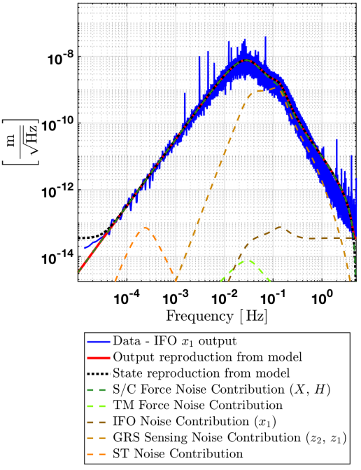
This plot is assuming a GRS $\displaystyle z$ sensing with a noise floor of $\displaystyle 1.8\ 10^{-9}$\displaystyle\mathrm{m}\text{\,}\mathrm{\text{}^{-1/2}}$$ and a $\displaystyle\nicefrac{{1}}{{f}}$ noise increase from $\displaystyle 1$\displaystyle\mathrm{mHz}$$ and below. The S/C force and torque noise levels, extracted from equation 4, are all measured to be consistent with white noise. The white noise level along the $\displaystyle X$ axis is measured to be of $\displaystyle 0.17$\displaystyle\mathrm{\SIUnitSymbolMicro N}\text{\,}\mathrm{\text{}^{-1/2}}$$. See section VI and table 2 for more details.

As an example, figure 2 shows the spectral density of the $\displaystyle o_{1}$ channel during the April 2016 run, i.e. the in-loop optical sensor read-out of the $\displaystyle x_{1}$ coordinate (cf. reference axes of figure 1). In the figure are traced together the observed data (in blue) and the sum of all the contributors (in red), as predicted by a state space model of the closed loop system Weyrich (2008) (cf. section V and equation 2). The remaining lines show the break-down of the different components that contribute significantly to the sum: the external, out-of-loop forces applied on the S/C and the GRS sensing noise (mostly $\displaystyle z_{1}$ and $\displaystyle z_{2}$ sensing noise as visible after breaking down the contribution further) which are superimposed. The S/C force noise curve (dark green) is essentially due to the micro-thruster noise, for movements along X and rotation around Y. This has been demonstrated by using the Colloidal and cold-gas micronewton thruster systems alternatively and jointly Anderson et al. (2018). Note that the presence of a strong GRS sensing noise component, around $\displaystyle 0.1$\displaystyle\mathrm{Hz}$$, is due to the control strategy. Further details about this model reconstruction, and other examples, are given in section V.

The residual spectrum of $\displaystyle o_{1}$ reflects the frequency behaviour of the drag-free control gain. Below $\displaystyle 0.1$\displaystyle\mathrm{Hz}$$, the control loop gain is high and counters the noisy forces applied on the S/C (mostly thruster noise but also solar noise, etc.).

The drag-free gains continuously decrease with increasing frequencies to reach a minimum around $\displaystyle 30$\displaystyle\mathrm{mHz}$$. The spectrum is conversely increasing as $\displaystyle f^{2}$, reaching its maximum jitter level of about $\displaystyle 7$\displaystyle\mathrm{nm}\text{\,}\mathrm{\text{}^{-1/2}}$$ around $\displaystyle 30$\displaystyle\mathrm{mHz}$$. At higher frequencies, the $\displaystyle{f^{-2}}$ behaviour, due to the inertia of the TMs, is responsible for the spectrum drop. On the right end of the plot, above $\displaystyle 1$\displaystyle\mathrm{Hz}$$, one would normally see read-out noise floor only. However, as shown by the dark brown dashed line on the right end of the plot, the optical sensing noise is outstandingly low, less than $\displaystyle 0.1$\displaystyle\mathrm{pm}\text{\,}\mathrm{\text{}^{-1/2}}$$ as already presented in Armano et al. (2016), such that it has almost no perceptible impact on $\displaystyle o_{1}$ in the frequency domain of interest. The discrepancy between the data (blue line) and the model prediction (thick red line) visible above $\displaystyle 0.5$\displaystyle\mathrm{Hz}$$ is considered to be due to the imperfection of the $\displaystyle SSM$ model which does not reflect the non linear nature of the micronewton thruster system (e.g. pure delays). This has been confirmed by a comparison with ESA’s simulator that does not assume this linear aspect.

The spectrum breakdown also gives interesting information about the Multiple-Input-Multiple-Output (MIMO) nature of the in-loop dynamics. In figure 2, this appears clearly with the superimposed light brown dashed lines that shows the influence of the GRS sensing noise on the spectrum of $\displaystyle x_{1}$, yet sensed by the OMS. Indeed, $\displaystyle z_{1}$ and $\displaystyle z_{2}$ sensing noise induces noisy S/C $\displaystyle Y$-axis ($\displaystyle\eta$) rotations as expected from the control scheme exposed in table 1. This motion causes an apparent $\displaystyle x-$axis displacement of the TM1 inside its housing, the projection depending on the geometrical position of the housing w.r.t. the centre of mass of the S/C. This effect competes with force noise on the S/C at high frequencies.

V.  Spectrum Decomposition Using a State Space Model of the System

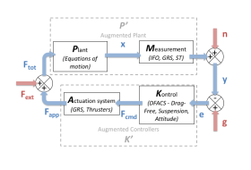
As shown in the previous section, breaking down the data according to a physical model turns out to be very informative for tracking down the physical origins of the in-loop coordinates spectral behaviour. This model developed by the LISA Pathfinder collaboration Weyrich (2008) (and implemented within the LTPDA software Hewitson et al. (2009)) is a Linear Time Invariant (LTI) State Space Model (SSM), meaning that the modeled dynamical behaviour of the closed loop system does not depend on time, nor on the actual dynamical state. The latter is encoded within a state-space representation in such a way that the $\displaystyle N_{th}$-order differential system governing the dynamics transforms into a matrix system of $\displaystyle N$ first-order equations, thus benefiting from the matrix algebra arsenal. The linearity and stationarity of the model allows for straightforward conversions between time-domain SSM and frequency domain transfer functions. The superposition principle holds because of linearity and allows one to decompose all the resulting spectra into their various contributions by extracting the relevant Single-Input-Single-Output (SISO) transfer functions from the MIMO model. In that spirit, the in-loop sensor outputs can be decomposed with the help of closed loop transfer functions called sensitivity functions, which encode the sensitivity of the outputs to various out-of-loop disturbance signals, such as the sensing noise or the force noise applied on the bodies. Their respective transfer functions are named the $\displaystyle S$-gain and the $\displaystyle L$-gain as typically seen in the literature, and are given by the expressions:

$$\displaystyle S(f)=\frac{1}{1+P^{\prime}K^{\prime}} \displaystyle L(f)=\frac{P^{\prime}}{1+P^{\prime}K^{\prime}}$$

$$\displaystyle T(f)=\frac{P^{\prime}K^{\prime}}{1+P^{\prime}K^{\prime}}$$ (1)

whereas $\displaystyle P$, standing for Plant, are the transfer functions of the dynamical system under DFACS control (forces/torques to displacements) and $\displaystyle K$ encodes the transfer functions of the DFACS. The prime symbols mention that these transfer functions are also including the transfer functions of the actuators ($\displaystyle K^{\prime}=KA$) and of the sensors ($\displaystyle P^{\prime}=MP$), for sake of notation simplification. Hence, these closed-loop transfer functions potentially depend on all the subsystem transfer functions involved in the control loop, and more significantly on the plant dynamics and the control laws. Figure 3 gives an illustration of LISA Pathfinder closed-loop system which shows explicitly these transfer functions and the various in-loop and out-of-loop variables. Mathematically, the spectrum breakdown can be expressed in the following way:

$$\tilde{Y}^{\scriptscriptstyle q}=\sum\limits_{\scriptscriptstyle p=x,y,z,\theta,\eta,\phi}L_{\scriptscriptstyle\text{gain}}^{\scriptscriptstyle qp}\tilde{F}_{\scriptscriptstyle\text{ext}}^{\scriptscriptstyle p}+\sum\limits_{\scriptscriptstyle p=x,y,z,\theta,\eta,\phi}S_{\scriptscriptstyle\text{gain}}^{\scriptscriptstyle qp}\tilde{n}^{\scriptscriptstyle p}$$ (2)

where $\displaystyle\tilde{Y}^{\scriptscriptstyle q}$, $\displaystyle\tilde{F}_{\scriptscriptstyle\text{ext}}^{\scriptscriptstyle p}$ and $\displaystyle\tilde{n}^{\scriptscriptstyle p}$ are the Fourier transforms, for the degree of freedom $\displaystyle q$, of the associated in-loop sensor output, the out-of-loop force noises and sensing noises LISA Pathfinder collaboration (2017) respectively. Because the $\displaystyle S$-gain (the sensitivity function) and the $\displaystyle L$-gain (load disturbance sensitivity function ) are both MIMO functions, a sum is performed over the extra dimension to account for cross-couplings effects that can have an important impact on the spectra (like the role played by GRS sensing noise on the spectra of the figure 2).

Figure 3: Simplified diagram of LISA Pathfinder closed loop system. The closed loop system is excited via three different out-of-loop signal channels: the guidance signal $\displaystyle g$ (null in the case of ”noise only run”), the sensing noise $\displaystyle n$, and the external forces $\displaystyle F_{ext}$. The in-loop variables are indicated in blue, whereas the out-of-loop signals are in red. The in-loop variables are successively the states of motion $\displaystyle X$, the observed displacements $\displaystyle Y$, the error signal compared to targeted displacements $\displaystyle e$, the commanded $\displaystyle F_{cmd}$ forces, the effectively applied forces $\displaystyle F_{app}$ and the total resulting forces $\displaystyle F_{tot}$.

A number of instances illustrate this type of decomposition. A case of particular interest is the spectra of the TMs angular displacements around $\displaystyle y$ and $\displaystyle z$ axes, which corresponding angles are labelled $\displaystyle\eta$ and $\displaystyle\phi$. The residuals behave in the most complex fashion because of numerous contributions that are equally competing to alter the TM orientation. As an example, figure 4 shows the spectral density of the in-loop $\displaystyle\eta_{1}$ optical sensing output. Every control type of the DFACS - drag-free, suspension and attitude controls - has an influence on this plot.

Figure 4: Decomposition of the in-loop DWS measurement $\displaystyle\eta_{1}$ spectrum into its various noise source contributions. The same explanations as in figure 2 apply.
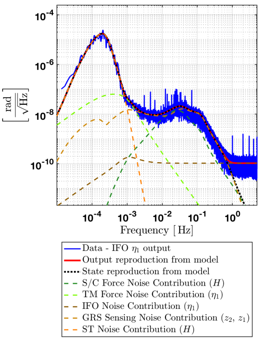
This plot is assuming: a Star Tracker sensing noise of $\displaystyle 3.7\ 10^{-4}$\displaystyle\mathrm{rad}\text{\,}\mathrm{\text{}^{-1/2}}$$ at $\displaystyle 0.2$\displaystyle\mathrm{mHz}$$, with a noise floor starting from $\displaystyle 5$\displaystyle\mathrm{mHz}$$ at a level of $\displaystyle 2.0\ 10^{-5}$\displaystyle\mathrm{rad}\text{\,}\mathrm{\text{}^{-1/2}}$$; a TM torque noise of $\displaystyle 7.1\ 10^{-16}$\displaystyle\mathrm{N}\text{\,}\mathrm{\text{}^{-1/2}}$$ across the whole bandwidth; a GRS $\displaystyle z$ sensing with a noise floor of $\displaystyle 1.8\ 10^{-9}$\displaystyle\mathrm{m}\text{\,}\mathrm{\text{}^{-1/2}}$$, a $\displaystyle\nicefrac{{1}}{{f}}$ noise increase from $\displaystyle 1$\displaystyle\mathrm{mHz}$$ and below, reaching a level of $\displaystyle 4.6\ 10^{-9}$\displaystyle\mathrm{m}\text{\,}\mathrm{\text{}^{-1/2}}$$ at $\displaystyle 0.1$\displaystyle\mathrm{mHz}$$; a S/C torque noise around its $\displaystyle Y$ axis of $\displaystyle 6.7\ 10^{-8}$\displaystyle\mathrm{N}\text{\,}\mathrm{m}\text{\,}\mathrm{\text{}^{-1/2}}$$; a white DWS $\displaystyle\eta$ noise of $\displaystyle 1.05\ 10^{-10}$\displaystyle\mathrm{rad}\text{\,}\mathrm{\text{}^{-1/2}}$$. See section VI and table 2 for more details.

At the highest frequencies, the $\displaystyle\eta_{1}$ DWS sensing noise (dashed dark brown line) is the dominant factor. From $\displaystyle 0.5$\displaystyle\mathrm{mHz}$$ to $\displaystyle 0.5$\displaystyle\mathrm{Hz}$$ there is a complex interplay between the external forces applied on the S/C (i.e. micronewton thrusters), residuals of the drag-free compensation, and the GRS sensing noise (light brown) of $\displaystyle y_{1}$, $\displaystyle y_{2}$ and $\displaystyle\theta_{1}$ that are all Drag-Free controlled. At the lowest frequencies, the Star Tacker noise (orange line) which acts through the Attitude Control is the dominant source. It should be noticed that some of these noise sources, such as GRS $\displaystyle y_{1}$ and $\displaystyle y_{2}$ sensing noise (light brown), can be measured more directly through other channels; for example, see the analysis done in figure 5. In the region around $\displaystyle 1$\displaystyle\mathrm{mHz}$$, in figure 4 back again, one is in presence of an ambiguity because observed spectrum can either be explained by the impact of TM torque noise of $\displaystyle\eta_{1}$ (light green) or by enhancing the reddening of the noise of $\displaystyle y_{1}$ and $\displaystyle y_{2}$ sensors. To remove this ambiguity, the reddening ($\displaystyle 1/f$ behaviour) has been measured independently by Armano et al. (2017).

Figure 5 shows the behaviour of the $\displaystyle z_{1}$ sensing output. This case is representative of what can also be observed for Drag-Free variables such as outputs $\displaystyle y_{1}$, $\displaystyle y_{2}$, $\displaystyle z_{2}$ and $\displaystyle\theta_{1}$. These spectra are much simpler than for the $\displaystyle\eta$ and $\displaystyle\phi$ channels. At the highest frequencies, the sensing noise (of $\displaystyle z_{1}$ in the figure) can be directly extracted. At lower frequencies, the behaviour of the spectra is essentially controlled by the $\displaystyle Z$ external forces exerted on the S/C, which means an estimation of this noise is also readily measurable.

Figure 5: Decomposition of the in-loop GRS measurement $\displaystyle z_{2}$ spectrum into its various noise source contributions. The same explanations as in figure 2 apply. Note that the $\displaystyle z_{2}$ state (black dashed line) - or $\displaystyle z_{2}$ ”true motion” - predicted from the model deviates very significantly from the in-loop GRS sensed $\displaystyle z_{2}$ displacement (data in blue, model in red). As discussed in detail at section VII, the GRS sensor noise induce a jitters of the S/C at low frequency (here $\displaystyle f<1$\displaystyle\mathrm{mHz}$$) which is not observable from the in-loop GRS $\displaystyle z_{2}$ output.
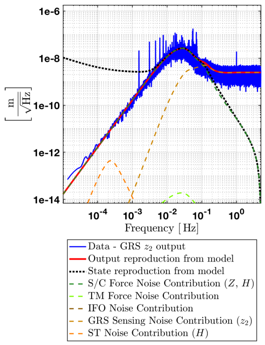
This plot is assuming a GRS $\displaystyle z$ sensing with a noise floor of $\displaystyle 1.5\ 10^{-9}$\displaystyle\mathrm{m}\text{\,}\mathrm{\text{}^{-1/2}}$$, a $\displaystyle\nicefrac{{1}}{{f}}$ noise increase from $\displaystyle 1$\displaystyle\mathrm{mHz}$$ and below, reaching a level of $\displaystyle 4.5\ 10^{-9}$\displaystyle\mathrm{m}\text{\,}\mathrm{\text{}^{-1/2}}$$ at $\displaystyle 0.1$\displaystyle\mathrm{mHz}$$. The S/C force and torque noise levels, extracted from equation 4, are all measured to be consistent with white noise. The white noise level along the $\displaystyle Z$ axis is measured to be of $\displaystyle 4.6\ 10^{-7}$\displaystyle\mathrm{N}\text{\,}\mathrm{\text{}^{-1/2}}$$. See section VI and table 2 for more details.

VI.  Sensing and Actuation Noise

In the above section, equation 2 shows how the out-of-loop force and sensing noises impact the observed spectra. In this section we begin by giving some illustrative examples of how the noise levels impact different frequency ranges and we then present our quantitative results in table 2. Depending on the frequency range, a given noise will dominate the observed spectra. For instance, at the highest frequencies (typically from $\displaystyle f>1$\displaystyle\mathrm{Hz}$$), observed displacements of the S/C and the TMs are nearly insensitive to input external forces. Indeed, referring to equation 2, $\displaystyle S_{\text{gain}}\approx 1$ and $\displaystyle L_{\text{gain}}\approx 0$ in such region, reflecting the fact the inertia of the bodies increases along with frequency, as a consequence of the $\displaystyle\nicefrac{{1}}{{f^{2}}}$ behavior of the dynamical system (double integrator, i.e. from force to displacement). Consequently, the noise of a given sensor dominates the observed spectra in most cases, allowing for a straightforward determination of its level: see the dashed brown lines in figures 4 or 5 as examples. An exception is showed by figure 2 where the sensor noise level is so low that even at the highest frequencies the sensitivity to the sensing noise is not reached and a determination of its noise level cannot be made. In reference Armano et al. (2018), the x1 IFO noise level is indeed shown to be as small as $\displaystyle 30$\displaystyle\mathrm{fm}\text{\,}\mathrm{\text{}^{-1/2}}$$. At lower frequencies, below $\displaystyle 5$\displaystyle\mathrm{mHz}$$, the out-of-loop S/C force noise usually dominates, see in figure 5 the dashed green line. The level of these noises can be determined with the help of the commanded forces or torques on/around the corresponding axis (see equation 3, discussed later in the section). In the case of figure 4 the situation is different and below $\displaystyle 1$\displaystyle\mathrm{mHz}$$ the Star Tracker noise dominates (brown dashed line). We discuss later in this section how these noises are estimated.

In most instances, the frequency dependence of the noises are not directly measurable by an analysis of the spectra, because they are here not distinguishable from that of the closed-loop model transfer function. We used therefore the results of independent and dedicated investigations that were performed during the mission. For the capacitive sensing noises, we refer to Armano et al. (2017) which showed that these noises had a $\displaystyle\nicefrac{{1}}{{\sqrt{f}}}$ (in amplitude) dependence below $\displaystyle 1$\displaystyle\mathrm{mHz}$$ whereas, for the capacitive actuation noises, LISA Pathfinder collaboration showed a $\displaystyle\nicefrac{{1}}{{f}}$ dependence (in amplitude) below $\displaystyle 1$\displaystyle\mathrm{mHz}$$. We have performed an analysis of all the observables ($\displaystyle x,\ y,\ z,\ \theta,\ \eta$ and $\displaystyle\phi$) associated to TM1 for a number of noise only runs. The results, obtained for April 2016 and January 2017, are collected in table 2. On the left panel of this table we list the sensing noises that we have used (see table 1 for more details about the degrees of freedom). The first six lines correspond to the linear and angular sensing noises of TM1, whereas the last three lines correspond to the S/C Star Tracker noise. The third and fourth columns gives the values obtained in April 2016 and January 2017. The right panel of the table gives the values for the actuation noises. The first 6 lines correspond to the out-of-loop forces and torques on the S/C whereas the last 5 lines correspond to the capacitive actuation forces on TM1. The values given in this table correspond to the noise level at high frequencies. The $\displaystyle 5th$ and $\displaystyle 9th$ columns give the corner frequency and the power of the reddening of the noise below the corner frequency, when applicable.

Two special cases have to be highlighted. The last three observables on the left panel of the table (Star Tracker noises, entries 7-9) are obtained from a fit to the spectrum of the attitude control error signals out of the DFACS, corrected by the S-gain of the corresponding control loop. The attitude control is effective at frequencies well below the measurement bandwidth and the star tracker noise level dominates any actual S/C rotations in the latter bandwidth, which means that the attitude control error signal provides a direct measurement of the attitude sensor noise essentially, as confirmed by the state space model of the closed-loop system. From these time series, a fit is obtained assuming a white noise at high frequencies, a rise for frequencies below $\displaystyle 3$\displaystyle\mathrm{mHz}$$ and a saturation below $\displaystyle 0.4$\displaystyle\mathrm{mHz}$$. The values given in table 2 correspond to the white noise floor. It should be noted that the Star Tracker noises also show a number of features, i.e. peaks in the frequency domain around $\displaystyle 5$\displaystyle\mathrm{mHz}$$, which are not included in the corresponding fits. With regards to the actuation noise on the right-hand panel of the table, the first six entries correspond to the noisy external forces and torques applied on the S/C, essentially by the thruster system itself (as discussed in section IV). This force noise can be measured from the calculation of the out-of-loop forces exerted on the S/C. Equations 3, 4 and 5 present such calculations, where the indices ool and cmd distinguish between out-of-loop forces and torques applied, and those commanded by the control loop (that oppose the ool forces and torques when the control gain is high). The meaning of the variables has been detailed in table 1. The mass terms $\displaystyle m_{\scriptscriptstyle\text{SC}}$, $\displaystyle m_{\scriptscriptstyle 1}$, $\displaystyle m_{\scriptscriptstyle 2}$, $\displaystyle I_{\scriptscriptstyle\text{SC}}$, $\displaystyle I_{\scriptscriptstyle 1}$ are the mass and the inertia matrices of the S/C and of the two TMs respectively (the TMs are labelled by their numbers only). Also, $\displaystyle d$ denotes the distance between the working points of the two TMs (namely the centres of their housings).

$$\vec{n}^{\scriptscriptstyle\text{\text{thruster}}}\approx\begin{bmatrix}&\vec{F}_{\scriptscriptstyle\text{SC}}^{\scriptscriptstyle\text{ool}}\\ &\vec{T}_{\scriptscriptstyle\text{SC}}^{\scriptscriptstyle\text{ool}}\end{bmatrix}\\$$ (3)

$$\displaystyle\vec{F}_{\scriptscriptstyle\text{SC}}^{\scriptscriptstyle\text{ool}}=m_{\scriptscriptstyle\text{SC}}\begin{bmatrix}&\ddot{o_{\scriptscriptstyle 1}}\\ &\frac{\ddot{z_{\scriptscriptstyle 1}}+\ddot{z_{\scriptscriptstyle 2}}}{2}\\ &\frac{\ddot{y_{\scriptscriptstyle 1}}+\ddot{y_{\scriptscriptstyle 2}}}{2}\end{bmatrix} \displaystyle-\vec{F}_{\scriptscriptstyle\text{SC}}^{\scriptscriptstyle\text{cmd}}$$ (4)

$$\displaystyle\vec{T}_{\scriptscriptstyle\text{SC}}^{\scriptscriptstyle\text{ool}}=I_{\scriptscriptstyle\text{SC}}\begin{bmatrix}&\ddot{\theta_{\scriptscriptstyle 1}}-\frac{T_{\scriptscriptstyle x1}}{I_{\scriptscriptstyle 1,xx}}\\ &\frac{\ddot{z_{\scriptscriptstyle 2}}-\ddot{z_{\scriptscriptstyle 1}}}{2d}-\big{(}\frac{F_{\scriptscriptstyle z2}}{m_{\scriptscriptstyle 2}}-\frac{F_{\scriptscriptstyle z1}}{m_{\scriptscriptstyle 1}}\big{)}\\ &\frac{\ddot{y_{\scriptscriptstyle 1}}-\ddot{y_{\scriptscriptstyle 2}}}{2d}-\big{(}\frac{F_{\scriptscriptstyle y1}}{m_{\scriptscriptstyle 1}}-\frac{F_{\scriptscriptstyle y2}}{m_{\scriptscriptstyle 2}}\big{)}\end{bmatrix} \displaystyle-\vec{T}_{\scriptscriptstyle\text{SC}}^{\scriptscriptstyle\text{cmd}}$$ (5)

The actuation noises of the capacitive actuators are addressed in the last five entries (7-11) on the right-hand side of the table. The force noise for linear degrees of freedom ($\displaystyle y$ and $\displaystyle z$) are estimated from extrapolation of the $\displaystyle x$ noise. They are built from the addition of the Brownian noise level observed for the $\displaystyle x$ channels Armano et al. (2016) and a model-based extrapolation of the actuation noise for degrees of freedom other than $\displaystyle x$, which is expected to be dominant below $\displaystyle 0.5$\displaystyle\mathrm{mHz}$$ because of the larger force and torque authorities along/around these axes. Regarding the torque noises (entries 9-10), their levels are measured at low frequency with the help of the following expression:

$$\displaystyle\vec{T}_{\scriptscriptstyle 1/2}^{\scriptscriptstyle\text{ool}}=\frac{I_{\scriptscriptstyle 1/2}}{\sqrt{2}}\begin{bmatrix}&-\\ &\big{(}\ddot{\eta_{\scriptscriptstyle 2}}-\ddot{\eta_{\scriptscriptstyle 1}}\big{)}-\Big{(}\frac{T_{\scriptscriptstyle y2}}{I_{\scriptscriptstyle 2,yy}}-\frac{T_{\scriptscriptstyle y1}}{I_{\scriptscriptstyle 1,yy}}\Big{)}\\ &\big{(}\ddot{\phi_{\scriptscriptstyle 2}}-\ddot{\phi_{\scriptscriptstyle 1}}\big{)}-\Big{(}\frac{T_{\scriptscriptstyle z2}}{I_{\scriptscriptstyle 2,zz}}-\frac{T_{\scriptscriptstyle z1}}{I_{\scriptscriptstyle 1,zz}}\Big{)}\end{bmatrix}$$ (6)

In equation 6, calculating the difference between IFO angular displacement measurements of the two TMs rejects common mode noise angular accelerations of the TMs, therefore the impact of S/C to TMs angular acceleration. Subtracting capacitive commanded torques provides then an estimate of the out-of-loop torques on the TMs. However, this calculation is typically valid only below $\displaystyle 1$\displaystyle\mathrm{mHz}$$, above which frequency sensing noise rapidly dominates. Below $\displaystyle 1$\displaystyle\mathrm{mHz}$$, applying 6 to the data, a flat noise torque is observed down to around $\displaystyle 0.01$\displaystyle\mathrm{mHz}$$. As a conservative assumption, this white noise torque is averaged and extrapolated to the whole frequency band (hence labelled as white noise in table 2). Note that equation 6 is not applicable to linear degrees of freedom $\displaystyle y$ and $\displaystyle z$, since their differential channels are essentially sensitive to the largely dominant S/C angular acceleration noise and are Drag-Free controlled. A similar limitation applies to the $\displaystyle\theta$ case.

In table 2, comparison between April 2016 and January 2017 data sets allows to appreciate the consistency between the ”noise runs” and the stationnarity of the sensor and actuator performances. It is worth mentioning that independent studies by Anderson et al. (2018) also show consistent results and similar performances for the cold-gas thrusters at different times of the mission (September 2016 and April 2017).

Table 2: Table of sensing and actuation noises. $\displaystyle N.S$ stands for ”Not Sensitive” and ST for Star Tracker. $\displaystyle W.N$. stands for white noise. See the text for further explanations.

#	Sensing Noise	Apr. 2016	Jan. 2017	$\displaystyle f_{c}:\alpha$	Actuation Noise	Apr. 2016	Jan. 2017	$\displaystyle f_{c}:\alpha$
1	$\displaystyle o_{1}\ ($\displaystyle\mathrm{m}\text{\,}\mathrm{\text{}^{-1/2}}$)$	$\displaystyle 35.0\ 10^{-15}$	$\displaystyle N.S$	$\displaystyle N.S$	$\displaystyle Ext.\ X\ ($\displaystyle\mathrm{N}\text{\,}\mathrm{\text{}^{-1/2}}$)$	$\displaystyle 1.7\ 10^{-7}$	$\displaystyle 1.9\ 10^{-7}$	$\displaystyle W.N.$
2	$\displaystyle y_{1}\ ($\displaystyle\mathrm{m}\text{\,}\mathrm{\text{}^{-1/2}}$)$	$\displaystyle 1.5\ 10^{-9}$	$\displaystyle 1.5\ 10^{-9}$	$\displaystyle\hskip 2.84526pt1$\displaystyle\mathrm{mHz}$:-0.5\hskip 2.84526pt$	$\displaystyle Ext.\ Y\ ($\displaystyle\mathrm{N}\text{\,}\mathrm{\text{}^{-1/2}}$)$	$\displaystyle 1.4\ 10^{-7}$	$\displaystyle 1.7\ 10^{-7}$	$\displaystyle W.N.$
3	$\displaystyle z_{1}\ ($\displaystyle\mathrm{m}\text{\,}\mathrm{\text{}^{-1/2}}$)$	$\displaystyle 1.8\ 10^{-9}$	$\displaystyle 1.7\ 10^{-9}$	$\displaystyle 1$\displaystyle\mathrm{mHz}$:-0.5$	$\displaystyle Ext.\ Z\ ($\displaystyle\mathrm{N}\text{\,}\mathrm{\text{}^{-1/2}}$)$	$\displaystyle 4.6\ 10^{-7}$	$\displaystyle 3.3\ 10^{-7}$	$\displaystyle W.N.$
4	$\displaystyle\theta_{1}\ ($\displaystyle\mathrm{rad}\text{\,}\mathrm{\text{}^{-1/2}}$)$	$\displaystyle 9.4\ 10^{-8}$	$\displaystyle 1.1\ 10^{-7}$	$\displaystyle 1$\displaystyle\mathrm{mHz}$:-0.5$	$\displaystyle Ext.\ \theta\ ($\displaystyle\mathrm{N}\text{\,}\mathrm{m}\text{\,}\mathrm{\text{}^{-1/2}}$)$	$\displaystyle 9.8\ 10^{-8}$	$\displaystyle 7.5\ 10^{-8}$	$\displaystyle W.N.$
5	$\displaystyle\eta_{1}\ ($\displaystyle\mathrm{rad}\text{\,}\mathrm{\text{}^{-1/2}}$)$	$\displaystyle 1.05\ 10^{-10}$	$\displaystyle 1.06\ 10^{-10}$	$\displaystyle 1$\displaystyle\mathrm{mHz}$:-0.5$	$\displaystyle Ext.\ \eta\ ($\displaystyle\mathrm{N}\text{\,}\mathrm{m}\text{\,}\mathrm{\text{}^{-1/2}}$)$	$\displaystyle 6.7\ 10^{-8}$	$\displaystyle 7.8\ 10^{-8}$	$\displaystyle W.N.$
6	$\displaystyle\phi_{1}\ ($\displaystyle\mathrm{rad}\text{\,}\mathrm{\text{}^{-1/2}}$)$	$\displaystyle 2.05\ 10^{-10}$	$\displaystyle 2.05\ 10^{-10}$	$\displaystyle 1$\displaystyle\mathrm{mHz}$:-0.5$	$\displaystyle Ext.\ \phi\ ($\displaystyle\mathrm{N}\text{\,}\mathrm{m}\text{\,}\mathrm{\text{}^{-1/2}}$)$	$\displaystyle 1.7\ 10^{-7}$	$\displaystyle 1.9\ 10^{-7}$	$\displaystyle W.N.$
7	ST $\displaystyle\theta\ ($\displaystyle\mathrm{rad}\text{\,}\mathrm{\text{}^{-1/2}}$)$	$\displaystyle 2.1\ 10^{-6}$	$\displaystyle 2.1\ 10^{-6}$	see text	$\displaystyle Fy_{1}\ ($\displaystyle\mathrm{N}\text{\,}\mathrm{\text{}^{-1/2}}$)$	$\displaystyle 8.0\ 10^{-15}$		$\displaystyle 1$\displaystyle\mathrm{mHz}$:-1$
8	ST $\displaystyle\eta\ ($\displaystyle\mathrm{rad}\text{\,}\mathrm{\text{}^{-1/2}}$)$	$\displaystyle 2.0\ 10^{-5}$	$\displaystyle 2.0\ 10^{-5}$	see text	$\displaystyle Fz_{1}\ ($\displaystyle\mathrm{N}\text{\,}\mathrm{\text{}^{-1/2}}$)$	$\displaystyle 8.0\ 10^{-15}$		$\displaystyle 1$\displaystyle\mathrm{mHz}$:-1$
9	ST $\displaystyle\phi\ ($\displaystyle\mathrm{rad}\text{\,}\mathrm{\text{}^{-1/2}}$)$	$\displaystyle 3.2\ 10^{-6}$	$\displaystyle 3.2\ 10^{-6}$	see text	$\displaystyle Ty_{1}\ ($\displaystyle\mathrm{N}\text{\,}\mathrm{m}\text{\,}\mathrm{\text{}^{-1/2}}$)$	$\displaystyle 7.1\ 10^{-16}$	$\displaystyle 7.4\ 10^{-16}$	W.N.
10					$\displaystyle Tz_{1}\ ($\displaystyle\mathrm{N}\text{\,}\mathrm{m}\text{\,}\mathrm{\text{}^{-1/2}}$)$	$\displaystyle 2.6\ 10^{-16}$	$\displaystyle 1.9\ 10^{-16}$	W.N.

VII.  The Stability of the Spacecraft

It has been shown in the previous sections that the SSM was able to reproduce and explain the in-loop observations of the linear and angular displacements of the TMs relative to the S/C through breaking down the control residuals into the respective contributions of the individual noise sources. This model can now be used to assess physical quantities that are out of reach of on-board sensors, such as ”true displacement” of the bodies and their acceleration w.r.t. their local inertial frame.

Indeed, using properties of the Space State Model, one can extract the true movement of the S/C with respect to the TMs. This is done using the following formula:

$$\tilde{\textbf{X}}_{\scriptscriptstyle\text{SC}}^{\scriptscriptstyle q}=\sum\limits_{\scriptscriptstyle p=x,y,z,\theta,\eta,\phi}L_{\scriptscriptstyle\text{gain}}^{\scriptscriptstyle qp}\tilde{F}_{\scriptscriptstyle\text{ext}}^{\scriptscriptstyle p}+\sum\limits_{\scriptscriptstyle p=x,y,z,\theta,\eta,\phi}T_{\scriptscriptstyle\text{gain}}^{\scriptscriptstyle qp}\tilde{n}^{\scriptscriptstyle p}$$ (7)

where $\displaystyle\tilde{\textbf{X}}_{\scriptscriptstyle\text{SC}}^{\scriptscriptstyle q}$ is the Fourier transform, for the degree of freedom $\displaystyle q$, of the associated state variable, or alternatively called the true displacement (i.e, not the observed displacement) of the TMs with respect to the S/C. $\displaystyle T_{\scriptscriptstyle\text{gain}}^{\scriptscriptstyle qp}$ is commonly named the $\displaystyle T\ gain$, or the complementary sensitivity function LISA Pathfinder collaboration (2017). The difference between the true displacement and the observed displacement is that the former is estimated without applying the sensing noise whereas the latter corresponds to the response of the sensor output, i.e. with its noise. It should be noted, however, that the noise of previous time steps have an impact on the true displacement.

This important distinction is a classical feature of in-loop variables of feedback systems. A closed-loop system will force the variable of interest to its assigned guidance value, generally zero. To do this, for example, it will apply a correcting force to the S/C that will not only compensate for any external disturbances, but will also be triggered by the noise of the corresponding position sensor, indistinguishable from true motion from the point of view of the DFACS. As a result, when the sensing noise is the leading component, the compensating force will make the S/C jitter in the aim of canceling out the observed sensing noise. Hence the state variable will exhibit this movement whereas the sensor will show a value tending to its guidance at low frequency. Figure 8, discussed further in the text, illustrates this for the $\displaystyle Z$ axis acceleration.

Assuming TM1 follows a perfect geodesic, and following LPF’s DFACS philosophy (see table 1), the stability of the S/C is defined by the dynamic variables shown in equation 8:

$$\displaystyle\ddot{X}_{\scriptscriptstyle\text{SC}}=\ddot{x}_{\scriptscriptstyle 1} \displaystyle\ddot{\Theta}_{\scriptscriptstyle\text{SC}}=\ddot{\theta}_{\scriptscriptstyle 1}$$

$$\displaystyle\ddot{Y}_{\scriptscriptstyle\text{SC}}=\frac{\ddot{y}_{\scriptscriptstyle 1}+\ddot{y}_{\scriptscriptstyle 2}}{2} \displaystyle\ddot{H}_{\scriptscriptstyle\text{SC}}=\frac{\ddot{z}_{\scriptscriptstyle 2}-\ddot{z}_{\scriptscriptstyle 1}}{d}$$

$$\displaystyle\ddot{Z}_{\scriptscriptstyle\text{SC}}=\frac{\ddot{z}_{\scriptscriptstyle 1}+\ddot{z}_{\scriptscriptstyle 2}}{2} \displaystyle\ddot{\Phi}_{\scriptscriptstyle\text{SC}}=\frac{\ddot{y}_{\scriptscriptstyle 2}-\ddot{y}_{\scriptscriptstyle 1}}{d}$$ (8)

where $\displaystyle d$ is the distance between the two TMs.

However, the TMs cannot embody perfect local inertial frames, as they inevitably experience some stray forces, though of very low amplitude as previously demonstrated in Armano et al. (2016). Hence, as a second step, it is necessary to draw an estimation of the TMs acceleration w.r.t. their local inertial frames, and add it up to the relative acceleration between the TMs and the S/C calculated at the previous step. Reference Armano et al. (2016) provides the acceleration noise floor due to brownian noise ($\displaystyle S_{0}^{1/2}=5.6$\displaystyle\mathrm{fm}\text{\,}{\mathrm{s}}^{-2}\text{\,}\mathrm{\text{}^{-1/2}}$$, divided by $\displaystyle\sqrt{2}$ for the acceleration of a single TM), to which is added, in accordance to Armano et al. (2018), a $\displaystyle 1/f$ component starting from around $\displaystyle 0.5$\displaystyle\mathrm{mHz}$$ and below. The nature of this noise is still unknown to this day, but has to be included in the analysis nevertheless.

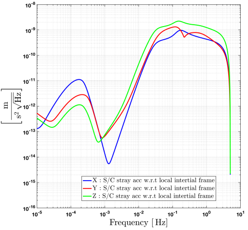
Another factor that impacts the LPF stability is the GRS actuation noise. On the X axis, the impact is minimal because the actuation authority is set to a minimal value, just above the one required to compensate for the internal gravity gradient. On the other axes and on the angular degrees of freedom however, the actuation noise is expected to be dominant below $\displaystyle 1$\displaystyle\mathrm{mHz}$$ according to model extrapolations for higher authority degrees of freedom LISA Pathfinder collaboration (see table 2 and discussion in section VI). Figures 6 and 7 show the stability (jitter) of the S/C and give a quantitative estimate of the true movement of the S/C (for linear and angular degrees of freedom, respectively) relative to the local geodesic. In these figures at high frequencies ($\displaystyle f\geqslant 2$\displaystyle\mathrm{Hz}$$), one can note because of inertia of the S/C, the stability of the S/C improves with frequency. The region between $\displaystyle 0.02$\displaystyle\mathrm{Hz}$$ and $\displaystyle 2$\displaystyle\mathrm{Hz}$$ is explained by the characteristics of the control loop which incompletely compensate the noise of the micronewton thruster system. Below this frequency band, the accelerations are exponentially suppressed by the drag free loop until the effects of the capacitive sensing devices are observed, see for example around $\displaystyle 2$\displaystyle\mathrm{mHz}$$ for the Y and Z accelerations in figure 6. Note that this effect is not observed on the X axis because the optical sensing device has a very low noise, of the order of $\displaystyle 35$\displaystyle\mathrm{fm}\text{\,}\mathrm{\text{}^{-1/2}}$$. Below $\displaystyle 1$\displaystyle\mathrm{mHz}$$ the noise coming from the Star Tracker and the unexplained $\displaystyle 1/f$ noise component explains the degradation of performance.

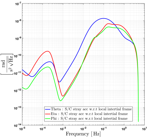
In figure 7, for $\displaystyle 1$\displaystyle\mathrm{mHz}$\leqslant f\leqslant 0.1$\displaystyle\mathrm{Hz}$$, one notices that $\displaystyle H$ and $\displaystyle\Phi$ stability are better that the one observed for $\displaystyle\theta$. This is because $\displaystyle\theta$ is measured by electrostatic angular sensor of TM1, whereas $\displaystyle\eta$ and $\displaystyle\phi$ are measured by combinations of $\displaystyle z_{1}$ and $\displaystyle z_{2}$ and of $\displaystyle y_{1}$ and $\displaystyle y_{2}$ (see table 1), which have higher SNR benefiting from a larger lever arm between electrodes and noise averaging from electrodes redundancy compared to the single GRS angular channel.

Figure 6: Stability of the S/C along X, Y and Z and as a function of frequency as simulated by the $\displaystyle LPF\ State\ Space\ Model$ using the parameters obtained from the April 2016 ”noise only run”.

Figure 7: Stability of the S/C along $\displaystyle\theta$, $\displaystyle\eta$ and $\displaystyle\phi$ and as a function of frequency as simulated by the $\displaystyle LPF\ State\ Space\ Model$ using the parameters obtained from the April 2016 ”noise only run”.

VIII.  Decomposing the Stability of the Spacecraft

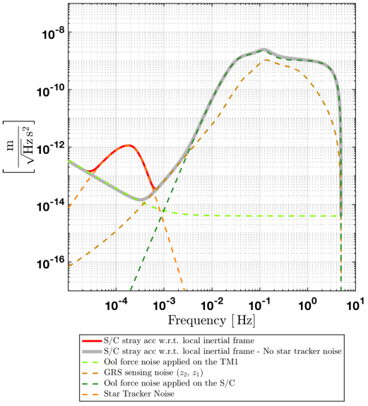
Figures 6 and 7 present the stability of the S/C on all degrees of freedom. They show the complex behaviour of these stability performances. It is important to understand where the observed features come from. As an example, figure 8 illustrates the decomposition of the acceleration stability on the $\displaystyle Z$ axis. Note that the $\displaystyle Z$ stability for LISA Pathfinder is calculated as the average $\displaystyle z$ values of TM1 and of TM2 (see equation 8). The red curve shows the sum of the listed contributions predicted by the State Space Model.

At the highest frequencies ($\displaystyle f\ >\ 0.5$\displaystyle\mathrm{Hz}$$) the $\displaystyle Z$ sensing noise and the out of loop noise (i.e. mainly thruster noises) are predominant contributors. They are however countered by the inertia of the heavy S/C that does not allow it to move significantly, hence the roll-off of the red curve up to the Nyquist frequency at $\displaystyle f=5$\displaystyle\mathrm{Hz}$$ for this data. At lower frequencies ($\displaystyle 5\ $\displaystyle\mathrm{mHz}$\ <\ f\ <\ 0.5\ $\displaystyle\mathrm{Hz}$$) , the out of loop forces are attenuated by the control loops, hence the exponential decrease below $\displaystyle 10$\displaystyle\mathrm{mHz}$$. Between $\displaystyle 0.5$\displaystyle\mathrm{mHz}$$ and $\displaystyle 5$\displaystyle\mathrm{mHz}$$, the GRS sensing noise on $\displaystyle Z$ is the dominant factor. This creates a movement of the S/C because the closed-loop system erroneously interprets this sensing noise as a non-zero position of the TMs to be corrected by the displacement of the S/C. Below this range the Star Tracker noise dominates, while at the lowest frequencies, the capacitive actuation noise governs the platform stability. Also indicated in this figure, and for illustration, is the effect of the Brownian noise which does not impact the stability performances on the $\displaystyle Z$ axis.

These explanations can be applied to all degrees of freedom with some differences for the $\displaystyle X$ axis. For this axis, the optical sensing noise is much smaller than GRS sensing noise and thus does not impact significantly the frequencies between $\displaystyle 0.5$\displaystyle\mathrm{mHz}$$ and $\displaystyle 5$\displaystyle\mathrm{mHz}$$. Another difference relates to the noise of capacitive actuation which is also much lower on X. At the lowest frequencies (around $\displaystyle 0.01$\displaystyle\mathrm{mHz}$$), one observes the impact of the ”excess noise” that is discussed in Armano et al. (2018).

Figure 8: Decomposition of the stability of the S/C along the $\displaystyle Z$ axis as a function of frequency. The red lines shows the SSM prediction and the other lines the contribution to this. The main contributors are the TMs force noise (light green dashed line), the star tracker noise (orange dashed line), the GRS sensing noise (light brown dashed lines) and the micro-thruster noise (dark green dashed line). See the text for further explanation.

IX.  The Impact of the Star Tracker Noise

Most of the contributions to S/C acceleration w.r.t. the local inertial observer are readily understandable. However, the impact of the Star Tracker noise is more subtle and needs explanation. The reason it impacts the platform stability is because the center of mass of the S/C does not coincide with the middle of the TM housing positions. By construction the center of mass is situated $\displaystyle 6.25$\displaystyle\mathrm{cm}$$ below the housings along Z axis, but due to mechanical imperfections, it is also offset by a few millimeters on the X and Y axis (see equation 9 and figure 9).

$$\displaystyle\overrightarrow{BH_{\scriptscriptstyle 1}}=\begin{bmatrix}0.183\\ -0.006\\ 0.0625\end{bmatrix}$\displaystyle\mathrm{m}$ \displaystyle\overrightarrow{BH_{\scriptscriptstyle 2}}=\begin{bmatrix}-0.193\\ -0.006\\ 0.0625\end{bmatrix}$\displaystyle\mathrm{m}$$$ (9)

Because of this, S/C rotation jitter driven by the noisy star tracker sensor induces an apparent linear displacement of the TMs inside their housings. Such linear displacement has a significant component along X if the center of mass happens to be off-centered w.r.t. the middle of the line joining the two TMs. The projection of the force on X indeed scales with the sine of the angle $\displaystyle\epsilon$ made by the line joining the center of the housing and the S/C center of mass (that is to say the vector $\displaystyle\vec{BH_{\scriptscriptstyle 1}}$), and the axis joining the two housings (the vector $\displaystyle\vec{H_{\scriptscriptstyle 1}H_{\scriptscriptstyle 2}}$). Such an effect can more formally be interpreted as the result of the (so-called) Euler force, an inertial force proportional to S/C angular acceleration arising from the point of view of a non-inertial platform. Consequently, the Drag-Free control will react on and correct the (so-induced) displacement of TM1 inside its housing. What was only an apparent force applied on the test mass then becomes a true force applied on the S/C along X through the micronewton thrusters and the feedback control. In fact, everything happens as though there existed a rotation-to-translation coupling of the S/C displacement, due to S/C geometry and DFACS activity. It is also worth noting that the impact on X-axis stability is observed to be greatly reduced in the case where the center of mass lies in the line joining TM housing centers.

Equation 10 provides an expression for the inertial forces responsible for the TMs displacement and equation 11 shows the Drag-Free control forces commanded to the micro-propulsion system in order to correct for the effect of the inertial forces. In these two equations, only the linear accelerations of the S/C are considered to emphasize the rotation-to-translation coupling of the S/C dynamics.

$$\displaystyle\vec{a}^{\scriptscriptstyle\text{ST}}=\begin{bmatrix}a_{\scriptscriptstyle x}^{\scriptscriptstyle\text{ST}}\\ a_{\scriptscriptstyle y}^{\scriptscriptstyle\text{ST}}\\ a_{\scriptscriptstyle z}^{\scriptscriptstyle\text{ST}}\end{bmatrix}=\begin{bmatrix}\Big{[}\dot{\vec{\omega}}\times\overrightarrow{BH_{\scriptscriptstyle 1}}\Big{]}\cdot\hat{X}\\ \nicefrac{{1}}{{2}}\Big{[}\dot{\vec{\omega}}\times(\overrightarrow{BH_{\scriptscriptstyle 1}}+\overrightarrow{BH_{\scriptscriptstyle 2}})\Big{]}\cdot\hat{Y}\\ \nicefrac{{1}}{{2}}\Big{[}\dot{\vec{\omega}}\times(\overrightarrow{BH_{\scriptscriptstyle 1}}+\overrightarrow{BH_{\scriptscriptstyle 2}})\Big{]}\cdot\hat{Z}\end{bmatrix}$$ (10)

$$\displaystyle\vec{F}_{\scriptscriptstyle\text{DF}}^{\scriptscriptstyle\text{ST}}=\begin{bmatrix}F_{\scriptscriptstyle\text{\text{DF, }}x}^{\scriptscriptstyle\text{ST}}\\ F_{\scriptscriptstyle\text{DF, }y}^{\scriptscriptstyle\text{ST}}\\ F_{\scriptscriptstyle\text{DF, }z}^{\scriptscriptstyle\text{ST}}\end{bmatrix}=-m_{\scriptscriptstyle S/C}\begin{bmatrix}a_{\scriptscriptstyle x}^{\scriptscriptstyle\text{ST}}\\ a_{\scriptscriptstyle y}^{\scriptscriptstyle\text{ST}}\\ a_{\scriptscriptstyle z}^{\scriptscriptstyle\text{ST}}\end{bmatrix}$$ (11)

Figure 9: Simplified sketch of LISA Pathfinder apparatus. The $\displaystyle xBz$ cross-section is represented here. The figure shows how any rotation of the S/C, in particular an $\displaystyle H$-rotation around the $\displaystyle Y$ axis, leads to apparent displacement of TM1 inside its housing that has a significant component along the $\displaystyle X$-axis (proportional to $\displaystyle\sin{\epsilon}$ here) when the S/C center of mass is shifted from the center of the two housings.

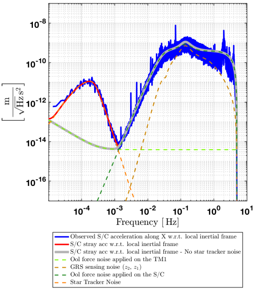
The State Space Model predicts such indirect influence of the star tracker if set with a center of mass located off the axis joining the two TMs. The set values in the model are the ones shown in the equation 9. Figure 10 shows the impact of the star tracker noise on the S/C stability along the X axis, together with all the other contributors already discussed in section VIII. The blue trace is the combination of data sensor outputs given by equations 12 and 13, and involving the double derivative of TM1 interferometer readout $\displaystyle\ddot{o}_{\scriptscriptstyle 1}$ and the measurement of the force applied to the S/C along X to counteract the Euler force, presented in equation 11. The angular acceleration of the satellite needed to compute the Euler force amplitude is recovered from GRS $\displaystyle\theta_{\scriptscriptstyle 1}$ measurements, and $\displaystyle z$ and $\displaystyle y$ differential measurements differentiated twice and corrected from the direct electrostatic actuation applied on the TMs $\displaystyle T_{\scriptscriptstyle X}^{\scriptscriptstyle\text{cmd}}$, $\displaystyle F_{\scriptscriptstyle z}^{\scriptscriptstyle\text{cmd}}$, $\displaystyle F_{\scriptscriptstyle y}^{\scriptscriptstyle\text{cmd}}$ in order to trigger the S/C rotation according to the DFACS control scheme (see table 1).

Figure 10 shows solid agreement between SSM predictions and computations from observations for the star tracker noise influence on stability along the X axis. It is visible in this figure that the star tracker noise deteriorated significantly platform stability at low frequencies by up to $\displaystyle 3$ orders of magnitude at $\displaystyle 0.1$\displaystyle\mathrm{mHz}$$. It is particularly noteworthy along the $\displaystyle X$ axis where high sensitivity of the optical sensor should have allowed for stability of the platform at the same level of quietness as the test mass itself (see the dark green dashed line in figure 10), if it was not for the presence of a noisy sensor such as the star tracker (relatively to the other sensors of very high performance) within the DFACS loop. It is also worth noting that such stability performance decrease due to S/C attitude sensing noise will be largely mitigated in the case of LISA, where Differential Wave-front Sensing of the inter-spacecraft laser link will provide attitude measurement of much higher precision. Figure 10 shows a projection to LISA performances (light gray) following this consideration, hence excluding the contribution from the star tracker noise. Besides, in the case of LISA, studying the stability of the S/C center of mass is less relevant than studying the stability of the optical benches, which are geometrically much closer to the TMs, and thus less affected by the rotation-to-translation coupling here discussed.

$$a_{\scriptscriptstyle X}^{\scriptscriptstyle\text{S/C, meas}}=-\ddot{o}_{\scriptscriptstyle 1}+\Big{[}\dot{\vec{\omega}}^{\scriptscriptstyle\text{meas}}\times\vec{BH_{\scriptscriptstyle 1}}\Big{]}\cdot\hat{X}$$ (12)

$$\displaystyle\dot{\vec{\omega}}^{\scriptscriptstyle\text{meas}}=\begin{bmatrix}\dfrac{T_{\scriptscriptstyle X}^{\scriptscriptstyle\text{cmd}}}{I_{\scriptscriptstyle XX}}-\ddot{\theta_{\scriptscriptstyle 1}}\\ \dfrac{\nicefrac{{F_{\scriptscriptstyle z2}^{\scriptscriptstyle\text{cmd}}}}{{m_{\scriptscriptstyle 2}}}-\nicefrac{{F_{\scriptscriptstyle z1}^{\scriptscriptstyle\text{cmd}}}}{{m_{\scriptscriptstyle 1}}}}{H_{\scriptscriptstyle 1}H_{\scriptscriptstyle 2}}-\dfrac{\big{(}\ddot{z_{\scriptscriptstyle 2}}-\ddot{z_{\scriptscriptstyle 1}}\big{)}}{H_{\scriptscriptstyle 1}H_{\scriptscriptstyle 2}}\\ \dfrac{\nicefrac{{F_{\scriptscriptstyle y2}^{\scriptscriptstyle\text{cmd}}}}{{m_{\scriptscriptstyle 2}}}-\nicefrac{{F_{\scriptscriptstyle y1}^{\scriptscriptstyle\text{cmd}}}}{{m_{\scriptscriptstyle 1}}}}{H_{\scriptscriptstyle 1}H_{\scriptscriptstyle 2}}-\dfrac{\big{(}\ddot{y_{\scriptscriptstyle 2}}-\ddot{y_{\scriptscriptstyle 1}}\big{)}}{H_{\scriptscriptstyle 1}H_{\scriptscriptstyle 2}}\end{bmatrix}$$ (13)

Figure 10: Stability of the S/C along $\displaystyle X$ as a function of frequency as simulated by the $\displaystyle LPF\ State\ Space\ Model$ (red) and as measured with a combination of observed data (blue) that takes into account the impact of the star tracker noise (according to equations 10 and 11). Similar to the red line, the gray solid trace gives the model prediction for X stability of the S/C, though excluding the impact of the star tracker, hence providing a projection to the LISA observatory case (for which attitude control will be driven by DWS sensing of the inter-spacecraft laser beam, seen as an inertial attitude reference). The dashed-line traces show the model decomposition. This figure uses parameters and data obtained from the April 2016 ”noise only run”.

X.  Conclusion

A frequency domain analysis and a decomposition of all in-loop coordinates associated to TM1 has been presented in order to highlight the DFACS performance of the LISA Pathfinder mission. The stability of the LISA Pathfinder platform, with respect to a local geodesic, has also been estimated.

A number of points can be concluded from this study:

• The study has shown that the LISA Pathfinder platform has remarkable performance in terms of stability over all degrees of freedom. The privileged $\displaystyle X$ axis has outstanding performance but the other degrees of freedom show adequate performance which demonstrate the interest of such a platform for other applications. Improvements in some of the sensors and actuators could enhance this performance.

• This study shows that the stability of LISA Pathfinder, in term of acceleration w.r.t local inertial reference frame, is sensitive to the GRS sensing noise around $\displaystyle 1$\displaystyle\mathrm{mHz}$$ and to TMs force noise at lower frequency. Above $\displaystyle 0.1$\displaystyle\mathrm{Hz}$$, the stability performances are impacted by the (micro-thruster) force noise and by the DFACS control loop.

• Below $\displaystyle 1$\displaystyle\mathrm{mHz}$$, the noise of the Star Tracker strongly impacts the performance of the system on all degrees of freedom. It should be noted however that, for LISA, several orders of magnitude improvements on attitude control performances are expected, benefiting from $\displaystyle\leavevmode\nobreak\ 10^{-8}$\displaystyle\mathrm{rad}\text{\,}\mathrm{\text{}^{-1/2}}$$ precision attitude sensing with DWS on the incoming long-range laser beam Amaro-Seoane et al. (2017), rather than the ($\displaystyle\leavevmode\nobreak\ 10^{-4}$\displaystyle\mathrm{rad}\text{\,}\mathrm{\text{}^{-1/2}}$$) level achieved by the LPF star tracker at low frequency, around $\displaystyle 0.1$\displaystyle\mathrm{mHz}$$.

• The LPF SSM Weyrich (2008) developed by the collaboration provides a reliable description of the closed loop dynamics, showing that the LISA Pathfinder system can be approximated by a linear system for frequencies lower than $\displaystyle 0.2Hz$. Hence, the State Space Model has been used to estimate the stability of the LISA Pathfinder platform over a wide frequency range, highlighting its remarkable performances.

• The demonstrated reliability of the model is an item of interest for the upcoming task of extrapolating LISA Pathfinder results towards LISA simulations and design. Such work is ongoing and will be published in the near future.

• The quality of the performances obtained by the LISA Pathfinder platform, with respect to the local geodesic, should therefore allow definition of similar platforms for other type of space-based measurements.

XI.   Acknowledgement

This work has been made possible by the LISA Pathfinder mission, which is part of the space-science programme of the European Space Agency.

The French contribution has been supported by the CNES (Accord Specific de projet CNES 1316634/CNRS 103747), the CNRS, the Observatoire de Paris and the University Paris-Diderot. E. Plagnol and H. Inchauspé would also like to acknowledge the financial support of the UnivEarthS Labex program at Sorbonne Paris Cité (ANR-10-LABX-0023 and ANR-11-IDEX-0005-02).

The Albert-Einstein-Institut acknowledges the support of the German Space Agency, DLR. The work is supported by the Federal Ministry for Economic Affairs and Energy based on a resolution of the German Bundestag (FKZ 50OQ0501 and FKZ 50OQ1601).

The Italian contribution has been supported by Agenzia Spaziale Italiana and Istituto Nazionale di Fisica Nucleare.

The Spanish contribution has been supported by contracts AYA2010-15709 (MICINN), ESP2013-47637-P, and ESP2015-67234-P (MINECO). M. Nofrarias acknowledges support from Fundacion General CSIC (Programa ComFuturo). F. Rivas acknowledges an FPI contract (MINECO).

The Swiss contribution acknowledges the support of the Swiss Space Office (SSO) via the PRODEX Programme of ESA. L. Ferraioli is supported by the Swiss National Science Foundation.

The UK groups wish to acknowledge support from the United Kingdom Space Agency (UKSA), the University of Glasgow, the University of Birmingham, Imperial College, and the Scottish Universities Physics Alliance (SUPA).

J. I. Thorpe and J. Slutsky acknowledge the support of the US National Aeronautics and Space Administration (NASA).

References

- Anza et al. (2005) S. Anza, M. Armano, E. Balaguer, M. Benedetti, C. Boatella, P. Bosetti, D. Bortoluzzi, N. Brandt, C. Braxmaier, M Caldwell, L. Carbone, A. Cavalleri, A. Ciccolella, I. Cristofolini, M. Cruise, M. D. Lio, K. Danzmann, D Desiderio, R. Dolesi, N. Dunbar, W. Fichter, C. Garcia, E. Garcia-Berro, A. F. G. Marin, R. Gerndt, A. Gianolio, D Giardini, R. Gruenagel, A. Hammesfahr, G. Heinzel, J. Hough, D. Hoyland, M. Hueller, O. Jennrich, U. Johann, S Kemble, C. Killow, D. Kolbe, M. Landgraf, A. Lobo, V. Lorizzo, D. Mance, K. Middleton, F. Nappo, M. Nofrarias, G Racca, J. Ramos, D. Robertson, M. Sallusti, M. Sandford, J. Sanjuan, P. Sarra, A. Selig, D. Shaul, D. Smart, M. Smit, L Stagnaro, T. Sumner, C. Tirabassi, S. Tobin, S. Vitale, V. Wand, H. Ward, W. J. Weber, and P. Zweifel, Classical and Quantum Gravity 22, S125 (2005).
- Armano et al. (2016) M. Armano, H. Audley, G. Auger, J. Baird, M. Bassan, P. Binetruy, M. Born, D. Bortoluzzi, N. Brandt, M. Caleno, L. Carbone, A. Cavalleri, A. Cesarini, G. Ciani, G. Congedo, A. Cruise, K. Danzmann, M. de Deus Silva, R. De Rosa, M. Diaz-Aguiló, L. Di Fiore, I. Diepholz, G. Dixon, R. Dolesi, N. Dunbar, L. Ferraioli, V. Ferroni, W. Fichter, E. Fitzsimons, R. Flatscher, M. Freschi, A. García Marín, C. García Marirrodriga, R. Gerndt, L. Gesa, F. Gibert, D. Giardini, R. Giusteri, F. Guzmán, A. Grado, C. Grimani, A. Grynagier, J. Grzymisch, I. Harrison, G. Heinzel, M. Hewitson, D. Hollington, D. Hoyland, M. Hueller, H. Inchauspé, O. Jennrich, P. Jetzer, U. Johann, B. Johlander, N. Karnesis, B. Kaune, N. Korsakova, C. Killow, J. Lobo, I. Lloro, L. Liu, J. López-Zaragoza, R. Maarschalkerweerd, D. Mance, V. Martín, L. Martin-Polo, J. Martino, F. Martin-Porqueras, S. Madden, I. Mateos, P. McNamara, J. Mendes, L. Mendes, A. Monsky, D. Nicolodi, M. Nofrarias, S. Paczkowski, M. Perreur-Lloyd, A. Petiteau, P. Pivato, E. Plagnol, P. Prat, U. Ragnit, B. Raïs, J. Ramos-Castro, J. Reiche, D. Robertson, H. Rozemeijer, F. Rivas, G. Russano, J. Sanjuán, P. Sarra, A. Schleicher, D. Shaul, J. Slutsky, C. Sopuerta, R. Stanga, F. Steier, T. Sumner, D. Texier, J. Thorpe, C. Trenkel, M. Tröbs, H. Tu, D. Vetrugno, S. Vitale, V. Wand, G. Wanner, H. Ward, C. Warren, P. Wass, D. Wealthy, W. Weber, L. Wissel, A. Wittchen, A. Zambotti, C. Zanoni, T. Ziegler, and P. Zweifel, Physical Review Letters 116, 231101 (2016).
- Armano et al. (2018) M. Armano, H. Audley, G. Auger, J. Baird, M. Bassan, P. Binetruy, M. Born, D. Bortoluzzi, N. Brandt, M. Caleno, L. Carbone, A. Cavalleri, A. Cesarini, G. Ciani, G. Congedo, A. Cruise, K. Danzmann, M. de Deus Silva, R. De Rosa, M. Diaz-Aguiló, L. Di Fiore, I. Diepholz, G. Dixon, R. Dolesi, N. Dunbar, L. Ferraioli, V. Ferroni, W. Fichter, E. Fitzsimons, R. Flatscher, M. Freschi, A. García Marín, C. García Marirrodriga, R. Gerndt, L. Gesa, F. Gibert, D. Giardini, R. Giusteri, F. Guzmán, A. Grado, C. Grimani, A. Grynagier, J. Grzymisch, I. Harrison, G. Heinzel, M. Hewitson, D. Hollington, D. Hoyland, M. Hueller, H. Inchauspé, O. Jennrich, P. Jetzer, U. Johann, B. Johlander, N. Karnesis, B. Kaune, N. Korsakova, C. Killow, J. Lobo, I. Lloro, L. Liu, J. López-Zaragoza, R. Maarschalkerweerd, D. Mance, V. Martín, L. Martin-Polo, J. Martino, F. Martin-Porqueras, S. Madden, I. Mateos, P. McNamara, J. Mendes, L. Mendes, A. Monsky, D. Nicolodi, M. Nofrarias, S. Paczkowski, M. Perreur-Lloyd, A. Petiteau, P. Pivato, E. Plagnol, P. Prat, U. Ragnit, B. Raïs, J. Ramos-Castro, J. Reiche, D. Robertson, H. Rozemeijer, F. Rivas, G. Russano, J. Sanjuán, P. Sarra, A. Schleicher, D. Shaul, J. Slutsky, C. Sopuerta, R. Stanga, F. Steier, T. Sumner, D. Texier, J. Thorpe, C. Trenkel, M. Tröbs, H. Tu, D. Vetrugno, S. Vitale, V. Wand, G. Wanner, H. Ward, C. Warren, P. Wass, D. Wealthy, W. Weber, L. Wissel, A. Wittchen, A. Zambotti, C. Zanoni, T. Ziegler, and P. Zweifel, Physical Review Letters 120, 061101 (2018).
- Armano et al. (2015) M. Armano, H. Audley, G. Auger, J. Baird, P. Binetruy, M. Born, D. Bortoluzzi, N. Brandt, A. Bursi, M. Caleno, A. Cavalleri, A. Cesarini, M. Cruise, K. Danzmann, I. Diepholz, R. Dolesi, N. Dunbar, L. Ferraioli, V. Ferroni, E. Fitzsimons, M. Freschi, J. Gallegos, C. G. Marirrodriga, R. Gerndt, L. I. Gesa, F. Gibert, D. Giardini, R. Giusteri, C. Grimani, I. Harrison, G. Heinzel, M. Hewitson, D. Hollington, M. Hueller, J. Huesler, H. Inchauspé, O. Jennrich, P. Jetzer, B. Johlander, N. Karnesis, B. Kaune, N. Korsakova, C. Killow, I. Lloro, R. Maarschalkerweerd, S. Madden, D. Mance, V. Martín, F. Martin-Porqueras, I. Mateos, P. McNamara, J. Mendes, L. Mendes, A. Moroni, M. Nofrarias, S. Paczkowski, M. Perreur-Lloyd, A. Petiteau, P. Pivato, E. Plagnol, P. Prat, U. Ragnit, J. Ramos-Castro, J. Reiche, J. A. R. Perez, D. Robertson, H. Rozemeijer, G. Russano, P. Sarra, A. Schleicher, J. Slutsky, C. F. Sopuerta, T. Sumner, D. Texier, J. Thorpe, C. Trenkel, H. B. Tu, D. Vetrugno, S. Vitale, G. Wanner, H. Ward, S. Waschke, P. Wass, D. Wealthy, S. Wen, W. Weber, A. Wittchen, C. Zanoni, T. Ziegler, and P. Zweifel, Journal of Physics: Conference Series 610, 012005 (2015).
- Amaro-Seoane et al. (2017) P. Amaro-Seoane, H. Audley, S. Babak, J. Baker, E. Barausse, P. Bender, E. Berti, P. Binetruy, M. Born, D. Bortoluzzi, J. Camp, C. Caprini, V. Cardoso, M. Colpi, J. Conklin, N. Cornish, C. Cutler, K. Danzmann, R. Dolesi, L. Ferraioli, V. Ferroni, E. Fitzsimons, J. Gair, L. G. Bote, D. Giardini, F. Gibert, C. Grimani, H. Halloin, G. Heinzel, T. Hertog, M. Hewitson, K. Holley-Bockelmann, D. Hollington, M. Hueller, H. Inchauspe, P. Jetzer, N. Karnesis, C. Killow, A. Klein, B. Klipstein, N. Korsakova, S. L. Larson, J. Livas, I. Lloro, N. Man, D. Mance, J. Martino, I. Mateos, K. McKenzie, S. T. McWilliams, C. Miller, G. Mueller, G. Nardini, G. Nelemans, M. Nofrarias, A. Petiteau, P. Pivato, E. Plagnol, E. Porter, J. Reiche, D. Robertson, N. Robertson, E. Rossi, G. Russano, B. Schutz, A. Sesana, D. Shoemaker, J. Slutsky, C. F. Sopuerta, T. Sumner, N. Tamanini, I. Thorpe, M. Troebs, M. Vallisneri, A. Vecchio, D. Vetrugno, S. Vitale, G. Wanner, H. Ward, P. Wass, W. Weber, J. Ziemer, and P. Zweifel, arXiv:1702.00786 [astro-ph] (2017), arXiv: 1702.00786.
- Dolesi et al. (2003) R. Dolesi, D. Bortoluzzi, P. Bosetti, L. Carbone, A. Cavalleri, I. Cristofolini, M. DaLio, G. Fontana, V. Fontanari, B Foulon, C. D. Hoyle, M. Hueller, F. Nappo, P. Sarra, D. N. A. Shaul, T. Sumner, W. J. Weber, and S. Vitale, Classical and Quantum Gravity 20, S99 (2003).
- Heinzel et al. (2004) G. Heinzel, V. Wand, A. García, O. Jennrich, C. Braxmaier, D. Robertson, K. Middleton, D. Hoyland, A. Rüdiger, R. Schilling, U. Johann, and K. Danzmann, Classical and Quantum Gravity 21, S581 (2004).
- Brown et al. (2016) A. G. A. Brown, A. Vallenari, T. Prusti, J. H. J. De Bruijne, F. Mignard, R. Drimmel, C. Babusiaux, C. A. L. Bailer-Jones, U. Bastian, M. Biermann, D. W. Evans, L. Eyer, F. Jansen, C. Jordi, D. Katz, S. A. Klioner, U. Lammers, L. Lindegren, X. Luri, W. O’Mullane, C. Panem, D. Pourbaix, S. Randich, P. Sartoretti, H. I. Siddiqui, C. Soubiran, V. Valette, F. Van Leeuwen, N. A. Walton, C. Aerts, F. Arenou, M. Cropper, E. H?g, M. G. Lattanzi, E. K. Grebel, A. D. Holland, C. Huc, X. Passot, M. Perryman, L. Bramante, C. Cacciari, J. Casta?eda, L. Chaoul, N. Cheek, F. De Angeli, C. Fabricius, R. Guerra, J. Hern?ndez, A. Jean-Antoine-Piccolo, E. Masana, R. Messineo, N. Mowlavi, K. Nienartowicz, D. Ord??ez-Blanco, P. Panuzzo, J. Portell, P. J. Richards, M. Riello, G. M. Seabroke, P. Tanga, F. Th?venin, J. Torra, S. G. Els, G. Gracia-Abril, G. Comoretto, M. Garcia-Reinaldos, T. Lock, E. Mercier, M. Altmann, R. Andrae, T. L. Astraatmadja, I. Bellas-Velidis, K. Benson, J. Berthier, R. Blomme, G. Busso, B. Carry, A. Cellino, G. Clementini, S. Cowell, O. Creevey, J. Cuypers, M. Davidson, J. De Ridder, A. De Torres, L. Delchambre, A. Dell’Oro, C. Ducourant, Y. Fr?mat, M. Garc?a-Torres, E. Gosset, J. L. Halbwachs, N. C. Hambly, D. L. Harrison, M. Hauser, D. Hestroffer, S. T. Hodgkin, H. E. Huckle, A. Hutton, G. Jasniewicz, S. Jordan, M. Kontizas, A. J. Korn, A. C. Lanzafame, M. Manteiga, A. Moitinho, K. Muinonen, J. Osinde, E. Pancino, T. Pauwels, J. M. Petit, A. Recio-Blanco, A. C. Robin, L. M. Sarro, C. Siopis, M. Smith, K. W. Smith, A. Sozzetti, W. Thuillot, W. Van Reeven, Y. Viala, U. Abbas, A. Abreu Aramburu, S. Accart, J. J. Aguado, P. M. Allan, W. Allasia, G. Altavilla, M. A. ?lvarez, J. Alves, R. I. Anderson, A. H. Andrei, E. Anglada Varela, E. Antiche, T. Antoja, S. Ant?n, B. Arcay, N. Bach, S. G. Baker, L. Balaguer-N??ez, C. Barache, C. Barata, A. Barbier, F. Barblan, D. Barrado Y Navascu?s, M. Barros, M. A. Barstow, U. Becciani, M. Bellazzini, A. Bello Garc?a, V. Belokurov, P. Bendjoya, A. Berihuete, L. Bianchi, O. Bienaym?, F. Billebaud, N. Blagorodnova, S. Blanco-Cuaresma, T. Boch, A. Bombrun, R. Borrachero, S. Bouquillon, G. Bourda, H. Bouy, A. Bragaglia, M. A. Breddels, N. Brouillet, T. Br?semeister, B. Bucciarelli, P. Burgess, R. Burgon, A. Burlacu, D. Busonero, R. Buzzi, E. Caffau, J. Cambras, H. Campbell, R. Cancelliere, T. Cantat-Gaudin, T. Carlucci, J. M. Carrasco, M. Castellani, P. Charlot, J. Charnas, A. Chiavassa, M. Clotet, G. Cocozza, R. S. Collins, G. Costigan, F. Crifo, N. J. G. Cross, M. Crosta, C. Crowley, C. Dafonte, Y. Damerdji, A. Dapergolas, P. David, M. David, P. De Cat, F. De Felice, P. De Laverny, F. De Luise, R. De March, D. De Martino, R. De Souza, J. Debosscher, E. Del Pozo, M. Delbo, A. Delgado, H. E. Delgado, P. Di Matteo, S. Diakite, E. Distefano, C. Dolding, S. Dos Anjos, P. Drazinos, J. Duran, Y. Dzigan, B. Edvardsson, H. Enke, N. W. Evans, G. Eynard Bontemps, C. Fabre, M. Fabrizio, S. Faigler, A. J. Falc?o, M. Farr?s Casas, L. Federici, G. Fedorets, J. Fern?ndez-Hern?ndez, P. Fernique, A. Fienga, F. Figueras, F. Filippi, K. Findeisen, A. Fonti, M. Fouesneau, E. Fraile, M. Fraser, J. Fuchs, M. Gai, S. Galleti, L. Galluccio, D. Garabato, F. Garc?a-Sedano, A. Garofalo, N. Garralda, P. Gavras, J. Gerssen, R. Geyer, G. Gilmore, S. Girona, G. Giuffrida, M. Gomes, A. Gonz?lez-Marcos, J. Gonz?lez-N??ez, J. J. Gonz?lez-Vidal, M. Granvik, A. Guerrier, P. Guillout, J. Guiraud, A. G?rpide, R. Guti?rrez-S?nchez, L. P. Guy, R. Haigron, D. Hatzidimitriou, M. Haywood, U. Heiter, A. Helmi, D. Hobbs, W. Hofmann, B. Holl, G. Holland, J. A. S. Hunt, A. Hypki, V. Icardi, M. Irwin, G. Jevardat De Fombelle, P. Jofr?, P. G. Jonker, A. Jorissen, F. Julbe, A. Karampelas, A. Kochoska, R. Kohley, K. Kolenberg, E. Kontizas, S. E. Koposov, G. Kordopatis, P. Koubsky, A. Krone-Martins, M. Kudryashova, I. Kull, R. K. Bachchan, F. Lacoste-Seris, A. F. Lanza, J. B. Lavigne, C. Le Poncin-Lafitte, Y. Lebreton, T. Lebzelter, S. Leccia, N. Leclerc, I. Lecoeur-Taibi, V. Lemaitre, H. Lenhardt, F. Leroux, S. Liao, E. Licata, H. E. P. Lindstr?m, T. A. Lister, E. Livanou, A. Lobel, W. L?ffler, M. L?pez, D. Lorenz, I. MacDonald, T. Magalh?es Fernandes, S. Managau, R. G. Mann, G. Mantelet, O. Marchal, J. M. Marchant, M. Marconi, S. Marinoni, P. M. Marrese, G. Marschalk?, D. J. Marshall, J. M. Mart?n-Fleitas, M. Martino, N. Mary, G. Matijevi?, T. Mazeh, P. J. McMillan, S. Messina, D. Michalik, N. R. Millar, B. M. H. Miranda, D. Molina, R. Molinaro, M. Molinaro, L. Moln?r, M. Moniez, P. Montegriffo, R. Mor, A. Mora, R. Morbidelli, T. Morel, S. Morgenthaler, D. Morris, A. F. Mulone, T. Muraveva, I. Musella, J. Narbonne, G. Nelemans, L. Nicastro, L. Noval, C. Ord?novic, J. Ordieres-Mer?, P. Osborne, C. Pagani, I. Pagano, F. Pailler, H. Palacin, L. Palaversa, P. Parsons, M. Pecoraro, R. Pedrosa, H. Pentik?inen, B. Pichon, A. M. Piersimoni, F. X. Pineau, E. Plachy, G. Plum, E. Poujoulet, A. Pr?a, L. Pulone, S. Ragaini, S. Rago, N. Rambaux, M. Ramos-Lerate, P. Ranalli, G. Rauw, A. Read, S. Regibo, C. Reyl?, R. A. Ribeiro, L. Rimoldini, V. Ripepi, A. Riva, G. Rixon, M. Roelens, M. Romero-G?mez, N. Rowell, F. Royer, L. Ruiz-Dern, G. Sadowski, T. Sagrist? Sell?s, J. Sahlmann, J. Salgado, E. Salguero, M. Sarasso, H. Savietto, M. Schultheis, E. Sciacca, M. Segol, J. C. Segovia, D. Segransan, I. C. Shih, R. Smareglia, R. L. Smart, E. Solano, F. Solitro, R. Sordo, S. Soria Nieto, J. Souchay, A. Spagna, F. Spoto, U. Stampa, I. A. Steele, H. Steidelm?ller, C. A. Stephenson, H. Stoev, F. F. Suess, M. S?veges, J. Surdej, L. Szabados, E. Szegedi-Elek, D. Tapiador, F. Taris, G. Tauran, M. B. Taylor, R. Teixeira, D. Terrett, B. Tingley, S. C. Trager, C. Turon, A. Ulla, E. Utrilla, G. Valentini, A. Van Elteren, E. Van Hemelryck, M. Van Leeuwen, M. Varadi, A. Vecchiato, J. Veljanoski, T. Via, D. Vicente, S. Vogt, H. Voss, V. Votruba, S. Voutsinas, G. Walmsley, M. Weiler, K. Weingrill, T. Wevers, X. Wyrzykowski, A. Yoldas, M. ?erjal, S. Zucker, C. Zurbach, T. Zwitter, A. Alecu, M. Allen, C. Allende Prieto, A. Amorim, G. Anglada-Escud?, V. Arsenijevic, S. Azaz, P. Balm, M. Beck, H. H. Bernstein, L. Bigot, A. Bijaoui, C. Blasco, M. Bonfigli, G. Bono, S. Boudreault, A. Bressan, S. Brown, P. M. Brunet, P. Bunclark, R. Buonanno, A. G. Butkevich, C. Carret, C. Carrion, L. Chemin, F. Ch?reau, L. Corcione, E. Darmigny, K. S. De Boer, P. De Teodoro, P. T. De Zeeuw, C. Delle Luche, C. D. Domingues, P. Dubath, F. Fodor, B. Fr?zouls, A. Fries, D. Fustes, D. Fyfe, E. Gallardo, J. Gallegos, D. Gardiol, M. Gebran, A. Gomboc, A. G?mez, E. Grux, A. Gueguen, A. Heyrovsky, J. Hoar, G. Iannicola, Y. Isasi Parache, A. M. Janotto, E. Joliet, A. Jonckheere, R. Keil, D. W. Kim, P. Klagyivik, J. Klar, J. Knude, O. Kochukhov, I. Kolka, J. Kos, A. Kutka, V. Lainey, D. LeBouquin, C. Liu, D. Loreggia, V. V. Makarov, M. G. Marseille, C. Martayan, O. Martinez-Rubi, B. Massart, F. Meynadier, S. Mignot, U. Munari, A. T. Nguyen, T. Nordlander, P. Ocvirk, K. S. O’Flaherty, A. Olias Sanz, P. Ortiz, J. Osorio, D. Oszkiewicz, A. Ouzounis, M. Palmer, P. Park, E. Pasquato, C. Peltzer, J. Peralta, F. P?turaud, T. Pieniluoma, E. Pigozzi, J. Poels, G. Prat, T. Prod’homme, F. Raison, J. M. Rebordao, D. Risquez, B. Rocca-Volmerange, S. Rosen, M. I. Ruiz-Fuertes, F. Russo, S. Sembay, I. Serraller Vizcaino, A. Short, A. Siebert, H. Silva, D. Sinachopoulos, E. Slezak, M. Soffel, D. Sosnowska, V. Strai?ys, M. Ter Linden, D. Terrell, S. Theil, C. Tiede, L. Troisi, P. Tsalmantza, D. Tur, M. Vaccari, F. Vachier, P. Valles, W. Van Hamme, L. Veltz, J. Virtanen, J. M. Wallut, R. Wichmann, M. I. Wilkinson, H. Ziaeepour, and S. Zschocke, Astronomy and Astrophysics Astronomy and Astrophysics, 595 (2016).
- Touboul et al. (2017) P. Touboul, G. Métris, M. Rodrigues, Y. André, Q. Baghi, J. Bergé, D. Boulanger, S. Bremer, P. Carle, R. Chhun, B. Christophe, V. Cipolla, T. Damour, P. Danto, H. Dittus, P. Fayet, B. Foulon, C. Gageant, P.-Y. Guidotti, D. Hagedorn, E. Hardy, P.-a. Huynh, H. Inchauspe, P. Kayser, S. Lala, C. Lämmerzahl, V. Lebat, P. Leseur, F. Liorzou, M. List, F. Löffler, I. Panet, B. Pouilloux, P. Prieur, A. Rebray, S. Reynaud, B. Rievers, A. Robert, H. Selig, L. Serron, T. Sumner, N. Tanguy, and P. Visser, Physical Review Letters 119, page 231101 (2017).
- Anderson et al. (2018) G. Anderson, J. Anderson, M. Anderson, G. Aveni, D. Bame, P. Barela, K. Blackman, A. Carmain, L. Chen, M. Cherng, S. Clark, M. Connally, W. Connolly, D. Conroy, M. Cooper, C. Cutler, J. D’Agostino, N. Demmons, E. Dorantes, C. Dunn, M. Duran, E. Ehrbar, J. Evans, J. Fernandez, G. Franklin, M. Girard, J. Gorelik, V. Hruby, O. Hsu, D. Jackson, S. Javidnia, D. Kern, M. Knopp, R. Kolasinski, C. Kuo, T. Le, I. Li, O. Liepack, A. Littlefield, P. Maghami, S. Malik, L. Markley, R. Martin, C. Marrese-Reading, J. Mehta, J. Mennela, D. Miller, D. Nguyen, J. O’Donnell, R. Parikh, G. Plett, T. Ramsey, T. Randolph, S. Rhodes, A. Romero-Wolf, T. Roy, A. Ruiz, H. Shaw, J. Slutsky, D. Spence, J. Stocky, J. Tallon, I. Thorpe, W. Tolman, H. Umfress, R. Valencia, C. Valerio, W. Warner, J. Wellman, P. Willis, J. Ziemer, J. Zwahlen, M. Armano, H. Audley, J. Baird, P. Binetruy, M. Born, D. Bortoluzzi, E. Castelli, A. Cavalleri, A. Cesarini, A. Cruise, K. Danzmann, M. de Deus Silva, I. Diepholz, G. Dixon, R. Dolesi, L. Ferraioli, V. Ferroni, E. Fitzsimons, M. Freschi, L. Gesa, F. Gibert, D. Giardini, R. Giusteri, C. Grimani, J. Grzymisch, I. Harrison, G. Heinzel, M. Hewitson, D. Hollington, D. Hoyland, M. Hueller, H. Inchauspé, O. Jennrich, P. Jetzer, N. Karnesis, B. Kaune, N. Korsakova, C. Killow, J. Lobo, I. Lloro, L. Liu, J. López-Zaragoza, R. Maarschalkerweerd, D. Mance, N. Meshksar, V. Martín, L. Martin-Polo, J. Martino, F. Martin-Porqueras, I. Mateos, P. McNamara, J. Mendes, L. Mendes, M. Nofrarias, S. Paczkowski, M. Perreur-Lloyd, A. Petiteau, P. Pivato, E. Plagnol, J. Ramos-Castro, J. Reiche, D. Robertson, F. Rivas, G. Russano, C. Sopuerta, T. Sumner, D. Texier, D. Vetrugno, S. Vitale, G. Wanner, H. Ward, P. Wass, W. Weber, L. Wissel, A. Wittchen, and P. Zweifel, Physical Review D 98, 102005 (2018).
- Fichter et al. (2005) W. Fichter, P. Gath, S. Vitale, and D. Bortoluzzi, Classical and Quantum Gravity 22, S139 (2005).
- Schleicher and al (2017) A. Schleicher and . al, Proceedings of the 10th ESA Conference on Guidance, Navigation and Control System 99, 00 (2017).
- Note (1) The control loop mode when the science measurements were performed. Table 1 details the control scheme for this mode.
- Welch (1967) P. Welch, IEEE Transactions on Audio and Electroacoustics 15, 70 (1967).
- Vitale et al. (2014) S. Vitale, G. Congedo, R. Dolesi, V. Ferroni, M. Hueller, D. Vetrugno, W. J. Weber, H. Audley, K. Danzmann, I. Diepholz, M. Hewitson, N. Korsakova, L. Ferraioli, F. Gibert, N. Karnesis, M. Nofrarias, H. Inchauspe, E. Plagnol, O. Jennrich, P. W. McNamara, M. Armano, J. I. Thorpe, and P. Wass, Physical Review D 90 (2014), 10.1103/PhysRevD.90.042003, arXiv: 1404.4792.
- Weyrich (2008) M. Weyrich, Modelling and Analyses of the LISA Pathfinder Technology Experiment, Ph.D. thesis, University of Stuttgart (2008).
- Hewitson et al. (2009) M. Hewitson, M. Armano, M. Benedetti, J. Bogenstahl, D. Bortoluzzi, P. Bosetti, N. Brandt, A. Cavalleri, G. Ciani, I Cristofolini, M. Cruise, K. Danzmann, I. Diepholz, R. Dolesi, J. Fauste, L. Ferraioli, D. Fertin, W. Fichter, A García, C. García, A. Grynagier, F. Guzmán, E. Fitzsimons, G. Heinzel, D. Hollington, J. Hough, M. Hueller, D Hoyland, O. Jennrich, B. Johlander, C. Killow, A. Lobo, D. Mance, I. Mateos, P. W. McNamara, A. Monsky, D. Nicolini, D Nicolodi, M. Nofrarias, M. Perreur-Lloyd, E. Plagnol, G. D. Racca, J. Ramos-Castro, D. Robertson, J. Sanjuan, M. O. Schulte, D. N. A. Shaul, M. Smit, L. Stagnaro, F. Steier, T. J. Sumner, N. Tateo, D. Tombolato, G. Vischer, S. Vitale, G Wanner, H. Ward, S. Waschke, V. Wand, P. Wass, W. J. Weber, T. Ziegler, and P. Zweifel, Classical and Quantum Gravity 26, 094003 (2009).
- LISA Pathfinder collaboration (2017) LISA Pathfinder collaboration, Journal of Physics: Conference Series 840, 012038 (2017).
- Armano et al. (2017) M. Armano, H. Audley, G. Auger, J. Baird, M. Bassan, P. Binetruy, M. Born, D. Bortoluzzi, N. Brandt, M. Caleno, L. Carbone, A. Cavalleri, A. Cesarini, G. Ciani, G. Congedo, A. Cruise, K. Danzmann, M. de Deus Silva, R. De Rosa, M. Diaz-Aguiló, L. Di Fiore, I. Diepholz, G. Dixon, R. Dolesi, N. Dunbar, L. Ferraioli, V. Ferroni, W. Fichter, E. Fitzsimons, R. Flatscher, M. Freschi, A. García Marín, C. García Marirrodriga, R. Gerndt, L. Gesa, F. Gibert, D. Giardini, R. Giusteri, F. Guzmán, A. Grado, C. Grimani, A. Grynagier, J. Grzymisch, I. Harrison, G. Heinzel, M. Hewitson, D. Hollington, D. Hoyland, M. Hueller, H. Inchauspé, O. Jennrich, P. Jetzer, U. Johann, B. Johlander, N. Karnesis, B. Kaune, N. Korsakova, C. Killow, J. Lobo, I. Lloro, L. Liu, J. López-Zaragoza, R. Maarschalkerweerd, D. Mance, V. Martín, L. Martin-Polo, J. Martino, F. Martin-Porqueras, S. Madden, I. Mateos, P. McNamara, J. Mendes, L. Mendes, A. Monsky, D. Nicolodi, M. Nofrarias, S. Paczkowski, M. Perreur-Lloyd, A. Petiteau, P. Pivato, E. Plagnol, P. Prat, U. Ragnit, B. Raïs, J. Ramos-Castro, J. Reiche, D. Robertson, H. Rozemeijer, F. Rivas, G. Russano, J. Sanjuán, P. Sarra, A. Schleicher, D. Shaul, J. Slutsky, C. Sopuerta, R. Stanga, F. Steier, T. Sumner, D. Texier, J. Thorpe, C. Trenkel, M. Tröbs, H. Tu, D. Vetrugno, S. Vitale, V. Wand, G. Wanner, H. Ward, C. Warren, P. Wass, D. Wealthy, W. Weber, L. Wissel, A. Wittchen, A. Zambotti, C. Zanoni, T. Ziegler, and P. Zweifel, Physical Review D 96, 062004 (2017).
- (20) LISA Pathfinder collaboration, article dedicated to the measured noise performance of the LISA Pathfinder electrostatic actuation system (to be published).