Large quantum field theory
Abstract. We review the development of the large method, where indicates the number of flavours, used to study perturbative and nonperturbative properties of quantum field theories. The relevant historical background is summarized as a prelude to the introduction of the large critical point formalism. This is used to compute large corrections to -dimensional critical exponents of the universal quantum field theory present at the Wilson-Fisher fixed point. While pedagogical in part the application to gauge theories is also covered and the use of the large method to complement explicit high order perturbative computations in gauge theories is also highlighted. The usefulness of the technique in relation to other methods currently used to study quantum field theories in -dimensions is also summarized.
LTH 1189
1 Introduction
The use of perturbation theory was established in the very early years after the successful marriage of quantum mechanics and relativity into quantum field theory. Indeed one example of the many successes is the high loop order perturbative computation of the electron anomalous magnetic moment over many years using Quantum Electrodynamics (QED) [1, 2, 3, 4, 5, 6]. Of late the experimental value of the fine structure constant has been extracted from the value of the magnetic moment to an astonishing accuracy [7, 8]. In sum both theory and experiment are in virtual agreement to eleven orders of precision for the fine structure constant which is a constant of Nature. While this is one example others abound such as the recent intense activity into computing the -function of Quantum Chromodynamics (QCD) to five loop accuracy [9, 10, 11, 12]. Again this was built up from successive loop order computations over nearly half a century [13, 14, 15, 16, 17, 18, 19]. Moreover such examples are not restricted to field theories in particle physics as there have been parallel precise applications in condensed matter theory. Mathematically perturbation theory can be summarized by saying that Feynman graphs contributing to a Green’s function or a physical process are ordered with respect to some counting parameter and then the individual regularized graphs are evaluated and summed at a particular order. This procedure is then repeated at the next order. In perturbation theory the counting parameter is the coupling constant. It is assumed to be small with the hope that the series is convergent or at best asymptotic in a certain range of the coupling constant. While this may appear simplistic or unnecessary to state, the ordering criterion is in fact the first organizational step of any perturbative analysis. However, in certain field theories the conventional perturbative expansion is not the only one available.
If the fields of a theory are elements of a symmetry group, such as a flavour or colour symmetry, then parameters associated with that group could play the role of an ordering parameter. An obvious example of such a scenario arises in QCD which describes the strong interactions. It involves flavours of spin- quarks which are the matter fields that interact via the force quanta which are the gluons. These take values in the nonabelian colour group but the more general group can be considered where is the number of colours. Either parameter, or , can be used as a way of ordering graphs contributing to a Green’s function. Then the associated small parameter in the respective cases are and when and are large. Once either ordering is defined one has to follow the earlier prescription and use a means to evaluate the full set of (regularized) graphs at each order. In general for both these cases and in the coupling constant expansion this is not always straightforward to achieve. For instance, in QCD at leading order in there are an infinite number of graphs to determine [20, 21]. For the other two cases the number of low loop order graphs is small but can increase rapidly the deeper one goes in the expansion. That said it is crucial to understand that whatever choice of graph ordering is selected no graphs are ever omitted. One still has an infinite number to determine to all orders in the expansion parameter of choice. For the problem at hand, however, the approximation of the first few orders may suffice to gain satisfactory insight. In viewing the exercise of analysing Green’s function computations in this way we can say at the outset that the formalism for coupling constant perturbation theory is very well established and standard text book fodder. Equally the expansion of QCD has been well covered in the literature on nonabelian gauge theories [20, 21] and in some sense is restricted to that class.
By contrast the remaining ordering parameter, , when is large is the topic of this review. There are various reasons for this. Aside from the fact that the technique is not widely used it does undergo revival from time to time in light of new developments in other areas of quantum field theory. This has been the case in recent years. For instance, it is now becoming accepted as a complementary tool to studying conformal field theories in -dimensions. This area has also been examined using, for example, the functional or exact renormalization group developed in Refs. [23, 24] and [25] based on ideas of Wilson [26] as well as the more recent conformal bootstrap programme. This was introduced in its modern guise in Refs. [27, 28, 29, 30, 31] and [32] with an historical summary also available [33]. Each of these techniques can be applied to critical phenomena, such as the location of phase transitions in field theories and the numerical evaluation of the associated critical exponents. Moreover in the case of the functional renormalization group this can be carried out in continuous spacetime dimensions where here is not related to the extension of spacetime via dimensional regularization. The connection with large stems from the seminal development of the large critical point formalism in the early eighties by Vasil’ev, Pismak and Honkonen for scalar field theories [34, 35, 36]. The elegance of the method is that rather than consider the large expansion of an symmetric theory in a fixed integer dimension, one focuses on the theory defining the universality class at the -dimensional Wilson-Fisher fixed point [37, 38, 39, 40]. Thereby the method established exponents as functions of to three orders in . This extended fixed three dimensional computations in the same model by various groups [41, 42, 43, 44, 45, 46, 47, 48] where leading order arbitrary dimension exponents were determined in Ref. [49]. The use of as the perturbative parameter, being dimensionless, allows one to transcend the restrictions of a dimensional coupling constant expansion near a critical dimension. Moreover, the -dimensional information in the critical exponent contains data on each of the field theories in the same universality class at each of their respective critical dimensions. By the latter we mean the spacetime dimension where the theory is renormalizable. In more recent years with the extensions of perturbative calculations in theory, for example, from three to seven loops [50, 51, 52, 53, 54, 55, 56, 57, 58, 59] such data in the exponents of Refs. [34, 35] and [36] has proved to be invaluable independent checks on these high order results. Equally the summation of several orders of the exponents have produced values for relatively low which are competitive with functional renormalization group and conformal bootstrap studies of the same quantities. In addition since the large critical point technique corresponds to the systematic construction of perturbation theory in powers of at the Wilson-Fisher fixed point it is a tool with which to directly examine properties of -dimensional conformal field theories. At fixed points there is a scale and conformal symmetry.
With these general considerations it seems apt to devote a review to the topic of the expansion where by we will mean the flavour expansion. At points where we discuss a gauge theory connection we will use to distinguish it from . This is the reason for the appearance of in the article title and we will regard and as synonyms throughout but not with . We will restrict to gauge theory studies as is the convention in the literature. Moreover, as the critical point method of Refs. [34, 35] and [36] is not as widely established as the other techniques we note that main part of the article is aimed at being pedagogical with pointers to the relevant background and consequences at appropriate junctures. In this way the reader interested in understanding what has been achieved or wishing to get a flavour of the technique can benefit from the signposts. Though it is worth stressing that the large formalism is by no means complete. For instance, in the context of early large studies, which we will discuss here, this article is not intended to replace classic articles by Coleman [60, 61] as well as other reviews [62, 63]. Indeed there is little doubt that what is reviewed here will be overtaken at some time by new ideas to extend large methods. We do consider, however, the different early theory approaches. One of these, which is that of the explicit bubble summation for massless fields, and in particular in QED [64, 65], has become fashionable again particularly in studying new ideas such as asymptotic safety and possible extensions of the Standard Model. A recent review on the latter can be found in Ref. [66]. By bubble summation we mean the inclusion of closed matter field loops, which contribute a factor of , in force field propagators. Equally this summation approach re-invigorated the study of renormalons in gauge theories in the nineties which has been reviewed in Ref. [67]. Again we briefly discuss various aspects of both these applications of the explicit bubble sum approach in the expansion. The problems where this large technique is used are primarily for situations which are not directly connected with fixed points or conformal symmetry of the underlying universal theory. So the construction of Refs. [34, 35] and [36] is not directly applicable. Instead the bubble sum method primarily operates in a theory in a fixed integer rather than arbitrary dimension and which possibly requires dimensional regularization [64, 65].
Therefore in saying this we are revealing some of the richness of the approach which is sometimes referred to as being nonperturbative. This needs to be qualified since nonperturbative can have different interpretations. One is that it just simply means not perturbation theory in the sense of the conventional coupling constant expansion. Another connotation of its meaning is nonanalytic. By this it is meant that contributions to the quantity being computed have an asymptotic expansion in the coupling constant of zero. A simple example is the function where is a coupling constant. This nonanalytic function has zero asymptotic expansion and can never be accessed in perturbation theory. This example is particularly apt since it relates to one discovery associated with the large expansion. In early work on the two dimensional nonlinear sigma model, summarized in Ref. [68], and Gross-Neveu model [67] the saddle point approximation to the effective potential of a composite field in the large expansion revealed an energetically favourable vacuum solution. In other words the usual perturbative vacuum was not an absolute minimum and in fact was unstable to fluctuations. Within large this led to dynamical symmetry breaking and mass generation for the matter fields which perturbatively remain massless. At leading order in the dependence of the generated mass can be computed as a function of and is found to be . Another such nonperturbative example accessed in large is of course the renormalon structure which also has similar nonanalytic behaviour in the coupling constant. In highlighting several of the topics accessible using large methods here we hope to convey the essence of the background to each as well as indicate possible avenues to be followed in future. For instance, one early hope with the ability to access dynamical symmetry breaking in simple two dimensional models was that it could give insight into the mechanism for generating a mass gap and colour confinement in QCD [68]. This clearly has not been realised but ideas using large , for both and , have both given intriguing suggestions that there is a mechanism which can be studied analytically albeit in an approximation. One idea which we will mention is the adaptation of the effective potential approach in four dimensions for a composite of nonabelian gauge fields which retains several key features from the toy two dimensional nonlinear sigma and Gross-Neveu models.
The article is organized as follows. We recall aspects of the large bubble sum formalism and its use in determining that there is dynamical symmetry breaking in several two dimensional models in section . An extension of the resummation to extract the perturbative renormalization group functions is the main topic of section . Within this there is overlap with studying renormalon problems primarily in Green’s functions. The subsequent section is devoted to the large critical point formalism where the focus is primarily on scalar field theories. This includes recalling that in this formalism there is a renormalization procedure which operates at a Wilson-Fisher fixed point that has parallels with conventional perturbation theory. Aspects of the extension of the critical point approach in relation to fermionic theories either involving scalar or gauge fields is the focus in section . One benefit of the method of Refs. [34] and [35] is the relation the -dimensional exponents have with perturbative renormalization group functions. This is discussed in section which includes an example in QCD. Several areas of current activity at large overlap with large ideas such as the conformal bootstrap and we discuss these connections in section before concluding with remarks in section . Two appendices detail at length techniques used in evaluating massless Feynman integrals with noninteger propagator powers. The first of these are general rules while the second gives of examples of their application.
2 Background
By way of introduction to the area of large quantum field theory we discuss the general original approaches outlined in early work in simple theories. For the most part these will be the nonlinear sigma model and the Gross-Neveu model. Several nonexhaustive references to such work include Refs. [60, 61, 62, 63, 68] and [69].
2.1 Bubble summation
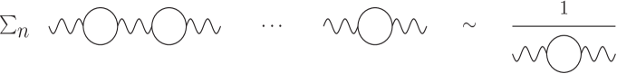
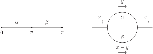
The basic approach in these low dimensional theories was to exploit the fact that the real parameter of the (flavour) symmetry group could order the Feynman graphs contributing to a Green’s function differently to the ordering defined by the loop expansion of coupling constant perturbation theory. For instance in the large method [69] the generic coupling constant was given a notional dependence by requiring that the combination was held fixed in the large limit which is . Therefore the leading order or dominant graphs contributing to a Green’s function corresponded to those where there were chains of bubbles of matter fields which are illustrated in Fig. 1. Consequently one bubble gave a factor of to the value of the graph which with the associated two coupling constants meant that a chain of bubbles had the same notional dependence as any other chain.

To illustrate this we recall the basic formulation of both the nonlinear sigma model [68] and Gross-Neveu model [69]. The former has the Lagrangian
| (2.1) |
where , is the coupling constant and is a Lagrange multiplier field which ensures that the scalar fields lie on the sphere . This is the coordinate free version of the model. Eliminating the constraint will introduce a set of coordinates for each coordinate patch but for the large approach (2.1) is used. In the case of the Gross-Neveu model we have [69]
| (2.2) |
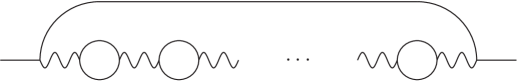
where is a fermion, is the coupling constant but now in this case is an auxiliary field. This can be eliminated from (2.2) to produce a theory with a quartic fermion self-interaction. That formulation of (2.2) is more appropriate to use if one is carrying out explicit perturbative computations in two dimensions which is the theory’s critical dimension. As there is only one vertex in both (2.1) and (2.2) then at leading order in the large expansion one diagram contributing to the field -point function is given in Fig. 1 where the dots indicate the addition of other bubbles of or fields. Irrespective of whether the fields are massive or not all graphs in the sequence are of the same order in large . To summarize, summing up the graphs produces a geometric series which is formally illustrated in Fig. 2. Our representation of the process in this figure is schematic because for different theories the actual outcome of the summation depends on the structure of the underlying Lagrangian. For instance in (2.2) the quadratic term in is part of the summation but there is no corresponding term in (2.1). In either the massive or massless case the explicit value of the bubble can be determined for the theory of interest and the large form of the propagator can be found. We will give an example of this shortly. Also as we will be discussing theories which are similar in structure to (2.1) and (2.2) later from this point of view we note that the respective interactions are what we term as core and in fact each define a separate universality class. Within each a sizeable number of field theories are equivalent. In this context we will refer to the field and its later equivalents as the force field. The fields to which it couples through this common interaction and which lie in the flavour group will be termed the matter fields. For our examples these are clearly and of the two respective Lagrangians.
2.2 Dynamical mass generation
One of the early interests in studying quantum field theories via the large expansion rested in the fact that nonperturbative properties can be studied. At this point it is worth noting that our use of the word nonperturbative here means the zero instanton sector where the small coupling constant expansion is around the free field solution. In other words we are not in a sector where there is a perturbative expansion around a classical extended object or solution such as a breather, kink, monopole or dyon. These latter quantities sometimes are included in the overall banner of nonperturbative in the nonanalytic sense. So for us nonperturbative now means the summation of perturbation theory in the zero instanton and zero extended object sector. Given this it transpires that both (2.1) and (2.2) possess rich nonperturbative properties. In the perturbative expansion of the theories around zero coupling constant if the matter fields and are originally massless then they remain so. However the perturbative vacuum in each case is not stable and there is a more energetically favourable vacuum solution which is not perturbatively accessible. In that vacuum there is dynamical mass generation whereby the matter field of each Lagrangian becomes massive. Moreover the apparently nonpropagating field of both theories develops a nonfundamental propagator. In effect each becomes a bound state of two matter fields as is suggested by the graph of Fig. 2. In the perturbative formulation of both (2.1) and (2.2) the field is not present. In the case of (2.1) eliminating the Lagrange multiplier constraint by choosing a coordinate system for the underlying manifold gives
| (2.3) |
where and is the metric of the coordinate system chosen for the patch which includes the free field case. The coupling constant appears implicitly in the metric. In the case of the Gross-Neveu model there is a parallel re-expression. Eliminating the field of (2.2), as noted earlier, produces the purely fermionic Lagrangian [69]
| (2.4) |
In both cases there is clearly no mass term for each matter field and, moreover, none is generated or apparent in any perturbative expansion.

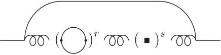
To access the dynamical mass generation one has to construct the effective potential for the field in both cases. For instance, using (2.2) one sums up the leading order graphs with field insertions on a closed fermion loop which are illustrated in Fig. 3. This produces the effective potential which is
| (2.5) |
at leading order for (2.2) where is the point where the divergences are subtracted [69]. The first term is clearly the canonical quadratic one of the original Lagrangian which would lead to the solution classically for the vacuum expectation value of . With quantum corrections included this classical vacuum is not the only turning point of as there is a second one at
| (2.6) |
which is a global minimum. The one with corresponds to a local maximum meaning that the perturbative vacuum is unstable. With the nonzero vacuum expectation value for the fermion develops a mass dynamically. From (2.6) one finds that this mass depends on the coupling constant nonanalytically. Such a dependence on means that the dynamical mass has a zero asymptotic expansion near and hence not accessible perturbatively. What has transpired is that the true vacuum of the theory has been accessed or touched in the large summation of graphs in our nonperturbative meaning. Though it is worth stressing that while it has been accessed it has been done so within an approximation at leading order only. Exploring the scenario to higher precision requires corrections which are technically very difficult to carry out when the nonzero dynamically generated mass is present. Several studies in this direction can be found in Refs. [70, 71] and [72].
However, the existence of the mass gap in this theory given by (2.6), revealed via the leading order large approach, has been refined by the determination of the mass gap of (2.1) and (2.2) exactly [73, 74, 75, 76] from the explicit form of the exact -matrix which was constructed in Refs. [77, 78, 79] and [80]. The large expansion has been used to check the exact expression [81, 82]. In the former case the corrections to the fermion -point function in the Gross-Neveu model were computed using (2.8) in dimensional regularization where tadpole graphs have to be included. The latter large check was carried out by computing the -point function for the nonlinear sigma model at but with lattice perturbation theory. Indeed it is possible to use this large lattice regularization approach to extend analyses to for the nonlinear sigma model [83]. Equally another check on the exact -matrices proposed for (2.1) and (2.2) centred on the assumptions behind the construction. In two Minkowskian spacetime dimensions particles can only move along a line which puts a restriction on scattering. For theories with an exact -matrix it was assumed that there is no scattering and for three particle scattering the order of the constituent scatterings was immaterial [77, 78, 79, 80]. In the former case this has been checked explicitly in several cases in the large expansion [77, 78, 79, 80, 84] using the Källén-Toll cutting rule [85]. This rule is specific to massive two dimensional Feynman integrals and allows one to express finite one loop integrals as a sum of tree graphs. The premise behind its usefulness is the same as that for the exact -matrix construction in that particles can move in only one of two directions in two dimensions. This allows one to express momenta in a basis determined by the light cone and exploit properties of complex analysis [85]. Applying the rule in the case of the scattering the leading order large one loop graph is cut open in such a way that its contribution is equal and opposite to the sum of all six tree graphs which ensures that there is no production in these theories. By contrast another useful cutting rule was provided in Ref. [86] for evaluating a class of massive integrals occurring in large computations. The underlying mathematics is one of the Gauss relations of the hypergeometric function.
Equipped with this knowledge we can return to (2.2) and reconsider it. While the conventional way of calculating perturbatively in the Gross-Neveu model is to use the Lagrangian (2.4) perturbation theory can also be carried out in (2.2). For instance, this has been achieved in Ref. [87] at three loops. We mention this work as it is relevant to the large approach. While we have noted that the true vacuum has one can still perform perturbative computations in (2.2) with . This is achieved by noting that the so-called propagator of in the classically unstable vacuum is unity. In other words it is momentum independent. The technical exercise in doing such calculations can be viewed in Ref. [87]. However, (2.2) is not perturbatively renormalizable multiplicatively [87, 88, 89] since the fermion -point function is not finite. Therefore an extra interaction needs to be appended to the Lagrangian (2.2) for perturbative computations which is that of (2.4) but with a different coupling constant. Despite this the three loop -function of the Gross-Neveu model was computed for the coupling constant which was in agreement with the independent computation of the -function carried out at the same time in Ref. [90]. While the original and main motivation of Ref. [87] was to construct in perturbation theory to three loops for the present consideration it illustrates that it is technically possible to use (2.2) for computations in the classical vacuum. Earlier loop calculations of the renormalization group functions in (2.2) were carried out over several years in Refs. [91, 92] [93]. In noting that (2.2) is not formulated in a way that is perturbatively renormalizable, we need to clarify that neither (2.2) nor (2.4) are multiplicatively renormalizable when dimensionally regularized [88, 89, 94, 95, 96]. This is because in using this regularization evanescent -point operators are generated which spoil the multiplicative renormalizability and is only a feature of two dimensional theories with -fermi interactions. In the case of (2.4) the first order where such an operator appears is three loops [96, 97] and its effect in the renormalization group functions will not be manifest until four loops [98, 99]. However, the formalism developed in Refs. [88] and [89] to handle these evanescent operators in two dimensional -fermi theories, where they first arise at a lower loop order than (2.2), can be applied to the Gross-Neveu case to allow one to extract the correct four loop renormalization group functions [98, 99]. For instance, as the theory is free the -function has to be proportional to . Without knowing about the generation of the evanescent operators or using a formalism to accommodate their effect, this factor would not appear in the -function at four loops [99].
Given that the effective potential of (2.2) determines the true vacuum to be we can introduce the new field by
| (2.7) |
where . Then (2.2) becomes
| (2.8) |
where we have omitted the constant term. The linear term in is retained as there are tadpole corrections to the -point and other functions which play a crucial role in ensuring the quantum theory is consistent for a nonzero . Further technical details on this can be found in Refs. [86] and [100]. As this is the form of the Lagrangian in the neighbourhood of the true vacuum we can examine it in the large formalism. With the field develops a propagator which can be deduced from the sum of graphs in Fig. 2. In particular at leading order in the propagator is
| (2.9) |
where
| (2.10) |
in two dimensions. This is clearly a nonfundamental propagator with a pole at from the prefactor. It corresponds to the bound state of two fermions. Higher order large corrections will adjust the bound state mass from this leading order value. This can be seen from an alternative point of view. The full mass spectrum of the theory can be adduced from the exact -matrix of the Gross-Neveu model which is given in Refs. [77, 78, 79] and [80]. For example it provides the full spectrum of particle excitations and their masses including that of dynamically generated field. As an aside the exact -matrix and the bound state particle masses are a function of for the theory rather than alone. Indeed it should be the case that if one could compute higher order corrections the large expansion the quantity of interest these additional terms should be such as to produce a expansion. The presence of this factor is the dual Coexeter number of the group and is not unrelated to the fact that (2.4) corresponds to a free field theory at as already noted.
One aspect of (2.9) which will be important for later is the form of the propagator in -dimensions. This can be determined from the dimensionally regularized evaluation of the one loop bubble graph on the right hand side of the equation in Fig. 2. In particular
| (2.11) |
where is the hypergeometric function. So in the massless limit
| (2.12) |
While this corresponds to a canonical propagator in four dimensions the -fermi interaction is nonrenormalizable in perturbation theory in that spacetime. However it transpires that this propagating field will play a role in the critical point dynamics of the Gross-Neveu model at the Wilson-Fisher fixed point in -dimensions which will be discussed later.
2.3 Lagrangian reformulation
As it stands (2.8) contains a massive fermion with a propagator which can be deduced by conventional means. While the large expansion has revealed that the field is dynamical with a propagator albeit nonfundamental the latter is not present at the outset. In Refs. [34, 100] and [101] the effective Lagrangian description of this scenario in the true vacuum has been addressed. Conventional quantum field theory at the defining stage writes the action as a free part and an interacting piece with . How the split is made is entirely an open choice as there is not a unique way of defining . For instance in (2.8) the mass term could be included in the Lagrangian of or . If it is present in the former one develops the field theory with a massive fermion. By contrast if it is present in one has a massless fermion but also a -point vertex independent of the coupling constant. In this situation at each loop order one has to include an infinite number of insertions of this -point vertex in all the graphs. The consequence of this is to reproduce the massive fermion propagator through a geometric series similar to that of the large bubble sum. In other words while the split in the Lagrangian is not unique the results obtained are ultimately independent of how it is carried out. An analogous process underlies the observation of Refs. [34, 100] and [101]. To accommodate the fact that the field has a nontrivial propagator in (2.8) at the outset it is included redundantly in a bilocal way
| (2.13) |
where is the coordinate space representation of the one loop bubble of Fig. 2. When this is a complicated function which is related to (2.11) but simplifies substantially when . This formulation (2.13) allows one to carry out the formal large development and renormalization [34, 100, 101] from a Lagrangian standpoint as it corresponds to the (effective) field theory active at the true (nonclassical) stable vacuum. While both the Gross-Neveu and nonlinear sigma models are two dimensional asymptotically free field theories with matter fields, which are massless in the classical vacuum, the dynamical generation of mass in the true vacuum is one of the reasons they have been studied. This is because several of these properties are shared by QCD in four dimensions.
While the field plays a role similar to the QCD gauge field which is massless, low energy lattice gauge theory evidence has accumulated over the last decade that indicates that the gluon appears to have an associated nonzero mass scale. This derives from studies of the gluon propagator in the Landau gauge initiated in Ref. [102]. At zero momentum it appears that the Landau gauge gluon propagator freezes to a nonzero value. This is not indicative of a mass for the gluon in the fundamental sense as the gluon propagator does not have a simple or higher order pole at any nonzero momentum. A simple pole would imply the gluon was visible and contradict the expectation that it is a confined quantum. However it does suggest the presence of a mass gap for the gluon which has a parallel in the nonlinear sigma and Gross-Neveu models. By contrast neither have confinement of the matter or force fields. However as colour confinement in QCD is a low energy phenomenon one assumption is that it could have a Lagrangian prescription which is not local. This was one property uncovered by Gribov in his seminal work [103] on the consequences of not being able to globally fix a gauge uniquely in a nonabelian gauge theory. Another avenue to pursue might be to adapt structures such as (2.13) to the Yang-Mills or QCD situation. An example of a related approach was provided in Refs. [104] and [105] to tackle the confinement of quarks. There in a model where the spin- fields were regarded as massive the gluon fields were integrated out of the action to produce an effective low energy theory involving only quark fields. These were subsequently eliminated in favour of bilocal fermionic objects. An underlying assumption in that construction was the nonzero mass for the gauge field in the Lagrangian. While pre-empting the proof of a mass gap for the gluon such effective low energy theories could not be countenanced without the presence of some sort of mass scale, whatever its origin, which clearly is in contradiction with the gauge action principle. A not unreasonable way to view this would be that such masses emerge dynamically or can be accommodated in an effective theory situation akin to those seen in the large expansions of the simple two dimensional theories of (2.1) and (2.2).
2.4 Spin- theories
To complete this chain of reasoning in the present context one way of accessing mass gaps is via large expansions. For a spin- nonabelian field the analogous theory to develop a large expansion for is the two dimensional nonabelian Thirring model (NATM) with Lagrangian [106, 107]
| (2.14) |
where are the generators of the Lie group of the colour symmetry. In this model and the QCD case the range of the flavour index will be regarded as where is the number of quarks. This is to distinguish it from the number of colours of the gauge group as where is the dimension of the adjoint representation of the Lie group. To effect a Lagrangian formulation which is analogous to those of (2.1) and (2.2) a spin- auxiliary field in the adjoint representation of the Lie group is introduced to give
| (2.15) |
If one were to continue the parallel with (2.1) and (2.2) in two dimensions then the field would become dynamical in the true vacuum of the theory. This would be apparent via the effective potential of the composite field analogous to which is in (2.15). At this stage this reasoning breaks down as a nonzero vacuum expectation value for the auxiliary field is not possible as the colour symmetry would be broken. Moreover this is for a simple two dimensional model of the process rather than the four dimensional gauge theory. However we will discuss the usefulness of (2.15) in the large context for extracting information on the renormalization group functions in QCD later motivated by observations provided in Ref. [108]. In addition that article explored the consequences of the proposal that the gluon could be regarded as the bound state of two quarks. This is not nonsensical since a confined object may not be a fundamental entity.
Despite the apparent possibility of extending the dynamical mass generation properties of (2.1) and (2.2), exposed via the large expansion, to models with nonabelian composite fields an alternative tack has been developed in a series of articles [109, 110, 111, 112]. A formalism, now termed the local composite operator (LCO) technique, was applied to Yang-Mills and QCD in Refs. [112] and [113] respectively. In the LCO approach an effective potential can be constructed for the composite field in the case of (2.2) in Refs. [109] and [110] and in the gauge theory case in the Landau gauge. An early attempt to construct a perturbative potential for the composite operator in the Gross-Neveu model was given in Ref. [87]. Although that was a three loop computation using (2.2) the resulting effective potential did not satisfy a homogeneous renormalization group equation. By contrast the LCO construction embeds homogeneity within the development of the effective potential. Moreover the effective potential can be derived using standard perturbative techniques. In the gauge theory case the expectation value of the gauge field composite is nonzero and leads to a new more energetically favourable vacuum where the gluon becomes massive. Interestingly the anomalous dimension of the composite operator in the nonabelian gauge theory is not independent in the Landau gauge and satisfies a simple Slavnov-Taylor identity being the sum of the gluon and ghost anomalous dimensions. This was first shown in Ref. [114] and independently observed in a three loop renormalization in Ref. [115]. A more in depth all orders proof was subsequently provided [116]. Amusingly the mass parameter associated with the nonlocal dimension zero operator introduced in Gribov’s model of colour confinement has the same renormalization property as the dimension two gluon mass operator in the Landau gauge [117, 118].
3 Large renormalization group functions via summation
While we have concentrated on the application of the large expansion to reveal properties of the true vacuum of (2.1) and (2.2) the technique can also be used to extract information on the renormalization group functions. Early work in this respect was pioneered in Refs. [64] and [65] for the case of QED. Later applications have been to supersymmetric theories [119, 120], before enjoying a renaissance for gauge-Yukawa theories in order to explore ideas about physics beyond the Standard Model [121, 122, 123, 124, 125]. One idea is to understand the effect a large number of fermions with a vector rather than Yukawa interaction has in a gauge theory and whether asymptotically safe scenarios can be accommodated [121, 122, 123, 124, 125].
3.1 QED
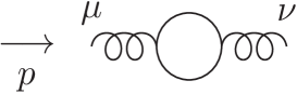
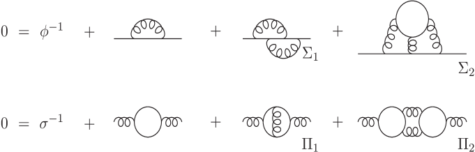
The basic idea of Refs. [64] and [65] is to determine the contribution to the renormalization constants by first evaluating diagrams where chains of massless bubbles in the large approximation are included in the Green’s function such as that shown in Fig. 4 before carrying out the full renormalization at leading order. In other words where a force field propagator such as ordinarily appears in a Feynman diagram the propagator is replaced by one with a series of matter field bubbles. The final renormalization procedure followed is exactly the same as in perturbation theory where coupling constant and wave function counterterms are included where appropriate in the chains of graphs. The determination of the leading order part of the renormalization group functions is then carried out in the scheme.
One of the main features of the original approach of Refs. [64] and [65] for QED is that these graphs with bubble chains can be resummed and the overall Feynman diagram evaluated leading to a one parameter integral representation of the leading order large renormalization group functions. Here will be the number of electron flavours which we will denote by . Even though there is no colour symmetry, leading order QCD data can be deduced in some instances [65]. The resummation in effect corresponds to the replacement of the canonical power of the photon in the chain of Fig. 4 with the full critical exponent including the anomalous dimension making it ultimately equivalent to the starting point of the critical point large formalism of Refs. [34] and [35] which will be detailed later. However, the resummation method has been revisited recently in the context of extending gauge theories to include the effect of Gross-Neveu-Yukawa type interactions and extensions where the motivation to is to explore the possibility of new fixed points in generalizations of the Standard Model. The general area fits within exploring the existence and consequence of the asymptotic safety ideas introduced by Weinberg [126]. For instance, see Refs. [121, 122, 123, 124] and [125] for recent work applying the summation method of Refs. [64] and [65] to directly find the large renormalization group functions for such gauge-Yukawa extensions of the Standard Model.
It is best to briefly outline aspects of the procedure of Refs. [64] and [65] with an explicit example where the large contribution to a renormalization group function is determined directly by the summation method. We consider the contribution to the Landau gauge electron wave function renormalization from the sequence of graphs given in Fig. 4. In practical terms the building block graphs are illustrated in Figs. 5 and 6 and are simple to evaluate in QED. For instance the graph of Fig. 6 gives
| (3.16) |
in general or
| (3.17) |
when . This is included as the amputated photon -point bubble in Fig. 5 prior to completing the integral. The evaluation of the graph of Fig. 5 comprises several parts. The momentum independent part of (3.17) is factored out of the final integration as are the associated counterterms. One aspect of the graph of Fig. 4 worth noting is that we have grouped the bubbles together separate from the counterterms. In practice it represents all possible different distributions of the bubbles and counterterms from the binomial expansion of their sum. As the momentum through each contribution is the same within the final Feynman integral then the representation of Fig. 5 corresponds to all contributions to the loop order. What remains to complete is the final integration which is of the form
| (3.18) |
Consequently there is a complicated contribution to the electron -point function at loops given by [64, 65]
| (3.19) |
where
| (3.20) |
with . While this corresponds to the final contribution of the sequence of graphs to the leading order electron -point functions the extraction of the part that leads to the renormalization group function follows the same procedure as in perturbation theory. When the counterterms are appended one only needs to isolate the simple pole in . At leading order in large this is possible and the residues of this simple pole can be written as a sequence. While the method to achieve this is involved the solution leads to a one parameter integral representation of the electron anomalous dimension. One benefit of this method is its range of applicability to several related theories of current interest [121, 122, 123, 124, 125]. However to go to the next order in by this approach would require a significant amount of tedious resummation of graphs with not only more than one bubble chain but also corrections to the basic bubble of Fig. 6. While this sketch focused on the electron wave function renormalization it has been extended in QED to the -function [65] using the same underlying procedure and a one parameter integral representation found for the piece. An example of this will be given in (6.79). The alternative critical point formalism will reproduce this which we will comment on later.
3.2 Renormalon connection
One related aspect of this summation approach to large expansions concerns the presence of renormalons and accessing their effect within a Green’s function. It is widely accepted that the perturbative expansion has limitations in its range of applicability. The obvious case is that the expansion parameter, which is invariably the coupling constant, is small. Ultimately one would want to extend the range of convergence of a perturbative series and in an ideal scenario this would mean computing all possible contibutions to a Green’s function which is clearly unrealistic for the main theories describing Nature. An alternative would be to probe beyond the lowest orders by summing up classes of graphs contributing to a Green’s function rather than to gain insight into the coefficients of a renormalization group function as the main motivation. In effecting such summations as a function of the coupling constant the resultant function can have poles for positive values of the coupling constant. Such poles are an obstruction to the summation and extracting a value for the Green’s function for a value of the coupling constant beyond the pole closest to the origin will not give reliable values. Such a pole is usually regarded as a renormalon and indicates that there may be a missing contribution to the series [127, 128]. In other words it indicates the location of a nonperturbative contribution which cannot be accessed directly via conventional perturbation theory. More recent thinking [121, 122, 123, 124, 125] has suggested that it might be an indication of a new type of fixed point applicable to ideas of asymptotic safety and models for new physics beyond the Standard Model.
In practical terms the simplest summation of graphs which can be used to study such renormalon poles is the elementary bubble chains of the large expansion such as the graphs in Figs. 4 and 5. While the contributions to the bubble chains in a Green’s function can be deduced by following the resummation process discussed earlier an alternative way is to observe that the large bubbles which are relevant occur in the photon or gluon in the case of QCD propagator. Moreover each bubble gives the same contribution. Therefore the summation can be efficiently implemented by using
| (3.21) |
rather than the usual propagators where would be zero. Here where is the coupling constant and is the Dynkin index of fundamental representation of the QCD colour group. In other words represents the contribution from each individual bubble in the gauge field chain of Fig. 4. As an application of this method we note that the photon propagator in QED has been considered in Refs. [129, 130] and [131], for example. Another instance arises in deep inelastic scattering where QCD is used to compute the Wilson coefficients [132, 133]. For example is the flavour nonsinglet longitudinal structure function and its coefficients have been determined at leading order in and expressed compactly in [131]
| (3.22) |
Here corresponds to the number of loops, is the Bjorken scaling variable, is the rank colour group Casimir and . If one effects the th order derivative then the coefficients are in exact agreement with the known three loop perturbative coefficients [134]. Therefore one can regard (3.22) as representing the resummed set of graphs. What is evident from the expression is that there are poles when is or and these correspond to renormalons with the first obstruction at unity.
While one can estimate the location of the renormalon from the pole one has to be aware that in QCD the large expansion is in effect in the QED sector of the gauge theory. For the colour group when then QCD is no longer asymptotically free. Therefore to circumvent this difficulty the process of naive nonabelianization was introduced in Ref. [135] and discussed in Refs. [136] and [137], for instance. Instead of referring to a large expansion one uses a large expansion. Here is the one loop coefficient of the QCD -function and given by
| (3.23) |
where is the rank two colour group Casimir in the adjoint representation. So when a Green’s function has been determined in large the naive nonabelianization is implemented by the replacement
| (3.24) |
and is used as the expansion parameter for the Green’s function. The effect of this has been studied in Ref. [135] and an improvement in comparison with known two loop estimates has been noted for different quantities. As an aside this replacement is not unreminiscent of the use of rather than in the large expansion in the Gross-Neveu and nonlinear sigma model in two dimensions noted earlier. In that case, however, the -matrix is known exactly and the dependence on is evident. In higher dimensions there is no guarantee that the -matrix of QCD should be a function of per se. One final comment on this aspect of large expansions to the properties of Green’s functions in general is that the examples we have indicated for finding renormalons has been limited to single chain cases. While there has been studies of cases where there are two gauge propagators corresponding to double chain expansions, the full analysis of such Green’s functions is technically very difficult. This is because one has to evaluate the underlying core finite Feynman diagrams where two of the propagators have a power involving . Moreover since corresponds to a certain number of inserted bubbles when there are two such propagators one has to have two different exponents. This further complicates the evaluation of the basic graphs. However progress in this direction in large QED has been provided in Ref. [131].
4 Large critical point formalism
The large formalism of Refs. [34] and [35] follows the same principles of perturbative quantum field theory in the sense that one has to evaluate the core Feynman diagrams contributing to Green’s functions. What the essential difference though is that in perturbative quantum field theory the propagator of a scalar field, for example, has unit power. This is because one is perturbing around the Gaussian fixed point of the theory or equivalently in the neighbourhood of a free field and one determines the canonical dimensions of the fields by ensuring the action is dimensionless in the critical dimension. By contrast in the critical point large formalism [34, 35] one is close to the critical region of the Wilson-Fisher fixed point [37, 38, 39, 40] in -dimensions. At this point the critical theory, being away from the critical dimension of the theory, is not free but interacting. These two starting points differ as we have discussed earlier in our examples of (2.1) and (2.2). One starting point relates to the theory in the conventional perturbative expansion whereas the other corresponds to the theory in the true stable vacuum.
4.1 scalar theory
For illustration we focus on the simple case of the nonlinear model in the formulation of (2.1). It has critical dimension and in perturbation theory the free theory involves only the scalar kinetic term which produces the canonical (massless) propagator where is the momentum of the field. This form of the scalar propagator is universal across all spacetime dimensions. Equipped with this one computes, for instance, the renormalization constants of the fields and parameters, such as the mass and coupling constant, which are the essential quantities for evaluating any Green’s function. The consequent renormalization group functions can be derived and these in effect are a measure of the radiative or quantum corrections of the underlying theory. For instance, the anomalous dimension of , denoted by , quantifies the shift of the dimension of the field from its canonical or classical dimension. In other words the fields and the operators built from those fields do not have the classical dimensions when in the interacting quantum theory.
By contrast the large critical point approach begins from a nonfree Wilson-Fisher fixed point, , defined by the nontrivial zero of the -function
| (4.25) |
and hence the corresponding canonical dimensions of the fields across dimensions are noninteger. To deduce their canonical values one performs a simple dimensional analysis of the Lagrangian in dimensions with the premise that the action remains dimensionless for all . Therefore from (2.1) the dimension of is since the measure in the definition of the action introduces the dimension dependence where we will use the shorthand that
| (4.26) |
throughout. In addition the interaction of (2.1) is noninactive in this analysis since we are at the Wilson-Fisher fixed point. It therefore defines the canonical dimension of as in all dimensions since the coupling constant has been scaled into what we call the spectator term. Therefore the matter field and the core interaction determine the scaling dimensions of the fields in the universal theory from which one defines the propagators used to evaluate Green’s functions in the large formalism [34, 35]. In addition one can exploit the fact that at criticality the fields are massless. Therefore the radiative corrections to a propagator as it is iterated order by order within the Green’s function can be resummed. The consequence of this is that those radiative corrections exponentiate at criticality to add an additional term in the exponent of the propagator. It is quantified explicitly as the renormalization group anomalous dimension of the corresponding field but evaluated at the value of the critical coupling constant. In practice this is ordinarily a small number. Within the large construction, however, the corresponding anomalous dimension exponent will be a function of [34, 35]. Only when evaluated at an integer dimension can it be compared to computations by other techniques. The upshot is that the propagators of the critical nonlinear model are not the usual ones associated with perturbation theory but take the leading order form
| (4.27) |
in the asymptotic scaling region of the Wilson-Fisher fixed point. It is these forms which are used in the large critical point formalism [34, 35]. They have been formulated in coordinate or -space as the dimensional analysis was for the -space version of the Lagrangian. If the momentum space of (2.1) had been used then the propagators would have been
| (4.28) |
These sets of propagators are connected via the Fourier transform which in the conventions of Refs. [34] and [35] is
| (4.29) |
where we define
| (4.30) |
as the shorthand for the combination of Euler -functions which appear [34, 35] and . In both sets of propagators an arbitrary -independent amplitude is present such as which can be determined within the large expansion with the momentum space amplitudes related via the Fourier transform. We use the convention that matter field amplitudes will be denoted by and the corresponding force field will be denoted by where is a generic field. Finally, the exponents are defined by
| (4.31) |
In the latter relation the exponent represents the anomalous dimension of the vertex operator***In the original work of Refs. [34] and [35] the letter was used for the vertex operator anomalous dimension. . In general each operator has an anomalous dimension which corresponds to an independent renormalization constant in perturbation theory. Therefore one has to allow for the analogous exponent in the critical point large formalism.
Having defined the asymptotic scaling form of the scalar propagators in both coordinate and momentum space one can readily deduce analogous expressions for the related -point functions. These are necessary as one method to deduce the wave function critical exponent for the matter field is to solve the skeleton Schwinger-Dyson equations for the -point functions of the theory [34, 35]. In momentum space these are given by merely inverting the scaling forms of (4.28) to give
| (4.32) |
The coordinate space counterparts are deduced by applying the inverse Fourier transform to give
| (4.33) |
where
| (4.34) |
and we have mapped one coordinate to the origin without loss of generality.
While we have introduced the leading order structure of the propagators in the asymptotic limit to the fixed point in (4.27) corrections to these can be included. They have the form
| (4.35) |
where and are the associated coordinate independent amplitudes. The scaling forms of the -point functions are derived in the same way as before producing [34, 35]
| (4.36) |
where
| (4.37) |
The exponent is a generic one for the correction term. For instance, it could be regarded as the exponent corresponding to the critical slope of the -function. The evaluation of the -function at the fixed point clearly cannot correspond to a nontrivial exponent due to (4.25). However, it could correspond to another exponent such as that relating to the specific heat for instance. For scalar theories, for instance, the correction term is in effect equivalent to zero momentum insertions on a propagator line and therefore such terms identify -point functions. The new amplitudes tag the parts of the Feynman graphs which contribute to this. In perturbative field theory computations a similar technique is used to extract renormalization constants for mass operators where the zero momentum insertion does not give rise to infrared divergences. An example of such an application is the three loop renormalization of the quark mass operator in the scheme in Ref. [138]. So the correction terms of (4.35) should be regarded as insertions of -leg operators with possibly derivatives included.
For instance the -function of the nonlinear model and theory have both been determined at in Refs. [34, 35] and [139] by this method using the universal theory with the same core interaction which is that given in (2.1). In the former theory the canonical term of the correction exponent was . For the latter it was as the coupling constant of four dimensional theory is dimensionless when . To understand the commonality of both theories it is best to recall the theory Lagrangian which is the four dimensional partner of the two dimensional nonlinear sigma model, (2.1). Taking the usual four dimensional Lagrangian which is
| (4.38) |
then analogous to (2.4) this can be rewritten as
| (4.39) |
which clearly shares the same interaction as (2.1). With both (2.1) and (4.39) the noncommon dependent pieces define the canonical dimensions of the respective coupling constants. In the former case the dimension is but in the latter. It is these exponents which are separately used in the correction to scaling parts of the asymptotic scaling functions of (4.35) when they are inserted in the skeleton Schwinger-Dyson equations which will be discussed in detail later. The connection of these canonical parts of the exponents with the respective -functions is that they correspond to the critical slopes of the -functions. In a dimensionally regularized perturbative computation the coupling constant has a nonzero dimension in -dimensions. This is reflected in the -dependence of the leading order term of the -function. In mentioning how the exponents of the -functions are computed in relation to the structure of the universal Lagrangian we note that these are examples of hyperscaling laws. Another example in (2.1) can be deduced for the dimension of the mass dimension. The mass operator is which also couples to the field. Therefore the mass anomalous dimension for corresponds to the anomalous dimension of the field. By contrast the mass of the field is deduced from its mass operator which is . In other words when the critical dimension is six the anomalous dimension of the mass of , which will then be a propagating field, is related to the -function of theory.
4.2 Early connections
In discussing the critical point large formalism to this we can now connect it with other approaches using expansions. The method of Refs. [64] and [65] which explicitly summed the chains of bubbles in the massless theory to extract the renormalization group functions at leading order overlaps with the construction of Refs. [34] and [35]. For instance in Refs. [64] and [65] the bubble sum produced a propagator with a -dependent exponent. Equally in the massive case discussed in the context of the Gross-Neveu model the auxiliary field becomes dynamical and the -dimensional propagator has a -dependent scaling form when the generated mass is set to zero as indicated in (2.12). Both these consequences are accommodated naturally in the asymptotic scaling forms of (4.27). For instance the propagators (2.12) and (4.28) are equivalent at leading order. Likewise the overall summed propagator of Fig. 4 leads to an exponent equivalent to that of the field of (4.27). Moreover the technique of Refs. [64] and [65] produces the leading order large renormalization constants and consequent renormalization group functions. These connections are related since they are the same quantity but derived in different ways. The advantage of (4.27) is that the scaling forms transcend the critical dimensions of the specific theories and are the propagators in the universal critical theory bridging all theories in the same universality class. Moreover while the leading order behaviour of the exponent is deduced on dimensional grounds the anomalous terms such as and in (4.31), for instance, correspond to quantum corrections. In effect they quantify the contributions from graphs of the form of Fig. 4. Given this when one uses (4.27) in critical point large calculations there is no dressing of the propagators with bubble chains. These contributions are already summed in the exponent. Consequently one has to compute massless Feynman graphs with nonunit powers unlike conventional perturbation theory. Massless field theory techniques have been developed for this and we discuss some of these in Appendix A with several examples in Appendix B.
At this stage it is worthwhile introducing some basic graphical notation concerning the evaluation of Feynman graphs for massless theories with nonunit propagator powers. We do this in the context of the simple Feynman integrals given in Fig. 7 where and are arbitrary complex parameters here and each graph corresponds to the same integral which is [34, 35]
| (4.40) |
where
| (4.41) |
This integral corresponds to both graphs of Fig. 7 since they are different graphical representations. In the left hand graph the vectors comprising the two propagators are placed between points on the plane with reference to some origin. The two endpoints and are regarded as fixed and the variable to be integrated over can be anywhere else on the plane although we have chosen to place it at the centre of the connecting line. The more conventional way of graphically representing the integral is given in the right hand graph of Fig. 7 where is the loop momentum and the external momentum. It is worth recognising the flexibility which both representations present. For instance, an integral in momentum space can be represented in a coordinate space way where the and are replaced by the more conventionally used letters. Irrespective of which is adapted both will reflect underlying symmetry properties much more clearly than the explicit integral itself especially in higher loop graphs. Equally some integration rules, which we discuss later, are easier to apply in one representation over another.
4.3 Skeleton Schwinger-Dyson equation
Equipped with these tools we can now illustrate the core strength of the large formalism of Refs. [34] and [35]. For this we use (2.1) as the basic theory and note that the -point functions of the fields are shown in Fig. 8 to . In the large counting a field is regarded as one power of and each closed loop contributes one power of . Therefore the final two graphs of each equation in Fig. 8 are the same order in . By contrast they would be different orders in the coupling constant expansion. We have chosen to use (2.1) rather than (2.2) as in the latter case the final two graphs of each equation in Fig. 8 would be zero due to the trace over an odd number of -matrices and this large graph ordering would be less apparent. In either case we have not included any dressings on the propagators since the presence of the anomalous dimensions in the critical propagators (4.27) and (4.28) already represent those summations. Using the coordinate space propagators the equations of Fig. 8 are formally represented by
| (4.42) | |||||
to the first two orders in large where we have defined the combination of amplitudes to be and the external coordinates of all graphs are and . The quantities and are the -independent values of the respective graphs of Fig. 8. In practice their values are divergent not unlike their perturbative counterparts and their determination requires a regularization. As the formalism [34, 35] operates in the universal field theory in -dimensions, where is arbitrary, dimensional regularization cannot be used for this task. Instead graphs are regularized by the dimensionless quantity , which is regarded as small, and is introduced by shifting the vertex anomalous dimension via
| (4.43) |
which is the origin of the extra term in each of the powers of the coordinate in (4.42).
In dimensionally regularizing a field theory for perturbative calculations the regularizing parameter is introduced by modifying the spacetime dimension which changes the dimensionality of the coupling constant. This is the parameter of the perturbative approximation. Here the situation is similar in that one is in effect performing a perturbative expansion in the vertex anomalous dimension which is why that parameter is formally modified. Thus we can define the general divergence structure of each graph by
| (4.44) |
There will be terms but these are not relevant for an computation. The equality of the poles is not an error but a reflection of the result of the explicit evaluation. More deeply it demonstrates the underlying large renormalizability of the theory which has been discussed in depth in the critical point context in Refs. [140, 141] and [142]. Similar renormalizability arguments apply equally to (2.2) and other theories which are accessible via the large critical point formalism. Indeed these are not unrelated to the early discussion of the large renormalizability of the Gross-Neveu model in dimensions greater than observed in Refs. [63] and [143]. As the equations of Fig. 8 have divergences these are removed by the counterterms available from the vertex renormalization constant present in (4.42). We have only included it in the leading order terms since it plays no role at . It would only be required there if one was extending the equations to the next order in . The structure of is formally similar to that of renormalization constants in conventional perturbative calculations and takes the form [141]
| (4.45) |
where are the counterterms and depend on . They can then be expanded in large via [141]
| (4.46) |
Aside from the fact that the Schwinger-Dyson equations are divergent and require renormalization there is an additional aspect to their structure. As the ultimate aim is to study them in the critical region in the approach to the fixed point where there is scaling, we will have to take the limit. While it looks as if this is not a problem from the structure of (4.42) the divergent graphs mean that there are terms when the exponent is expanded for small . For (2.1) these are excluded by defining the vertex anomalous dimension by [34, 35]
| (4.47) |
We use the notation that exponents and amplitudes such as have the expansions
| (4.48) |
Since (4.47) involves the simple poles of the graphs if the residue was different for the graphs in the separate equations conflicting values would have emerged from both equations. That this does not happen is again reflective of the underlying renormalizability. Consequently finite equations emerge to represent Fig. 8 and the limit can be smoothly taken after the regularization is lifted via the limit. This finally produces [34, 35]
| (4.49) |
which are algebraic equations dependent on the amplitude variable and embedded in the scaling functions the other unknown at this stage which is . To complete the evaluation requires the explicit values of the four graphs of Fig. 8. Various calculational techniques used to find these for (2.1) and other theories have been summarized in Appendix A. Eliminating in (4.49) order by order in powers of produces a -dimensional expression for the field exponent dimension at and given in Refs. [34] and [35]. For instance at leading order
| (4.50) |
One of the reasons for including this is that this leading order combination of -functions is common for all -dimensional models accessible via the large method of Refs. [34] and [35]. It is therefore related to the structure found in the large explicit bubble summation [64, 65]. For instance in (3.20) the combination of -functions in the product of and with -independent arguments are related to when is mapped back to the dimension . In extracting this we have used the identity to highlight the commonality of the structure. In addition the -dimensional exponents agree with the earlier evaluations of Refs. [41, 42, 43, 44, 45, 46, 47] and [48] in strictly three dimensions. From the basic exponents and then the full suite of exponents can be deduced from hyperscaling relations [46], for instance.
4.4 Large renormalization
We have discussed the derivation of the underlying critical point representation of the -point functions at length as the same procedure applies to the higher point functions. Indeed it has been established [141] that one can perform a perturbative expansion in the critical point large expansion formalism [34, 35] which is completely analogous to conventional perturbation theory in the coupling constant. For instance, if one computes the scaling dimension of the vertex Green’s function of (2.1) or (2.2) using the large formalism then it corresponds to the vertex critical exponent . While we indicated that the leading order value could be deduced from the -point function evaluating the vertex function at produces the same result. This is completely parallel to conventional coupling constant perturbation theory. One can deduce the one loop coupling constant counterterm in the two loop -point function computation by noting that there cannot be any terms with a divergence in in a renormalizable theory, where is the momentum flowing through the -point function. If one examines such terms closely at say two loops then it is apparent that it involves the one loop coupling constant counterterm. Renormalizability ensures that no such terms remain when the counterterms are fixed from the vertex renormalization at the lower loop order. If such terms remained they would correspond to nonlocal contributions in the action. The main difference between large and conventional perturbation theory is that the latter is carried out in the underlying -dimensional universal theory defining the Wilson-Fisher fixed point using a parameter, , which is dimensionless across all dimensions. The formalism not only applies to -point Green’s functions but also to the renormalization of composite operators. Several early papers outline the procedure to follow in the context of large accessible scalar field theories [141, 142, 144, 145].
One novel aspect of operator renormalization in the large expansion occurs when there is operator mixing and the comparison to the operator anomalous dimensions computed in coupling constant perturbation theory. This can be illustrated simply in the Gross-Neveu model. In (2.2) the fields and have the respective canonical dimensions and in strictly two dimensions. Therefore the operators , and have the same canonical dimensions and will mix under renormalization in perturbation theory. To accommodate this one has to determine a mixing matrix of renormalization constants, , where
| (4.51) |
and indicates the operator is bare. From (4.51) one can compute the mixing matrix of anomalous dimensions . In perturbation theory this is usually sufficient for the problem of immediate interest. However for a system of operators, for instance, what is not ordinarily considered is that it defines key operators which are the eigenoperators formed from the original operators and have eigen-anomalous dimensions. In other words in the eigen-basis one can transform to a diagonal mixing matrix. While there appears to be no use for the eigen-operators, the Gross-Neveu example we have mentioned illustrates the connection with the large critical point formalism. In -dimensions at the Wilson-Fisher fixed point and have different canonical dimensions which are and respectively. Therefore the three operators have different canonical dimensions and cannot mix under renormalization in the large critical point formalism. This appears to contradict the perturbative scenario already outlined. However this is not the case. In -dimensions the operators correspond to the eigen-operators of the perturbative mixing matrix. Indeed this is evident in examples where large critical exponents are computed explicitly using the formalism of Refs. [34] and [35] in -dimensions and compared with the perturbative eigen-anomalous dimensions at the Wilson-Fisher fixed point in the sense that they are in total agreement. Another example is discussed in the next section. Finally we note that it is only in the critical dimension of the underlying quantum field theory that the canonical dimensions of the operators are the same.
5 Gauge-Yukawa theories
While our discussion has been in respect of scalar spin- force fields the same approach can be established for higher spin force fields. For instance, theories with an or symmetry with fermions as matter fields and spin- gauge fields can be treated at the corresponding large accessible Wilson-Fisher fixed point.
5.1 Formalism
The critical point propagators for such cases are consistent with the structure apparent in perturbation theory aside from the adjustment of the exponent from unity. For instance, the coordinate space propagators for fermions and a gauge field are [146, 147]
| (5.52) |
where the matter field carries indices reflecting the symmetry for instance. In a supersymmetric theory the spin- field could correspond to a gluino in which it would be associated with the force supermultiplet and hence have no indices. For the gauge field we have not included indices such as those associated with the colour group in QCD for instance as that group is not central to the large expansion. In that case the expansion corresponds to the number of quark flavours, , rather than the number of colours, . So the symmetry group associated with the expansion would be or .
The structure of the critical point gauge field propagator is not the familiar one associated with the perturbative case. This is partly because there is a nonunit propagator power which means nontrivial exponent dependence is present after the Fourier transform of the critical momentum space propagator
| (5.53) |
which is the reference point for deriving the -space gauge field scaling propagator. Throughout we denote the gauge parameter by to avoid confusion with which is regarded as the matter field dimension here. For the fermion the momentum space propagator is
| (5.54) |
where and are related to the corresponding coordinate space amplitudes via the Fourier transform (4.29) and its derivatives with respect to . Here the exponents are defined by
| (5.55) |
and we note that throughout our discussion will be with reference to a gauge theory with fermion interactions rather than scalar interactions. While models such as sigma models and scalar QCD are of interest the large formalism discussed here can be readily adapted to these cases. The asymptotic scaling form of the inverse of the propagators can be deduced for the fermion in the same way as for the scalar by inverting the momentum space representation and then mapping to coordinate space with a Fourier inverse. This produces [146]
| (5.56) |
where
| (5.57) |
For the gauge field the inverse scaling form of the propagator is found by first inverting the momentum space propagator on the transverse subspace [147] as that is the only contribution to the self-consistency equations at criticality which are physically meaningful. So
| (5.58) |
and mapping this to coordinate space produces
| (5.59) | |||||
where
| (5.60) |
An indication of the correctness of this formalism, for example, is that it was used to compute the critical exponents of the QCD -function and quark mass dimension at and respectively [148, 149, 150]. Both agree with the recent five loop four dimensional perturbative results of Refs. [9, 10, 11, 12, 151, 152, 153] and [154]. This will be illustrated later as an example of how to connect the information in the -dimensional critical exponents with known perturbative results. If corrections to scaling are included then
| (5.61) |
for fermions and
| (5.62) | |||||
for a gauge field [155] where
| (5.63) |
are the associated functions. It is worth stressing that this approach can only be used when there are no -leg terms with in the operator whose dimension corresponds to the critical -function slope.
One aspect of the massless asymptotic scaling forms of the coordinate space gauge field propagator deserves general comment. This concerns the relation to a conformal transformation which we take to be
| (5.64) |
For a useful early background to conformal field theories in -dimensions see Ref. [156]. This produces the transformation
| (5.65) |
which is sometimes referred to as the conformal tensor. It has the interesting property that
| (5.66) |
In terms of the parameter of the tensor defined in (5.53) there is only one value of for which such tensors formally satisfy (5.66) which is . While we have a scaling form for the gauge field propagator in coordinate space we can determine the relation between the scaling dimension of the gauge field and the gauge parameter. Setting the second coefficient of the gauge field propagator in the second equation of (5.52) to we find
| (5.67) |
or
| (5.68) |
When these conditions are met for the gauge field then we will refer to that gauge choice as the conformal gauge. As an aside we note that while the conformal tensor of (5.65) appears to bear a resemblance to the structure of the Fried-Yennie gauge introduced in Ref. [157] we note that they are not the same. The latter corresponds to the choice of gauge parameter in the momentum space version of the gauge field propagator rather than the coordinate space one.
5.2 Nonabelian gauge theories
At this stage we have taken as our starting point the asymptotic scaling forms for spin- and spin- propagators at the Wilson-Fisher fixed point without specifying the underlying theory. Morever we have alluded to the connection of the large analysis with QCD. More concretely in the larger view of the universal theory at the Wilson-Fisher fixed point involving fermionic matter and a nonabelian gauge field the theory corresponds to QCD when the critical dimension is four. For the gauge theory case here the lower dimensional partner of QCD is the nonabelian Thirring model (2.15). In order to compare we note that
| (5.69) |
is the QCD Lagrangian prior to fixing a gauge where is the field strength of the gauge field and is the Faddeev-Popov ghost. The key feature from the large point of view is the common force-matter interaction via the group valued covariant derivative . The equivalence of (2.15) to (5.69) in the large expansion has been discussed in Ref. [108]. One feature of (2.15) is that using solely its interaction, which drives the universal theory at the Wilson-Fisher fixed point, ensures that the contribution from the triple and quartic gluon vertices of the theory with critical dimension correctly emerge in that dimensions. This is a remarkable observation in a gauge theory [108]. More importantly this critical relation between the two theories has a computational benefit. If one wishes to compute information about QCD using the critical point large method the core Lagrangian to use is (2.15) which defines the field canonical dimensions and common interaction. This reduces the number of Feynman graphs to consider. For example, for (2.15) using the asymptotic scaling forms of the propagators the quark and gluon -point functions can be evaluated in powers of in complete parallel to (4.42). Indeed the graphs are formally the same as Fig. 8 and both the Landau gauge quark anomalous dimension and quark mass anomalous dimension are available at in Ref. [150] as a function of .
Moreover it transpires that the connection of two dimensional theories with four dimensional counterparts is not limited to nonabelian gauge theories where the lower dimensional theory generates the underlying Feynman ruloes of the higher dimensional one. A careful examination of the core theories we have concentrated on here, (2.1) and (2.2), have the same property. For instance, in the case of (2.2) the higher dimensional theory to which it is critically related to is that discussed in Ref. [158] and is now termed the Gross-Neveu-Yukawa (GNY) theory. It has the Lagrangian
| (5.70) |
where there are two coupling constants and and the field which was auxiliary in (2.2) propagates. As is apparent (5.70) has the matter-force interaction, , in common with (2.2). By contrast the quartic self-energy interaction cannot be present in two dimensions on dimensional grounds required by renormalizability but has to be present in four dimensions for the same reason. In addition (2.2) and (5.70) provide another example of the contrast of operator mixing in perturbation theory and large . For instance on dimensional grounds in two dimensions the fermion mass operator mixes with in perturbation theory. By contrast in the large critical point formalism does not mix.
In relating both Lagrangians (2.2) and (5.70) in this way and their connection effected through the -dimensional Wilson-Fisher fixed point we are describing an example of what is now termed ultraviolet completion [159, 160]. Another example is the ultraviolet completion of both (2.1) and (4.39) which was discussed in Refs. [161] and [162] which is theory in six dimensions. The Lagrangian in that instance is
| (5.71) |
which clearly shares a common interaction. As a consequence it has been shown to be in the same universality class as (2.1) and (4.39) in Refs. [161, 162] and [163]. This has been achieved by computing the renormalization group functions of (5.71) to high loop order [162, 163] and showing that the critical exponents derived from them at the Wilson-Fisher fixed point are in precise agreement with the -dimensional critical exponents evaluated to various orders in large in the underlying universal field theory. Interestingly both (5.70) and (5.71) share a relatively new property of multicoupling field theories [164, 165]. This is the feature of emergent symmetries. If one examines the location of the fixed points on the coupling plane then for specific values of , which is usually low, there is a fixed point where the critical couplings are equal. At such a point the theory is symmetric under a larger symmetry. In the case of for (5.70) there is an emergent supersymmetry, for instance. An in depth study can be found in Ref. [160], for example. Such an emergent phenomenon may be a feature of the Standard Model itself indicating the existence of a higher symmetry whether supersymmetry or not.
In terms of the critical point large formalism of Refs. [34, 35] and [36] it has been extended to the Gross-Neveu-Yukawa universality class at by several groups. Leading order exponents were deduced by conventional methods. See for example Refs. [63, 143] and [166]. However the formalism discussed previously coupled with conformal integration techniques summarized in the Appendices meant that the fermion exponent was computed first at in Ref. [146]. Subsequently there were independent evaluations of the exponent and fermion mass dimension at before was extended to in Refs. [167, 168, 169, 170, 171] and [172] using the large conformal bootstrap formalism [36] which we will summarize later. As these were in -dimensions the data contained within the exponents proved crucial to the explicit evaluation of the perturbative renormalization group functions of (2.2). These are now known to four loops in Refs. [90, 91, 92, 93, 98] and [99]. Included in this was the exponent relating to the -function of (2.2) which is . However for the four dimensional theory in the same universality class, (5.70), the -function exponents were only computed more recently. The leading order exponent was given in Ref. [173] while the extension was provided in Ref. [174]. The latter gave the information on the -functions of both coupling constants of (5.70). Again the remarkable connection through the critical renormalization group equation, which we will detail later, allows one to connect the exponents to the perturbative results and ensure that there is full agreement in the region of overlap of the perturbative coefficients at .
6 Critical exponent connection with renormalization group functions
Having presented the formalism for evaluating critical exponents in -dimensions we devote this section to making the indicated connection with the renormalization group functions of the theories in the same universality class. This is achieved by considering the expansion of the exponents around the critical dimension of a specific theory.
6.1 -function
The starting point is the -function. To illustrate this we define a generic -function that will have a large accessible fixed point which we generally regard as being of the Wilson-Fisher type. In order to appreciate the subtlety of where appears in the -function we define the coefficients with two labels. One relates to the order of the coupling constant and the other to the power of . Therefore we define
| (6.72) |
or more concretely
| (6.73) | |||||
This is the canonical expression of the -function in the sense that it represents the perturbative coupling constant or loop expansion. Each coefficient of the coupling constant is a polynomial of the parameter where in effect the coefficient of corresponds to the contribution of Feynman graphs at that loop order with various numbers of closed matter bubbles. However one can formally rewrite or reorder the terms of the -function without altering its interpretation. Instead we can regroup the terms in the following form
| (6.74) | |||||
This version represents the large ordering of the coefficients of . As will become evident later the large counting is such that the coupling constant is regarded as . This means that each of the terms in the first line of (6.74) are whereas in the next line they are . In each of the subsequent lines the power of is one less. While this is not the standard way of looking at a renormalization group function it is completely mathematically equivalent to (6.73).
To this point we have summarized the general structure of a -function in a theory with a dimensionless parameter which usually derives from an or symmetry. The usual procedure to determine the coefficients is to compute the relevant Green’s functions in the underlying renormalizable quantum field theory order by order in perturbation theory. Overlooking for the moment the huge technical issues required to achieve this, this procedure will in principle determine these coefficients with respect to a particular renormalization scheme. This is usually the scheme in which the five loop QCD -function is now available [9, 10, 11, 12] which extended the earlier lower loop results of Refs. [13, 14, 15, 16, 17, 18] and [19]. However, the loop expansion is not the only tool of deducing the coefficients . An alternative is available from the large ordering and is effected through properties of the critical renormalization group equation as well as the universality properties of quantum field theories as already discussed. Since the parameter derives from a group it is dimensionless when one dimensionally regularizes and hence it can be regarded as an ordering parameter which transcends the spacetime dimension. Therefore in the large expansion one can analyse quantum field theories away from their critical dimension. As a side remark we note that another technique which can examine quantum field theories in a similar way in -dimensions is the exact or functional renormalization group approach which is based on early ideas by Wilson [24, 25, 26]. In this context one ought to regard large results as complementary.
To effect the large expansion in the critical point approach [34, 35] one needs to locate a fixed point in -dimensions at leading order in . This is given by solving as a power series in where the coefficients are functions of . Though we will appeal to the critical dimension of the theory, , and set . Due to renormalizability this means that is proportional to . At this point we stress that we are computing in -dimensions and here is not the regularizing parameter of dimensional regularization. In the large approach [34, 35] a theory is analytically and not dimensionally regularized. Once is fixed the leading order large term to the critical coupling where is found from setting the first term of (6.74) to zero. This is clearly impossible and defeats the purpose of the large approach which is to systematically determine the coefficients by a different method to perturbation theory. In other words to find at leading order one already needs to know all the coefficients for . In QCD the -function has this form with respect to the colour group where the dependence at two loops is quadratic and cubic at three loops and so on. In other words one would have to sum up an infinite number of graphs at leading order in a expansion to find the leading order critical coupling in large . Another example of a theory which has the same feature is theory which has a critical dimension of three. However in that case the large expansion has been examined by several authors and meaningful information on the critical point structure of the field theory in -dimensions has been extracted. See, for example, Refs. [175, 176] and [177].
By contrast if one looks at the dependence in the QCD -function then the two loop term is linear in and quadratic at three loops. So at leading order in a expansion there are only two nonzero terms and this allows one to obtain the starting point for the critical point method [34, 35]. In light of this from now on we will restrict our discussion to quantum field theories with an underlying symmetry which have -functions of the form
| (6.75) | |||||
In other words for .
Equivalently we can rewrite (6.75) in the generic form
| (6.76) |
which defines the functions and these can be related to the coefficients in the expansion of the corresponding critical exponent which is . This quantity is sometimes referred to as the correction to scaling exponent. For instance with
| (6.77) |
one can deduce that satisfies the simple differential equation
| (6.78) |
Similar first order differential equations can be determined for the higher order terms in (6.76) which means that the -function can be represented as a one parameter integral where the integrand involves in a nonlinear way. For example, we have
| (6.79) |
In principle this means that for instance the radius of convergence of the perturbative series can be explored and the location of the first renormalon found or the existence of fixed points beyond the Gaussian one. As noted earlier such fixed points may impact upon asymptotic safety ideas for physics beyond the Standard Model, [121, 122, 123, 124, 125, 178, 179]. For example the latter has been explored recently at leading order in in four dimensional gauge theories coupled to Yukawa interactions [121, 122, 123, 124, 125].
In relation to the perturbative expansion of the -function contains information not only on its slope but encodes the expansion of the critical coupling . For instance can be written in terms of the functions but in order to demonstrate the explicit connection of the information contained within the exponents and the coefficients in the corresponding renormalization group functions we can deduce
| (6.80) | |||||
from (6.75) at several orders in where the order symbol indicates the truncation point of the two independent series.
6.2 Other renormalization group functions and scheme issues
While our focus has been on the -function the other renormalization group functions have a comparable expansion in . If we define the perturbative structure of a generic renormalization group function in a similar way to (6.72) by
| (6.81) |
then the corresponding expression to (6.80) is
| (6.82) | |||||
This illustrates the necessity of knowing the critical point location at each order in the large expansion in order to map the expansion of a large critical exponent to the perturbative coefficients.
6.3 Renormalization scheme issues
We devote this section to brief remarks concerning the consequences of different renormalization schemes. In considering (6.72) and (6.73) at the outset we have made an implicit assumption on the general structure. This is that the formal expression is for -functions in the scheme [180]. While this is the most common scheme used for perturbative quantum field theory and moreover the one in which one can readily compute to high loop order, it is not a kinematic scheme. In other words the subtraction of the infinities can be carried out at a wide range of momentum configurations and so it is not tied to one subtraction point. By contrast kinematic schemes have a twofold feature. First they are defined at some kinematic point. For example, the momentum subtraction (MOM) schemes discussed by Celmaster and Gonsalves for QCD in Refs. [181] and [182] are centred on the completely symmetric point where all the squared external momenta of a vertex function are equal. A similar scheme was discussed in the context of six dimensional theory in Ref. [183]. Second for MOM at this subtraction point not only are the divergences with respect to the regularizing parameter removed by the renormalization constant but also the finite part. Although this is one example there are others such as the onshell scheme [184]. Irrespective of which scheme is used the renormalization group functions are scheme dependent after some (low) loop order. This would suggest that the critical exponents derived from renormalization group functions in different schemes are not the same. In other words the coefficients and have different values in separate schemes. This cannot be the case, however, since the critical exponents are renormalization group invariants or equivalently physical observables. The resolution of this in the context of the derivations here is in the assumption behind the forms of (6.72) and (6.73). In the scheme at the subtraction point only the divergences are removed aside from the trivial finite part [180] of to differentiate it from the original MS scheme. Here is the Euler-Mascheroni constant. In a scheme where a finite part is removed into the renormalization constant the generic -function and renormalization group functions (6.73) and (6.81) are strictly only valid in the critical dimension of the theory. In the ultimate step to derive these in dimensional regularization the regulator is removed. Before this is carried out the -dimensional renormalization group functions have -dependent coefficients at each order [183]. This property can be accommodated in (6.73) and (6.81) by making the formal shifts
| (6.83) |
respectively where the prime denotes the finite part. These extra pieces then play a crucial role in ensuring the renormalization group invariance of the critical exponents. This is not straightforward to see at a formal level since and are not unrelated to and due to the beauty of the underlying renormalization group equation. It can be seen, however, in explicit examples where the renormalization group functions are known at the orders where scheme dependence is first manifest. One such simple case is in Ref. [183] for theory while another has been discussed in the MOM schemes of QCD at three loops [185].
6.4 Example in QCD
Returning to the problem of connecting large critical exponents with the perturbative expansion of the renormalization group functions, we can illustrate the coefficient mapping formalism of the previous section with an example from QCD. We consider the critical exponent corresponding to the quark mass anomalous dimension, . The leading order term was deduced in Ref. [65] from the QED result while the correction was determined in Ref. [150]. The two terms are given by
and
| (6.84) | |||||
in -dimensions where here
| (6.85) |
Also the functions
| (6.86) |
involve the Euler polygamma function . The expansion of these functions near involve the Riemann zeta function with . Also to disentangle the information encoded in each of the critical slope of the QCD -function is also required at as is evident from (6.82). As this is encoded in the exponent we note [149]
| (6.87) | |||||
In both exponents and the computations were carried out for an arbitrary gauge parameter which cancelled in the final expression. The QED contributions were computed originally in Ref. [65]. It is straightforward to determine the expansion of both sets of exponents. To assist the reader with the conventions associated with the coefficient matching we recall the leading terms of the QCD -function are [13, 14, 15, 16, 17]
| (6.88) | |||||
For the quark mass anomalous dimension we note [138, 186, 187]
| (6.89) | |||||
as the reference point for comparing conventions with other work. Like (6.88) the five loop contribution is known [12, 151] building on the four loop expression given in Refs. [188] and [189].
If we regard the coefficients of as corresponding to the set of (6.81) then to determine values beyond those known at five loops we first need
| (6.90) | |||||
which are found from the -expansion of and we note that the of (6.81) now corresponds to . The five loop coefficient is also provided to assist with comparing conventions. Once these six and higher loop leading order large -function coefficients are known we find
| (6.91) | |||||
The five loop coefficients are in agreement with the recent corresponding five loop quark mass anomalous dimension coefficients in Refs. [188] and [189]. This example is intended to illustrate the power of the large critical exponents in matching to known perturbative results at high loop order. In addition it also provides nontrivial information on the perturbative structure of renormalization group functions ahead of a computation beyond a currently available loop order. Similar connections with recent high loop perturbative results include theory at six and seven loops [58, 59] Gross-Neveu model at four loops [99] and theory at three and four loops [162, 163].
7 Relation to other areas
The focus to this point has primarily been with various aspects of the large technique such as its historical development and then the application to critical phenomena. In the latter case it has been possible to progress the expansion to several orders in the critical point approach of Refs. [34] and [35] which may not have been as straightforward with early approaches. Having reviewed that it now seems appropriate to place the contribution of the technique in relation to other current methods in quantum field theory as well as indicating how it can complement results from those. We will concentrate on several areas instead of trying to be exhaustive and discuss these from a general point of view rather than in depth.
7.1 Large conformal bootstrap
One of the more recent developments has been the conformal bootstrap method [27, 28, 29, 30, 31, 32] which is the coupling of ideas from conformal field theory with numerical methods to extract extremely accurate values for critical exponents in a variety of models. For instance, the most accurate estimates for the Ising model were provided in recent years in Refs. [28] and [29]. The general idea is that at a fixed point in -dimensions where there is conformal symmetry the structure of the underlying Green’s functions at the fixed point is constrained by conformal symmetry as well as crossing symmetry. The ideas derive from very early work on scalar field theories in three dimensions such as that of Refs. [190, 191, 192, 193, 194, 195, 196] and [197]. There exponent estimates were deduced by iteratively solving a general skeleton Schwinger-Dyson equation for a theory with only a -point vertex. That vertex is nested throughout the equation and representative equations, suitably regularized, can be solved numerically. Since then the large critical point method [34, 35] was extended in Refs. [198, 199, 200, 201] and [202] to examine the operator product expansion of Green’s functions as well as the operator algebra to several orders in . In other words the consequences of the -dimensional conformal symmetry was being used to study the field algebra of the universality class which included (2.1). Similar ideas were also being developed at the same time [203]. These were later applied to the problem of trying to see if the strictly two dimensional -theorem of Zamolodchikov could be extended to -dimensions. For example, the large method was applied to the operator product expansion for (2.1) and (2.2) in in Refs. [204, 205] and [206] and expressions obtained for the generalizations of the central charges for the energy-momentum tensor, , and the conserved current associated with the internal symmetry group, . The large -dimensional expressions for and have recently been studied in the various ultraviolet complete theories [159] which extends the range to . This has been examined for higher dimensions and agreement found [207]. Overall such large studies have complemented the direct perturbative approach where the central charges for both conserved quantities can be computed to high loop order in, for example, Refs. [208, 209] and [210]. In other words at the Wilson-Fisher fixed point of each critical theory the large and perturbative charges are in agreement. Recent related work using large techniques can be found in Refs. [211, 212] and [213] for instance.
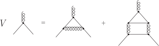
While the early bootstrap progamme of Refs. [195, 196] and [197] in a strictly three dimensional scalar theory was used as a seed idea for the modern numerical bootstrap revolution, it also provided the basis for an analytic bootstrap using the large expansion in arbitrary dimensions. This was developed originally in Ref. [36] for the universality class containing (2.1) and to avoid confusion will be referred to as the large conformal bootstrap. The beauty of the construction [36] is that the critical exponent of the field was determined as a function of to analytically†††We note that in Ref. [36] there was a typographical error in one term of the expression for which was corrected in Ref. [214] and noted also in Ref. [57] which was the six loop evaluation of the anomalous dimension of in theory.. At criticality an algebraic consistency equation can be deduced from the vertex function where is an amplitude, and are the field exponents. The quantities and are regularizing parameters which regularize divergences associated with vertex subgraphs [195, 196, 197] and are effected by shifting the exponents of the fields of two of the external legs. This is similar to (4.43) and both are indicative of the fact that this approach using the critical point large formalism is also in effect perturbation theory in the vertex anomalous dimension. The leading order consistency equation for the vertex function is graphically illustrated in Fig. 9 with the higher order graphs given in Ref. [36]. In Fig. 9 like Fig. 8 there are no self-energy corrections on the propagators. At the Wilson-Fisher fixed point the asymptotic scaling forms of the propagators are used and include the anomalous dimension in the exponent. This quantifies the contribution from the virtual propagator corrections so that including decorations on lines would overcount. However there is a difference between Fig. 9 and Fig. 8 which is in part the essence of the bootstrap. This is that the vertices are also dressed which is what in effect is represented by the dot at each vertex. Indeed the vertex expansion of Fig. 9 is in terms of primitive graphs with no vertex subgraphs within the ordering of the expansion by . We recall that this means that a line counts a factor of and a closed loop counts .
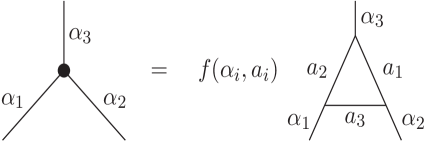
The evaluation of the vertex function using the primitive graphs as the basis for the large conformal bootstrap formalism [36, 193, 194, 195, 196, 197] relies on the fact that the dot of the vertex is defined to be what is termed a Polyakov conformal triangle [36, 193, 194]. This is defined graphically in Fig. 10 in coordinate space representation for general scalar propagators with exponents . The dotted vertex is replaced by a one loop graph where the exponents of the internal lines, , are chosen so that each of the new vertices connecting to an external line are unique in the sense of Refs. [34, 35] and [196]. In other words the sum of the exponents of the three lines joining at a vertex is equal to the spacetime dimension. For Fig. 10 this means that
| (7.92) |
These conditions also apply to the situation when the vertex regularizing parameters decorate the overall primitive graph of the large bootstrap expansion. In Appendix A we have discussed at length the derivation and properties of unique vertices as well as their power in computing massless scalar and fermion Feynman graphs particularly. With the uniqueness property the one loop integral of Fig. 10 can be related to the original vertex with the proportionality, , reflecting the exponent dependence. In practical terms for (2.1) will involve and . For the conformal triangle application to the bootstrap the key point is that the replacement of a dressed vertex by Polyakov’s conformal triangle means the complicated -point graphs of Fig. 9 can be evaluated using conformal methods [36]. In particular if one applies a conformal transformation of the form of (5.64) to each of the variables of a graph in Fig. 9 then the choice of the internal lines of (7.92) for all vertices means that the -point vertex graphs immediately collapse to -point integrals. These have structural similarities to the graphs of Fig. 8 and similar techniques which were used to evaluate those graphs can be applied to the graphs of the bootstrap equations. For instance given that there are three different possible ways of applying a conformal transformation to a -point graph this gives enough information to determine the graphs of Fig. 9 to the next order in as discussed in Ref. [36]. This is necessary as part of the process to find an expression for .
These tools provide the value of the vertex function when the vertex regularizing parameters and are nonzero. Once is available at a specific order in one has to extract the value for at that order. Like the earlier -point construction to find the function contains several variables which aside from are and . The value of the latter is only required at one order less than that of . Therefore three equations are needed in order to be able to solve for the value of . The formalism to derive these was presented in Ref. [197], which introduces the regularization procedure, and are [36]
| (7.93) |
where is a function that depends on the and . In practice its value is not needed since it can be eliminated to produce
| (7.94) |
which is sufficient to find in -dimensions once the explicit expansion for is available from the first equation of (7.93). The explicit evaluation of all the contributing graphs is an exercise separate from the formal construction of the key equations. In light of the earlier sections on relating large exponents in the -dimensional universal theory to the perturbative renormalization group functions in various critical theories, it is worth emphasising not only how much information is contained in of Ref. [36] and its usefulness for recent six and seven loop computations [57, 58, 59] but how far ahead of its time was the result. Moreover it represents the limit that has been achieved so far in terms of orders of expansion in in this or any other model. Similar results have been determined for (2.2) and variations on the core Gross-Neveu Lagrangian where there are extra symmetries such as chiral symmetry. For several relevant articles for (2.2) see, for example, Refs. [169] and [172].
7.2 Conformal field theory connections
While our large critical exponent focus has in part been in relation to the connection with field theories in integer dimension spacetimes, the fact that information is available on exponents for a continuous value of the spacetime dimension is of interest due to overlap with other techniques. At this point we have to stress that we are not suggesting the rigorous existence of field theories in noninteger dimensions in general. However as an aside we note that the class of scalar field theories which has one self-interaction of the form has a critical dimension of as noted in Ref. [215], for instance. For as well as for the critical dimension is rational and the latter case has an application in condensed matter physics [216, 217]. These situations aside in the universal theory context where a core interaction dictates the properties of the underlying fixed point one has in principle data on that theory for all . For instance, it is possible to plot the behaviour of the critical exponents to or in the case of as well as and as a function of as illustrated in Ref. [159]. In the case of critical exponents for several universality classes based on the Gross-Neveu-Yukawa structure their qualitative behaviour matches closely with studies using the functional renormalization group, which we noted earlier.
A specific example where this can be seen clearly is for the chiral Heisenberg-Gross-Neveu model which is believed to be in the universality class of a phase transition in graphene [218, 219, 220, 221]. In Ref. [218] the behaviour of exponents , and are plotted as a function of in Figs. , and of that article with the corresponding large plots given in Fig. of Ref. [221]. Both sets of graphs are for the case of . Similar analyses have been carried out for the original Ising Gross-Neveu model of (2.2) but the behaviour of the exponents in -dimensions is not the same as for the chiral Heisenberg-Gross-Neveu case. However the separate results from the large and functional renormalization group methods are effectively parallel and certainly in qualitative agreement.
One consequence is that there are several analytic ways now of estimating exponents in three dimensions which is the spacetime of interest. While for many years the original expansion of exponents in either two or four dimensions offered a way of extracting estimates in three dimensions after resummation, nowadays one has to have a large number of loop orders in order to be competitive with say Monte Carlo results. For example, the detailed and comprehensive study of Ref. [58] to extract exponent estimates in three dimensions from six loop theory represents the current state of the art in terms of summation. It has yet to be extended to the seven loop case of Ref. [59]. Indeed it has reopened the debate concerning the asymptotic behaviour of the strictly four dimensional -function at large loop order which is discussed in Ref. [222]. For instance, early ideas in this direction [223, 224, 225, 226, 227, 228, 229, 230] were unable to benefit from the high loop order data that has been revealed in more recent years. In light of the possibility of reliably studying field theory for arbitrary the information contained in the expansion can be viewed in a new way. Again this has been examined in the case of the Ising Gross-Neveu model [231]. The approach is to collect the information contained in the expansion of the two theories in the universality class near two and four dimensions and construct a Padé approximant to the exponent in -dimensions. For the Ising Gross-Neveu model of (2.2) a matched approximant has been precisely constructed from the four loop renormalization group functions of (2.2) and (5.70) which have been computed over several years [158, 160, 232, 233, 234]. Moreover the behaviour of the three highlighted exponents in qualitatively matches that from the other two techniques. Indeed the comprehensive analysis of Ref. [231] has demonstrated that the combination of the data from the various approaches can give accurate three dimensional estimates similar to using Monte Carlo simulations. The latter by the very nature of the technique is strictly three dimensional.
While we have noted the complementary aspects of the large method with other techniques such as the perturbative expansion and the functional renormalization group technique the first two are in effect different views of the same underlying technique. By contrast the functional renormalization group deploys fundamental aspects of the renormalization group to gain structural data on the theory. It is nonperturbative in nature. However in being able to study field theories with the spacetime dimension not fixed to be an integer value it is also possible to carry out large studies with the functional renormalization group method. Early work in this direction can be found in Refs. [235] and [236]. However in recent years several aspects of that work has come into question since results apparently contradict results from other methods. An example of where this was observed is Ref. [176] where scalar models were studied. The resolution was subsequently provided in Ref. [177] where the assumptions in the development of the core functional renormalization group equations in the large limit were re-examined.
8 Discussion
In this review we have endeavoured to give a balance between background to the development of the large expansion in quantum field theories relating to particle physics and more recent directions. In the main in the latter case this has concerned the large critical point formalism of Refs. [34, 35] and [36] although there are other large approaches which we have not discussed at length [237, 238]. The main feature of the critical point approach is the use of the underlying universal field theory living at the -dimensional Wilson-Fisher fixed point. This allows one to compute renormalization group invariant data through the -dimensional critical exponents. The current viewpoint is that the information derived from these complement analyses from other methods. It is perhaps in this general context that one ought to view the overall technique. In studying problems of interest such as phase transitions, there are a variety of techniques such as the expansion or perturbation theory, conformal bootstrap and the functional renormalization group which can equally be used as investigation tools. However each in their own way and approximation computes data on the same quantity. Rather than compete the current movement is now towards pooling that information in order to improve the overall picture. This has been evident in the exponent estimates in the Gross-Neveu analysis of Ref. [231] where there is a hope that equivalent reliable precision will be obtained for similar and other theories. In this context we have focused throughout on two key theories which are the nonlinear sigma model and the Gross-Neveu model as well as their four dimensional counterparts which are theory and the Gross-Neveu-Yukawa models respectively. This is partly because not only are their perturbative renormalization group functions known to very high loop order but the leading three terms of the large critical exponents are available. With recent activity in critical field theories revealing the concept of emergent symmetries where apparently different theories can be connected at one fixed point, there is now a need to develop the critical point large method to a new set of models.
One such model is the model which is a generalization of (2.1) where there is a gauge field. This has been studied over many years in the large expansion in different contexts. See Refs. [142, 144, 239, 240, 241, 242, 243, 244, 245] and [246] for several instances. At present there is interest in the critical properties of the model in three dimensions. One example of this is that for a specific value of it has connections with a possible duality [247, 248, 248, 250, 251] in an extension of (2.2) where a QED sector is appended. To probe the duality further requires data on the critical exponents to high precision for the model side of the equivalence. In this context there are only a few leading order large critical point studies [142, 144] with no exponents known in -dimensions. In principle the necessary formalism is available to carry out the computations to . However such calculations will be tedious due to the presence of the gauge field. As is discussed in the Appendices the useful calculational technique of conformal integration for scalar and scalar-Yukawa type vertices has no parallel for a scalar-gauge or fermion-gauge vertex. While this can be circumvented by methods reviewed in the Appendices for practical purposes of determining specific integral values, it is perhaps indicative of the potential conflict between gauge and conformal symmetry indicated briefly earlier and in Ref. [252]. For instance, this limitation of conformal integration in a gauge sector would suggest that the development of the Polyakov triangle and conformal vertex for a gauge theory is technically difficult if not impossible. Moreover it is not clear if there are obstructions to applying the modern manifestation of the conformal bootstrap to gauge theories for related reasons. That aside in Ref. [147] an attempt was made to develop the basic equations introduced in Ref. [197] similar to (7.93) for a gauge theory but these were not placed in the large context. While we have noted this in the context of the model which is a scalar theory the same potential limitations would apply to any extension to QED or QCD. For the other major symmetry of field theoretic interest, supersymmetry, the large critical point formalism can be applied without any deep problems. For instance exponents in the supersymmetric nonlinear sigma model have been computed [253, 254]. Indeed early large work on this specific model [255, 256, 257, 258] and the extension [259, 260] revealed a mine of very rich properties due to the underlying supersymmetry. In the latter case the critical point formalism has again only been applied at leading order [261, 262] in . The relation of large results to the understanding of lattice computations can also be found in Refs. [83] and [263].
Finally we note that any review of a topic while there is still development activity in the area can merely represent a brief snapshot of the subject before it is superseded by new breakthroughs. Although the large methods in general have served the development and understanding of quantum field theories well over a period of half a century they can only ever be a complementary tool to our overall understanding of the part of Nature we wish to describe. However at this particular point exciting new ideas are being examined which we have alluded to such as the hope that gravity can be finally unveiled through Weinberg’s asymptotic safety vision [126] as well as the potential of emergent symmetries to give insight into the theory which lies beyond the Standard Model.
Acknowledgments
This work was supported in part by the STFC Consolidated Grant ST/L000431/1 and a DFG Mercator Fellowship. Also the author has great pleasure in alphabetically thanking Dr. J. Babington, Dr. J.M. Bell, Prof J. Blümlein, Dr. D.J. Broadhurst, J. Hackett, Dr. J.R. Honkonen, Prof I. Jack, Dr. H. Kissler, Prof D. Kreimer, Prof S. Moch, Prof A.J. Niemi, Prof H. Osborn, Dr. E. Panzer, Dr. M.M. Scherer, Dr. R.M. Simms, Dr. S. Teber and Dr. J.A.M. Vermaseren for many valuable discussions, encouragement, interest and support over either early, many or recent years on foundational aspects of material in this article. The hospitality of LPTMC, Sorbonne University, Paris and the Mathematical Physics Group at Humboldt University, Berlin, where part of the work was carried out, is also gratefully acknowledged. The figures were prepared with Axodraw [264] and various calculations could not have been achieved over the years without the symbolic manipulation language Form [265, 266].
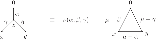
Appendix A Computational methods
As the large critical point formalism involves (massless) propagators with nonunit powers unlike conventional perturbation theory the well-developed and standard techniques to evaluate Feynman integrals cannot always be applied. By this we mean analytic methods ranging from the early introduction of integration by parts [267, 268, 269] and the Gegenbauer polynomial approach [270] to the Mellin-Barnes representation of propagators [271, 272]. The success of several of these have led to computer algebra packages to determine the poles and finite parts of three, four and higher loop Feynman graphs. These include Mincer [273, 274] and its four loop successor Forcer [275, 276], which are efficient tools in the main for evaluating massless -point functions in four dimensional theories, as well as the packages which were developed to implement the systematic integration by parts algorithm of Laporta [277] such as Reduze [278, 279], Fire [280], Litered [281, 282], Air [283] and Kira [284]. While the Laporta method has the benefit of handling huge numbers of Feynman integrals to complete the evaluation of a Green’s function it requires the explicit values of what is termed master integrals for the final stage. This is where other techniques are relevant such as Mellin-Barnes and Schwinger parameter representations of Feynman graphs. Packages for the implementation of these are available such as Mb [285] and Hyperint [286]. A recent comprehensive review of these techniques has been provided in Ref. [287] while we will focus on another method almost exclusively used for the large critical point technique.
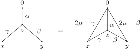
While these and other techniques are more than valuable in pushing back our conventional perturbative knowledge of the renormalization group functions of many theories to very high loop order, there is another method which is central to the class of Feynman diagrams which arise in the critical point large approach. It is termed conformal integration or uniqueness and was introduced in Ref. [196] specifically for three dimensions. Thereafter it was extended to -dimensions in Refs. [34] and [35] as the conditions when the uniqueness method can be applied are naturally satisfied for the large calculations at the -dimensional Wilson-Fisher fixed point of the scalar and fermion theories we have discussed. While this is the main direct application of conformal integration, it has been used in certain cases for evaluating finite integrals in perturbation theory. For instance, in Refs. [288] and [289] two loop finite massless off-shell master -point integrals were evaluated in terms of the polylogarithm function. In that particular computation the master integral was analytically regularized and the uniqueness rule applied after an integration by parts. Moreover there is a comprehensive introduction to the application of uniqueness to very high loop order integrals in the lectures of Ref. [290]. Details are provided there on some of the more technical developments of the method. Other sources can be found in Refs. [55, 291, 292] and [293] and [294]. In the case of Ref. [291] it was used to determine the value of the four loop massless -point zigzag graph for the final remaining analytic number required for the five loop -function of theory in four dimensions [55]. This was subsequently extended to five loops for the case [56] as well as six [57] and seven [58] loops. These were all for the scheme. The latter two evaluations used the more modern approaches bannered under the heading of applications of algebraic geometry. To be more concrete the rule for integrating over what is called a unique vertex is given in Fig. 11. To summarize when the sum of the exponents of three propagators is equal to the spacetime dimension [35] then the integration over the vertex coordinate can be carried out‡‡‡In this Appendix we use as a coordinate which is not to be confused, for instance, with the combination of amplitudes used in (4.42).. This rule is also sometimes referred to as the star-triangle rule.

There are various ways of verifying the relation of Fig. 11. One is to carry out the explicit integration over using Feynman parameters which produces a one parameter integral involving a hypergeometric function dependent on arbitrary , and . The final integration cannot be completed in general for the three independent values of the exponents in general. However when the uniqueness condition [34, 35]
| (A.95) |
is satisfied the hypergeometric function collapses to a simple form allowing the final one parameter integration to proceed. When a vertex satisfies this criterion it is called a unique vertex. By contrast when the sum of the exponents on the lines comprising a triangle sum to then it is termed a unique triangle and can be replaced by a unique vertex. This is evident from the right hand side of the equation in Fig. 11. A more elegant way of deriving the result is to apply the conformal transformation of (5.64). For example, using
| (A.96) |
and similar mappings for the other coordinates gives
| (A.97) |
where the Jacobian associated with the measure is indicated in the second equation. The application of (A.97) to the integral on the left side of the equation in Fig. 11 is illustrated in Fig. 12 where for shorthand we have set and used the top external leg as the reference origin for the transformation. Choosing the origin at one of the other external points would lead to a different graph topology under a conformal transformation but the same overall uniqueness relation. The graph on the right hand side of the equation in Fig. 12 cannot be completed for arbitrary values of the exponents. However if the exponent of the propagator is zero or a nonnegative integer then the resulting simple integration over the -vertex can be completed. When then the result of Fig. 11 emerges. In the case when where is a positive integer then a more involved rule emerges [214, 295] which is called steps from uniqueness. The one step case is given in Fig. 13. A complementary rule can be derived from this case by taking its Fourier transform [214]. It is illustrated in Fig. 14 and corresponds to a one step from unique triangle. Generalizations of both rules are available in Refs. [156] and [214] with a mixed rule given in Ref. [290].
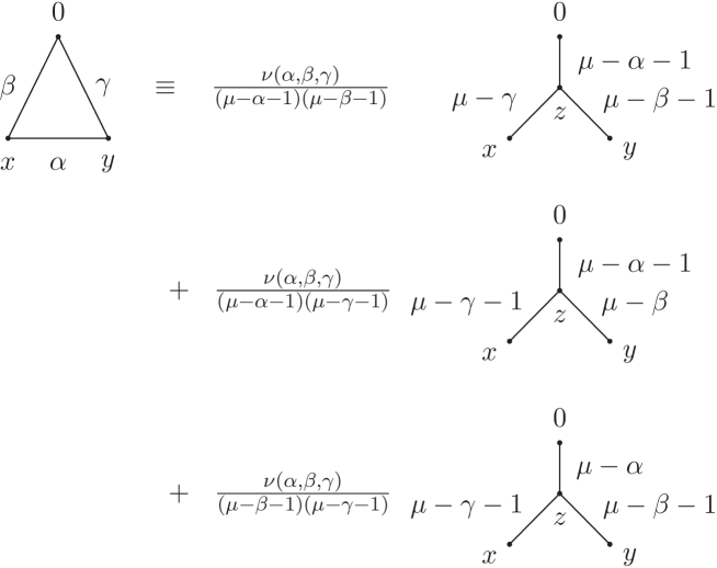
One benefit of the rule of Fig. 13 is that one can derive relations between different Feynman integrals. For computations even though there are high loop graphs to be determined for the skeleton Schwinger-Dyson equations in the detailed evaluation the more intractable ones reduce to two loop scalar self-energy graphs with nonunit propagator exponents. To extract the required value, if it cannot be carried out in a simple direct way, necessitates a type of large Laporta algorithm where the integral is manipulated to what is now termed as master integrals. While the Laporta algorithm used for explicit perturbative computations is systematic and encoded in symbolic manipulation computer programmes, the situation for the large graphs has yet to be systematized. This is partly because there is no systematic way of finding a concrete termination point in the algorithm. For perturbative integrals with unit exponent propagators integration by parts can nullify this power on one propagator which reduces the graph to one of a lower topology. Hence, in principle, it is easier to determine. With nonunit exponents in the large critical point approach it is rare that integration by parts or the approach we will review here will reduce an integral to a lower topology. Instead what one has to effect is the reduction of a graph to a situation where a vertex or a triangle becomes unique whence one can carry out an evaluation. An example of this is given in the next section.
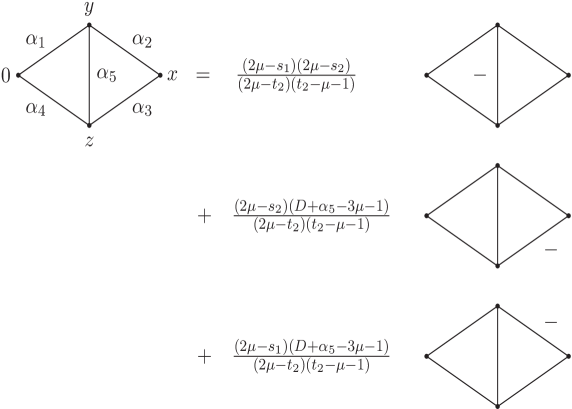
An example however of the type of relations which be derived using the one step from uniqueness [295, 296] is illustrated in Fig. 15 where are arbitrary exponents. The distribution of these exponents on the propagators in the graphs on the right hand side of the equation are the same as the corresponding one on the left except where there is a minus sign. In that case the power of the exponent is reduced by unity. The parameters appearing in the coefficients of the graphs in Fig. 15 correspond to those introduced in Ref. [35] and are related to the . The full set are
| (A.98) |
As an aside the general properties and structure of the two loop self-energy graph of the left hand side of the relation in Fig. 15 has now been well-established. For instance, an early investigation of its full set of symmetries was provided in Refs. [297] and [298] while the all orders expansion of the case when where was given in Ref. [299] having built on earlier high order expansions [35, 139] for instance. The result of Ref. [299] established that the series expansion only contains multiple zeta values. The relation of Fig. 15 is not the only such relation as one can derive similar ones. However, one benefit it has is that it reduces the sum of exponents at least at one vertex or for one triangle. So it is akin to the integration by parts reduction that is at the heart of the Laporta algorithm. Moreover the associated prefactors are not singular at any integers as is the case in similar relations. This is evident in the more complete set of these relations that have been listed in the Appendix of Ref. [300].
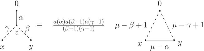
While the focus of the conformal integration has been on scalar vertices the rules can be generalized to other cases. For instance, rules for vertices with tensor structure involving the vectors of the three propagator meeting at in Fig. 11 have been given in Refs. [156, 293, 301, 302] and [303]. Another direction is the construction of a uniqueness rule for vertices involving fermions which can be applied to Yukawa type theories. The basic unique vertex for the Gross-Neveu model was provided in Ref. [146] and shown in Fig. 16. Due to the presence of fermion propagators the criterion for integration differs from that of the purely scalar case in that the sum of the exponents of the propagators meeting at a vertex have to be one higher than the spacetime dimension. The derivation of this rule can be carried out in either of the two ways indicated for the full scalar vertex. In order to use the conformal transformation approach the rules of (A.97) imply
| (A.99) |
where there are two ways of writing the result of the transformation. One is more useful than the other depending on the structure of the neighbouring propagator. So for example when one is dealing with a scalar-fermion vertex whose Feynman rule does not involve a -matrix then applying a conformal transformation to successive strings of numerators which appear in a fermion propagator we have
| (A.100) |
This implies that transforming the vertex on the left side of that shown in Fig. 16 the internal propagator structure is preserved. Again we have chosen the origin for the conformal transformation to be at the top of the scalar propagator. Under the transformation it is the exponent of this line which provides for the definition of the uniqueness condition similar to that shown in Fig. 12. The denominator factors in (A.100) lead to the appearance of unity in the condition for a scalar-fermion uniqueness condition which is . While the rule of Fig. 16 is extremely useful for large critical point computations in the Gross-Neveu universality classes, it can be generalized to steps away from uniqueness similar to the rule of Fig. 13. The case of is given in Fig. 17 where
| (A.101) |
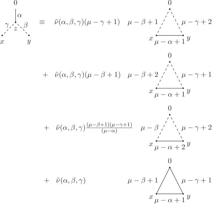
Although the two main uniqueness rules for a pure scalar and Yukawa vertices have proved to be of significant benefit to evaluating the underlying Feynman graphs needed for high order large computations the extension to gauge theories is not straightforward. By this we mean the usual gluon-quark vertex of QCD rather than the vertex of a scalar gauge theory. This is because a technical complication arises due in essence to the -matrix structure in the vertex. In addition the propagator of the gauge field of (5.52) in coordinate space is comprised of two terms. Although the first is not unlike the scalar propagator the second part is in effect a rank tensor. Ignoring the -matrix of the fermion propagator form of (5.52) then in that case one is dealing with a rank tensor. It is this in effect which was responsible for the Yukawa vertex having a uniqueness condition requiring the exponents at the vertex to sum to in contrast to the rank case of . Therefore on these grounds one would expect the uniqueness condition for a gauge-fermion vertex for a gauge field in a general gauge to be . To apply such a rule to large gauge theories, however, one would require the exponent sum to be on dimensional grounds given in (5.55). However it turns out that there is a situation where for a certain value of the gauge parameter this uniqueness condition could be replaced by one with a smaller value such as which would then be of potential use. For it to be useful for practical purposes though, it should not produce an evaluation where the original gauge is not preserved. A detailed study of conformal integration for the specific case of a gauge-fermion vertex has been discussed at length in Refs. [301, 302] and [303]. In addition the rule for a general vertex with tensor structure is summarized in Refs. [156] and [293]. In Refs. [301, 302] and [303] the special case for a unique gauge-fermion vertex for a value of the sum of the vertex exponents being lower than above the spacetime dimension was discussed. This is the case when either (5.67) or (5.68) is satisfied. In other words the asymptotic form of the gauge field propagator is proportional to . The reason for the simplification can be seen by applying a conformal transformation to the gauge-fermion vertex in the same way as in (12) when the gauge field propagator involves . After the transformation part of the string of -matrices involves
| (A.102) |
Using the Clifford algebra of the -matrices produces . For any other gauge this simplification would not happen. Therefore to complete the integration the analogous exponent , similar to that in previous cases, is set to zero which means that the uniqueness condition in this case is the same as the scalar-fermion case. However the -integration has to be completed and this is not similar to the simpler vertices as it involves a rank tensor. Consequently one cannot write the integral under this uniqueness condition as a triangle involving the original propagators of the vertex nor indeed as one term. Therefore we have not provided a graphical representation of the rule for this particular gauge choice but it can be found in Ref. [303] as well as in Ref. [150, 156]. Another way of viewing the lack of a uniqueness rule analogous to those of (12) and (16) for a general gauge field propagator is that under a conformal transformation the gauge which one is carrying out the calculation in is not preserved. While this effectively rules out applying direct conformal transformations on large graphs in a gauge theory, the underlying Feynman graphs themselves can still be evaluated using indirect conformal methods. By this we mean the tedious decomposition of the graph into the constituent scalar Feynman integrals by taking the spinor traces and then using the scalar vertex uniqueness rule as well as integration by parts on these individual integrals.
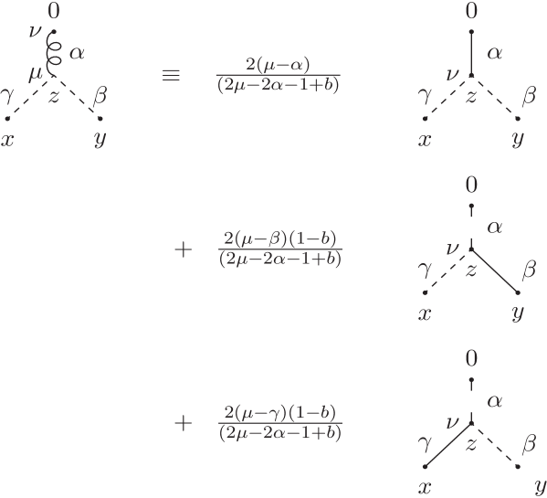
While such an approach is in principle not problematic one can still use properties of the gauge-fermion vertex at the start of a large gauge theory integral evaluation. Aside from the rule provided in Refs. [301, 302] and [303] another rule for the gauge vertex can be constructed and partially simplifies the complications stemming from the second term of the gauge propagator in (5.52). This is achieved by using integration by parts on the second term inside the coordinate space representation of the vertex. The rule is illustrated in Fig. 18 where the curly line corresponds to the gauge field propagator for nonzero gauge parameter of (5.52). We have indicated the location of the Lorentz indices and . When it is adjacent to the vertex it indicates the -matrix contracted with one of the indices on the gauge propagator. When it appears at the outer end of this type of propagator it contracts the -matrix of the adjacent gauge-fermion vertex. For the final two vertices the Lorentz index is the label of the vector which is denoted by the long dash line. The other dashed line corresponds to a standard fermion propagator. The benefit of these final two graphs is that the -matrix structure is simpler whereas the first term is trivial in the sense that it is the Feynman gauge term of the left side of the equation.
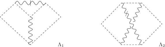
Appendix B Examples of integral evaluation
In this section we give several examples of how the rules of the previous section are applied in practical situations. In particular we will discuss the various steps in integrating two graphs which occur in the computation of the exponent from Ref. [171] which is related to the critical slope of the -function of (2.2) at . These are illustrated in Fig. 19 where the tick line on a field indicates the correction to scaling term of the corresponding asymptotic scaling form of the propagator given in (5.62). For instance for the two dimensional -function the leading term of the correction exponent is .
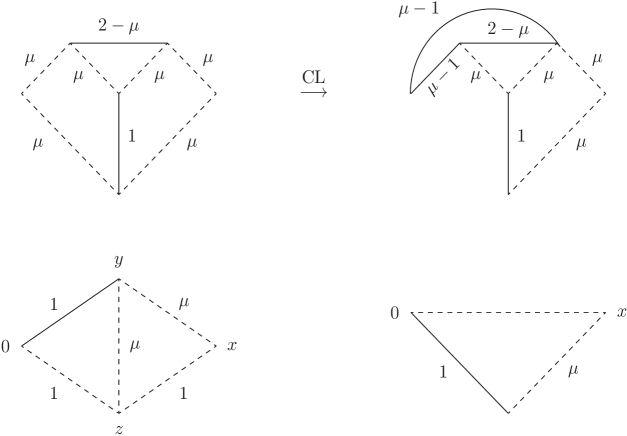
First we concentrate on the sequence of steps to evaluate which are given in Fig. 20. The starting point is the graph of the top left where we have included the exponents of the respective lines where there is a single trace over the -matrices. In this coordinate space representation there are four rather than three integrals to compute since there are four internal vertices to integrate over. While this may sound daunting the number can be reduced quickly by several of the techniques mentioned previously. First if we define the coordinate of the left external vertex as the origin then applying the conformal transformations (A.97), (A.99) and (A.100) on the graph produces the graph of the top right of Fig. 20. This transformation is denoted by CL in Fig. 20 meaning conformal left [35]. In effecting this there is still a trace over the fermion lines even though the graph shows a noncontinuous string of fermions. The reason for the break is that in rules (A.99) and (A.100) introduce pieces such as which drop out of the trace and alter the power of the associated propagator. In certain instances a line can disappear as the sum of the exponents after all aspects of the transformations have been taken into account is zero. This is the case for one such line. While there are still four vertices to be integrated over in the resulting graph two can be carried out immediately. One is the boson fermion chain where the bottom vertex is integrated over. The other is the unique triangle which has appeared involving the bosonic propagator with exponent . Carrying out this integration using the rule of Fig. 11 in reverse produces an integral which in effect is another chain in the coordinate space representation of Fig. 7. By this we mean that one link in the chain is the main integral itself which is some -dependent function times a propagator with power and the propagator with power stemming from the propagator with the correction to scaling. The power arises from the dimensionalities of the propagators as well as that of the integration measure. The upshot is that after these two integrations the bottom left graph of Fig. 20 emerges. Here the trace is . The final integration is over the -vertex as this is unique from the rule of Fig. 16. Applying it and noting that produces the final chain integral of the graph at the bottom right of Fig. 20. While this describes the algorithm to evaluate account has to be kept of the factors associated with each step. Doing so produces
| (B.103) |

The second case we consider is the nonplanar graph of Fig. 19 denoted by . It corresponds to the top left graph of Fig. 21 where the exponents are included. Again there are four integrations to be performed which can be reduced to three by first applying the uniqueness rule to the lower left vertex and apply the rule of Fig. 16. Applying a conformal left transformation to the resultant graph produces the graph at the top right of Fig. 21 which contains a unique triangle. Implementing the unique scalar vertex relation of Fig. 11 produces the graph of the bottom left in Fig. 21 after several chain integrals. The last step is to apply the transformation to the right hand external vertex of this graph. While the details of this rule were introduced in Ref. [35] for a purely scalar two loop self-energy this transformation has a parallel for the scalar-fermion unique vertex of Fig. 11. The upshot is the graph at the bottom left of Fig. 21. The steps described so far are not dissimilar to those discussed for and we have given a brief summary for this reason. The key point here is that the final evaluation differs in the last step from that for . In the graph the trace is and we have noted this since it has to be evaluated at the next step. This creates a technical problem due to a singularity in several of the resulting scalar integrals deriving from the exponent of the central propagator. When a scalar line has an exponent where is an integer and then the associated function for this exponent, , will be divergent.
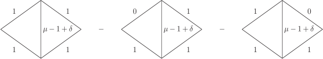
To circumvent the singularity after taking the trace a temporary regularization is added to the exponent of this line which is denoted by in Fig. 21. In this and other cases where a temporary regularization is introduced to overcome hidden singularities the location where the regulator is placed is not unique. Moreover an appropriate choice is one where there is no obstruction to subsequent integration and the intermediate or temporary regularizing parameter must be located on the analogous lines in each of the graphs. For instance, it is not difficult to imagine placing it in such a way that a nonproblematic unique vertex within a graph ceases to be unique for a nonzero . Writing
| (B.104) |
simplifies the earlier trace. The integral corresponding to the first graph of (B.104) is a set of simple chain integrations where the initial one produces a divergence. Overall it gives
| (B.105) |
where the singularity is in the third argument of the first -function. Taking the trace in the second term of (B.104) produces the three graphs of Fig. 22. The first is finite while the final two are equivalent under reflection. The value for one of these is
| (B.106) |
Summing the two contributions from (B.105) and (B.106) in the context of (B.104) gives
| (B.107) |
and hence the temporary regularization can be safely lifted. The value of the remaining finite graph was given in Ref. [35] so that the sum of all contributions to ultimately gives
| (B.108) |
References.
- [1] J.S. Schwinger, Phys. Rev. 73 (1948), 416.
- [2] A. Petermann, Helv. Phys. Acta 30 (1957), 407.
- [3] S. Laporta & E. Remiddi, Phys. Lett. B379 (1996), 283.
- [4] T. Kinoshita & M. Nio, Phys. Rev. D73 (2006), 013003.
- [5] T. Aoyama, M. Hayakawa, T. Kinoshita & M. Nio, Phys. Rev. D77 (2008), 053012.
- [6] T. Aoyama, M. Hayakawa, T. Kinoshita & M. Nio, Phys. Rev. Lett. 109 (2012), 111807.
- [7] D. Hanneke, S. Fogwell & G. Gabrielse, Phys. Rev. Lett. 100 (2008), 120801.
- [8] D. Hanneke, S. Fogwell Hoogerheide & G. Gabrielse, Phys. Rev. A83 (2011), 052122.
- [9] P.A. Baikov, K.G. Chetyrkin & J.H. Kühn, Phys. Rev. Lett. 118 (2017), 082002.
- [10] F. Herzog, B. Ruijl, T. Ueda, J.A.M. Vermaseren & A. Vogt, JHEP 1702 (2017), 090.
- [11] T. Luthe, A. Maier, P. Marquard & Y. Schröder, JHEP 1710 (2017), 166.
- [12] K.G. Chetyrkin, G. Falcioni, F. Herzog & J.A.M. Vermaseren, JHEP 1710 (2017), 179.
- [13] D.J. Gross & F.J. Wilczek, Phys. Rev. Lett. 30 (1973), 1343.
- [14] H.D. Politzer, Phys. Rev. Lett. 30 (1973), 1346.
- [15] W.E. Caswell, Phys. Rev. Lett. 33 (1974), 244.
- [16] D.R.T. Jones, Nucl. Phys. B75 (1974), 531.
- [17] O.V. Tarasov, A.A. Vladimirov & A.Yu. Zharkov, Phys. Lett. B93 (1980), 429.
- [18] T. van Ritbergen, J.A.M. Vermaseren & S.A. Larin, Phys. Lett. B400 (1997), 379.
- [19] M. Czakon, Nucl. Phys. B710 (2005), 485.
- [20] G. ’t Hooft, Nucl. Phys. B72 (1974), 461.
- [21] A.A. Migdal, Phys. Rept. 102 (1983), 199.
- [22] B. Lucini & M. Panero, Phys. Rept. 526 (2013), 93.
- [23] C. Wetterich, Nucl. Phys. B352 (1991), 529.
- [24] C. Wetterich, Phys. Lett. B301 (1993), 90.
- [25] T.R. Morris, Int. J. Mod. Phys. A09 (1994), 2411.
- [26] K.G. Wilson, Phys. Rev. B4 (1971), 3174.
- [27] F.A. Dolan & H. Osborn, Nucl. Phys. B599 (2001), 459.
- [28] R. Rattazzi, V.S. Rychkov, E. Tonni & A. Vichi, JHEP 0812 (2008), 031.
- [29] R. Rattazzi, V.S. Rychkov & E. Tonni, JHEP 0812 (2008), 031.
- [30] S. El-Showk, M.F. Paulos, D. Poland, S. Rychkov, D. Simmons-Duffin & A. Vichi, Phys. Rev. D86 (2012), 025022.
- [31] F. Kos, D. Poland & D. Simmons-Duffin, JHEP 1406 (2014), 091.
- [32] D. Poland, S. Rychkov & A. Vichi, arXiv:1805.04405 [hep-th].
- [33] D. Poland & D. Simmons-Duffin, Nature 12 (2016), 535.
- [34] A.N. Vasil’ev, Yu.M. Pismak & J.R. Honkonen, Theor. Math. Phys. 46 (1981), 104.
- [35] A.N. Vasil’ev, Yu.M. Pismak & J.R. Honkonen, Theor. Math. Phys. 47 (1981), 465.
- [36] A.N. Vasil’ev, Yu.M. Pismak & J.R. Honkonen, Theor. Math. Phys. 50 (1982), 127.
- [37] K.G. Wilson, Phys. Rev. B4 (1971), 3184.
- [38] K.G. Wilson, Phys. Rev. Lett. 28 (1972), 548.
- [39] K.G. Wilson & M.E. Fisher, Phys. Rev. Lett. 28 (1972), 240.
- [40] K.G. Wilson, Phys. Rept. 12 (1974), 75.
- [41] R. Abe, Prog. Theor. Phys. 49 (1973), 1877.
- [42] A.J. Bray, Phys. Rev. Lett. 32 (1974), 1413.
- [43] Y. Okabe, M. Oku & R. Abe, Prog. Theor. Phys. 59 (1978), 1825.
- [44] Y. Okabe, M. Oku & R. Abe, Prog. Theor. Phys. 60 (1978), 1277.
- [45] Y. Okabe & M. Oku, Prog. Theor. Phys. 60 (1978), 1287.
- [46] I. Kondor & T. Temesvári, J. Physique Lett. 39 (1978), 99.
- [47] Y. Okabe & M. Oku, Prog. Theor. Phys. 61 (1979), 443.
- [48] I. Kondor, T. Temesvári & L. Herényi, Phys. Rev. B22 (1980), 1451.
- [49] S.-K. Ma, Phys. Rev. A7 (1973), 2172.
- [50] E. Brézin, J.C. Le Guillou, J. Zinn-Justin & B.G. Nickel, Phys. Lett. A44 (1973), 227.
- [51] A.A. Vladimirov, D.I. Kazakov & O.V. Tarasov, Sov. Phys. JETP 50 (1979), 521.
- [52] F.M. Dittes, Yu.A. Kubyshin & O.V. Tarasov, Theor. Math. Phys. 37 (1978), 879.
- [53] K.G. Chetyrkin, A.L. Kataev & F.V. Tkachov, Phys. Lett. B99 (1981), 147 [Erratum: Phys. Lett. B101 (1981), 457].
- [54] K.G. Chetyrkin, S.G. Gorishniy, S.A. Larin & F.V. Tkachov, Phys. Lett. B132 (1983), 351.
- [55] D.I. Kazakov, Phys. Lett. 133B (1983), 406.
- [56] H. Kleinert, J. Neu, V. Schulte-Frohlinde, K.G. Chetyrkin & S.A. Larin, Phys. Lett. B272 (1991), 39 [Erratum: Phys. Lett. B319 (1993), 545].
- [57] D.V. Batkovich, K.G. Chetyrkin & M.V. Kompaniets, Nucl. Phys. B906 (2016), 147.
- [58] M.V. Kompaniets & E. Panzer, Phys. Rev. D96 (2017), 036016.
- [59] O. Schnetz, Phys. Rev. D97 (2018), 085018.
- [60] S. Coleman, , in Pointlike structures inside and outside hadrons, ed. A. Zichichi (Plenum Press, New York, 1982) p. 739.
- [61] S. Coleman, Aspects of symmetry: selected Erice lectures, (Cambridge University Press, Cambridge, UK, 1985).
- [62] M. Moshe & J. Zinn-Justin, Phys. Rept. 385 (2003), 69.
- [63] B. Rosenstein, B. Warr & S.H. Park, Phys. Rept. 205 (1991), 59.
- [64] D. Espriu, A. Palanques-Mestre, P. Pascual & R. Tarrach, Z. Phys. C13 (1982), 153.
- [65] A. Palanques-Mestre & P. Pascual, Comm. Math. Phys. 95 (1984), 277.
- [66] A. Eichhorn, arXiv:1810.07615 [hep-th].
- [67] M. Beneke, Phys. Rept. 317 (1999), 1.
- [68] V.A. Novikov, M.A. Shifman, A.I. Vainshtein & V.I. Zakharov, Phys. Rept. 116 (1984), 103.
- [69] D. Gross & A. Neveu, Phys. Rev. D10 (1974), 3235.
- [70] J.F. Schonfeld, Nucl. Phys. B95 (1975), 148.
- [71] R.G. Root, Phys. Rev. D11 (1975), 831.
- [72] R.G. Root, Phys. Rev. D12 (1975), 448.
- [73] F. Gliozzi, Phys. Lett. 153B (1985), 403.
- [74] P. Hasenfratz, M. Maggiore & F. Niedermayer, Phys. Lett. B245 (1990), 522.
- [75] P. Hasenfratz & F. Niedermayer, Phys. Lett. B245 (1990), 529.
- [76] P. Forgacs, F. Niedermayer & P. Weisz, Nucl. Phys. B367 (1991), 123.
- [77] A.B. Zamolodchikov & Al.B. Zamolodchikov, Annals Phys. 120 (1979), 253.
- [78] A.B. Zamolodchikov & Al.B. Zamolodchikov, Nucl. Phys. B133 (1978), 525.
- [79] B. Berg, M. Karowski, V. Kurak & P. Weisz, Phys. Lett. 76B (1978), 502.
- [80] M. Karowski & H.J. Thun, Nucl. Phys. B190 (1981), 61.
- [81] H. Flyvbjerg & F. Larsen, Phys. Lett. B266 (1991), 92.
- [82] P. Forgacs, F. Niedermayer & P. Weisz, Nucl. Phys. B367 (1991), 144.
- [83] H. Flyvbjerg & S. Varsted, Nucl. Phys. B344 (1990), 646.
- [84] A.B. Zamolodchikov & Al.B. Zamolodchikov, Phys. Lett. 72B (1978), 481.
- [85] G. Källén & J. Toll, J. Math. Phys. 6 (1965), 299.
- [86] C. Rim & W.I. Weisberger, Phys. Rev. D30 (1984), 1763.
- [87] C. Luperini & P. Rossi, Annals Phys. 212 (1991), 371.
- [88] A. Bondi, G. Curci, G. Paffuti & P. Rossi, Phys. Lett. B216 (1989), 345.
- [89] A. Bondi, G. Curci, G. Paffuti & P. Rossi, Annals Phys. 199 (1990), 268.
- [90] J.A. Gracey, Nucl. Phys. B367 (1991), 657.
- [91] W. Wetzel, Phys. Lett. B153 (1985), 297.
- [92] A.W.W. Ludwig, Nucl. Phys. B285 (1987), 97.
- [93] J.A. Gracey, Nucl. Phys. B341 (1990), 403.
- [94] A.N. Vasil’ev & M.I. Vyazovskii, Theor. Math. Phys. 113 (1997), 1277.
- [95] A.N. Vasil’ev, M.I. Vyazovskii, S.É. Derkachov & N.A. Kivel, Theor. Math. Phys. 107 (1996), 441.
- [96] A.N. Vasil’ev, M.I. Vyazovskii, S.É. Derkachov & N.A. Kivel, Theor. Math. Phys. 107 (1996), 359.
- [97] J.F. Bennett & J.A. Gracey, Nucl. Phys. B563 (1999), 390.
- [98] J.A. Gracey, Nucl. Phys. B802 (2008), 330.
- [99] J.A. Gracey, T. Luthe & Y. Schröder, Phys. Rev. D94 (2016), 125028.
- [100] C. Rim & W.I. Weisberger, Phys. Rev. Lett. 53 (1984), 965.
- [101] M. Campostrini & P. Rossi, Int. J. Mod. Phys. A07 (1992), 695.
- [102] A. Cucchieri & T. Mendes, PoS LATTICE2007 (2007), 297.
- [103] V.N. Gribov, Nucl. Phys. B139 (1978), 1.
- [104] H. Kleinert, On the hadronization of quark theories, in Understanding the Fundamental Constituents of Matter, ed. A. Zichichi (Plenum Press, New York, 1978), p. 915.
- [105] H. Kleinert, Phys. Lett. 62B (1976), 429.
- [106] R. Dashen & Y. Frishman, Phys. Lett. B46 (1973), 439.
- [107] R. Dashen & Y. Frishman, Phys. Rev. D11 (1975), 2781.
- [108] A. Hasenfratz & P. Hasenfratz, Phys. Lett. B297 (1992), 166.
- [109] H. Verschelde, Phys. Lett. B351 (1995), 242.
- [110] H. Verschelde, S. Schelstraete & M. Vanderkelen, Z. Phys. C76 (1997), 161.
- [111] K. Knecht & H. Verschelde, Phys. Rev. D64 (2001), 085006.
- [112] H. Verschelde, K. Knecht, K. van Acoleyen & M. Vanderkelen, Phys. Lett. B516 (2001), 307.
- [113] R.E. Browne & J.A. Gracey, JHEP 0311 (2003), 029.
- [114] R.M. Doria, F.A.B. Rabelo de Carvalho & S.P. Sorella, Braz. J. Phys. 20 (1990), 316.
- [115] J.A. Gracey, Phys. Lett. B552 (2003), 101.
- [116] D. Dudal, H. Verschelde & S.P. Sorella, Phys. Lett. B555 (2003), 126.
- [117] N. Maggiore & M. Schaden, Phys. Rev. D50 (1994), 6616.
- [118] D. Dudal, R.F. Sobreiro, S.P. Sorella & H. Verschelde, Phys. Rev. D72 (2005), 014016.
- [119] P.M. Ferreira, I. Jack & D.R.T. Jones, Phys. Lett. B399 (1997), 258.
- [120] P.M. Ferreira, I. Jack, D.R.T. Jones & C.G. North, Nucl. Phys. B504 (1997), 108.
- [121] K. Kowalski & E.M. Sessolo, JHEP 1804 (2018), 027.
- [122] O. Antipin, N.A. Dondi, F. Sannino, A.E. Thomsen & Z.W. Wang, Phys. Rev. D98 (2018), 16003.
- [123] T. Alanne & S. Blasi, JHEP 1808 (2018), 081 [Erratum: JHEP 1809 (2018), 165].
- [124] E. Molinaro, F. Sannino & Z.W. Wang, Phys. Rev. D98 (2018), 115007.
- [125] T. Alanne & S. Blasi, arXiv:1808.03252 [hep-ph].
- [126] S. Weinberg, Ultraviolet divergences in quantum theories of gravitation, in General Relativity: An Einstein centenary survey, eds. S.W. Hawking & W. Israel (Cambridge University Press, Cambridge, UK, 1980), p. 790.
- [127] G. ’t Hooft, Subnucl. Ser. 15 (1979), 943.
- [128] G. ’t Hooft, Phys. Lett. 119B (1982), 369.
- [129] D.J. Broadhurst, Z. Phys. C58 (1993), 339.
- [130] M. Beneke, Nucl. Phys. B405 (1993), 424.
- [131] M. Beneke & V.A. Smirnov, Nucl. Phys. B472 (1996), 529.
- [132] J.A. Gracey, Large methods for computing the perturbative structure of deep inelastic scattering, in New Computing Techniques in Physics Research IV, eds. B. Denby & D. Perret-Gallix (World Scientific, Singapore, 1995), p. 259.
- [133] E. Stein, M. Meyer-Hermann, L. Mankiewicz & A. Schäfer, Phys. Lett. B376 (1996), 177.
- [134] S.A. Larin, T. van Ritbergen and J.A.M. Vermaseren, Nucl. Phys. B427 (1994), 41.
- [135] D.J. Broadhurst & A.G. Grozin, Phys. Rev. D52 (1995), 4082.
- [136] M. Beneke & V.M. Braun, Phys. Lett. B348 (1995), 513.
- [137] P. Ball, M. Beneke & V.M. Braun, Nucl. Phys. B455 (1995), 563.
- [138] O.V. Tarasov, JINR preprint P2-82-900.
- [139] D.J. Broadhurst, J.A. Gracey & D. Kreimer, Z. Phys. C75 (1997), 559.
- [140] I.Ya. Aref’eva, E.R. Nissimov & S.J. Pacheva, Commun. Math. Phys. 71 (1980), 213.
- [141] A.N. Vasil’ev & M.Yu. Nalimov, Theor. Math. Phys. 55 (1983), 423.
- [142] A.N. Vasil’ev & M.Yu. Nalimov, Theor. Math. Phys. 56 (1983), 643.
- [143] B. Rosenstein, B.J. Warr & S.H. Park, Phys. Rev. Lett. 62 (1989), 1433.
- [144] A.N. Vasil’ev, M.Yu. Nalimov & J.R. Honkonen, Theor. Math. Phys. 58 (1984), 111.
- [145] A.N. Vasil’ev, & A.S. Stepanenko, Theor. Math. Phys. 94 (1993), 471.
- [146] J.A. Gracey, Int. J. Mod. Phys. A06 (1991), 395, 2755(E).
- [147] A.N. Vasil’ev, Yu.M. Pismak & J.R. Honkonen, Theor. Math. Phys. 48 (1981), 750.
- [148] J.A. Gracey, Phys. Lett. B318 (1993), 177.
- [149] J.A. Gracey, Phys. Lett. B373 (1996), 178.
- [150] M. Ciuchini, S.É. Derkachov, J.A. Gracey & A.N. Manashov, Nucl. Phys. B579 (2000), 56.
- [151] P.A. Baikov, K.G. Chetyrkin & J.H. Kühn, JHEP 1410 (2014), 76.
- [152] T. Luthe, A. Maier, P. Marquard & Y. Schröder, JHEP 1701 (2017), 081.
- [153] T. Luthe, A. Maier, P. Marquard & Y. Schröder, JHEP 1703 (2017), 020.
- [154] P.A. Baikov, K.G. Chetyrkin & J.H. Kühn, JHEP 1704 (2017), 119.
- [155] J.A. Gracey, Int. J. Mod. Phys. A08 (1993), 2465.
- [156] E.S. Fradkin & M.Ya. Palchik, Phys. Rept. 300 (1998), 1.
- [157] H.M. Fried & D.R. Yennie, Phys. Rev. 112 (1958), 1391.
- [158] J. Zinn-Justin, Nucl. Phys. B367 (1991), 105.
- [159] K. Diab, L. Fei, S. Giombi. I.R. Klebanov & G. Tarnopolsky, J. Phys. A49 (2016), 405402.
- [160] L. Fei, S. Giombi, I.R. Klebanov & G. Tarnopolsky, Prog. Theor. Exp. Phys. (2016) 12C105.
- [161] L. Fei, S. Giombi & I.R. Klebanov, Phys. Rev. D90 (2014), 025018.
- [162] L. Fei, S. Giombi, I.R. Klebanov & G. Tarnopolsky, Phys. Rev. D91 (2015), 045011.
- [163] J.A. Gracey, Phys. Rev. D92 (2015), 025012.
- [164] S.-S. Lee, Phys. Rev. B76 (2007), 075103.
- [165] B. Roy, V. Juric̆ić & I.F. Herbut, Phys. Rev. B87 (2013), 041401(R).
- [166] S. Hands, A. Kocić & J.B. Kogut, Annals Phys. 224 (1993), 29.
- [167] J.A. Gracey, Phys. Lett. B297 (1992), 293.
- [168] S.É. Derkachov, N.A. Kivel, A.S. Stepanenko & A.N. Vasil’ev, hep-th/9302034.
- [169] A.N. Vasil’ev, S.É. Derkachov, N.A. Kivel & A.S. Stepanenko, Theor. Math. Phys. 94 (1993), 127.
- [170] A.N. Vasil’ev & A.S. Stepanenko, Theor. Math. Phys. 97 (1993), 1349.
- [171] J.A. Gracey, Int. J. Mod. Phys. A09 (1994), 567.
- [172] J.A. Gracey, Int. J. Mod. Phys. A09 (1994), 727.
- [173] J.A. Gracey, Phys. Rev. D96 (2017), 065015.
- [174] A.N. Manashov & M. Strohmaier, Eur. Phys. J. C78 (2018), 454.
- [175] H. Osborn & A. Stergiou, JHEP 1805 (2018), 051.
- [176] S. Yabunaka & B. Delamotte, Phys. Rev. Lett. 119 (2017), 191602.
- [177] S. Yabunaka & B. Delamotte, Phys. Rev. Lett. 121 (2018), 231601.
- [178] A.D. Bond & D.F. Litim, Eur. Phys. J. C77 (2017), 429.
- [179] A.D. Bond & D.F. Litim, Phys. Rev. D97 (2018), 085008.
- [180] W.A. Bardeen, A.J. Buras, D.W. Duke & T. Muta, Phys. Rev. D18 (1978), 3998.
- [181] W. Celmaster & R.J. Gonsalves, Phys. Rev. Lett. 42 (1979), 1435.
- [182] W. Celmaster & R.J. Gonsalves, Phys. Rev. D20 (1979), 1420.
- [183] A.J. McKane, J. Phys. G3 (1977), 1165.
- [184] M. Böhm, H. Spiesberger & W. Hollik, Fortsch. Phys. 34 (1986), 687.
- [185] J.A. Gracey & R.M. Simms, Phys. Rev. D91 (2015), 085037.
- [186] O. Nachtmann & W. Wetzel, Nucl. Phys. B187 (1981), 333.
- [187] R. Tarrach, Nucl. Phys. B183 (1981), 384.
- [188] K.G. Chetyrkin, Phys. Lett. B404 (1997), 161.
- [189] J.A.M. Vermaseren, S.A. Larin & T. van Ritbergen, Phys. Lett. B405 (1997), 327.
- [190] A.A. Migdal, Sov. Phys. JETP 28 (1969), 1036.
- [191] A.A. Migdal, Phys. Lett. 37B (1969), 98.
- [192] A.A. Migdal, Phys. Lett. 37B (1969), 386.
- [193] A.M. Polyakov, Sov. Phys. JETP 28 (1969), 533.
- [194] A.M. Polyakov, JETP Lett. 12 (1970), 381.
- [195] G. Parisi & L. Peliti, Lett. Nuovo Cim. 2 (1971), 627.
- [196] M. d’Eramo, L. Peliti & G. Parisi, Lett. Nuovo Cim. 2 (1971), 878.
- [197] G. Parisi, Lett. Nuovo Cim. 4 (1972), 777.
- [198] K. Lang & W. Rühl, Z. Phys. C50 (1991), 285.
- [199] K. Lang & W. Rühl, Z. Phys. C51 (1991), 127.
- [200] K. Lang & W. Rühl, Nucl. Phys. B377 (1992), 371.
- [201] K. Lang & W. Rühl, Nucl. Phys. B400 (1993), 597.
- [202] K. Lang & W. Rühl, Nucl. Phys. B402 (1993), 573.
- [203] H. Osborn & A.C. Petkou, Annals Phys. 231 (1994), 311.
- [204] A. Petkou, Annals Phys. 249 (1994), 180.
- [205] A. Petkou, Phys. Lett. B359 (1995), 101.
- [206] A. Petkou, Phys. Lett. B389 (1996), 18.
- [207] A.L. Guerrieri, A.C. Petkou & C. Wen, JHEP 1609 (2016), 019.
- [208] A. Capelli, D. Friedan & J.I. Latorre, Nucl. Phys. B352 (1991), 616.
- [209] P. Dey, A. Kaviraj & A. Sinha, JHEP 1707 (2017), 019.
- [210] J. Henriksson & M. van Loon, arXiv:1801.03512 [hep-th].
- [211] A.N. Manashov, E.D. Skvortsov & M. Strohmaier, JHEP 1708 (2017), 106.
- [212] J. Rong & N. Su, JHEP 1809 (2018), 103.
- [213] O. Antipin, N.A. Dondi, F. Sannino & A.E. Thomsen, arXiv:1808.00482 [hep-th].
- [214] A.N. Vasiliev, The field theoretic renormalization group in critical behavior theory and stochastic dynamics, (Chapman & Hall, CRC Press, Boca Raton, Florida, USA, 2004).
- [215] A. Codello, M. Safari, G.P. Vacca & O. Zanusso, JHEP 1704 (2017), 127.
- [216] M. Blume, Phys. Rev. 141 (1966), 517.
- [217] W. Capel, Physica 32 (1966), 966.
- [218] L. Janssen & I.F. Herbut, Phys. Rev. B89 (2014), 205403.
- [219] L. Classen, I.F. Herbut, L. Janssen & M.M. Scherer, Phys. Rev. B92 (2015), 035429.
- [220] B. Knorr, Phys. Rev. B97 (2018), 075129.
- [221] J.A. Gracey, Phys. Rev. D97 (2018), 105009.
- [222] A.J. McKane, arXiv:1807.00656 [hep-th].
- [223] C.S. Lam, Nuovo Cim. A55 (1968), 258.
- [224] C.M. Bender & T.T. Wu, Phys. Rev. Lett. 27 (1971), 461.
- [225] E. Brézin, J.-C. Le Guillou & J. Zinn-Justin, Phys. Rev. D15 (1977), 1544.
- [226] E. Brézin, J.-C. Le Guillou & J. Zinn-Justin, Phys. Rev. D15 (1977), 1558.
- [227] L.N. Lipatov, JETP Lett. 25 (1977), 104.
- [228] J. Zinn-Justin, Phys. Rept. 49 (1979), 205.
- [229] J.-C. Le Guillou & J. Zinn-Justin (eds.), Large order behavior of perturbation theory (North-Holland, Amsterdam, 1990).
- [230] M.V. Komarova & M.Yu. Nalimov, Theor. Math. Phys. 126 (2001), 339.
- [231] B. Ihrig, L.N. Mihaila & M.M. Scherer, Phys. Rev. B98 (2018), 125109.
- [232] B. Rosenstein, H.-L. Yu & A. Kovner, Phys. Lett. B314 (1993), 381.
- [233] L.N. Mihaila, N. Zerf, B. Ihrig, I.F. Herbut & M.M. Scherer, Phys. Rev. B96 (2017), 165133.
- [234] N. Zerf, L.N. Mihaila, P. Marquard, I.F. Herbut & M.M. Scherer, Phys. Rev. D96 (2017), 096010.
- [235] N. Tetradis & D.F. Litim, Nucl. Phys. B464 (1996), 492.
- [236] M. D’Attanasio & T.R. Morris, Phys. Lett. B409 (1997), 363.
- [237] I.Ya. Aref’eva, Annals Phys. 117 (1979), 393.
- [238] W.A. Bardeen, B.W. Lee & R.E. Shrock, Phys. Rev. D14 (1976), 985.
- [239] A. D’Adda, M. Luscher & P. Di Vecchia, Nucl. Phys. B146 (1978), 63.
- [240] E. Witten, Nucl. Phys. B149 (1979), 285.
- [241] A. D’Adda, M. Luscher & P. Di Vecchia, Nucl. Phys. B152 (1979), 125
- [242] I.Ya. Aref’eva & S.I. Azakov, Nucl. Phys. B162 (1980), 298.
- [243] M. Campostrini & P. Rossi, Phys. Rev. D45 (1992), 618 [Erratum: Phys. Rev. D46 (1992), 2741].
- [244] V.Yu. Irkhin, A.A. Katanin & M.I. Katsnelson, Phys. Rev. B54 (1996), 11953.
- [245] K. Higashijima, E. Itou & M. Tsuzuki, hep-th/0505056.
- [246] K. Higashijima & T. Nishinaka, Phys. Rev. D79 (2009), 065034.
- [247] J. Alicea, O.I. Motrunich, M. Hermele & M.P.A. Fisher, Phys. Rev. B72 (2005), 064407.
- [248] T. Senthil & M.P.A. Fisher, Phys. Rev. B74 (2006), 064405.
- [249] C. Wang, A. Nahum, M.A. Metlitski, C. Xu & T. Senthil, Phys. Rev. X7 (2017), 031051.
- [250] Y.Q. Qin, Y.Y. He, Y.Z. You, Z.Y. Lu, A. Sen, A.W. Sandvik, C. Xu, & Z.Y. Meng, Phys. Rev. X7 (2017), 031052.
- [251] A. Nahum, P. Serna, J.T. Chalker, M. Ortuo & A.M. Somoza, Phys. Rev. Lett. 115 (2015), 267203.
- [252] A.N. Vasil’ev, M.M. Perekalin & Yu.M. Pismak, Theor. Math. Phys. 55 (1983), 529.
- [253] J.A. Gracey, Nucl. Phys. B348 (1991), 737.
- [254] J.A. Gracey, Nucl. Phys. B352 (1991), 183.
- [255] I.Ya. Aref’eva, V.K. Krivoshchekov & P.B. Medvedev, Theor. Math. Phys. 40 (1980), 565.
- [256] O. Alvarez, Phys. Rev. D17 (1978), 1123.
- [257] V.G. Koures & K.T. Mahanthappa, Phys. Rev. D43 (1991), 3428 [Erratum: Phys. Rev. D45 (1992), 717].
- [258] V.G. Koures & K.T. Mahanthappa, Phys. Rev. D45 (1992), 580.
- [259] V.K. Krivoshchekov & P.B. Medvedev, Theor. Math. Phys. 58 (1984), 1.
- [260] K. Higashijima, T. Kimura, M. Nitta & M. Tsuzuki, Prog. Theor. Phys. 105 (2001), 261.
- [261] M. Ciuchini, Phys. Lett. B306 (1993), 59.
- [262] M. Ciuchini & J.A. Gracey, Nucl. Phys. B454 (1995), 10.
- [263] M. Campostrini & P. Rossi, Rev. Nuovo Cim. 16 (1993), 1.
- [264] J.C. Collins & J.A.M. Vermaseren, arXiv:1606.01177 [cs.OH].
- [265] J.A.M. Vermaseren, math-ph/0010025.
- [266] M. Tentyukov & J.A.M. Vermaseren, Comput. Phys. Commun. 181 (2010), 1419.
- [267] F.V. Tkachov, Phys. Lett. 100B (1981), 65.
- [268] K.G. Chetyrkin & F.V. Tkachov, Nucl. Phys. B192 (1981), 159.
- [269] F.V. Tkachov, Theor. Math. Phys. 56 (1983), 866.
- [270] K.G. Chetyrkin, A.L. Kataev & F.V. Tkachov, Nucl. Phys. B174 (1980), 345.
- [271] E.E. Boos & A.I. Davydychev, Moscow Univ. Phys. Bull. 42N3 (1987), 6.
- [272] E.E. Boos & A.I. Davydychev, Theor. Math. Phys. 89 (1991), 1052.
- [273] S.G. Gorishny, S.A. Larin, L.R. Surguladze & F.K. Tkachov, Comput. Phys. Commun. 55 (1989), 381.
- [274] S.A. Larin, F.V. Tkachov & J.A.M. Vermaseren, The Form version of Mincer, NIKHEF-H-91-18.
- [275] T. Ueda, B. Ruijl & J.A.M. Vermaseren, PoS LL2016 (2016), 070.
- [276] T. Ueda, B. Ruijl & J.A.M. Vermaseren, arXiv:1704.06650 [hep-ph].
- [277] S. Laporta, Int. J. Mod. Phys. A15 (2000), 5087.
- [278] C. Studerus, Comput. Phys. Commun. 181 (2010), 1293.
- [279] A. von Manteuffel & C. Studerus, arXiv:1201.4330 [hep-ph].
- [280] A.V. Smirnov, JHEP 0810 (2008), 107.
- [281] R.N. Lee, arXiv:1212.2685 [hep-ph].
- [282] R.N. Lee, J. Phys. Conf. Ser. 523 (2014), 012059.
- [283] C. Anastasiou & A. Lazopoulos, JHEP 0407 (2004), 046.
- [284] P. Maierhöfer, J. Usovitsch & P. Uwer, Comput. Phys. Commun. 230 (20118), 99.
- [285] M. Czakon, Comput. Phys. Commun. 175 (2006), 559.
- [286] E. Panzer, Comput. Phys. Commun. 188 (2015), 148.
- [287] A.V. Kotikov & S. Teber, arXiv:1805.05109 [hep-th].
- [288] N.I. Usyukina & A.I. Davydychev, Phys. Atom. Nucl. 56 (1993), 1553.
- [289] N.I. Usyukina & A.I. Davydychev, Phys. Lett. B332 (1994), 159.
- [290] D.I. Kazakov, JINR preprint E2-84-410.
- [291] D.I. Kazakov, Theor. Math. Phys. 58 (1984), 223.
- [292] D.I. Kazakov, Theor. Math. Phys. 62 (1985), 84.
- [293] D.I. Kazakov & A.V. Kotikov, Theor. Math. Phys. 73 (1988), 1264.
- [294] N.I. Ussyukina, Phys. Lett. B267 (1991), 382.
- [295] J.A. Gracey, Phys. Lett. B277 (1992), 469.
- [296] J.A. Gracey, Conformal methods for massless Feynman integrals and large methods in Computer algebra in quantum field theory: Integration, summation and special functions eds. C. Schneider & J. Blümlein (Springer, Vienna, 2013) p. 97.
- [297] D.J. Broadhurst, Z. Phys. C32 (1986), 249.
- [298] D.J. Broadhurst, Z. Phys. C41 (1988), 81.
- [299] I. Bierenbaum, & S. Weinzierl, Eur. Phys. J. C32 (2003), 67.
- [300] J.A. Gracey, Nucl. Phys. B414 (1994), 614.
- [301] I. Mitra, J. Phys. A41 (2008), 315401.
- [302] I. Mitra, J. Phys. A42 (2008), 035404.
- [303] I. Mitra, Eur. Phys. J. C71 (2011), 1621.