Constraining power of cosmological observables: blind redshift spots and optimal ranges.

Abstract

A cosmological observable measured in a range of redshifts can be used as a probe of a set of cosmological parameters. Given the cosmological observable and the cosmological parameter, there is an optimum range of redshifts where the observable can constrain the parameter in the most effective manner. For other redshift ranges the observable values may be degenerate with respect to the cosmological parameter values and thus inefficient in constraining the given parameter. These are blind redshift ranges. We determine the optimum and the blind redshift ranges of basic cosmological observables with respect to three cosmological parameters: the matter density parameter $\Omega_{m}$, the equation of state parameter $w$ (assumed constant), and a modified gravity parameter $g_{a}$ which parametrizes a possible evolution of the effective Newton’s constant as $G_{eff}(z)=G_{N}(1+g_{a}(1-a)^{2}-g_{a}(1-a)^{4})$ (where $a=\frac{1}{1+z}$ is the scale factor and $G_{N}$ is Newton’s constant of General Relativity). We consider the following observables: the growth rate of matter density perturbations expressed through $f(z)$ and $f\sigma_{8}(z)$, the distance modulus $\mu(z)$, baryon acoustic oscillation observables $D_{V}(z)\times\frac{r_{s}^{fid}}{r_{s}}$, $H\times\frac{r_{s}}{r_{s}^{fid}}$ and $D_{A}\times\frac{r_{s}^{fid}}{r_{s}}$, $H(z)$ measurements and the gravitational wave luminosity distance. We introduce a new statistic $S_{P}^{O}(z)\equiv\frac{\Delta O}{\Delta P}(z)\cdot V_{eff}^{1/2}$, including the effective survey volume $V_{eff}$, as a measure of the constraining power of a given observable $O$ with respect to a cosmological parameter $P$ as a function of redshift $z$. We find blind redshift spots $z_{b}$ ($S_{P}^{O}(z_{b})\simeq 0$) and optimal redshift spots $z_{s}$ ($S_{P}^{O}(z_{s})\simeq max$) for the above observables with respect to the parameters $\Omega_{m}$, $w$ and $g_{a}$. For example for $O=f\sigma_{8}$ and $P=(\Omega_{m},w,g_{a})$ we find blind spots at $z_{b}\simeq(1,2,2.7)$, respectively, and optimal (sweet) spots at $z_{s}=(0.5,0.8,1.2)$. Thus probing higher redshifts may in some cases be less effective than probing lower redshifts with higher accuracy. These results may be helpful in the proper design of upcoming missions aimed at measuring cosmological obsrevables in specific redshift ranges.

I Introduction

The validity of the standard cosmological model ($\Lambda$CDM Carroll (2001)) is currently under intense investigation using a wide range of cosmological observational probes including Cosmic Microwave Background (CMB) experiments, galaxy photometric and spectroscopic surveys, attempts to measure Baryon Acoustic Oscillations (BAO), Weak Lensing (WL), Reshift Space Distortions (RSD), cluster counts, as well as the use of Type Ia Supernovae (SnIa) as standard candles.

This investigation has revealed the presence of tensions within the $\Lambda$CDM model, i.e. inconsistencies among the parameter values determined using different observational probes. The most prominent tension is the $H_{0}$ tension which indicates $3\sigma$ level inconsistencies between the value favored by the latest CMB data release from the Planck Collaboration Adam et al. (2016); Aghanim et al. (2018) [$H_{0}=67.4\pm 0.5kms^{-1}Mpc^{-1}$ (68% confidence limit)] and the local Hubble Space Telescope measurement Riess et al. (2016) (based on distance ladder estimates from Cepheids) $H_{0}=73.24\pm 1.74kms^{-1}Mpc^{-1}$ (68% confidence limit). Another less prominent tension ($2-3\sigma$) is the $\Omega_{m}-\sigma_{8}$ tension between the CMB Planck data and the growth of density perturbations data (RSD and WL) Macaulay et al. (2013); Kazantzidis and Perivolaropoulos (2018); Nesseris et al. (2017); Hildebrandt et al. (2017); Köhlinger et al. (2017). The CMB data favor higher values of the matter density parameter $\Omega_{m}$ and the matter fluctuations amplitude $\sigma_{8}$ than the data that probe directly the gravitational interaction (RSD and WL).

A key question therefore arises: Are these tensions an early hint of new physics beyond the standard model or are they a result of systematic/statistical fluctuations in the data?

Completed, ongoing and future CMB experiments and large scale structure surveys aim at testing the standard $\Lambda$CDM model and addressing the above question. These surveys are classified in four stages. Stages I and II correspond to completed surveys and CMB experiments, while stages III and IV correspond to ongoing and future projects respectively. For example stage II CMB experiments include WMAP Hinshaw et al. (2013a), Planck Adam et al. (2016); Aghanim et al. (2018), ACTPol Naess et al. (2014) and SPT-Pol Keisler et al. (2015a), while stage III CMB experiments include AdvACT Henderson et al. (2016) and SPT-3G Keisler et al. (2015b). Future stage IV CMB probes on the groundAbazajian et al. (2016) and in space such as LiteBIRD Suzuki et al. (2018); Matsumura et al. (2013) mainly aim to measure CMB lensing and the CMB-B modes in detail.

A large amount of high-quality data is expected in the coming years from large scale structure surveys (see Table 1). Stage III large scale structure surveys include the Canada-France-Hawaii Telescope Lensing Survey Heymans et al. (2012), the Kilo Degree Survey (KiDS) Hildebrandt et al. (2017); Köhlinger et al. (2017), the extended Baryon Oscillation Spectroscopic Survey (eBOSS) Dawson et al. (2016), the Dark Energy Survey (DES) Abbott et al. (2016); Troxel et al. (2018); Abbott et al. (2018) and the Hobby Eberly Telescope Dark Energy Experiment (HETDEX) Chiang et al. (2015). Finally, stage IV large scale structure surveys include ground-based telescopes such as the Dark Energy Spectroscopic Instrument (DESI), the Large Synoptic Survey Telescope (LSST) Abell et al. (2009); Marshall et al. (2017) and the Square Kilometer Array (SKA) Bull et al. (2015); Jarvis et al. (2015); Bacon et al. (2015); Yahya et al. (2015) as well as space based telescopes such as Euclid Laureijs et al. (2011); Amendola et al. (2018) and the Wide Field Infrared Survey Telescope (WFIRST) Spergel et al. (2015); Hounsell et al. (2017). The redshift ranges of these and other similar surveys are shown along with their type and duration in Table 1.

Survey	$z$Range	Type	Duration	Ref.
SDSS	$0.1<z<0.6$	Spectroscopic	2006-2010	Anderson et al. (2014a)
WIGGLEZ	$0.4<z<0.8$	Spectroscopic	2006-2010	Samushia et al. (2014)
BOSS	$0.35$, $0.6$, $2.5$	Spectroscopic	2009-2014	Samushia et al. (2014)
KIDS	$0<z<0.8$	Photometric	2011-	Hildebrandt et al. (2017); Köhlinger et al. (2017)
DES	$0.3<z<1.0$	Photometric	2012-2018	Abbott et al. (2016); Troxel et al. (2018); Abbott et al. (2018)
HETDEX	$1.9<z<3.5$	Spectroscopic	2015-2017	Chiang et al. (2015)
eBOSS	$0.6<z<2.2$	Spectroscopic	2015-2018	Dawson et al. (2016)
DESI	$0.6<z<1.7$	Spectroscopic	$>2019$	Aghamousa et al. (2016a, b); des
DESI-Bright Galaxies	$0.0<z<0.4$	Spectroscopic	$>2019$	Aghamousa et al. (2016a, b); des
Euclid	$0.8<z<2.0$	Spectroscopic	2022-2027	Laureijs et al. (2011); Amendola et al. (2018); euc
LSST	$0.5<z<3$	Photometric	$>2019$	Abell et al. (2009); Marshall et al. (2017)
WFIRST	$1<z<3$	Spectroscopic	$>2020$	Spergel et al. (2015); Hounsell et al. (2017)

Table 1: Some recent and future large-scale structure surveys. Photometric surveys focus mainly on WL, while spectroscopic surveys measure mainly RSD. The redshift range shifts to higher redshifts for stage III and stage IV surveys.

As seen in Table 1, the redshift ranges of more recent surveys tend to increase in comparison with earlier surveys. This trend for higher redshifts implies an assumption of increasing constraining power of observables on cosmological parameters with redshift. As demonstrated in the present analysis however, this assumption is not always true. In this context the following questions arise:

1. What is the redshift dependence of the constraining power of a given observable with respect to a given cosmological parameter?

2. Is there an optimal redshift range where the constraining power of a given observable is maximal with respect to a given cosmological parameter?

3. Are there blind redshift spots where a given observable is degenerate with respect to specific cosmological parameters?

These questions are addressed in the present analysis. Previous studies Nesseris et al. (2011) have indicated the presence of degeneracies for the case of growth of fluctuations observable $f\sigma_{8}(z)$ with respect to the equation of state parameter $w$ in specific redshift ranges. Here, we extend these results to a wider range of observables and cosmological parameters.

In particular the goals of the present analysis are the following

1. Present extensive up-to-date compilations of recent measurements of cosmological observables including growth of perturbations, BAO, and luminisity distance observables.

2. Identify the sensitivity of these observables as a function of redshift for three cosmological parameters: the present matter density parameter $\Omega_{m}$, the dark energy equation of state parameter $w$ (assumed constant), and a parameter $g_{a}$ describing the evolution of the effective Newton’s constant in the context of a well motivated parametrization Nesseris et al. (2017); Kazantzidis and Perivolaropoulos (2018).

3. Identify possible trends for deviations of the above parameters from their standard Planck15/$\Lambda$CDM values in the context of the above data compilations.

The structure of this paper is as follows. In the next section we review the basic equations determining the growth of cosmological density perturbations. These equations can lead to the predicted evolution of the observable product $f(a)\sigma_{8}(a)$, where $a$ is the scale factor $a=\frac{1}{1+z}$, $f(a)\equiv d\ln\delta(a)/d\ln a$ is the growth rate of cosmological perturbations, $\delta(a)\equiv\delta\rho/\rho$ is the linear matter overdensity growth factor, and $\sigma_{8}$ is the matter power spectrum normalisation on scales of $8h^{-1}Mpc$. In this section we discuss the sensitivity of the observables $f\sigma_{8}(z)$ and $f(z)$ on the cosmological parameters $\Omega_{m}$, $w$ and $g_{a}$ as a function of redshift. The redshift range of the current available data $f\sigma_{8}(z)$ that is most constraining on these parameters is also identified and the existence of blind redshift spots where $f\sigma_{8}(z)$ is insensitive to these parameters is demonstrated. The selection of these particular parameters ($\Omega_{m}$, $w$ and $g_{a}$) is important as their combination can lead to direct test of General Relativity (GR) by simultaneously constraining the background expansion rate through $H(z)$ and the possible evolution of the effective Newton’s constant. It is important to notice that the evolution of the effective Newton’s $G_{eff}(z)$ obtained through the parameter $g_{a}$ is degenerate with $H(z)$ constant and can only be probed once $H(z)$ is also efficiently constrained through the parameters $\Omega_{m}$ and $w$.

In Sec. III we focus on cosmological observables obtained from BAO data, present an updated extensive compilation of such data, and identify the sensitivity of the BAO observables on the parameters $\Omega_{m}$, $w$ and $g_{a}$ as a function of redshift. As in the case of the growth observables, blind redshift spots and optimal redshift ranges are identified. The effects of the data redshift range on the shape and size of the uncertainty contours in the above cosmological parameter space are also identified. In Sec. IV we focus on luminosity distance moduli as obtained from type Ia supernovae and gravitational waves and identify the sensitivity of these observables to the parameters $\Omega_{m}$, $w$ and $g_{a}$ as a function of redshift. Binned JLA data are superimposed on the plots to demonstrate the sensitivity of the distance moduli to the cosmological parameters. Finally in Sec. V we conclude, summarize and discuss future prospects of the present analysis.

II Growth of Density Perturbations: The Observables $f\sigma_{8}(z)$ and $f(z)$

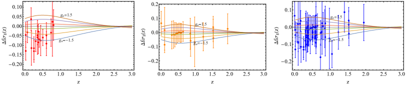
Figure 1: $\Delta f\sigma_{8}$ as a function of redshift for various values of $g_{\alpha}$ superimposed with the early growth data (left panel), late data (middle panel) and full growth data (right panel).

The evolution of the linear matter density growth factor $\delta\equiv\delta\rho/\rho$ in the context of both GR and most modified gravity theories on subhorizon scales is described by the equation

$${\ddot{\delta}}+2H{\dot{\delta}}-4\pi G_{\rm eff}\,\rho\,\delta\approx 0$$ (1)

where $\rho$ is the background matter density and $G_{\rm eff}$ is the effective Newton’s constant (which in general depends on redshift $z$ and cosmological scale $k$), and $H$ is the Hubble parameter. In terms of the redshift $z$, Eq. (1) takes the form

$$\delta^{\prime\prime}+\left(\frac{(H(z)^{2})^{\prime}}{2~{}H(z)^{2}}-{1\over 1+z}\right)\delta^{\prime}-{3\over 2}\frac{(1+z)~{}\Omega_{m}~{}G_{eff}(z,k)/G_{N}}{H(z)^{2}/H_{0}^{2}}~{}\delta=0$$ (2)

while in terms of the scale factor we have

$$\delta^{\prime\prime}(a)+\left(\frac{3}{a}+\frac{H^{\prime}(a)}{H(a)}\right)\delta^{\prime}(a)-\frac{3}{2}\frac{\Omega_{m}G_{eff}(a,k)/G_{N}}{a^{5}H(a)^{2}/H_{0}^{2}}\delta(a)=0$$ (3)

$G_{eff}$ arises from a generalized Poisson equation

$$\nabla^{2}\phi\approx 4\pi G_{\rm eff}\rho\;\delta$$ (4)

where $\phi$ is the perturbed metric potential in the Newtonian gauge where the perturbed FRW metric takes the form

$$ds^{2}=-(1+2\phi)dt^{2}+a^{2}(1-2\psi)d{\vec{x}}\,^{2}$$ (5)

GR predicts a constant homogeneous $G_{\rm eff}(z,k)=G_{N}$ ($G_{N}$ is Newton’s constant as measured by local experiments)

Constraints from Solar System Nesseris and Perivolaropoulos (2007) and nucleosynthesis tests Copi et al. (2004) imply that $G_{\rm eff}$ is close to the GR predicted form in both low and high redshifts. In particular at low $z$ we have Nesseris and Perivolaropoulos (2007)

$$\Big{\lvert}\frac{1}{G_{N}}\frac{dG_{\rm eff}(z)}{dz}|_{z=0}\Big{\rvert}<10^{-3}h^{-1}$$ (6)

while the second derivative is effectively unconstrained since

$$\Big{|}\frac{1}{G_{N}}\frac{d^{2}G_{\rm eff}(z)}{dz^{2}}|_{z=0}\Big{|}<10^{5}h^{-2}$$ (7)

At high $z$ Copi et al. (2004) and at $1\sigma$, we have

$$\lvert G_{\rm eff}/G_{N}-1\rvert\leq 0.2$$ (8)

A parametrization of $G_{\rm eff}(z)$ respecting these constraints is of the form Nesseris et al. (2017)

$$\frac{G_{\textrm{eff}}(a,g_{a},n)}{G_{\textrm{N}}} = 1+g_{a}(1-a)^{n}-g_{a}(1-a)^{n+m}$$ (9)

$$= 1+g_{a}\left(\frac{z}{1+z}\right)^{n}-g_{a}\left(\frac{z}{1+z}\right)^{n+m}.$$

where $n$ and $m$ are integer parameters with $n\geq 2$ and $m>0$. Here we set $n=m=2$.

The observable $f\sigma_{8}(a)$ can be obtained from the solution $\delta(a)$ of Eq. (3) using the definitions $f(a)\equiv d\ln\delta(a)/d\ln a$ and $\sigma(a)=\sigma_{8}\frac{\delta(a)}{\delta(1)}$. Thus, we have Percival (2005)

$${\rm{\it f\sigma}}_{8}(a) \equiv f(a)\cdot\sigma(a)$$ (10)

$$= \frac{\sigma_{8}}{\delta(1)}~{}a~{}\delta^{\prime}(a),$$ (11)

Therefore, both $f\sigma_{8}(a)$ and the growth rate $f(a)$ [or equivalently $f\sigma_{8}(z)$ and $f(z$)] can be obtained by numerically solving Eq. (2) or (3). The solution of these equations requires the specification of proper parametrizations for both the background expansion $H(z)$ and the effective Newton’s constant $G_{eff}(z)$. In the context of the present analysis we assume a flat universe and a $wCDM$ model background expansion of the form

$$H^{2}(z)=H_{0}^{2}\left[\Omega_{m}(1+z)^{3}+(1-\Omega_{m})(1+z)^{3(1+w)}\right]\Rightarrow$$

$$E^{2}(z)=\frac{H^{2}(z)}{H_{0}^{2}}=\Omega_{m}(1+z)^{3}+(1-\Omega_{m})(1+z)^{3(1+w)}$$ (12)

and $G_{eff}$ parametrized by Eq. (9) with $n=m=2$. Using these parametrizations and initial conditions corresponding to GR in the matter era [$\delta(a)\sim a$] it is straightforward to obtain the predicted evolution of the observables $f\sigma_{8}(z)$ and $f(z)$ for various parameter values around the standard Planck15/$\Lambda$CDM model parameters ($\Omega_{m}^{P}=0.31$, $w=-1$, $g_{a}=0$). For each observable $O(\Omega_{m},w,g_{a})$ [e.g. $f\sigma_{8}(z)$] we consider the deviation

$$\Delta O_{\Omega_{m}}\equiv O(\Omega_{m},-1,0)-O(\Omega_{m}^{P},-1,0)$$ (13)

Similar deviations $\Delta O_{w}$ and $\Delta O_{g_{a}}$ are defined for the other two parameters in the context of a given observable $O$.

In Fig. 1 we show the deviation $\Delta f\sigma_{8g_{a}}$ for $g_{a}$ in the range $g_{a}\in[-1.5,1.5]$ superposed with a recent compilation of the $f\sigma_{8}(z)$ data Kazantzidis and Perivolaropoulos (2018) shown in Table LABEL:tab:data-rsd in the Appendix (with early data published before 2015 in the left panel, recent data published after 2016 in the middle panel and full dataset in the right panel). No fiducial model correction has been implemented for the datapoints shown, but such a correction would lead to a change of no more than about $3\%$ Macaulay et al. (2013); Kazantzidis and Perivolaropoulos (2018). There are three interesting points to be noted in Fig. 1.

1. Early data favor weaker gravity ($g_{a}<0$) for redshifts around $z\simeq 0.5$ assuming a fixed Planck15/$\Lambda$CDM background. This trend is well known Macaulay et al. (2013) and has been demonstrated and discussed extensively, e.g. in Refs. Nesseris et al. (2017); Gomez-Valent and Sola (2017); Gómez-Valent and Solà (2018); Basilakos and Nesseris (2017, 2016); Alam et al. (2016); L’Huillier et al. (2017); Sagredo et al. (2018); Arjona et al. (2018).

2. The observable $f\sigma_{8}(z)$ has a blind spot with respect to the parameter $g_{a}$ at redshift $z\simeq 2.7$. Such a blind spot was also pointed out in Ref. Nesseris et al. (2011) with respect to a similar gravitational strength parameter (where it was called “sweet spot” in that Ref. Nesseris et al. (2011) even though the term “blind spot” should have been used).

3. There is a redshift range around $z\simeq 0.5$ of optimal sensitivity of the observable $f\sigma_{8}(z)$ with respect to the parameter $g_{a}$. Despite of the existence of this optimal redshift range much of the recent $f\sigma_{8}(z)$ data appear at larger redshifts approaching the blind spot region. These datapoints have reduced sensitivity in identifying deviations of $G_{eff}$ from its GR value $G_{N}$

The existence of blind spots and optimal redshifts of an observable $O$ with respect to a cosmological parameter $P$ may also be quantified by defining the “sensitivity” measure including the effects of the survey volume $V_{eff}(k,z)$. The effective survey volume probed for a particular k mode with the power spectrum $p(k,z)$ in a survey of sky area surveyed $\Delta\Omega$ is given by

$$V_{eff}(k,z)=\Delta\Omega\int_{0}^{z}\left[\frac{n(z^{\prime})p(k,z^{\prime})}{1+n(z^{\prime})p(k,z^{\prime})}\right]^{2}\frac{dV}{dz^{\prime}d\Omega}dz^{\prime}$$ (14)

where $z$ is the maximum redshift corresponding to the survey volume $V_{eff}$ and $n(z)$ is the number density of galaxies that are detected, which is given as

$$n(z)=\int_{M_{lim}(z)}^{\infty}\frac{dN}{dVdM}dM$$ (15)

The function $M_{lim}(z)$ is the limiting mass threshold which is detected for the given survey and $dV$ is the infinitesimal comoving volume element

$$dV=\frac{r^{2}(z)}{H(z)}d\Omega\,dz$$ (16)

where

$$r(z)=\frac{c}{H_{0}}\int_{0}^{z}\frac{dz^{\prime}}{E(z^{\prime})}$$ (17)

and $E(z^{\prime})$ is given by Eq. (12)

The constraining power of the observable $O$ depends on the survey volume $V_{eff}(k,z)$, since the error $\sigma_{p}$ on the measurement of the power spectrum $p(k,z)$ increases as the effective survey volume $V_{eff}(k,z)$ decreases (i.e. as less $k$ modes are measured by the survey) as Feldman et al. (1994); Huelga et al. (1997); Duffy (2014); Abdalla and Rawlings (2005)

$$\left(\frac{\sigma_{p}}{p(k,z)}\right)^{2}=\frac{2}{4\pi k^{3}\Delta(log\,k)}\frac{(2\pi)^{3}}{V_{eff}(k,z)}\left[\frac{1+n(z)p(k,z)}{n(z)p(k,z)}\right]^{2}$$ (18)

Thus, since the error $\sigma_{p}$ on the measurement of the power spectrum $p(k,z)$ is inversely proportional to the square root of he survey volume $V_{eff}(k,z)$ [see Eq. (18)], we define the “sensitivity” measure as

$$S_{P}^{O}\equiv\frac{\Delta O(P)}{\Delta P}\cdot V_{eff}(k,z)^{1/2}$$ (19)

where $\Delta O$ is the deviation of the observable $O$ when a given parameter varies in a fixed small range $\Delta P=P_{max}-P_{min}$ around a fiducial model value (e.g. Planck15/$\Lambda$CDM). In Fig. 2 we show a plot of the sensitivity measure $S$ for the observable $f\sigma_{8}(z)$ and the three parameters $\Omega_{m}$, $w$, $g_{a}$. The existence of blind spots is manifest as roots of the sensitivity measure, while optimal redshifts appear as maxima of the magnitude of $S$. We have fixed $k$ such as that $np=3$ assuming sufficient signal to noise per pixel Duffy (2014). We have also rescaled sensitivity measure statistic so that it is unity at its maximum absolute value. The nonlinear modes may be excluded by setting a minimum redshift which is of $O(10^{-2})$ and are much smaller than the derived optimal redshifts and blind spots identified in our analysis. Notice that the sensitivity measure indicates the presence of blind spots for all three parameters. For $w$ the blind spot is close to $z\simeq 2$ while for $\Omega_{m}$ is close to $z\simeq 1$. The corresponding optimal redshifts are at $z\simeq 1.2$ for $g_{a}$, at $z\simeq 0.8$ for $w$ and at $z\simeq 0.5$ for $\Omega_{m}$. (Although the region $z>2$ for $w$ and $\Omega_{m}$ provides better sensitivity, there are currently almost no data available in this redshift range). Notice also in Figs. 1 and 2 that when including the effects of the survey volume the optimal redshifts shift to somewhat higher redshifts, while the blind spots remain unaffected.

As shown in Figs. 3 and 4 for both cases, recent data approach the blind spot regions in contrast to early published data that efficiently probed the optimal redshift regions for both parameters $w$ and $\Omega_{m}$. Also, early data seem to favor weaker growth of perturbations which occurs for lower, $g_{a}$, and $\Omega_{m}$ and higher $w$ Macaulay et al. (2013); Nesseris et al. (2017); Kazantzidis and Perivolaropoulos (2018). If this trend is partly attributed to a lower value of $G_{eff}$ in the recent past, then it is difficult to reconcile with the most generic modified gravity theories like $f(R)$ and scalar tensor theories Nesseris et al. (2017); Gannouji et al. (2018)

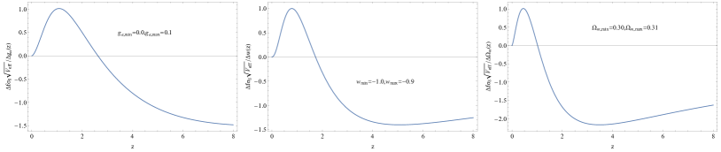
Figure 2: The sensitivity measure of $\frac{\Delta f\sigma_{8}}{\Delta P}V_{eff}^{1/2}$ for $P=g_{\alpha}$ (left panel), $P=w$ (middle panel), and $P=\Omega_{m}$ (right panel)

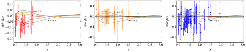
Figure 3: Same as Fig. 1 for various values of $w$.

Figure 4: Same as Fig. 1 for various values of $\Omega_{m}$.

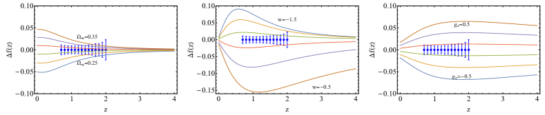
Figure 5: $\Delta f(z)$ as a function of redshift superimposed with the Euclid mock data for different values of $\Omega_{m}$ (left panel), $w$ (middle panel), and $g_{\alpha}$ (right panel).

A similar analysis can be performed for the growth rate observable $f(z)$ which will be probed by the Euclid mission Amendola et al. (2018). Mock Euclid data assuming a Planck15/$\Lambda$CDM fiducial model are shown in Fig. 5 with proper redshifts and error bars Amendola et al. (2018) along with the deviation of the observable $f(z)$ with respect to $\Omega_{m}$ (left panel), $w$ (middle panel) and $g_{a}$ (right panel). Clearly, the predicted redshift range of the Euclid data is optimal for the identification of new gravitational physics (right panel), but it is not optimized for constraining the matter density parameter (left panel of Fig. 5) or the equation of state parameter if $w<-1$ (middle panel).

The observable $f(z)$ is considered due to the approach of Ref. Amendola et al. (2018), where the Euclid team indicated that the large number of galaxies of the Euclid survey combined with the depth of the survey will allow a reliable estimate of the bias simultaneously with the growth rate $f(z)$ obtained through the redshift distortion $\beta$. The redshift distortion $\beta$ is defined as

$$\beta(z)=\frac{\Omega_{m}(z)^{\gamma}}{b(z)}=\frac{f(z)}{b(z)}$$ (20)

where $b(z)$ is the bias. Thus, the survey will not only probe the bias-free combination $f\sigma_{8}$, but also directly probe the growth observable $f(z)$ which is modeled in Ref. Amendola et al. (2018) with errorbars and is also considered separately in our analysis. Of course, what is actually observable is the redshift distortion $\beta$ parameter which is obtained through the ratio between the monopoles of the correlation functions in real and in redshift space. Thus, the derived blind spot and optimal redshift for the growth rate $f(z)$ are accurate under the assumption that the bias $b(z)$ has a very weak dependence on the redshift.

III Baryon Acoustic Oscillations: the Observables $D_{V}(z)\times\frac{r_{s}^{fid}}{r_{s}}$, $H\times\frac{r_{s}}{r_{s}^{fid}}$ and $D_{A}\times\frac{r_{s}^{fid}}{r_{s}}$

III.1 BAO Observables and their Variation with Cosmological Parameters.

Waves induced by radiation pressure in the pre-recombination plasma inflict a characteristic BAO scale on the late-time matter clustering at the radius of the sound horizon, defined as

$$r_{s}=\int_{z_{d}}^{\infty}\frac{c_{s}(z)}{H(z)}dz$$ (21)

where $c_{s}$ is given by Komatsu et al. (2009)

$$c_{s}(z)=\frac{c}{\sqrt{3\left(1+\frac{3\Omega_{b}}{4\Omega_{\gamma}}\frac{1}{1+z}\right)}}$$ (22)

and the drag redshift $z_{d}$ corresponds to times shortly after recombination, when photons decouple from baryons Aubourg et al. (2015). This BAO scale appears as a peak in the correlation function or equivalently as damped oscillations in the large scale structure power spectrum. In the context of standard matter and radiation epochs, the Planck 2015 measurements of the matter and baryon densities $\Omega_{m}$ and $\Omega_{b}$ specify the BAO scale to great accuracy (uncertainty less than $1\%$). An anisotropic BAO analysis measuring the sound horizon scale along the line of sight and along the transverse direction can measure both $H(z)$ and the comoving angular diameter distance $D_{M}(z)$ related to the physical angular diameter distance in a flat universe

$$D_{A}(z)=\frac{1}{1+z}\int_{0}^{z}\frac{c\;dz}{H(z)}$$ (23)

as $D_{M}(z)=(1+z)D_{A}(z)$ Bautista et al. (2017a). Deviation of cosmological parameters can change $r_{s}$, so BAO measurements actually constrain the combinations $D_{M}(z)\times\frac{r_{s}^{fid}}{r_{s}}$ or equivalently $D_{A}(z)\times\frac{r_{s}^{fid}}{r_{s}}$, $H(z)\times\frac{r_{s}}{r_{s}^{fid}}$ where $r_{s}^{fid}$ is the sound horizon (BAO scale) in the context of the fiducial cosmology assumed in the construction of the large-scale structure correlation function. An angle-averaged galaxy BAO measurement constrains the combination

$$D_{V}(z)=\left[czD_{M}(z)^{2}/H(z)\right]^{1/3}$$ (24)

Taking into account the variation of cosmological parameters the constrained combination becomes $D_{V}(z)\times\frac{r_{s}^{fid}}{r_{s}}$. Statistical isotropy can be used to constrain the observable combination $H(z)D_{M}(z)$ using an anisotropic BAO analysis in the context of the Alcock-Paczynski test Alcock and Paczynski (1979). The sound horizon $r_{s}(z_{d})$ at the drag epoch $z_{d}$ that enters the BAO observables may be calculated in the context of a given cosmological model, either numerically (e.g. with CAMB Lewis et al. (2000)) or using a fitting formula for $z_{d}$ Eisenstein and Hu (1998) of the form

$$z_{d}=\frac{1291(\Omega_{m}h^{2})^{0.251}}{1+0.659(\Omega_{m}h^{2})^{0.828}}\left[1+b_{1}(\Omega_{b}h^{2})^{b_{2}}\right]$$ (25)

where

$$b_{1} = 0.313(\Omega_{m}h^{2})^{-0.419}\left[1+0.607(\Omega_{m}h^{2})^{0.674}\right]$$ (26)

$$b_{2} = 0.238(\Omega_{m}h^{2})^{0.223}$$ (27)

and from Eq. (21)

$$r_{s}(z)=\frac{c}{\sqrt{3}}\int_{z_{d}}^{\infty}\frac{dz}{H(z)\sqrt{1+\frac{3\Omega_{b}}{4\Omega_{\gamma}}\frac{1}{1+z}}}$$ (28)

where $\Omega_{\gamma}=2.469\times 10^{-5}h^{-2}$ for $T_{\rm cmb}=2.725$ K, and

$$H(z)=H_{0}\left[\Omega_{m}(1+z)^{3}+\Omega_{r}(1+z)^{4}+\Omega_{\Lambda}(1+z)^{3(1+w)}\right]^{1/2}$$ (29)

with $\Omega_{r}=\Omega_{\gamma}(1+0.2271N_{eff})$ ($N_{eff}\simeq 3$ is the number of neutrino species) and

$$\Omega_{m}+\Omega_{r}+\Omega_{\Lambda}=1$$ (30)

in the context of a flat universe. It has been shown Hamann et al. (2010) that when the fitting formula is used to obtain $z_{d}$ close to the Planck15/$\Lambda$CDM parameter values, a correction factor of $154.66/150.82$ should be used on $r_{s}$ obtained from Eq. (28) to obtain agreement with the more accurate numerical estimate of $r_{s}$. Using Eqs. (23), (24), (28) and a Planck15/$\Lambda$CDM fiducial cosmology ($h=0.676$, $\Omega_{b}h^{2}=0.0223$, $\Omega_{m}=0.31$ and $r_{s}^{fid}=147.49$ Mpc), it is straightforward to construct the theoretically predicted redshift dependence of the BAO observables $D_{V}(z)\times\frac{r_{s}^{fid}}{r_{s}}$, $H\times\frac{r_{s}}{r_{s}^{fid}}$ and $D_{A}\times\frac{r_{s}^{fid}}{r_{s}}$ for various values of the parameters $\Omega_{m}$ and $w$ and superpose this dependence with corresponding currently available data shown in Table LABEL:tab:data-bao in the Appendix.

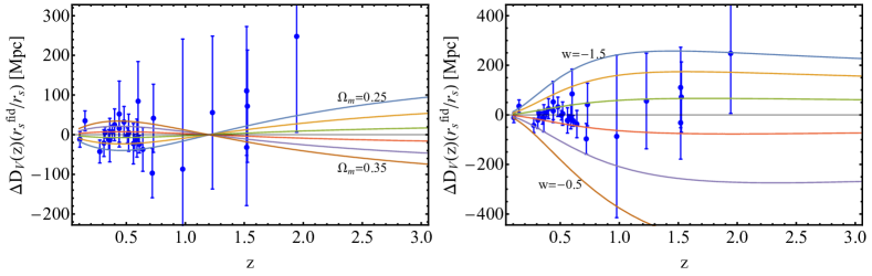
Figure 6: The deviation $\Delta$$D_{V}(z)\times\frac{r_{s}^{fid}}{r_{s}}$ as a function of the redshift $z$ for different values of $\Omega_{m}$ (left panel) and $w$ (right panel).

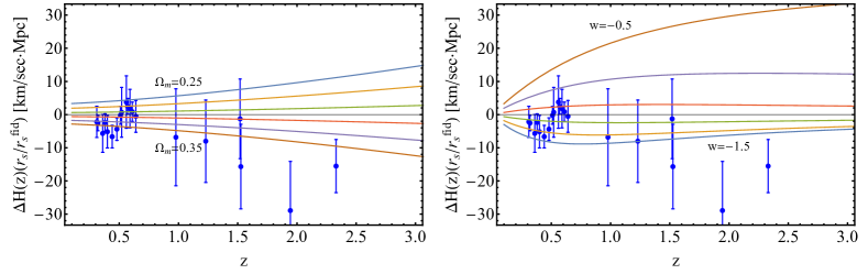
Figure 7: The deviation $\Delta$$H\times\frac{r_{s}}{r_{s}^{fid}}$ as a function of the redshift $z$ for different values of $\Omega_{m}$ (left panel) and $w$ (right panel)

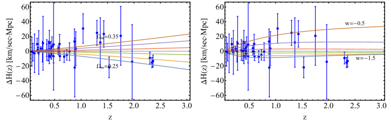
Figure 8: The deviation $\Delta H(z)$ as a function of redshift using the full compilation of Table LABEL:tab:data-hz in the Appendix, for various values of $\Omega_{m}$ (left panel) and $w$ (right panel).

In Fig. 6 we show the predicted evolution of the deviation of the observable $D_{V}(z)\times\frac{r_{s}^{fid}}{r_{s}}$ for various values of $\Omega_{m}$ (left panel) and of $w$ (right panel). The deviation of the parameter $\Omega_{m}$ (left panel) was performed around the value $\Omega_{m}=0.3$ while the deviation of the parameter $w$ was performed around the $\Lambda$CDM value $w=-1$ [see Eq. (13)]. Notice the existence of a blind spot at $z\simeq 1.2$ for the observable $D_{V}(z)\times\frac{r_{s}^{fid}}{r_{s}}$ with respect to the parameter $\Omega_{m}$, while the optimal redshift in the same plot is $z\simeq 0.6$. (Even though the region $z>2$ also seems to be optimal, there are currently almost no data available in this redshift range). In contrast, for the same observable with respect to the parameter $w$ there is no blind spot, while the optimal redshift range is at $z>1.2$.

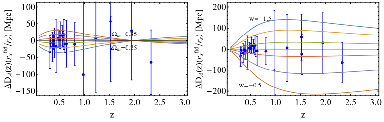
Figure 9: The deviation $\Delta$$D_{A}\times\frac{r_{s}^{fid}}{r_{s}}$ as a function of the redshift $z$ for different values of $\Omega_{m}$ (left panel) and $w$ (right panel)

In Fig. 7 we show the predicted evolution of the deviation of the observable $H\times\frac{r_{s}}{r_{s}^{fid}}$ for various values of $\Omega_{m}$ (left panel) and of $w$ (right panel). For this observable there is no blind redshift spot, while the sensitivity appears to increase monotonically with redshift for both observables. Notice the asymmetry obtained for the equation of state parameter which is due to the fact that for $w<-1$ at early times the effects of dark energy are negligible for all values of $w$, leading to a degeneracy for this range of parameters at high $z$. For comparison, in Fig. 8, we show the deviation of the observable Hubble expansion rate for various values of $\Omega_{m}$ (left panel) and of $w$ (right panel) along with corresponding data obtained from the spectroscopic evolution of galaxies used as cosmic chronometers, shown in Table LABEL:tab:data-hz in the Appendix along with the corresponding citations (for previous compilations see also Refs. Moresco et al. (2016); Anagnostopoulos and Basilakos (2018); Guo and Zhang (2016)). Even though Figs. 7 and 8 are qualitatively similar, it is clear that the BAO data are significantly more constraining compared to the cosmic chronometer data with respect to both parameters $\Omega_{m}$ and $w$, especially at low redshifts.

In Fig. 9 we show the predicted evolution of the deviation of the observable $D_{A}\times\frac{r_{s}^{fid}}{r_{s}}$ for various values of $\Omega_{m}$ (left panel) and $w$ (right panel). The behavior of this observable is similar to that of $D_{V}(z)\times\frac{r_{s}^{fid}}{r_{s}}$ even though the blind spot with respect to the parameter $\Omega_{m}$ appears at a higher redshift ($z\simeq 2$), while at higher redshifts the sensitivity of this observable with respect to the parameter $\Omega_{m}$ is significantly reduced compared to the sensitivity of $D_{V}(z)\times\frac{r_{s}^{fid}}{r_{s}}$.

A comparison of the three BAO observable distances $\frac{D_{M}(z)}{r_{s}\sqrt{z}}$, $\frac{D_{V}(z)}{r_{s}\sqrt{z}}$ and $\frac{zD_{H}(z)}{r_{s}\sqrt{z}}$ [as $D_{H}(z)=\frac{c}{H(z)}$] for the Planck15/$\Lambda$CDM best fit parameter values along with the corresponding data from Table LABEL:tab:data-bao of the Appendix is shown in Fig. 10.

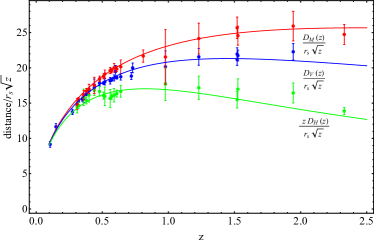
Figure 10: The BAO observable distances for the Planck15/$\Lambda$CDM best-fit parameter values along with the corresponding data from Table LABEL:tab:data-bao in the Appendix. The data appear to be in good agreement with the Planck15/$\Lambda$CDM predictions.

This plot is in excellent agreement with the corresponding plot of Ref. Alam et al. (2017) (Fig. 14) even though here we superpose the Planck15/$\Lambda$CDM prediction with a significantly larger compilation of datapoints. As demonstrated in the next subsection the BAO data are in good agreement with the Planck15/$\Lambda$CDM parameter values.

III.2 Contour Shapes and Redshift Ranges

The existence of optimal and blind redshift ranges for the BAO observables with respect to cosmological parameters has an effect on the form of maximum likelihood contours obtained from data at various redshift ranges. In particular, the Figure of Merit (reciprocal of the area of confidence contours in parameter space) tends to decrease for datasets with redshifts close to blind redshift spots and increase for datasets with redshifts close to optimal redshift regions. In order to demonstrate this effect, we construct the confidence contours for the parameters $\Omega_{m}$ and $w$ using the BAO observables in different redshift regions.

In order to construct $\chi^{2}$ we first consider the vector

$$V^{i}_{BAO}(z_{i},\Omega_{m},w)\equiv BAO^{m}_{i}-BAO^{m}_{theoretical}$$ (31)

Figure 11: The $1\sigma-3\sigma$ contours in the $\Omega_{m}-w$ parametric space. The contours describe the corresponding confidence regions using the full compilation of $D_{V}(z)\times\frac{r_{s}^{fid}}{r_{s}}$ data (left panel), low redshift ($z<0.55$) data (middle panel) and high redshift ($z>0.55$) data (right panel) from Table LABEL:tab:data-bao in the Appendix. The red and green dots describe the Planck15/$\Lambda$CDM best fit and the best-fit values from the compilation of $D_{V}(z)\times\frac{r_{s}^{fid}}{r_{s}}$ data. Notice that at high $z$ close to the blind spot for $\Omega_{m}$ and the optimum redshift for $w$, the thickness of the contours (uncertainty) increases along the $\Omega_{m}$ axis and decreases along the $w$ axis (the contours are rotated clockwise) as expected from Fig. 6.

where $m$ runs from 1 to 3 indicating the different types of BAO data of Table LABEL:tab:data-bao in the Appendix and the theoretical expressions for $D_{A}\times\frac{r_{s}^{fid}}{r_{s}}$, $D_{V}(z)\times\frac{r_{s}^{fid}}{r_{s}}$ and $H\times\frac{r_{s}}{r_{s}^{fid}}$ are given in Eqs. (23), (24) and (29) respectively. $\chi^{2}$ is obtained as

$$\chi^{2}=V^{i}F_{ij}V^{j}$$ (32)

where $F_{ij}$ is the Fisher matrix (inverse of the covariance matrix $C_{ij}$).

The covariance matrix for the $D_{V}(z)\times\frac{r_{s}^{fid}}{r_{s}}$ data takes the form

$$C_{ij,D_{V}\times\left(r_{s}^{fid.}/r_{s}\right)}^{\textrm{BAO,total}}=\left(\begin{array}[]{cccc}\sigma_{1}^{2}&0&0&\cdots\\ 0&C_{ij}^{WiggleZ}&0&\cdots\\ 0&0&\cdots&\sigma_{N}^{2}\\ \end{array}\right)$$ (33)

where $N=28$ and Kazin et al. (2014)

$$C_{ij}^{WiggleZ}=F_{ij,\text{WiggleZ}}^{-1}=10^{4}\left(\begin{array}[]{ccc}2.18&-1.12&0.47\\ -1.12&1.71&-0.72\\ 0.47&-0.72&1.65\\ \end{array}\right)^{-1}$$ (34)

whereas for both $D_{A}\times\frac{r_{s}^{fid}}{r_{s}}$ and $H\times\frac{r_{s}}{r_{s}^{fid}}$ we have assumed a diagonal covariance matrix

$$C_{ij}^{\textrm{BAO,total}}=\left(\begin{array}[]{cccc}\sigma_{1}^{2}&0&0&\cdots\\ 0&\sigma_{2}^{2}&0&\cdots\\ 0&0&\cdots&\sigma_{N}^{2}\\ \end{array}\right)$$ (35)

where $N$ is equal to the considered number of datapoints.

The forms of Eqs. (33) and (35) are clearly oversimplifications of the actual covariance matrices, since these forms ignore possible correlations between the considered BAO data. However, to the best of our knowledge the non-diagonal terms of the $D_{A}$ and $H$ covariance matrices are not publicly available. In order to estimate the magnitude of the effects of these terms we have performed Monte Carlo simulations including random nondiagonal terms to the covariance matrices for $D_{A}$ and $H$ of relative magnitude similar to the nondiagonal terms of the nondiagonal terms corresponding to $D_{V}$ setting the magnitude of the matrix Kazantzidis and Perivolaropoulos (2018)

$$C_{ij}=\frac{1}{2}\sigma_{i}\cdot\sigma_{j}$$ (36)

where $\sigma_{i}$ and $\sigma_{j}$ are the errors of the published datapoints $i$ and $j$ respectively. These simulations indicated that the likelihood contours and the best fit parameter values do not change more than $10\%$ when we include the nondiagonal terms in the covariance matrix. Thus, possible reasonable correlations among datapoints are not expected to significantly affect our results sup .

In the left panel of Fig. 11 we show the $1\sigma-3\sigma$ $\Omega_{m}-w$ contour plots for the full $D_{V}(z)\times\frac{r_{s}^{fid}}{r_{s}}$ data of Table LABEL:tab:data-bao in the Appendix using Eqs. (31)-(33) and ignoring the possible correlations among the datapoints. The best fit parameter values are within $1\sigma$ from the corresponding best fit Planck15/$\Lambda$CDM values (red dot).

Furthermore we construct the same contour plots for low-redshift $D_{V}(z)\times\frac{r_{s}^{fid}}{r_{s}}$ data (middle panel of Fig. 11), where $z<0.55$ (14 datapoints), and for high-redshift $D_{V}(z)\times\frac{r_{s}^{fid}}{r_{s}}$ data (right panel of Fig. 11), where $z>0.55$ (14 datapoints). The low-redshift data correspond to optimal redshift for the parameter $\Omega_{m}$ (see Fig. 6) and thus the confidence contours are thinner in the direction of the $\Omega_{m}$ axis while the contours are elongated in the $w$ direction. In contrast the high-redshift data are close to the $\Omega_{m}$ blind spot and thus the confidence contours are thicker in the $\Omega_{m}$ direction (left panel), while the contours are suppressed in the $w$ direction (as expected from Fig. 6) which indicates an optimal high-redshift range for the parameter $w$.

Similar conclusions and confidence contours are obtained from the low and high redshift data for $D_{A}\times\frac{r_{s}^{fid}}{r_{s}}$ and $H\times\frac{r_{s}}{r_{s}^{fid}}$ data (see Supplemental Material sup ).

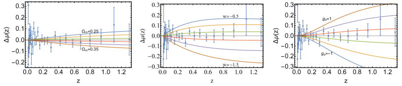
Figure 12: The deviation of the distance modulus observable $\Delta\mu$ as a function of redshift for $\Omega_{m}$ (left panel), $w$ (middle panel) and $g_{\alpha}$ (right panel) superimposed with the JLA data of Table LABEL:tab:data-jla in the Appendix.

Figure 13: The sensitivity measure as a function of redshift $z$ for $\Omega_{m}$ (left panel), $g_{\alpha}$ (middle panel) and $w$ (right panel).

IV Distance Moduli from SnIa and from Gravitational Waves

The luminosity distance

$$D_{L}(z;\Omega_{m},w)=(1+z)\int_{0}^{z}\frac{c\;dz}{H(z;\Omega_{m},w)}$$ (37)

is an important cosmological observable that is measured using standard candles like SnIa or standard gravitational wave sirens, like merging binary neutron star systems observed via multi-messenger observations. The distance modulus $\mu=m-M$ is the difference between the apparent magnitude $m$ and the absolute magnitude M of standard candle. It is related to the luminosity distance $D_{L}$ in Mpc as

$$\mu(z;\Omega_{m},w)=5log_{10}(D_{L})+25$$ (38)

In the context of a varying effective Newton’s constant $G_{eff}(z)$ the absolute magnitude of SnIa is expected to vary with redshift as Garcia-Berro et al. (1999); Gaztanaga et al. (2002); Nesseris and Perivolaropoulos (2006)

$$M-M_{0}=\frac{15}{4}log_{10}\left(\frac{G_{eff}}{G_{N}}\right)$$ (39)

where the subscript $0$ refers to local value of $M$. Thus, for SnIa $\mu$ also depends on the evolution of $G_{eff}(z)$ (or equivalently on the parameter $g_{a}$) as

$$\mu(z;\Omega_{m},w,g_{a})=5log_{10}(D_{L})+\frac{15}{4}log_{10}\left(\frac{G_{eff}(z;g_{a})}{G_{N}}\right)+25$$ (40)

In the case of gravitational wave luminosity distance, the corresponding gravitational wave distance modulus obtained from standard sirens is of the form Belgacem et al. (2018)

$$\mu_{gw}(z;\Omega_{m},w,g_{a})=5log_{10}\left(D_{L}\sqrt{\frac{G_{eff}}{G_{N}}}\right)+25$$ (41)

In Fig. 12 we show the deviation $\Delta\mu$ as a function of redshift for $\Omega_{m}$ (left panel), $w$ (middle panel) and $g_{\alpha}$ (right panel) superimposed with the JLA SnIa binned data of Table LABEL:tab:data-jla in the Appendix. The corresponding sensitivity measure is shown in Fig. 13. Notice that even though the deviation $\Delta\mu_{gw}$ appears to be increasing with redshift for all the parameters considered, the absolute value of the sensitivity measure with respect to the parameter $g_{a}$ has a maximum for redshifts in the range $z\in[4,5]$, indicating the presence of an optimal redshift range.

The deviations $\Delta\mu_{gw}(z)$ with respect to the parameters $\Omega_{m}$ and $w$ is identical to the corresponding deviations $\Delta\mu(z)$, since for $g_{a}=0$ we have $\Delta\mu(z)=\Delta\mu_{gw}(z)$. The deviation $\Delta\mu_{gw}(z)$ with respect to the parameter $g_{a}$ is shown in Fig. 14

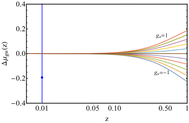
Figure 14: The deviation of the gravitational wave distance modulus with the parameter $g_{a}$. The only existing datapoint does not lead to any useful constraints.

along with the single available datapoint from the standard siren GW170817 Abbott (2017); Abbott et al. (2017a). Clearly even though standard siren data can in principle be used to constrain the evolution of $G_{eff}$, a dramatic improvement is required before such probes become competitive with growth and SnIa data.

V Discussion-Outlook

We have demonstrated that the constraining power (sensitivity) of a wide range of cosmological observables on cosmological parameters is a rapidly varying function of the redshift where the observable is measured. In fact, this sensitivity in many cases does not vary monotonically with redshift but has degeneracy points (redshift blind spots) and maxima (optimal redshift ranges) which are relatively close in redshift space. The identification of such regions can contribute to the optimal design and redshift range selection of cosmological probes aimed at constraining specific cosmological parameters through measurement of cosmological observables. In addition, we have shown that many of the recent $f\sigma_{8}(z)$ RSD data, which tend to be at higher redshifts ($z>0.8$) are close to blind spots of the observable $f\sigma_{8}(z)$ with respect to all three cosmological parameters considered ($\Omega_{m}$, $w$ and $g_{a}$). A similar trend for probing higher redshifts also exists for upcoming surveys as demonstrated in Table 1. A more efficient strategy for this observable would be an improvement of the measurements at lower redshifts instead of focusing on higher redshifts. Such a strategy would lead to improved constraints on all three parameters considered.

Even though our analysis has revealed the generic existence of optimal redshifts and blind spots of observables with respect to specific cosmological parameters, it still has not taken into account all relevant effects that play a role in determining the exact location of these points in redshift space. For example, we have not explicitly taken into account the number of linear modes available to a survey in redshift space as well as the dependence of the effective volume $V_{eff}$ on the number of tracers and their selection. We anticipate that these effects could mildly shift the location of the derived blind spots and optimal redshifts determined by our analysis.

An interesting extension of our analysis could involve the consideration of other observables and additional cosmological parameters (e.g. an equation of state parameter that evolves with redshift). The existence of blind spots could be avoided by considering various functions and/or combinations of cosmic observables designed in such a way as to optimize sensitivity for given cosmological parameters in a given redshift range. The investigation of the efficiency of such combinations is also an interesting extension of this project.

Appendix A Data Used in the Analysis

In this appendix we present the data used in the analysis.

Table 2: The compilation of RSD data used in the present analysis and in the analysis of Ref. Kazantzidis and Perivolaropoulos (2018)

Index	Dataset	$z$	$f\sigma_{8}(z)$	Refs.	Year	Fiducial Cosmology
1	SDSS-LRG	$0.35$	$0.440\pm 0.050$	Song and Percival (2009)	30 October 2006	$(\Omega_{m},\Omega_{K},\sigma_{8}$)$=(0.25,0,0.756)$Tegmark et al. (2006)
2	VVDS	$0.77$	$0.490\pm 0.18$	Song and Percival (2009)	6 October 2009	$(\Omega_{m},\Omega_{K},\sigma_{8})=(0.25,0,0.78)$
3	2dFGRS	$0.17$	$0.510\pm 0.060$	Song and Percival (2009)	6 October 2009	$(\Omega_{m},\Omega_{K})=(0.3,0,0.9)$
4	2MRS	0.02	$0.314\pm 0.048$	Davis et al. (2011), Hudson and Turnbull (2012)	13 Novemver 2010	$(\Omega_{m},\Omega_{K},\sigma_{8})=(0.266,0,0.65)$
5	SnIa+IRAS	0.02	$0.398\pm 0.065$	Turnbull et al. (2012), Hudson and Turnbull (2012)	20 October 2011	$(\Omega_{m},\Omega_{K},\sigma_{8})=(0.3,0,0.814)$
6	SDSS-LRG-200	$0.25$	$0.3512\pm 0.0583$	Samushia et al. (2012)	9 December 2011	$(\Omega_{m},\Omega_{K},\sigma_{8})=(0.276,0,0.8)$
7	SDSS-LRG-200	$0.37$	$0.4602\pm 0.0378$	Samushia et al. (2012)	9 December 2011
8	SDSS-LRG-60	$0.25$	$0.3665\pm 0.0601$	Samushia et al. (2012)	9 December 2011	$(\Omega_{m},\Omega_{K},\sigma_{8})=(0.276,0,0.8)$
9	SDSS-LRG-60	$0.37$	$0.4031\pm 0.0586$	Samushia et al. (2012)	9 December 2011
10	WiggleZ	$0.44$	$0.413\pm 0.080$	Blake et al. (2012)	12 June 2012	$(\Omega_{m},h,\sigma_{8})=(0.27,0.71,0.8)$
11	WiggleZ	$0.60$	$0.390\pm 0.063$	Blake et al. (2012)	12 June 2012
12	WiggleZ	$0.73$	$0.437\pm 0.072$	Blake et al. (2012)	12 June 2012
13	6dFGS	$0.067$	$0.423\pm 0.055$	Beutler et al. (2012)	4 July 2012	$(\Omega_{m},\Omega_{K},\sigma_{8})=(0.27,0,0.76)$
14	SDSS-BOSS	$0.30$	$0.407\pm 0.055$	Tojeiro et al. (2012)	11 August 2012	$(\Omega_{m},\Omega_{K},\sigma_{8})=(0.25,0,0.804)$
15	SDSS-BOSS	$0.40$	$0.419\pm 0.041$	Tojeiro et al. (2012)	11 August 2012
16	SDSS-BOSS	$0.50$	$0.427\pm 0.043$	Tojeiro et al. (2012)	11 August 2012
17	SDSS-BOSS	$0.60$	$0.433\pm 0.067$	Tojeiro et al. (2012)	11 August 2012
18	Vipers	$0.80$	$0.470\pm 0.080$	de la Torre et al. (2013)	9 July 2013	$(\Omega_{m},\Omega_{K},\sigma_{8})=(0.25,0,0.82)$
19	SDSS-DR7-LRG	$0.35$	$0.429\pm 0.089$	Chuang and Wang (2013)	8 August 2013	$(\Omega_{m},\Omega_{K},\sigma_{8}$)$=(0.25,0,0.809)$Komatsu et al. (2011)
20	GAMA	$0.18$	$0.360\pm 0.090$	Blake et al. (2013)	22 September 2013	$(\Omega_{m},\Omega_{K},\sigma_{8})=(0.27,0,0.8)$
21	GAMA	$0.38$	$0.440\pm 0.060$	Blake et al. (2013)	22 September 2013
22	BOSS-LOWZ	$0.32$	$0.384\pm 0.095$	Sanchez et al. (2014)	17 December 2013	$(\Omega_{m},\Omega_{K},\sigma_{8})=(0.274,0,0.8)$
23	SDSS DR10 and DR11	$0.32$	$0.48\pm 0.10$	Sanchez et al. (2014)	17 December 2013	$(\Omega_{m},\Omega_{K},\sigma_{8}$)$=(0.274,0,0.8)$Anderson et al. (2014b)
24	SDSS DR10 and DR11	$0.57$	$0.417\pm 0.045$	Sanchez et al. (2014)	17 December 2013
25	SDSS-MGS	$0.15$	$0.490\pm 0.145$	Howlett et al. (2015)	30 January 2015	$(\Omega_{m},h,\sigma_{8})=(0.31,0.67,0.83)$
26	SDSS-veloc	$0.10$	$0.370\pm 0.130$	Feix et al. (2015)	16 June 2015	$(\Omega_{m},\Omega_{K},\sigma_{8}$)$=(0.3,0,0.89)$Tegmark et al. (2004)
27	FastSound	$1.40$	$0.482\pm 0.116$	Okumura et al. (2016)	25 November 2015	$(\Omega_{m},\Omega_{K},\sigma_{8}$)$=(0.27,0,0.82)$Hinshaw et al. (2013b)
28	SDSS-CMASS	$0.59$	$0.488\pm 0.060$	Chuang et al. (2016)	8 July 2016	$\ \ (\Omega_{m},h,\sigma_{8})=(0.307115,0.6777,0.8288)$
29	BOSS DR12	$0.38$	$0.497\pm 0.045$	Alam et al. (2017)	11 July 2016	$(\Omega_{m},\Omega_{K},\sigma_{8})=(0.31,0,0.8)$
30	BOSS DR12	$0.51$	$0.458\pm 0.038$	Alam et al. (2017)	11 July 2016
31	BOSS DR12	$0.61$	$0.436\pm 0.034$	Alam et al. (2017)	11 July 2016
32	BOSS DR12	$0.38$	$0.477\pm 0.051$	Beutler et al. (2017)	11 July 2016	$(\Omega_{m},h,\sigma_{8})=(0.31,0.676,0.8)$
33	BOSS DR12	$0.51$	$0.453\pm 0.050$	Beutler et al. (2017)	11 July 2016
34	BOSS DR12	$0.61$	$0.410\pm 0.044$	Beutler et al. (2017)	11 July 2016
35	Vipers v7	$0.76$	$0.440\pm 0.040$	Wilson (2016)	26 October 2016	$(\Omega_{m},\sigma_{8})=(0.308,0.8149)$
36	Vipers v7	$1.05$	$0.280\pm 0.080$	Wilson (2016)	26 October 2016
37	BOSS LOWZ	$0.32$	$0.427\pm 0.056$	Gil-Marín et al. (2017)	26 October 2016	$(\Omega_{m},\Omega_{K},\sigma_{8})=(0.31,0,0.8475)$
38	BOSS CMASS	$0.57$	$0.426\pm 0.029$	Gil-Marín et al. (2017)	26 October 2016
39	Vipers	$0.727$	$0.296\pm 0.0765$	Hawken et al. (2017)	21 November 2016	$(\Omega_{m},\Omega_{K},\sigma_{8})=(0.31,0,0.7)$
40	6dFGS+SnIa	$0.02$	$0.428\pm 0.0465$	Huterer et al. (2017)	29 November 2016	$(\Omega_{m},h,\sigma_{8})=(0.3,0.683,0.8)$
41	Vipers	$0.6$	$0.48\pm 0.12$	de la Torre et al. (2017)	16 December 2016	$(\Omega_{m},\Omega_{b},n_{s},\sigma_{8}$)= $(0.3,0.045,0.96,0.831)$Ade et al. (2016)
42	Vipers	$0.86$	$0.48\pm 0.10$	de la Torre et al. (2017)	16 December 2016
43	Vipers PDR-2	$0.60$	$0.550\pm 0.120$	Pezzotta et al. (2017)	16 December 2016	$(\Omega_{m},\Omega_{b},\sigma_{8})=(0.3,0.045,0.823)$
44	Vipers PDR-2	$0.86$	$0.400\pm 0.110$	Pezzotta et al. (2017)	16 December 2016
45	SDSS DR13	$0.1$	$0.48\pm 0.16$	Feix et al. (2017)	22 December 2016	$(\Omega_{m},\sigma_{8}$)$=(0.25,0.89)$Tegmark et al. (2004)
46	2MTF	0.001	$0.505\pm 0.085$	Howlett et al. (2017)	16 June 2017	$(\Omega_{m},\sigma_{8})=(0.3121,0.815)$
47	Vipers PDR-2	$0.85$	$0.45\pm 0.11$	Mohammad et al. (2017)	31 July 2017	$(\Omega_{b},\Omega_{m},h)=(0.045,0.30,0.8)$
48	BOSS DR12	$0.31$	$0.469\pm 0.098$	Wang et al. (2017)	15 September 2017	$(\Omega_{m},h,\sigma_{8})=(0.307,0.6777,0.8288)$
49	BOSS DR12	$0.36$	$0.474\pm 0.097$	Wang et al. (2017)	15 September 2017
50	BOSS DR12	$0.40$	$0.473\pm 0.086$	Wang et al. (2017)	15 September 2017
51	BOSS DR12	$0.44$	$0.481\pm 0.076$	Wang et al. (2017)	15 September 2017
52	BOSS DR12	$0.48$	$0.482\pm 0.067$	Wang et al. (2017)	15 September 2017
53	BOSS DR12	$0.52$	$0.488\pm 0.065$	Wang et al. (2017)	15 September 2017
54	BOSS DR12	$0.56$	$0.482\pm 0.067$	Wang et al. (2017)	15 September 2017
55	BOSS DR12	$0.59$	$0.481\pm 0.066$	Wang et al. (2017)	15 September 2017
56	BOSS DR12	$0.64$	$0.486\pm 0.070$	Wang et al. (2017)	15 September 2017
57	SDSS DR7	$0.1$	$0.376\pm 0.038$	Shi et al. (2017)	12 December 2017	$(\Omega_{m},\Omega_{b},\sigma_{8})=(0.282,0.046,0.817)$
58	SDSS-IV	$1.52$	$0.420\pm 0.076$	Gil-Marín et al. (2018)	8 January 2018	$(\Omega_{m},\Omega_{b}h^{2},\sigma_{8})=(0.26479,0.02258,0.8)$
59	SDSS-IV	$1.52$	$0.396\pm 0.079$	Hou et al. (2018)	8 January 2018	$(\Omega_{m},\Omega_{b}h^{2},\sigma_{8})=(0.31,0.022,0.8225)$
60	SDSS-IV	$0.978$	$0.379\pm 0.176$	Zhao et al. (2018)	9 January 2018	$(\Omega_{m},\sigma_{8})=(0.31,0.8)$
61	SDSS-IV	$1.23$	$0.385\pm 0.099$	Zhao et al. (2018)	9 January 2018
62	SDSS-IV	$1.526$	$0.342\pm 0.070$	Zhao et al. (2018)	9 January 2018
63	SDSS-IV	$1.944$	$0.364\pm 0.106$	Zhao et al. (2018)	9 January 2018

Table 3: A compilation of BAO data that have been published from 2006 until 2018 in chronological order

Index	$z_{eff}$	$D_{A}\times\left(r_{s}^{fid.}/r_{s}\right)$ (Mpc)	$H(z)\times\left(r_{s}/r_{s}^{fid.}\right)$ (km/sec Mpc)	$D_{V}\times\left(r_{s}^{fid.}/r_{s}\right)$ (Mpc)	Year	Ref.
1	$0.275$	-	-	$1061.87\pm 29$	2 November 2009	Percival et al. (2010)
2	$0.106$	-	-	$439.3\pm 19.6$	16 June 2011	Beutler et al. (2011)
3	$0.35$	-	-	$1356\pm 25$	28 March 2012	Mehta et al. (2012)
4	$0.44$	-	-	$1716\pm 83$	28 July 2014	Kazin et al. (2014)
5	$0.60$	-	-	$2221\pm 100$	28 July 2014	Kazin et al. (2014)
6	$0.73$	-	-	$2516\pm 86$	28 July 2014	Kazin et al. (2014)
7	$0.15$	-	-	$664\pm 25$	21 January 2015	Ross et al. (2015)
8	$0.38$	$1100\pm 22$	$81.5\pm 2.6$	$1477\pm 16$	11 July 2016	Alam et al. (2017)
9	$0.51$	$1309.3\pm 24.5$	$90.5\pm 2.7$	$1877\pm 19$	11 July 2016	Alam et al. (2017)
10	$0.61$	$1418\pm 27.3$	$97.3\pm 2.9$	$2140\pm 22$	11 July 2016	Alam et al. (2017)
11	$0.32$	$980.3\pm 15.9$	$78.4\pm 2.3$	$1270\pm 14$	11 July 2016	Alam et al. (2017)
12	$0.57$	$1387.9\pm 22.3$	$96.6\pm 2.4$	$2033\pm 21$	11 July 2016	Alam et al. (2017)
13	$0.31$	$931.42\pm 48$	$78.3\pm 4.7$	$1208.36\pm 33.81$	6 December 2016	Zhao et al. (2017)
14	$0.36$	$1047.04\pm 44$	$77.2\pm 5.7$	$1388.36\pm 55$	6 December 2016	Zhao et al. (2017)
15	$0.40$	$1131.34\pm 44$	$79.72\pm 4.9$	$1560.06\pm 40$	6 December 2016	Zhao et al. (2017)
16	$0.44$	$1188.78\pm 32$	$80.29\pm 3.4$	$1679.88\pm 35$	6 December 2016	Zhao et al. (2017)
17	$0.48$	$1271.43\pm 25.8$	$84.69\pm 3.4$	$1820.44\pm 39$	6 December 2016	Zhao et al. (2017)
18	$0.52$	$1336.53\pm 39$	$91.97\pm 7.5$	$1913.54\pm 47$	6 December 2016	Zhao et al. (2017)
19	$0.56$	$1385.47\pm 30.5$	$97.3\pm 7.9$	$2001.91\pm 51$	6 December 2016	Zhao et al. (2017)
20	$0.59$	$1423.43\pm 44$	$97.07\pm 5.8$	$2100.43\pm 48$	6 December 2016	Zhao et al. (2017)
21	$0.64$	$1448.81\pm 69$	$97.70\pm 4.8$	$2207.51\pm 55$	6 December 2016	Zhao et al. (2017)
22	$2.33$	$1669.7\pm 96.1$	$224\pm 8$	-	27 March 2017	Bautista et al. (2017a)
23	$1.52$	-	-	$3843\pm 147$	16 October 2017	Ata et al. (2018)
24	$0.81$	$1586.7\pm 63.5$	-	-	17 December 2017	Abbott et al. (2017b)
25	$0.72$	-	-	$2353\pm 63$	21 December 2017	Bautista et al. (2017b)
26	$1.52$	$1850\pm 110$	$162\pm 12$	$3985.2\pm 162.4$	8 January 2018	Gil-Marín et al. (2018)
27	$0.978$	$1586.18\pm 284.93$	$113.72\pm 14.63$	$2933.59\pm 327.71$	16 January 2018	Zhao et al. (2018)
28	$1.230$	$1769.08\pm 159.67$	$131.44\pm 12.42$	$3522.04\pm 192.74$	16 January 2018	Zhao et al. (2018)
29	$1.526$	$1768.77\pm 96.59$	$148.11\pm 12.75$	$3954.31\pm 141.71$	16 January 2018	Zhao et al. (2018)
30	$1.944$	$1807.98\pm 146.46$	$172.63\pm 14.79$	$4575.17\pm 241.61$	16 January 2018	Zhao et al. (2018)

Table 4: The $H(z)$ data compilation presented in Ref. Jesus et al. (2018) and used in the present analysis.

Index	$z$	$H(z)$ (km/sec Mpc)	$\sigma_{H}$	Reference
1	$0.070$	$69$	$19.6$	Zhang et al. (2014)
2	$0.090$	$69$	$12$	Simon et al. (2005)
3	$0.120$	$68.6$	$26.2$	Zhang et al. (2014)
4	$0.170$	$83$	$8$	Simon et al. (2005)
5	$0.179$	$75$	$4$	Moresco et al. (2012)
6	$0.199$	$75$	$5$	Moresco et al. (2012)
7	0.200	72.9	29.6	Zhang et al. (2014)
8	0.240	79.69	6.65	Gaztanaga et al. (2009)
9	0.270	77	14	Simon et al. (2005)
10	0.280	88.8	36.6	Zhang et al. (2014)
11	0.300	81.7	6.22	Oka et al. (2014)
12	0.350	82.7	8.4	Chuang and Wang (2013)
13	0.352	83	14	Moresco et al. (2012)
14	0.3802	83	13.5	Moresco et al. (2016)
15	0.400	95	17	Simon et al. (2005)
16	0.4004	77	10.02	Moresco et al. (2016)
17	0.4247	87.1	11.2	Moresco et al. (2016)
18	0.430	86.45	3.68	Gaztanaga et al. (2009)
19	0.440	82.6	7.8	Blake et al. (2012)
20	0.4497	92.8	12.9	Moresco et al. (2016)
21	0.4783	80.9	9	Moresco et al. (2016)
22	0.480	97	62	Stern et al. (2010)
23	0.570	92.900	7.855	Anderson et al. (2014c)
24	0.593	104	13	Moresco et al. (2012)
25	0.6	87.9	6.1	Blake et al. (2012)
26	0.68	92	8	Moresco et al. (2012)
27	0.73	97.3	7.0	Blake et al. (2012)
28	0.781	105	12	Moresco et al. (2012)
29	0.875	125	17	Moresco et al. (2012)
30	0.88	90	40	Stern et al. (2010)
31	0.9	117	23	Simon et al. (2005)
32	1.037	154	20	Moresco et al. (2012)
33	1.300	168	17	Simon et al. (2005)
34	1.363	160	22.6	Moresco (2015)
35	1.43	177	18	Simon et al. (2005)
36	1.53	140	14	Simon et al. (2005)
37	1.75	202	40	Simon et al. (2005)
38	1.965	186.5	50.4	Moresco (2015)
39	2.300	224	8	Busca et al. (2013)
40	2.34	222	7	Delubac et al. (2015)
41	2.36	226	8	Font-Ribera et al. (2014)

Table 5: The JLA binned data used in the analysis from Ref. Betoule et al. (2014)

Index	$z$	$\mu$	$\sigma_{\mu}$
1	$0.01$	$32.9539$	$0.145886$
2	$0.012$	$33.879$	$0.167796$
3	$0.014$	$33.8421$	$0.0784989$
4	$0.016$	$34.1186$	$0.0723539$
5	$0.019$	$34.5934$	$0.0854606$
6	$0.023$	$34.939$	$0.0561251$
7	$0.026$	$35.2521$	$0.0610683$
8	$0.031$	$35.7485$	$0.0567639$
9	$0.037$	$36.0698$	$0.0567956$
10	$0.043$	$36.4346$	$0.0751431$
11	$0.051$	$36.6511$	$0.0929013$
12	$0.06$	$37.158$	$0.0620892$
13	$0.07$	$37.4302$	$0.0658793$
14	$0.082$	$37.9566$	$0.0546505$
15	$0.097$	$38.2533$	$0.0599337$
16	$0.114$	$38.6129$	$0.0374341$
17	$0.134$	$39.0679$	$0.0386141$
18	$0.158$	$39.3414$	$0.0346886$
19	$0.186$	$39.7921$	$0.0321403$
20	$0.218$	$40.1565$	$0.0329616$
21	$0.257$	$40.565$	$0.0317198$
22	$0.302$	$40.9053$	$0.0392622$
23	$0.355$	$41.4214$	$0.0335758$
24	$0.418$	$41.7909$	$0.0415207$
25	$0.491$	$42.2315$	$0.0393713$
26	$0.578$	$42.617$	$0.0359453$
27	$0.679$	$43.0527$	$0.0627778$
28	$0.799$	$43.5042$	$0.0545914$
29	$0.94$	$43.9726$	$0.0668276$
30	$1.105$	$44.5141$	$0.154604$
31	$1.3$	$44.8219$	$0.138452$

References

- Carroll (2001) Sean M. Carroll, “The Cosmological constant,” Living Rev. Rel. 4, 1 (2001), arXiv:astro-ph/0004075 [astro-ph] .
- Adam et al. (2016) R. Adam et al. (Planck), “Planck 2015 results. I. Overview of products and scientific results,” Astron. Astrophys. 594, A1 (2016), arXiv:1502.01582 [astro-ph.CO] .
- Aghanim et al. (2018) N. Aghanim et al. (Planck), “Planck 2018 results. VI. Cosmological parameters,” (2018), arXiv:1807.06209 [astro-ph.CO] .
- Riess et al. (2016) Adam G. Riess et al., “A 2.4% Determination of the Local Value of the Hubble Constant,” Astrophys. J. 826, 56 (2016), arXiv:1604.01424 [astro-ph.CO] .
- Macaulay et al. (2013) Edward Macaulay, Ingunn Kathrine Wehus, and Hans Kristian Eriksen, “Lower Growth Rate from Recent Redshift Space Distortion Measurements than Expected from Planck,” Phys. Rev. Lett. 111, 161301 (2013), arXiv:1303.6583 [astro-ph.CO] .
- Kazantzidis and Perivolaropoulos (2018) Lavrentios Kazantzidis and Leandros Perivolaropoulos, “Evolution of the tension with the Planck15/CDM determination and implications for modified gravity theories,” Phys. Rev. D97, 103503 (2018), arXiv:1803.01337 [astro-ph.CO] .
- Nesseris et al. (2017) Savvas Nesseris, George Pantazis, and Leandros Perivolaropoulos, “Tension and constraints on modified gravity parametrizations of from growth rate and Planck data,” Phys. Rev. D96, 023542 (2017), arXiv:1703.10538 [astro-ph.CO] .
- Hildebrandt et al. (2017) H. Hildebrandt et al., “KiDS-450: Cosmological parameter constraints from tomographic weak gravitational lensing,” Mon. Not. Roy. Astron. Soc. 465, 1454 (2017), arXiv:1606.05338 [astro-ph.CO] .
- Köhlinger et al. (2017) F. Köhlinger et al., “KiDS-450: The tomographic weak lensing power spectrum and constraints on cosmological parameters,” Mon. Not. Roy. Astron. Soc. 471, 4412–4435 (2017), arXiv:1706.02892 [astro-ph.CO] .
- Hinshaw et al. (2013a) G. Hinshaw et al. (WMAP), “Nine-Year Wilkinson Microwave Anisotropy Probe (WMAP) Observations: Cosmological Parameter Results,” Astrophys. J. Suppl. 208, 19 (2013a), arXiv:1212.5226 [astro-ph.CO] .
- Naess et al. (2014) Sigurd Naess et al. (ACTPol), “The Atacama Cosmology Telescope: CMB Polarization at ,” JCAP 1410, 007 (2014), arXiv:1405.5524 [astro-ph.CO] .
- Keisler et al. (2015a) R. Keisler et al. (SPT), “Measurements of Sub-degree B-mode Polarization in the Cosmic Microwave Background from 100 Square Degrees of SPTpol Data,” Astrophys. J. 807, 151 (2015a), arXiv:1503.02315 [astro-ph.CO] .
- Henderson et al. (2016) S. W. Henderson et al., “Advanced ACTPol Cryogenic Detector Arrays and Readout,” Proceedings, 16th International Workshop on Low Temperature Detectors (LTD 16): Grenoble, France, July 20-24, 2015, J. Low. Temp. Phys. 184, 772–779 (2016), arXiv:1510.02809 [astro-ph.IM] .
- Keisler et al. (2015b) R. Keisler et al. (SPT), “Measurements of Sub-degree B-mode Polarization in the Cosmic Microwave Background from 100 Square Degrees of SPTpol Data,” Astrophys. J. 807, 151 (2015b), arXiv:1503.02315 [astro-ph.CO] .
- Abazajian et al. (2016) Kevork N. Abazajian et al. (CMB-S4), “CMB-S4 Science Book, First Edition,” (2016), arXiv:1610.02743 [astro-ph.CO] .
- Suzuki et al. (2018) A. Suzuki et al., “The LiteBIRD Satellite Mission - Sub-Kelvin Instrument,” in 17th International Workshop on Low Temperature Detectors (LTD 17) Kurume City, Japan, July 17-21, 2017 (2018) arXiv:1801.06987 [astro-ph.IM] .
- Matsumura et al. (2013) T. Matsumura et al., “Mission design of LiteBIRD,” (2013), 10.1007/s10909-013-0996-1, [J. Low. Temp. Phys.176,733(2014)], arXiv:1311.2847 [astro-ph.IM] .
- Heymans et al. (2012) Catherine Heymans et al., “CFHTLenS: The Canada-France-Hawaii Telescope Lensing Survey,” Mon. Not. Roy. Astron. Soc. 427, 146 (2012), arXiv:1210.0032 [astro-ph.CO] .
- Dawson et al. (2016) Kyle S. Dawson et al., “The SDSS-IV extended Baryon Oscillation Spectroscopic Survey: Overview and Early Data,” Astron. J. 151, 44 (2016), arXiv:1508.04473 [astro-ph.CO] .
- Abbott et al. (2016) T. Abbott et al. (DES), “Cosmology from cosmic shear with Dark Energy Survey Science Verification data,” Phys. Rev. D94, 022001 (2016), arXiv:1507.05552 [astro-ph.CO] .
- Troxel et al. (2018) M. A. Troxel et al. (DES), “Dark Energy Survey Year 1 results: Cosmological constraints from cosmic shear,” Phys. Rev. D98, 043528 (2018), arXiv:1708.01538 [astro-ph.CO] .
- Abbott et al. (2018) T. M. C. Abbott et al. (DES), “Dark Energy Survey year 1 results: Cosmological constraints from galaxy clustering and weak lensing,” Phys. Rev. D98, 043526 (2018), arXiv:1708.01530 [astro-ph.CO] .
- Chiang et al. (2015) Yi-Kuan Chiang et al., “Surveying Galaxy Proto-clusters in Emission: A Large-scale Structure at 2.44 and the Outlook for HETDEX,” Astrophys. J. 808, 37 (2015), arXiv:1505.03877 [astro-ph.CO] .
- Abell et al. (2009) Paul A. Abell et al. (LSST Science, LSST Project), “LSST Science Book, Version 2.0,” (2009), arXiv:0912.0201 [astro-ph.IM] .
- Marshall et al. (2017) Phil Marshall et al. (LSST), “Science-Driven Optimization of the LSST Observing Strategy,” (2017), 10.5281/zenodo.842713, arXiv:1708.04058 [astro-ph.IM] .
- Bull et al. (2015) Philip Bull, Pedro G. Ferreira, Prina Patel, and Mario G. Santos, “Late-time cosmology with 21cm intensity mapping experiments,” Astrophys. J. 803, 21 (2015), arXiv:1405.1452 [astro-ph.CO] .
- Jarvis et al. (2015) Matt J. Jarvis, David Bacon, Chris Blake, Michael L. Brown, Sam N. Lindsay, Alvise Raccanelli, Mario Santos, and Dominik Schwarz, “Cosmology with SKA Radio Continuum Surveys,” (2015), arXiv:1501.03825 [astro-ph.CO] .
- Bacon et al. (2015) David Bacon et al., “Synergy between the Large Synoptic Survey Telescope and the Square Kilometre Array,” Proceedings, Advancing Astrophysics with the Square Kilometre Array (AASKA14): Giardini Naxos, Italy, June 9-13, 2014, PoS AASKA14, 145 (2015), arXiv:1501.03977 [astro-ph.CO] .
- Yahya et al. (2015) S. Yahya, P. Bull, M. G. Santos, M. Silva, R. Maartens, P. Okouma, and B. Bassett, “Cosmological performance of SKA HI galaxy surveys,” Mon. Not. Roy. Astron. Soc. 450, 2251–2260 (2015), arXiv:1412.4700 [astro-ph.CO] .
- Laureijs et al. (2011) R. Laureijs et al. (EUCLID), “Euclid Definition Study Report,” (2011), arXiv:1110.3193 [astro-ph.CO] .
- Amendola et al. (2018) Luca Amendola et al., “Cosmology and fundamental physics with the Euclid satellite,” Living Rev. Rel. 21, 2 (2018), arXiv:1606.00180 [astro-ph.CO] .
- Spergel et al. (2015) D. Spergel et al., “Wide-Field InfrarRed Survey Telescope-Astrophysics Focused Telescope Assets WFIRST-AFTA 2015 Report,” (2015), arXiv:1503.03757 [astro-ph.IM] .
- Hounsell et al. (2017) R. Hounsell et al., “Simulations of the WFIRST Supernova Survey and Forecasts of Cosmological Constraints,” (2017), arXiv:1702.01747 [astro-ph.IM] .
- Anderson et al. (2014a) Lauren Anderson et al. (BOSS), “The clustering of galaxies in the SDSS-III Baryon Oscillation Spectroscopic Survey: baryon acoustic oscillations in the Data Releases 10 and 11 Galaxy samples,” Mon. Not. Roy. Astron. Soc. 441, 24–62 (2014a), arXiv:1312.4877 [astro-ph.CO] .
- Samushia et al. (2014) Lado Samushia et al., “The clustering of galaxies in the SDSS-III Baryon Oscillation Spectroscopic Survey: measuring growth rate and geometry with anisotropic clustering,” Mon. Not. Roy. Astron. Soc. 439, 3504–3519 (2014), arXiv:1312.4899 [astro-ph.CO] .
- Aghamousa et al. (2016a) Amir Aghamousa et al. (DESI), “The DESI Experiment Part I: Science,Targeting, and Survey Design,” (2016a), arXiv:1611.00036 [astro-ph.IM] .
- Aghamousa et al. (2016b) Amir Aghamousa et al. (DESI), “The DESI Experiment Part II: Instrument Design,” (2016b), arXiv:1611.00037 [astro-ph.IM] .
- (38) https://www.desi.lbl.gov/.
- (39) http://sci.esa.int/euclid/.
- Nesseris et al. (2011) Savvas Nesseris, Chris Blake, Tamara Davis, and David Parkinson, “The WiggleZ Dark Energy Survey: constraining the evolution of Newton’s constant using the growth rate of structure,” JCAP 1107, 037 (2011), arXiv:1107.3659 [astro-ph.CO] .
- Nesseris and Perivolaropoulos (2007) S. Nesseris and Leandros Perivolaropoulos, “The Limits of Extended Quintessence,” Phys. Rev. D75, 023517 (2007), arXiv:astro-ph/0611238 [astro-ph] .
- Copi et al. (2004) Craig J. Copi, Adam N. Davis, and Lawrence M. Krauss, “A New nucleosynthesis constraint on the variation of G,” Phys. Rev. Lett. 92, 171301 (2004), arXiv:astro-ph/0311334 [astro-ph] .
- Percival (2005) Will J. Percival, “Cosmological structure formation in a homogeneous dark energy background,” Astron. Astrophys. 443, 819 (2005), arXiv:astro-ph/0508156 [astro-ph] .
- Gomez-Valent and Sola (2017) Adria Gomez-Valent and Joan Sola, “Relaxing the -tension through running vacuum in the Universe,” EPL 120, 39001 (2017), arXiv:1711.00692 [astro-ph.CO] .
- Gómez-Valent and Solà (2018) Adrià Gómez-Valent and Joan Solà, “Density perturbations for running vacuum: a successful approach to structure formation and to the -tension,” (2018), arXiv:1801.08501 [astro-ph.CO] .
- Basilakos and Nesseris (2017) Spyros Basilakos and Savvas Nesseris, “Conjoined constraints on modified gravity from the expansion history and cosmic growth,” Phys. Rev. D96, 063517 (2017), arXiv:1705.08797 [astro-ph.CO] .
- Basilakos and Nesseris (2016) Spyros Basilakos and Savvas Nesseris, “Testing Einstein’s gravity and dark energy with growth of matter perturbations: Indications for new physics?” Phys. Rev. D94, 123525 (2016), arXiv:1610.00160 [astro-ph.CO] .
- Alam et al. (2016) Shadab Alam, Shirley Ho, and Alessandra Silvestri, “Testing deviations from CDM with growth rate measurements from six large-scale structure surveys at 0.06–1,” Mon. Not. Roy. Astron. Soc. 456, 3743–3756 (2016), arXiv:1509.05034 [astro-ph.CO] .
- L’Huillier et al. (2017) Benjamin L’Huillier, Arman Shafieloo, and Hyungjin Kim, “Model-independent cosmological constraints from growth and expansion,” (2017), arXiv:1712.04865 [astro-ph.CO] .
- Sagredo et al. (2018) Bryan Sagredo, Savvas Nesseris, and Domenico Sapone, “Internal Robustness of Growth Rate data,” Phys. Rev. D98, 083543 (2018), arXiv:1806.10822 [astro-ph.CO] .
- Arjona et al. (2018) Rubén Arjona, Wilmar Cardona, and Savvas Nesseris, “Unraveling the effective fluid approach for models in the sub-horizon approximation,” (2018), arXiv:1811.02469 [astro-ph.CO] .
- Feldman et al. (1994) Hume A. Feldman, Nick Kaiser, and John A. Peacock, “Power spectrum analysis of three-dimensional redshift surveys,” Astrophys. J. 426, 23–37 (1994), arXiv:astro-ph/9304022 [astro-ph] .
- Huelga et al. (1997) S. F Huelga, C. Macchiavello, T. Pellizzari, A. K. Ekert, M. B. Plenio, and J. I. Cirac, “On the improvement of frequency standards with quantum entanglement,” Phys. Rev. Lett. 79, 3865 (1997), arXiv:quant-ph/9707014 [quant-ph] .
- Duffy (2014) Alan R. Duffy, “Probing the nature of dark energy through galaxy redshift surveys with radio telescopes,” Annalen Phys. 526, 283–293 (2014), arXiv:1405.7465 [astro-ph.CO] .
- Abdalla and Rawlings (2005) Filipe B. Abdalla and S. Rawlings, “Probing dark energy with baryonic oscillations and future radio surveys of neutral hydrogen,” Mon. Not. Roy. Astron. Soc. 360, 27–40 (2005), arXiv:astro-ph/0411342 [astro-ph] .
- Gannouji et al. (2018) Radouane Gannouji, Lavrentios Kazantzidis, Leandros Perivolaropoulos, and David Polarski, “Consistency of modified gravity with a decreasing in a CDM background,” Phys. Rev. D98, 104044 (2018), arXiv:1809.07034 [gr-qc] .
- Komatsu et al. (2009) E. Komatsu et al. (WMAP), “Five-Year Wilkinson Microwave Anisotropy Probe (WMAP) Observations: Cosmological Interpretation,” Astrophys. J. Suppl. 180, 330–376 (2009), arXiv:0803.0547 [astro-ph] .
- Aubourg et al. (2015) Éric Aubourg et al., “Cosmological implications of baryon acoustic oscillation measurements,” Phys. Rev. D92, 123516 (2015), arXiv:1411.1074 [astro-ph.CO] .
- Bautista et al. (2017a) Julian E. Bautista et al., “Measurement of baryon acoustic oscillation correlations at with SDSS DR12 Ly-Forests,” Astron. Astrophys. 603, A12 (2017a), arXiv:1702.00176 [astro-ph.CO] .
- Alcock and Paczynski (1979) C. Alcock and B. Paczynski, “An evolution free test for non-zero cosmological constant,” Nature 281, 358–359 (1979).
- Lewis et al. (2000) Antony Lewis, Anthony Challinor, and Anthony Lasenby, “Efficient computation of CMB anisotropies in closed FRW models,” Astrophys. J. 538, 473–476 (2000), arXiv:astro-ph/9911177 [astro-ph] .
- Eisenstein and Hu (1998) Daniel J. Eisenstein and Wayne Hu, “Baryonic features in the matter transfer function,” Astrophys. J. 496, 605 (1998), arXiv:astro-ph/9709112 [astro-ph] .
- Hamann et al. (2010) Jan Hamann, Steen Hannestad, Julien Lesgourgues, Cornelius Rampf, and Yvonne Y. Y. Wong, “Cosmological parameters from large scale structure - geometric versus shape information,” JCAP 1007, 022 (2010), arXiv:1003.3999 [astro-ph.CO] .
- Moresco et al. (2016) Michele Moresco, Lucia Pozzetti, Andrea Cimatti, Raul Jimenez, Claudia Maraston, Licia Verde, Daniel Thomas, Annalisa Citro, Rita Tojeiro, and David Wilkinson, “A 6% measurement of the Hubble parameter at : direct evidence of the epoch of cosmic re-acceleration,” JCAP 1605, 014 (2016), arXiv:1601.01701 [astro-ph.CO] .
- Anagnostopoulos and Basilakos (2018) Fotios K. Anagnostopoulos and Spyros Basilakos, “Constraining the dark energy models with data: An approach independent of ,” Phys. Rev. D97, 063503 (2018), arXiv:1709.02356 [astro-ph.CO] .
- Guo and Zhang (2016) Rui-Yun Guo and Xin Zhang, “Constraining dark energy with Hubble parameter measurements: an analysis including future redshift-drift observations,” Eur. Phys. J. C76, 163 (2016), arXiv:1512.07703 [astro-ph.CO] .
- Alam et al. (2017) Shadab Alam et al. (BOSS), “The clustering of galaxies in the completed SDSS-III Baryon Oscillation Spectroscopic Survey: cosmological analysis of the DR12 galaxy sample,” Mon. Not. Roy. Astron. Soc. 470, 2617–2652 (2017), arXiv:1607.03155 [astro-ph.CO] .
- Kazin et al. (2014) Eyal A. Kazin et al., “The WiggleZ Dark Energy Survey: improved distance measurements to z = 1 with reconstruction of the baryonic acoustic feature,” Mon. Not. Roy. Astron. Soc. 441, 3524–3542 (2014), arXiv:1401.0358 [astro-ph.CO] .
- (69) http://leandros.physics.uoi.gr/opt-redshift/.
- Garcia-Berro et al. (1999) E. Garcia-Berro, E. Gaztanaga, J. Isern, O. Benvenuto, and L. Althaus, “On the evolution of cosmological type ia supernovae and the gravitational constant,” (1999), arXiv:astro-ph/9907440 [astro-ph] .
- Gaztanaga et al. (2002) E. Gaztanaga, E. Garcia-Berro, J. Isern, E. Bravo, and I. Dominguez, “Bounds on the possible evolution of the gravitational constant from cosmological type Ia supernovae,” Phys. Rev. D65, 023506 (2002), arXiv:astro-ph/0109299 [astro-ph] .
- Nesseris and Perivolaropoulos (2006) S. Nesseris and Leandros Perivolaropoulos, “Evolving newton’s constant, extended gravity theories and snia data analysis,” Phys. Rev. D73, 103511 (2006), arXiv:astro-ph/0602053 [astro-ph] .
- Belgacem et al. (2018) Enis Belgacem, Yves Dirian, Stefano Foffa, and Michele Maggiore, “Gravitational-wave luminosity distance in modified gravity theories,” Phys. Rev. D97, 104066 (2018), arXiv:1712.08108 [astro-ph.CO] .
- Abbott (2017) B. P. et al. Abbott (LIGO Scientific Collaboration and Virgo Collaboration), “Gw170817: Observation of gravitational waves from a binary neutron star inspiral,” Phys. Rev. Lett. 119, 161101 (2017).
- Abbott et al. (2017a) B. P. Abbott et al. (LIGO Scientific, VINROUGE, Las Cumbres Observatory, DES, DLT40, Virgo, 1M2H, Dark Energy Camera GW-E, MASTER), “A gravitational-wave standard siren measurement of the Hubble constant,” Nature 551, 85–88 (2017a), arXiv:1710.05835 [astro-ph.CO] .
- Song and Percival (2009) Yong-Seon Song and Will J. Percival, “Reconstructing the history of structure formation using Redshift Distortions,” JCAP 0910, 004 (2009), arXiv:0807.0810 [astro-ph] .
- Tegmark et al. (2006) Max Tegmark et al. (SDSS), “Cosmological Constraints from the SDSS Luminous Red Galaxies,” Phys. Rev. D74, 123507 (2006), arXiv:astro-ph/0608632 [astro-ph] .
- Davis et al. (2011) Marc Davis, Adi Nusser, Karen Masters, Christopher Springob, John P. Huchra, and Gerard Lemson, “Local Gravity versus Local Velocity: Solutions for and nonlinear bias,” Mon. Not. Roy. Astron. Soc. 413, 2906 (2011), arXiv:1011.3114 [astro-ph.CO] .
- Hudson and Turnbull (2012) Michael J. Hudson and Stephen J. Turnbull, “The growth rate of cosmic structure from peculiar velocities at low and high redshifts,” The Astrophysical Journal Letters 751, L30 (2012).
- Turnbull et al. (2012) Stephen J. Turnbull, Michael J. Hudson, Hume A. Feldman, Malcolm Hicken, Robert P. Kirshner, and Richard Watkins, “Cosmic flows in the nearby universe from type ia supernovae,” Monthly Notices of the Royal Astronomical Society 420, 447–454 (2012).
- Samushia et al. (2012) L. Samushia, W. J. Percival, and A. Raccanelli, “Interpreting large-scale redshift-space distortion measurements,” Monthly Notices of the Royal Astronomical Society 420, 2102–2119 (2012).
- Blake et al. (2012) C. Blake, S. Brough, M. Colless, C. Contreras, W. Couch, S. Croom, D. Croton, T. M. Davis, M. J. Drinkwater, K. Forster, D. Gilbank, M. Gladders, K. Glazebrook, B. Jelliffe, R. J. Jurek, I.-h. Li, B. Madore, D. C. Martin, K. Pimbblet, G. B. Poole, M. Pracy, R. Sharp, E. Wisnioski, D. Woods, T. K. Wyder, and H. K. C. Yee, “The WiggleZ Dark Energy Survey: joint measurements of the expansion and growth history at ,” mnras 425, 405–414 (2012), arXiv:1204.3674 .
- Beutler et al. (2012) Florian Beutler, Chris Blake, Matthew Colless, D. Heath Jones, Lister Staveley-Smith, Gregory B. Poole, Lachlan Campbell, Quentin Parker, Will Saunders, and Fred Watson, “The 6df galaxy survey: measurements of the growth rate and ,” Monthly Notices of the Royal Astronomical Society 423, 3430–3444 (2012).
- Tojeiro et al. (2012) Rita Tojeiro, Will J. Percival, Jon Brinkmann, Joel R. Brownstein, Daniel J. Eisenstein, Marc Manera, Claudia Maraston, Cameron K. McBride, Demitri Muna, Beth Reid, Ashley J. Ross, Nicholas P. Ross, Lado Samushia, Nikhil Padmanabhan, Donald P. Schneider, Ramin Skibba, Ariel G. Sánchez, Molly E. C. Swanson, Daniel Thomas, Jeremy L. Tinker, Licia Verde, David A. Wake, Benjamin A. Weaver, and Gong-Bo Zhao, “The clustering of galaxies in the sdss-iii baryon oscillation spectroscopic survey: measuring structure growth using passive galaxies,” Monthly Notices of the Royal Astronomical Society 424, 2339–2344 (2012).
- de la Torre et al. (2013) S. de la Torre et al., “The VIMOS Public Extragalactic Redshift Survey (VIPERS). Galaxy clustering and redshift-space distortions at z=0.8 in the first data release,” Astron. Astrophys. 557, A54 (2013), arXiv:1303.2622 [astro-ph.CO] .
- Chuang and Wang (2013) Chia-Hsun Chuang and Yun Wang, “Modelling the anisotropic two-point galaxy correlation function on small scales and single-probe measurements of , and from the sloan digital sky survey dr7 luminous red galaxies,” Monthly Notices of the Royal Astronomical Society 435, 255–262 (2013).
- Komatsu et al. (2011) E. Komatsu et al. (WMAP), “Seven-Year Wilkinson Microwave Anisotropy Probe (WMAP) Observations: Cosmological Interpretation,” Astrophys. J. Suppl. 192, 18 (2011), arXiv:1001.4538 [astro-ph.CO] .
- Blake et al. (2013) Chris Blake et al., “Galaxy And Mass Assembly (GAMA): improved cosmic growth measurements using multiple tracers of large-scale structure,” Mon. Not. Roy. Astron. Soc. 436, 3089 (2013), arXiv:1309.5556 [astro-ph.CO] .
- Sanchez et al. (2014) Ariel G. Sanchez et al., “The clustering of galaxies in the SDSS-III Baryon Oscillation Spectroscopic Survey: cosmological implications of the full shape of the clustering wedges in the data release 10 and 11 galaxy samples,” Mon. Not. Roy. Astron. Soc. 440, 2692–2713 (2014), arXiv:1312.4854 [astro-ph.CO] .
- Anderson et al. (2014b) Lauren Anderson et al. (BOSS), “The clustering of galaxies in the SDSS-III Baryon Oscillation Spectroscopic Survey: baryon acoustic oscillations in the Data Releases 10 and 11 Galaxy samples,” Mon. Not. Roy. Astron. Soc. 441, 24–62 (2014b), arXiv:1312.4877 [astro-ph.CO] .
- Howlett et al. (2015) Cullan Howlett, Ashley Ross, Lado Samushia, Will Percival, and Marc Manera, “The clustering of the SDSS main galaxy sample – II. Mock galaxy catalogues and a measurement of the growth of structure from redshift space distortions at ,” Mon. Not. Roy. Astron. Soc. 449, 848–866 (2015), arXiv:1409.3238 [astro-ph.CO] .
- Feix et al. (2015) Martin Feix, Adi Nusser, and Enzo Branchini, “Growth Rate of Cosmological Perturbations at from a New Observational Test,” Phys. Rev. Lett. 115, 011301 (2015), arXiv:1503.05945 [astro-ph.CO] .
- Tegmark et al. (2004) Max Tegmark et al. (SDSS), “The 3-D power spectrum of galaxies from the SDSS,” Astrophys. J. 606, 702–740 (2004), arXiv:astro-ph/0310725 [astro-ph] .
- Okumura et al. (2016) Teppei Okumura et al., “The Subaru FMOS galaxy redshift survey (FastSound). IV. New constraint on gravity theory from redshift space distortions at ,” Publ. Astron. Soc. Jap. 68, 24 (2016), arXiv:1511.08083 [astro-ph.CO] .
- Hinshaw et al. (2013b) G. Hinshaw et al. (WMAP), “Nine-Year Wilkinson Microwave Anisotropy Probe (WMAP) Observations: Cosmological Parameter Results,” Astrophys. J. Suppl. 208, 19 (2013b), arXiv:1212.5226 [astro-ph.CO] .
- Chuang et al. (2016) Chia-Hsun Chuang et al., “The clustering of galaxies in the SDSS-III Baryon Oscillation Spectroscopic Survey: single-probe measurements from CMASS anisotropic galaxy clustering,” Mon. Not. Roy. Astron. Soc. 461, 3781–3793 (2016), arXiv:1312.4889 [astro-ph.CO] .
- Beutler et al. (2017) Florian Beutler et al. (BOSS), “The clustering of galaxies in the completed SDSS-III Baryon Oscillation Spectroscopic Survey: Anisotropic galaxy clustering in Fourier-space,” Mon. Not. Roy. Astron. Soc. 466, 2242–2260 (2017), arXiv:1607.03150 [astro-ph.CO] .
- Wilson (2016) Michael J. Wilson, Geometric and growth rate tests of General Relativity with recovered linear cosmological perturbations, Ph.D. thesis, Edinburgh U. (2016), arXiv:1610.08362 [astro-ph.CO] .
- Gil-Marín et al. (2017) Héctor Gil-Marín, Will J. Percival, Licia Verde, Joel R. Brownstein, Chia-Hsun Chuang, Francisco-Shu Kitaura, Sergio A. Rodríguez-Torres, and Matthew D. Olmstead, “The clustering of galaxies in the SDSS-III Baryon Oscillation Spectroscopic Survey: RSD measurement from the power spectrum and bispectrum of the DR12 BOSS galaxies,” Mon. Not. Roy. Astron. Soc. 465, 1757–1788 (2017), arXiv:1606.00439 [astro-ph.CO] .
- Hawken et al. (2017) A. J. Hawken et al., “The VIMOS Public Extragalactic Redshift Survey: Measuring the growth rate of structure around cosmic voids,” Astron. Astrophys. 607, A54 (2017), arXiv:1611.07046 [astro-ph.CO] .
- Huterer et al. (2017) Dragan Huterer, Daniel Shafer, Daniel Scolnic, and Fabian Schmidt, “Testing CDM at the lowest redshifts with SN Ia and galaxy velocities,” JCAP 1705, 015 (2017), arXiv:1611.09862 [astro-ph.CO] .
- de la Torre et al. (2017) S. de la Torre et al., “The VIMOS Public Extragalactic Redshift Survey (VIPERS). Gravity test from the combination of redshift-space distortions and galaxy-galaxy lensing at ,” Astron. Astrophys. 608, A44 (2017), arXiv:1612.05647 [astro-ph.CO] .
- Ade et al. (2016) P. A. R. Ade et al. (Planck), “Planck 2015 results. XIII. Cosmological parameters,” Astron. Astrophys. 594, A13 (2016), arXiv:1502.01589 [astro-ph.CO] .
- Pezzotta et al. (2017) A. Pezzotta et al., “The VIMOS Public Extragalactic Redshift Survey (VIPERS): The growth of structure at from redshift-space distortions in the clustering of the PDR-2 final sample,” Astron. Astrophys. 604, A33 (2017), arXiv:1612.05645 [astro-ph.CO] .
- Feix et al. (2017) Martin Feix, Enzo Branchini, and Adi Nusser, “Speed from light: growth rate and bulk flow at from improved SDSS DR13 photometry,” Mon. Not. Roy. Astron. Soc. 468, 1420–1425 (2017), arXiv:1612.07809 [astro-ph.CO] .
- Howlett et al. (2017) Cullan Howlett, Lister Staveley-Smith, Pascal J. Elahi, Tao Hong, Tom H. Jarrett, D. Heath Jones, Bärbel S. Koribalski, Lucas M. Macri, Karen L. Masters, and Christopher M. Springob, “2MTF VI. Measuring the velocity power spectrum,” Mon. Not. Roy. Astron. Soc. 471, 3135 (2017), arXiv:1706.05130 [astro-ph.CO] .
- Mohammad et al. (2017) F. G. Mohammad et al., “The VIMOS Public Extragalactic Redshift Survey (VIPERS): An unbiased estimate of the growth rate of structure at using the clustering of luminous blue galaxies,” (2017), arXiv:1708.00026 [astro-ph.CO] .
- Wang et al. (2017) Yuting Wang, Gong-Bo Zhao, Chia-Hsun Chuang, Marcos Pellejero-Ibanez, Cheng Zhao, Francisco-Shu Kitaura, and Sergio Rodriguez-Torres, “The clustering of galaxies in the completed SDSS-III Baryon Oscillation Spectroscopic Survey: a tomographic analysis of structure growth and expansion rate from anisotropic galaxy clustering,” (2017), arXiv:1709.05173 [astro-ph.CO] .
- Shi et al. (2017) Feng Shi et al., “Mapping the Real Space Distributions of Galaxies in SDSS DR7: II. Measuring the growth rate, linear mass variance and biases of galaxies at redshift 0.1,” (2017), arXiv:1712.04163 [astro-ph.CO] .
- Gil-Marín et al. (2018) Héctor Gil-Marín et al., “The clustering of the SDSS-IV extended Baryon Oscillation Spectroscopic Survey DR14 quasar sample: structure growth rate measurement from the anisotropic quasar power spectrum in the redshift range ,” Mon. Not. Roy. Astron. Soc. 477, 1604–1638 (2018), arXiv:1801.02689 [astro-ph.CO] .
- Hou et al. (2018) Jiamin Hou et al., “The clustering of the SDSS-IV extended Baryon Oscillation Spectroscopic Survey DR14 quasar sample: anisotropic clustering analysis in configuration-space,” (2018), arXiv:1801.02656 [astro-ph.CO] .
- Zhao et al. (2018) Gong-Bo Zhao et al., “The clustering of the SDSS-IV extended Baryon Oscillation Spectroscopic Survey DR14 quasar sample: a tomographic measurement of cosmic structure growth and expansion rate based on optimal redshift weights,” (2018), arXiv:1801.03043 [astro-ph.CO] .
- Percival et al. (2010) Will J. Percival et al. (SDSS), “Baryon Acoustic Oscillations in the Sloan Digital Sky Survey Data Release 7 Galaxy Sample,” Mon. Not. Roy. Astron. Soc. 401, 2148–2168 (2010), arXiv:0907.1660 [astro-ph.CO] .
- Beutler et al. (2011) Florian Beutler, Chris Blake, Matthew Colless, D. Heath Jones, Lister Staveley-Smith, Lachlan Campbell, Quentin Parker, Will Saunders, and Fred Watson, “The 6dF Galaxy Survey: Baryon Acoustic Oscillations and the Local Hubble Constant,” Mon. Not. Roy. Astron. Soc. 416, 3017–3032 (2011), arXiv:1106.3366 [astro-ph.CO] .
- Mehta et al. (2012) Kushal T. Mehta, Antonio J. Cuesta, Xiaoying Xu, Daniel J. Eisenstein, and Nikhil Padmanabhan, “A 2% Distance to z = 0.35 by Reconstructing Baryon Acoustic Oscillations - III : Cosmological Measurements and Interpretation,” Mon. Not. Roy. Astron. Soc. 427, 2168 (2012), arXiv:1202.0092 [astro-ph.CO] .
- Ross et al. (2015) Ashley J. Ross, Lado Samushia, Cullan Howlett, Will J. Percival, Angela Burden, and Marc Manera, “The clustering of the SDSS DR7 main Galaxy sample – I. A 4 per cent distance measure at ,” Mon. Not. Roy. Astron. Soc. 449, 835–847 (2015), arXiv:1409.3242 [astro-ph.CO] .
- Zhao et al. (2017) Gong-Bo Zhao et al. (BOSS), “The clustering of galaxies in the completed SDSS-III Baryon Oscillation Spectroscopic Survey: tomographic BAO analysis of DR12 combined sample in Fourier space,” Mon. Not. Roy. Astron. Soc. 466, 762–779 (2017), arXiv:1607.03153 [astro-ph.CO] .
- Ata et al. (2018) Metin Ata et al., “The clustering of the SDSS-IV extended Baryon Oscillation Spectroscopic Survey DR14 quasar sample: first measurement of baryon acoustic oscillations between redshift 0.8 and 2.2,” Mon. Not. Roy. Astron. Soc. 473, 4773–4794 (2018), arXiv:1705.06373 [astro-ph.CO] .
- Abbott et al. (2017b) T. M. C. Abbott et al. (DES), “Dark Energy Survey Year 1 Results: Measurement of the Baryon Acoustic Oscillation scale in the distribution of galaxies to redshift 1,” Submitted to: Mon. Not. Roy. Astron. Soc. (2017b), arXiv:1712.06209 [astro-ph.CO] .
- Bautista et al. (2017b) Julian E. Bautista et al., “The SDSS-IV extended Baryon Oscillation Spectroscopic Survey: Baryon Acoustic Oscillations at redshift of 0.72 with the DR14 Luminous Red Galaxy Sample,” (2017b), 10.3847/1538-4357/aacea5, arXiv:1712.08064 [astro-ph.CO] .
- Jesus et al. (2018) J. F. Jesus, T. M. Gregório, F. Andrade-Oliveira, R. Valentim, and C. A. O. Matos, “Bayesian correction of data uncertainties,” Mon. Not. Roy. Astron. Soc. 477, 2867–2873 (2018), arXiv:1709.00646 [astro-ph.CO] .
- Zhang et al. (2014) Cong Zhang, Han Zhang, Shuo Yuan, Tong-Jie Zhang, and Yan-Chun Sun, “Four new observational data from luminous red galaxies in the Sloan Digital Sky Survey data release seven,” Res. Astron. Astrophys. 14, 1221–1233 (2014), arXiv:1207.4541 [astro-ph.CO] .
- Simon et al. (2005) Joan Simon, Licia Verde, and Raul Jimenez, “Constraints on the redshift dependence of the dark energy potential,” Phys. Rev. D71, 123001 (2005), arXiv:astro-ph/0412269 [astro-ph] .
- Moresco et al. (2012) M. Moresco et al., “Improved constraints on the expansion rate of the Universe up to z 1.1 from the spectroscopic evolution of cosmic chronometers,” JCAP 1208, 006 (2012), arXiv:1201.3609 [astro-ph.CO] .
- Gaztanaga et al. (2009) Enrique Gaztanaga, Anna Cabre, and Lam Hui, “Clustering of Luminous Red Galaxies IV: Baryon Acoustic Peak in the Line-of-Sight Direction and a Direct Measurement of H(z),” Mon. Not. Roy. Astron. Soc. 399, 1663–1680 (2009), arXiv:0807.3551 [astro-ph] .
- Oka et al. (2014) Akira Oka, Shun Saito, Takahiro Nishimichi, Atsushi Taruya, and Kazuhiro Yamamoto, “Simultaneous constraints on the growth of structure and cosmic expansion from the multipole power spectra of the SDSS DR7 LRG sample,” Mon. Not. Roy. Astron. Soc. 439, 2515–2530 (2014), arXiv:1310.2820 [astro-ph.CO] .
- Stern et al. (2010) Daniel Stern, Raul Jimenez, Licia Verde, Marc Kamionkowski, and S. Adam Stanford, “Cosmic Chronometers: Constraining the Equation of State of Dark Energy. I: H(z) Measurements,” JCAP 1002, 008 (2010), arXiv:0907.3149 [astro-ph.CO] .
- Anderson et al. (2014c) Lauren Anderson et al., “The clustering of galaxies in the SDSS-III Baryon Oscillation Spectroscopic Survey: measuring and H at z = 0.57 from the baryon acoustic peak in the Data Release 9 spectroscopic Galaxy sample,” Mon. Not. Roy. Astron. Soc. 439, 83–101 (2014c), arXiv:1303.4666 [astro-ph.CO] .
- Moresco (2015) Michele Moresco, “Raising the bar: new constraints on the Hubble parameter with cosmic chronometers at z 2,” Mon. Not. Roy. Astron. Soc. 450, L16–L20 (2015), arXiv:1503.01116 [astro-ph.CO] .
- Busca et al. (2013) Nicolas G. Busca et al., “Baryon Acoustic Oscillations in the Ly- forest of BOSS quasars,” Astron. Astrophys. 552, A96 (2013), arXiv:1211.2616 [astro-ph.CO] .
- Delubac et al. (2015) Timothée Delubac et al. (BOSS), “Baryon acoustic oscillations in the Lya forest of BOSS DR11 quasars,” Astron. Astrophys. 574, A59 (2015), arXiv:1404.1801 [astro-ph.CO] .
- Font-Ribera et al. (2014) Andreu Font-Ribera et al. (BOSS), “Quasar-Lyman Forest Cross-Correlation from BOSS DR11 : Baryon Acoustic Oscillations,” JCAP 1405, 027 (2014), arXiv:1311.1767 [astro-ph.CO] .
- Betoule et al. (2014) M. Betoule et al. (SDSS), “Improved cosmological constraints from a joint analysis of the SDSS-II and SNLS supernova samples,” Astron. Astrophys. 568, A22 (2014), arXiv:1401.4064 [astro-ph.CO] .