Dirac brushes (or, the fractional Fourier transform of Dirac combs)
Abstract.
In analogy with the Poisson summation formula, we identify when the fractional Fourier transform, applied to a Dirac comb in dimension one, gives a discretely supported measure. We describe the resulting series of complex multiples of delta functions, and through either the metaplectic representation of or the Bargmann transform, we see that the the identification of these measures is equivalent to the functional equation for the Jacobi theta functions. In tracing the values of the antiderivative in certain small-angle limits, we observe Euler spirals, and on a smaller scale, these spirals are made up of Gauss sums which give the coefficient in the aforementioned functional equation.
1. Introduction
1.1. Setting and main results
For , we consider the Dirac comb
| (1.1) |
as a distribution in the dual Schwartz space , meaning that the Dirac comb is defined via its action on rapidly decaying smooth functions. We write the Fourier transform as
| (1.2) |
(with the convention ); the normalizations for and r are both chosen to respect the metaplectic representation (Section 3.1).
The Poisson summation formula is, in the sense of distributions,
| (1.3) |
Since , the Poisson summation formula implies remarkable cancellations for the oscillating functions , in that their sum vanishes on in the distributional sense. We can interpret this cancellation as arising after rotating the Dirac comb by an angle of in phase space, which is the action of the Fourier transform. We can rotate a function in phase space by other angles using the fractional Fourier transform.
Definition 1.1.
For , the fractional Fourier transform has integral kernel
| (1.4) |
Our convention for the square root is that the real part should be positive. Naturally, , and one extends the definition to any via . Therefore for any and .
This work is devoted to answering the question of whether cancellations occur when rotating a Dirac comb in phase space by other angles. A geometrically natural answer, which happens to be correct, is that cancellations occur if and only if the rotation by of the lattice gives a discrete set when projected onto the first coordinate, which may be phrased as follows.
Theorem 1.2.
In the case where and are linearly dependent over , one can deduce (Remark 1.8 below) that there exist relatively prime such that
| (1.5) |
We show that when has discrete support, it is a Dirac comb multipled by an oscillating Gaussian factor and with a possible half-integer shift in phase space described in (2.1). When are such that , this Gaussian factor depends on
| (1.6) |
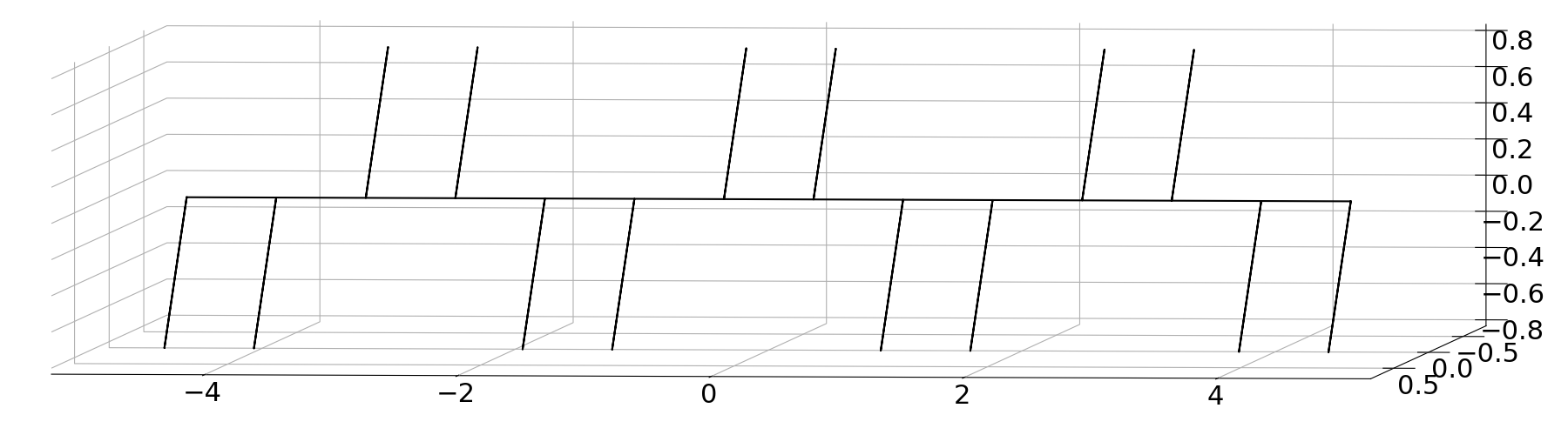
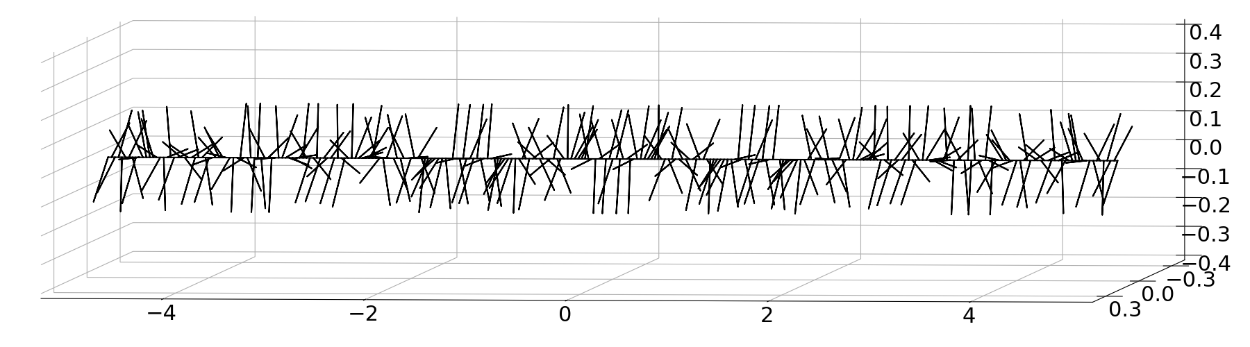
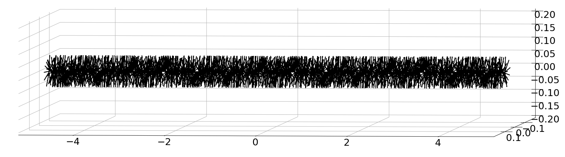
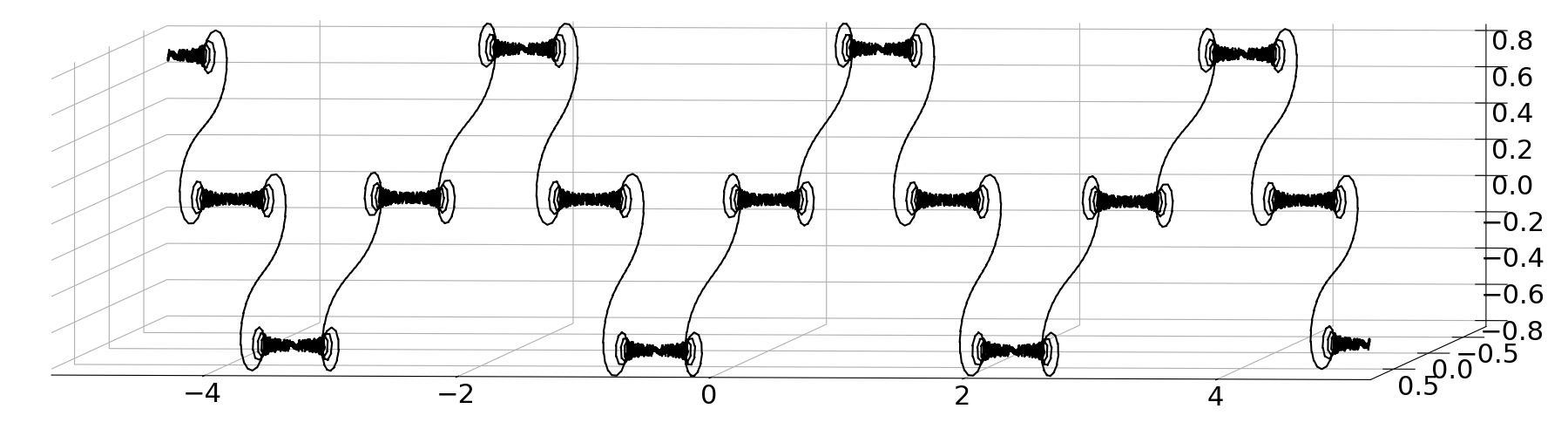
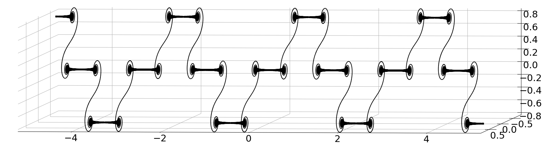
(The choice of is not unique but this does not change the result; see Remark 4.2.) Because of this Gaussian factor, the delta-functions which make up point in many directions in the complex plane, so their sum resembles a brush instead of a comb. (See Figure 1.1.)
Theorem 1.3.
Let and be such that, as in (1.5), for relatively prime and . Let be such that , and let as in (1.6). Recall the definitions of the Dirac comb r in (1.1) and the fractional Fourier transform in Definition 1.1.
Then there exists some such that
| (1.7) |
We separately identify the coefficient in Section 4, which corresponds to the functional equation for Jacobi theta functions as described in Section 3.3.
Theorem 1.4.
The constant in Theorem 1.3 is an eighth root of unity which depends only on and whether modulo 8.
Remark 1.5.
The terms and in (1.7) depend only on the parity of and , since
Furthermore, at least one of and must be even because .
Remark 1.6.
We discuss several symmetries for in Section 4. We note here that the dependence on whether modulo 8 is an ambiguity regarding the sign only, which comes from the fact that while .
We also note that is an even distribution (regardless of whether the support is discrete or not) because r is even and the reflection can be written as which commutes with :
Remark 1.7.
Remark 1.8.
Let us suppose that and are linearly dependent over . To see that (1.5) holds, note that there exist not both zero (and, without loss of generality, relatively prime) such that
| (1.9) |
Consequently, is nonzero (as the product of a two nonzero complex numbers) and real (since the imaginary part vanishes by choice of ). We obtain , allowing us to conclude that (1.5) holds with and . (The fact that follows because .)
1.2. Illustrations of some “Dirac brushes”
To give a concrete example of Theorem 1.3, let and take , so that and . In this case, (see Section 4), and one can compute that
where
We illustrate this distribution at the top of Figure 1.1, where we illustrate functions as curves in .
For comparison, we also illustrate for and (chosen arbitrarily among fractions near ), allowing us to see that the “diameter” and spacing for these brushes, and respectively, tend to zero as becomes large.
Let us consider the third example, where . The result of Theorem 1.3 with , , and , expressed as in (1.8), is
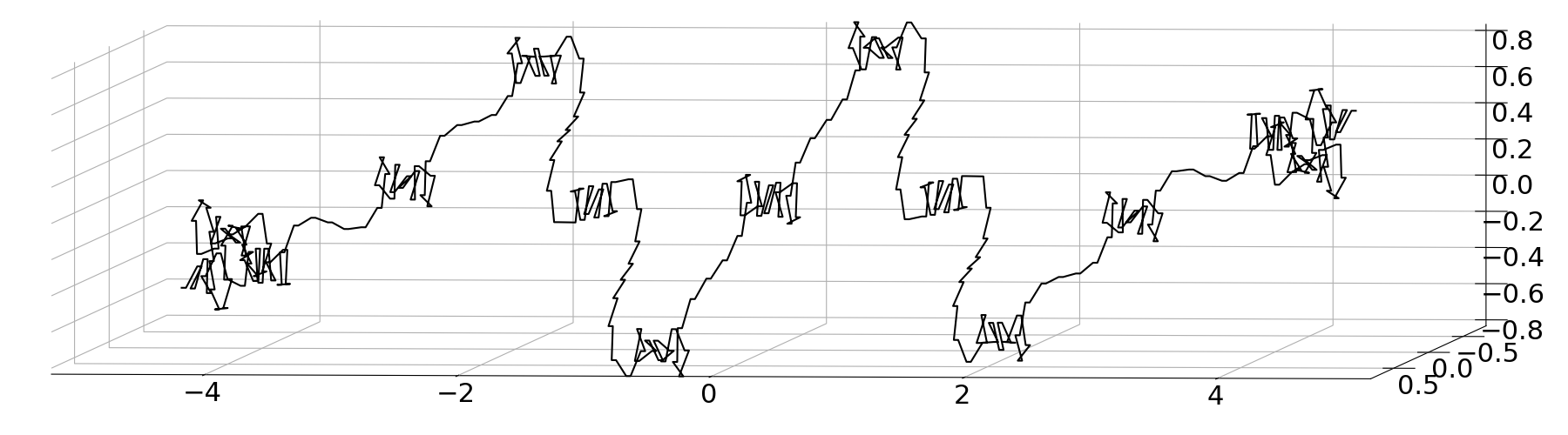
To illustrate that this intimidating expression is far from random (despite appearances in Figure 1.1), in Figure 1.2 we plot the antiderivative
described in Definition 3.7, for the three examples in Figure 1.1 as well as for satisfying . We see that the graphs of and become quite similar to the graph of for , up to a spiraling error discussed in Section 7.3.

1.3. Context and plan of paper
The author has often worked with (complexified) metaplectic operators [14] and happened upon this problem performing some numerical approximations. (It suffices to replace by to obtain super-exponential convergence.) One immediately sees surprising and complicated structure behind the natural question of the interaction between a Dirac comb and the fractional Fourier transform, where the latter can be understood as the Schrödinger evolution of the quantum harmonic oscillator (Remark 3.3).
The objects considered are central to the theory of modular forms, about which the author knows very little. The connection with the metaplectic representation is well-established; see for instance [10]. The author would certainly be interested to find out to what extend this work runs in parallel to (or duplicates) works already established in that domain or elsewhere.
In studying this question, one is naturally led to prioritize the metaplectic representation and its associated (somewhat peculiar) normalizations, already seen in (1.1) and (1.2). As shown in Section 4, the symmetries giving Theorem 1.4 (or, equivalently, the functional equation for the Jacobi theta functions) come from a relatively short list of metaplectic identites. Specifically, one commutes half-integer shifts (2.2) and metaplectic operators (3.3) with straightforward linear algebra, and one can compose metaplectic operators (Lemma 3.14) via their associated linear maps with some occasional sign considerations. The particularities of the Dirac comb appear in the application of integer shifts (2.3), the Poisson summation formula (1.3), and the seemingly elementary fact that because for . Geometrically, this says that a shear in phase space (3.8) acts on the Dirac comb in the same way as a half-integer momentum shift, and this fact alone accounts for all half-integer shifts in the proof of Theorem 1.4.
The plan of this paper is as follows. In Section 2 which follows, we introduce shifts in phase space and their interaction with the Dirac comb and the fractional Fourier transform, and then we prove Theorems 1.2 and 1.3. We introduce the metaplectic point of view in Section 3; this allows us to rephrase Theorem 1.3 in terms of the Dirac comb being an eigenfunction of certain shifted metaplectic operators. We also obtain the relation between Theorem 1.3 and the functional equation for the Jacobi theta functions. In Section 4 we use symmetries given by the metaplectic representation to obtain the coefficient following the algorithm in [12]. In Section 5 we show that, with the Bargmann transform, one can deduce Theorem 1.3 from the functional equation, and we also can establish a type of weak boundedness used later to show weak continuity of the family . In Section 6 we consider periodicity and parity of . Section 7 concerns continuity of : this family is wildly divergent in absolute value in the sense of complex measures, yet continuous when “smoothed” by the harmonic oscillator raised to any power less than . Its antiderivative is not locally uniformly continuous, but we can understand some of its behavior as as approaching Fresnel integrals, and within these Fresnel integrals we can analyze repeating patterns which give the coefficient in terms of Gauss sums. The last section is devoted to the question, not answered here, of what happens when Theorem 1.2 gives : numerically, it certainly seems that the antiderivative converges, but to a rough and possibly self-similar function.
Acknowledgements.
This work began with some conversations during the workshop “Atelier d’Analyse Harmonique 2017” of the ERC FAnFArE. In particular, the author is grateful to Yves Meyer for discussions and encouragement at the outset of this study. The author is greatly indebted to Francis Nier for numerous discussions and helpful references. The author also acknowledges the support of the Région Pays de la Loire through the project EONE (Évolution des Opérateurs Non-Elliptiques).
2. Direct proof of Theorems 1.2 and 1.3
2.1. Shifts in phase space and the fractional Fourier transform
This paper is essentially an application of the theory of metaplectic operators applied to shifts in phase space. Behind all these objects, of course, is the language of symplectic linear algebra, but we minimize the use of this language in the hopes of giving a more approchable presentation.
We define the phase-space shift for as
| (2.1) |
One can readily verify the composition law
| (2.2) |
When , the Dirac comb r in (1.1) is an eigenfunction of with eigenvalue or :
| (2.3) |
Moreover, any distribution such that must be a multiple of the Dirac comb r, a classical fact which we recall in Lemma 3.18 below. In this way, (2.3) defines r up to constants.
2.2. Proof of Theorems 1.2 and 1.3
We now prove Theorems 1.2 and 1.3 using the Egorov relation (2.5) for the fractional Fourier transform. We also use (2.3) and the idea behind the classical Lemma 3.18: when is a distribution and is smooth with simple isolated zeros, implies that is a series of delta-functions supported on .
Proof of Theorem 1.2.
To simplify notation, let us write
so that
Applying (2.5) to (2.3) gives, for any ,
| (2.6) | ||||
For any distribution , . Therefore for every ,
If and are linearly independent over , we can make
arbitrarily small by Dirichlet’s Approximation Theorem (for example, [11, Sect. 1.2]. Furthermore, is a subgroup of that now contains arbitrarily small elements, so it and are dense. Since is closed, we have shown that .
On the other hand, if and are linearly dependent over , as in Remark 1.8 we may choose relatively prime and such that as in (1.5). Replacing with and with and setting in (2.6) gives and
so
Consequently,
which of course implies that is discrete. In fact, because the zeros of are simple, we can conclude from [7, Thm. 3.1.16] that is a delta-function when restricted to a sufficiently small neighborhood of any ; see the proof of Lemma 3.18, which is taken from [7, Sec. 7.2]. Therefore for some sequence of complex numbers,
| (2.7) |
∎
Proof of Theorem 1.3.
3. Using the metaplectic representation of
3.1. Introduction to metaplectic operators
The fractional Fourier transform is but one of many metaplectic operators (we restrict our discussion to dimension one except for Section 4.2), a closed subgroup of unitary operators on which are automorphisms of and which preserve linear forms in . (See, for instance, [9].) They are in two-to-one correspondence with matrices with real entries and determinant one,
| (3.1) |
and when (we postpone the case for Remark 3.1), we may write the integral kernel for as
| (3.2) |
We adopt the convention that the sign of the square root is such that , but is also a metaplectic operator, and and are the only metaplectic operators associated with .
Our principal tool linking metaplectic operators and shifts in phase space is the (exact) Egorov relation
| (3.3) |
It is elementary to confirm this from the integral kernel (3.2); we omit the moderately lengthy computation.
The metaplectic group is generated by , scaling, and multiplication by Gaussians with imaginary exponents; we define these two last families now.
For ,
| (3.4) |
is clearly unitary on . It also induces, in the sense of (3.3), the transformation
| (3.5) |
It is, in fact, through the scaling that we have defined the comb r in (1.1): because a -function is homogeneous of degree ,
| (3.6) |
For , we also have
| (3.7) |
which induces the transformation
| (3.8) |
Remark 3.1.
We can now describe when the upper-right entry of is zero. In this case we must have, for some choice of sign making ,
When the sign is positive,
When the sign is negative, since we can write
The choice to use instead of is completely arbitrary and has no deeper significance.
Remark 3.2.
If is the integral kernel of , notice that . For this reason, when is the sesquilinear dual bracket between and , we still have
Therefore (so long as both members are in or one is in and one is in ) we treat all inner products like across which the “unitary” operators and may be passed.
Remark 3.3.
The generators of the metaplectic representation are the Schrödigner evolutions of certain degree-two polynomials in
The infinitesimal generator of the family of fractional Fourier transforms is the quantum harmonic oscillator
| (3.9) |
meaning that
| (3.10) |
in the sense that
for all .
It is quite elementary to see that the infinitesimal generator of is in the same sense, since
The scaling can be written using
where the term comes from the Weyl quantization. Specifically,
and one could therefore make the case that is more natural to use as appears elsewhere in the literature. The author feels, in the end, that the current definition of is perhaps more familiar.
Similarly, shifts in phase space are also Schrödinger evolutions, in the sense that
This may be checked directly or found in essentially any discussion of the Weyl quantization.
3.2. Restatement and proof of Theorem 1.3
We rephrase Theorem 1.3 in terms of metaplectic operators since this simplifies the proof of Theorem 1.3 significantly and lays the foundation for identifying the coefficient . On the other hand, the factor appears as a deus ex machina.
Using the metaplectic definition presented in (3.6), from (3.7), and shifts from (2.1) which satisfy (2.3), Theorem 1.3 becomes
We can solve for 1 on the right, obtaining
A straightforward computation, presented in Lemma 3.10, shows that under the hypotheses of Theorem 1.3 and when ,
| (3.11) |
Conversely, allowing for any and varying choices of (Remark 4.2), every for can be obtained in this manner.
Of course, is an eighth root of unity. We may also, remaining within the set of eighth roots of unity, replace by any other with the same parity, since by (2.2) and (2.3), whenever ,
| (3.12) | ||||
We therefore rephrase, and prove, Theorem 1.3 in the following equivalent way.
Theorem 3.4.
Let , and let . Recall the definitions of the Dirac comb 1 in (1.1), the shift in (2.1), and the metaplectic operator in (3.2) or in Remark 3.1.
Then there exists for which
| (3.13) |
if and only if and if .
Remark 3.5.
Proof.
Using (2.3), the Egorov relation (3.3), and (2.2), for any
where is not used here. Therefore if (3.13) holds, then for any
which can only hold if for all . (If not, will not be supported in or will not be -periodic.) Therefore is a necessary condition for (3.13).
Let us suppose then that . By the classical Lemma 3.18, it is enough to show that
is invariant under and . Using (2.2), (3.3) where we apply , and (2.3),
Similarly,
We see that is invariant under and if and only if if and only if ; therefore, when this holds, it is a multiple of the Dirac comb 1. Since the multiple cannot be zero since is invertible on , this proves the theorem. ∎
Remark 3.6.
Having defined in Theorem 3.4, we record the equivalent formula for in terms of a sum of -functions. Recall that we assume that for relatively prime and , that are such that , and that . Fix such that , and let . To handle , we simply let if and otherwise. We then solve for in
to obtain
Definition 3.7.
Taking for simplicity, when and are linearly dependent over , we define the antiderivative for as
More precisely, since -functions are involved,
We extend to be an odd function, so in particular .
For example, with this definition, if for , then , and for all .
The advantages of this definition are that should be an odd function, since is even (Remark 1.6) and that .
3.3. And the functional equation for theta functions with half-integer characteristics
The Jacobi theta functions can be obtained by taking the duality product of Gaussians and (shifted) Dirac combs. Let
and
| (3.14) | ||||
When and , we write
| (3.15) |
This notation differs slightly from the notation used in [12] but agrees for , and and agrees more generally up to eighth roots of unity.
Testing Theorem 1.3 against Gaussians gives the classical functional equation [12, Thm. 7.1] for Jacobi theta functions, which describes the transformation of these theta functions under the action of . Or, if the reader prefers, the identification of as an eighth root of unity is a consequence of this classical functional equation.
Theorem 3.8.
Proof.
Remark 3.9.
This presentation of the functional equation for the Jacobi theta functions allows us to identify certain separate “moving parts.” Most importantly, the eighth root of unity belongs to the Dirac comb and its transformation under metaplectic operators, and it has nothing to do with or . The linear fractional transformation giving from and the factor are due to the transformation of a (centered) Gaussian under a metaplectic operator.
Finally, the formula for and the factor comes first from the metaplectic operator, which transforms into , and then from our insistence that the shift is of the form , in momentum only. This (somewhat unnatural) requirement leads us to project onto along , which explains the dependence of on as well as the factor . (See Lemma 3.13.) One could naturally simplify this dependence in defining for and the function
for which
But, of course, one could eliminate and as well by writing Theorem 3.4.
3.4. Lemmas on the metaplectic operator
In this section, we collect a number of elementary lemmas on metaplectic operators and their effect on Gaussians. The results of principal interest are (3.11) relating Theorem 1.3 to Theorem 3.4 and the effect of a metaplectic operator on a Gaussian.
Lemma 3.10.
Proof.
We use the Mehler formula (1.4); the case , when , is trivial because and . Along with the change of variables , we obtain
It suffices to show that the coefficient of in the exponent is in fact . Using ,
This confirms that the coefficient of is and completes the proof of the lemma. ∎
In order to compute the effect of a metaplectic operator on a Gaussian
we begin with the centered Gaussian .
Lemma 3.11.
Let and suppose that . Let . Define
Then, with the metaplectic operator defined as in (3.2),
where the square root is chosen such that .
Proof.
This is a direct computation:
We check the sign of the coefficient: in order to integrate the Gaussian, we have used that
where . The square root is therefore chosen such that
Because is defined with , meaning that , we have that
Therefore
with positive real part.
The coefficient of in the exponent is
because . This completes the proof of the lemma. ∎
Remark 3.12.
For any with fixed, the set of Gaussians has dense span in ; indeed, if for all , a modified Bargmann transform of , like the one used in Section 5, vanishes identically. The relation
coming from the Egorov relation (3.3) and Lemma 3.11, therefore suffices as a definition of . Note that this definition does not require , but the choice of sign when and is still somewhat arbitrary.
However, there is some ambiguity in that many different give, up to constant multiples, the same . These are equal modulo the plane associated with the Gaussian ; see [6, Sect. 5].
Lemma 3.13.
Let and let . Then there exists such that
if and only if . In this case, .
Proof.
It is instructive to begin with the case , where it is evident that
if and only if (and in this case the constant is ).
The general result follows from writing the equivalent statement
and applying the previous special case. ∎
A consequence, which may be checked directly, is that, when and if and ,
| (3.17) |
As an application of the effect of a metaplectic operator on a Gaussian, we finish this subsection by proving some well-known formulas for compositions of metaplectic operators.
Lemma 3.14.
Let for with
Then there exists a such that
For any with ,
where each of the three terms has positive real part.
Corollary 3.15.
The set is closed for any subgroup of .
Proof.
In view of the density of (see Remark 3.12), it suffices to show that and agree on any Gaussian . When
and when ,
Since , it suffices to show that and that we have the correct formula for .
Expanding
we compute
and
Therefore and
as promised. It is clear that and that is a continuous function of to , so is independent of and the lemma is proved. ∎
In the case of scaling or multiplication by a Gaussian, , which may also be easily verified using the integral kernel.
Proof.
In the former case, , we have and , and in the latter case, , we have and . It is obvious, in either case, that in Lemma 3.14. ∎
Remark 3.17.
Having established composition rules for metaplectic operators, we note that Lemma 3.10 follows upon checking that which is an elementary matrix multiplication.
3.5. Identification of r via invariance under integer shifts
We record the classical fact that the Dirac comb r from (1.1) is the only distribution (up to constant multiples) invariant under both and . The proof is adapted from [7, Sec. 7.2].
Lemma 3.18.
A distribution is a constant multiple of the Dirac comb r in (1.1) for if and only if
| (3.18) |
Proof.
Writing using the definition (1.1) gives the equivalent statement
This is true by a change of variables and by the observation that when for any .
Suppose, conversely, that the two equalities in (3.18) hold. When , . Therefore and, since the zeros of are nondegenerate, in a neighborhood of any ,
Therefore, by [7, Thm. 3.1.16], coincides with a multiple of a function in a neighborhood of any , or
for some sequence of complex numbers. Finally, , so is -periodic. Therefore is a constant sequence and . ∎
4. Evaluation of the coefficient
We follow [12] in showing that the coefficient in Theorem 3.4 can be obtained from certain symmetries. We remark that, when is the identity matrix and , then is the identity operator, and by (2.3),
We also note that changing representations of modulo 2 follows readily from (3.12): by Theorem 3.4, when ,
By (3.12),
so, still supposing that ,
| (4.1) |
We therefore search for symmetries paying little regard to . Following the proof of [12, Thm. 7.1], it is enough to understand how changes under the transformations
Here, the matrices and (where ) are defined in (2.4) and (3.8). The effect of these transformations on follow from the Poisson summation formula and the effect of multiplication by Gaussians on .
Proposition 4.1.
Proof.
For the first, we revert to the expression corresponding to Theorem 1.3 via Lemma 3.10. Specifically, with and when for ,
| (4.2) |
By the Poisson summation formula (1.3), . Note that and is unchanged under replacing with . However, if and , then is no longer in . To correct for this, we replace by . Therefore
and (4.2) becomes
proving the first equality in the proposition.
For the second and third equalities, we use the observation that
| (4.3) |
with the multiplication operator defined in (3.7) and from (3.8). Notice that, unlike composition with the Fourier transform, there is no change of sign; see Corollary 3.16.
By the definition of in Theorem 3.4, the first equality in (4.3), and the Egorov relation (3.3) for and ,
In order to cancel , we observe that
| (4.4) |
because for . Therefore , and our computation becomes
by the composition law (2.2). By the definition of in Theorem 3.4, this proves
and therefore the second equality in the proposition.
Remark 4.2.
Another view of the second equality in Proposition 4.1 is that multiplying by is equivalent to changing the choice of in Theorem 1.3. Indeed,
and replacing by in Theorem 1.3 (taking for simplicity) is possible if and only if , meaning that for some because and are relatively prime. In this case, , in correspondance with the second equality in Proposition 4.1.
Remark 4.3.
There are many symmetries which we do not use in proving the functional equation. One worth remarking on is
which follows immediately from the fact that whenever is real-valued, and as well. This allows us to compute for any real-valued (see Remark 3.2)
This corresponds to the symmetry
4.1. Algorithm to identify
We recall the method in the proof of [12, Theorem 7.1] to identify the coefficient in the functional equation for the Jacobi theta function, adapted for our setting.
Let be such that and . We can choose such that ; we apply the third equality in Proposition 4.1 to replace with . The first equality (the Poisson summation formula) allows us to replace with , and we continue until . In this case , so we can replace with by multiplying by in view of (4.1). Finally, the observation (4.4) and for all gives for all and . Applying the first equality of Proposition 4.1 twice gives that . This gives us the value of .
To make this procedure concrete, we present it in a few lines of code in Python, which returns such that .
def logmu(a,b,c,d,q,p):
K = 0
while b != 0:
j = -a//b
K = K + j*(d*q - p*b) Ψ# Third equality
a, c, p, q = a+j*b, c+j*d, q-j*b, p-j*d Ψ# Third equality
if a < 0 and b >= 0:
K = K - 3 Ψ# First equality, sigma = -1
else:
K = K + 1 Ψ# First equality, sigma = +1
a,b,c,d = -b,a,-d,c Ψ# First equality
K = K+p*q Ψ# Reduction from (q, p) to to (0, q)
if a == -1:
K = K - 2Ψ# If a = d = -1
return(K%8)
4.2. A remark on higher dimensions
We have focused here on dimension one because there is a natural continuous one-parameter group of transformations that the author wishes to study. When rephrased in terms of the metaplectic representation of , very little changes in higher dimension. We describe the analogous result rapidly without attempting any deeper study.
In this section, is the dimension and
We recall that is the set of linear transformations of leaving invariant the symplectic form
(so if for all ). Shifts are defined identically,
One has the composition law and that whenever .
When
for , and when , we may similarly define the metaplectic operator
(where the author has no preferred choice of sign for the square root). When one may concoct a composition of multiplication by Gaussians with imaginary phase and changes of variables. One may alternatively view the metaplectic representation through its generators: the Fourier transform in the first variable, changes of variables, and multiplication by Gaussians with imaginary phase (see for instance [8, Lem. 18.5.9]). As a final approach, one may define a metaplectic operator through its effect on Gaussians as in Remark 3.12.
With any approach, one has a family of operators corresponding two-to-one with ; these operators are unitary on , isomorphisms of and , and the Egorov relation
We simply record that an obvious analogue of Theorem 3.4 holds in any dimension.
Theorem 4.4.
For , let . Define as the scalar product of the -th rows of and of (equivalently, the -th diagonal entry of ) and let be the scalar product of the -th rows of and of . Let and let . Then, when , when is the corresponding shift operator, when is one of the two metaplectic operators corresponding to , and when 1 is the Dirac comb, there exists such that
| (4.5) |
if and only if , and in this case .
Proof.
Let be the basis vector which has zeros for entries except for a one in the -th position. Just as in the proof of Theorem 3.4, following [7, Sec. 7.2], existence of follows from showing that
for .
We compute using the Egorov relation that
where and is the -th column of . Since , we can write [10, Sect. 1.1.9]
When and are the entries of and ,
and, since was defined to be ,
The fact that follows from the fact [12, Prop. A 5] that is generated by
where and is symmetric. These correspond to the Fourier transform, changes of variables , and multiplication by Gaussians with imaginary phase . The Fourier transform gives an eighth root of unity by the Poisson summation formula, and the changes of variables give fourth roots of unity (depending on the choice of signs for square roots) because .
Multiplication by Gaussians corresponds to a half-integer shift: when is the diagonal of ,
This is because is symmetric and, for ,
so
As in dimension one, commutators and compositions of half-integer shifts produce eighth roots of unity (and only eighth roots of unity).
Having shown that generators of the metaplectic representation, when composed with appropriate half-integer shifts, act on the Dirac comb by multiplication by eighth roots of unity, we have proved the theorem. ∎
5. The Bargmann transform
The Bargmann transform [4]
| (5.1) |
plays a central role in the analysis of the quantum harmonic oscillator defined in (3.10). (A good reference is [5, Chap. 1.6].) The Bargmann transform, which can be formally viewed as the metaplectic operator associated with
| (5.2) |
is a unitary map from to the space of holomorphic functions for which
is finite. In this section, we show that the Bargmann transform allows us to prove Theorems 1.3 and 1.4 as a consequence of the classical functional equation in Theorem 3.8. As in Section 2.2, we write
| (5.3) |
Supposing that and are linearly independent over , we write for linearly independent and (Remark 1.8).
Our goal being to present the proof as rapidly as possible, we restrict ourselves to the case where and where and are both even. In this case, Theorems 1.3 and 1.4 reduce to the existence of some for which and
| (5.4) |
We leave it to the interested reader to extend the computation to general (which is quite straightforward) and general such that , which can be done using symmetries of theta-functions as in [12, Table 0, p. 19]. We also rely on direct computation; applications of the metaplectic theory, while clearly interesting to the author, are presented elsewhere in this work.
Conjugation by simplifies the harmonic oscillator because
| (5.7) |
and therefore, recalling (5.3) and using the shorthand ,
| (5.8) |
The former equality follows from direct computation or an Egorov theorem for Weyl quantizations; the latter can be seen because the problem is easy to solve. (See for instance [2, 3].)
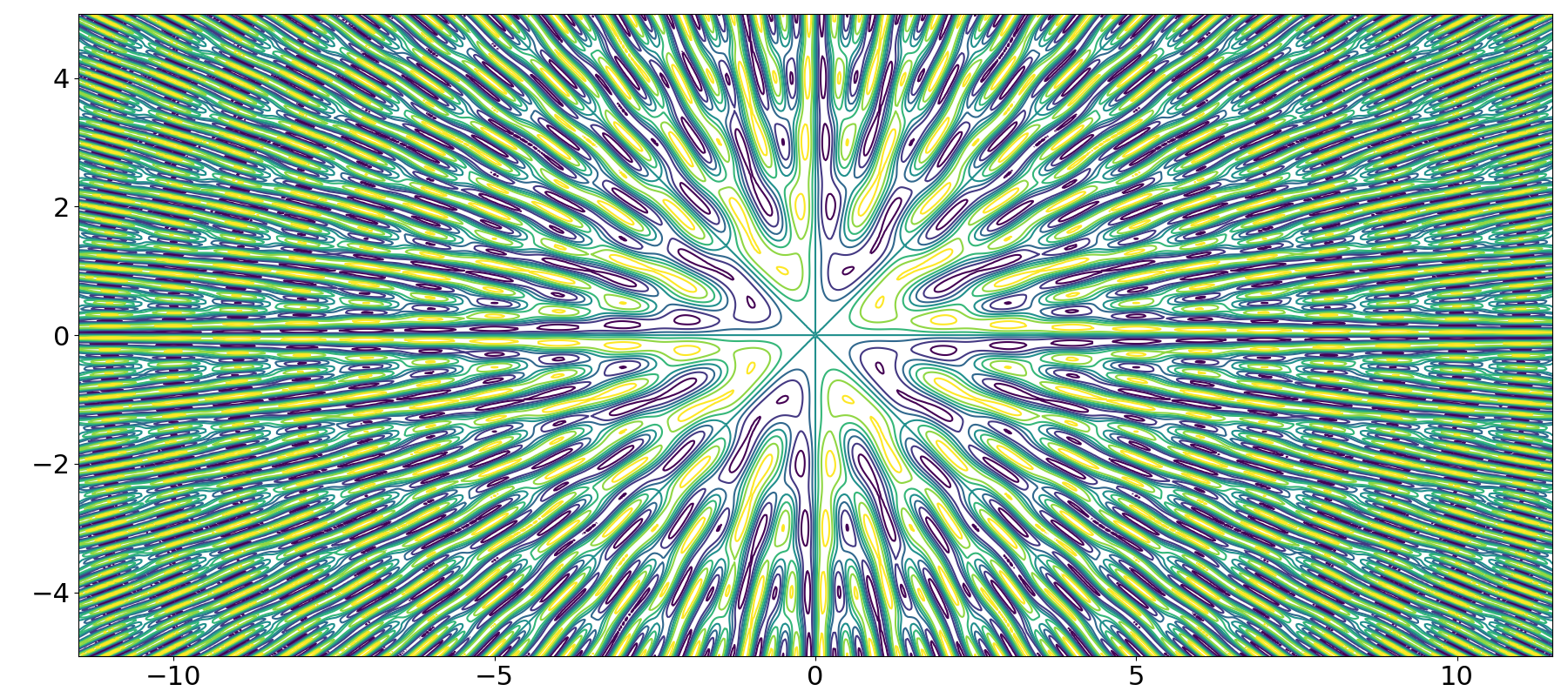
In Figure 5.1 we draw contours of the imaginary part of the normalized Bargmann transform ; this is normalized in the sense that
Note that this function is bounded by Proposition 5.2. By (5.8), we are, in effect, studying symmetries under rotation of this function.
Example 5.1.
We apply the (unitary) Bargmann transform to (5.4). Applying (5.8) to (5.5) for the left-hand side and using (5.6) as the right-hand side, we see that Theorem 1.3 (for and even) is equivalent to
Setting , we rewrite this equality as
| (5.9) |
To see that this is a consequence of the classical functional equation presented in Theorem 3.8, we analyze , , and . Recalling that ,
Next,
Finally, using that ,
These three computations, when inserted into (5.9), give that Theorem 1.3 for and even is equivalent to
This, in turn, is a special case of the well-known Theorem 3.8.
An observation, useful in controlling the regularity of r (Proposition 7.2), is that the Bargmann mass is bounded. This follows from the fact that it is a smooth periodic function.
6. Periodicity and parity
In Section 8 we observe (without proof) that approximations to when seem to be at many points nearly periodic, nearly odd, or nearly even. In this section, we consider when is exactly periodic, exactly odd about a point, or exactly even about a point, which is significantly more restrictive.
6.1. Periodicity and crystalline measures
To better understand , a natural question is whether this function is periodic, as for instance plainly is (Figure 1.1). Another natural question is whether is a crystalline measure, meaning that the support of it and its Fourier transform are both discrete. We group these two questions together because the answers are the same.
Proposition 6.1.
Proof.
The distribution is periodic if and only if there exists some such that
By the Egorov relation (3.3) for given by (2.4), this is equivalent to
Since we may eliminate the operator from both sides, this is possible if and only if
| (6.1) |
for for which is even; see (2.3). Because
so has discrete support by Theorem 1.3.
Conversely, if has discrete support, then by Theorem 1.2 and Remark 1.8, there exists such that
By the preceding discussion, in particular (6.1), this means that is periodic with period .
Finally, if , then has discrete support if and only if , by Theorem 1.2. In this case, is discrete if and only if
which holds if and only if . ∎
6.2. Parity
A function is even/odd at if is even/odd, meaning that . Recalling that , we say that a Schwartz distribution is even/odd at if
Take . As usual, write , and recall the Egorov relation . We also use that r is even in computing
Recalling (2.3), we obtain the following proposition.
Proposition 6.2.
Let and write for . Let be the fractional Fourier transform of the Dirac comb. Then is even or odd around if and only if
and in this case is even if is even and odd if is odd.
Example 6.3.
If then . Then is even at if and only if and odd if and only if . This agrees with the formula identified and illustrated in Section 1.2.
7. Questions of continuity in
The most interesting aspect (to the author) of the study of the fractional Fourier transform of Dirac combs is the question of how the result varies as varies.
As we will discuss, it is obvious that the function is far from being absolutely continuous from to the set of measures, and it is obvious that it is continuous from to .
We show that the function is continuous from to for any , the image being essentially a Sobolev space defined by the quantum harmonic oscillator instead of .
We also show that the antiderivative (Definition 3.7) is not locally uniformly continuous in . It has, however, a particular behavior as in certain regimes: the antiderivative tends to a rescaled Fresnel integral, leading to the appearance of Euler spirals when the values of are traced in the complex plane.
Within these Euler spirals one observes repeating motifs depending on if and . We show that these repeating motifs are the graphs of Gauss sums, and one can use this observation to express the eighth root of unity in Theorem 1.4 via a Gauss sum (which is classical in the study of theta functions).
7.1. Lack of absolute continuity
It is obvious that the absolute value of the (when we can describe this measure via Theorems 1.2 and 1.3) diverges wildly. It suffices to observe that when as in (1.5), the absolute value (in the sense of measures) of is
which charges an interval of length with a mass of (up to the obvious rounding error depending on exactly where the endpoints of the interval fall). Because is finite for any , we have the following proposition on divergence of the absolute value of (which applies equally well to any for fixed).
Proposition 7.1.
For any open set and for any , the number of such that and are linearly dependent over and for which
is finite.
7.2. Weak continuity in
When the quantum harmonic oscillator defined in (3.9), we recall that the Schwartz space is simply
with the associated family of seminorms. Since is a function of , it is obvious that preserves the seminorms of . Because , by duality it is clear that is continuous from to .
We would like to have more precise information on how much regularity (and decay) is required to make continuous in .
Proposition 7.2.
Remark 7.3.
For brevity, we will use the Bargmann transform to control , using methods similar to those in [2, 3]. An alternate proof, omitted here, is to explicitly compute using the Mehler kernel. For small , one obtains an almost orthogonal family of Gaussians and the sum of the norms gives the somewhat sharper estimate
from which one can deduce the result.
Proof.
Because , we have that acts continuously on and therefore on which contains r. If is such that the integral converges absolutely,
| (7.1) |
If , this comes from
and for general functions this comes from the decomposition of into (Hermite) eigenfunctions of .
It therefore is enough to control which is in when .
Conjugating by the unitary Bargmann transform, we obtain via (5.7) and (5.8) that
Because (Proposition 5.2) and because
we see that there exists some constant such that
Therefore
Since when is small and when is large, the last integral is finite if and only if . This proves the proposition. ∎
Corollary 7.4.
Let and define, where possible,
If there exists some such that , then is continuous on . If there exists some such that , then is on . If there exists some such that , then is analytic on .
7.3. The limit , Fresnel integrals, and Gauss sums
Numerical computation quickly reveals that the antiderivative
defined in Definition 3.7 does not, as within , tend locally uniformly to
Some further analysis reveals that the rescaled resembles the Fresnel integral
| (7.2) |
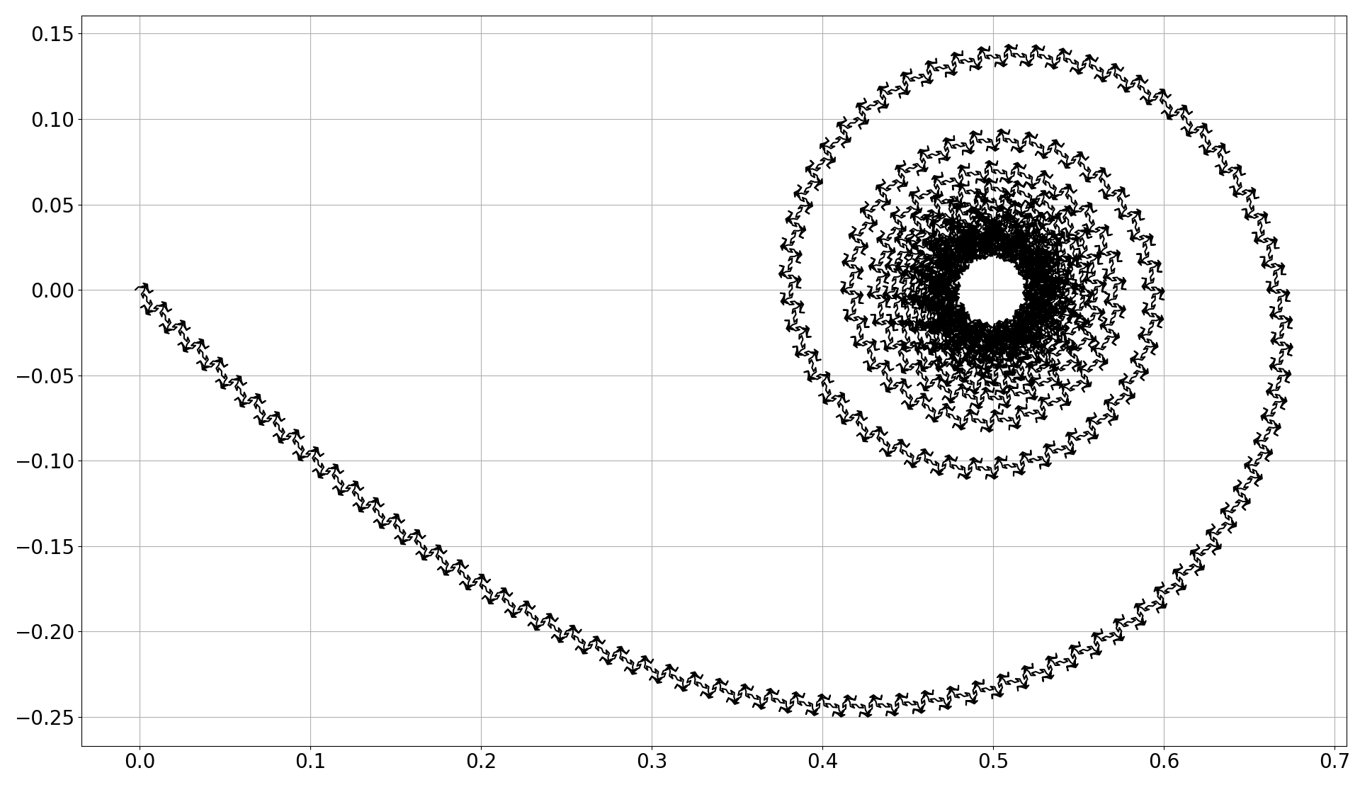
Morever, when with (relatively prime integers) and , the spiral traced by the values of in the complex plane is made up of small repeating blocks which depend only on and on . (See Figure 7.1.) These blocks correspond to certain Gauss sums, and analyzing these motifs allows us to deduce an expression for the eighth root of unity in terms of these Gauss sums. We note that the case is the complex conjugate of the case ; see Remark 4.3.
Our goal is to establish this expression in the following form.
Theorem 7.5.
7.3.1. Decomposition of
We study , when with are relatively prime, by studying when and in .
We therefore fix with and . We write as in Theorem 3.4. Following Proposition 4.1, we let
and we have
The sum in Remark 3.6, using Proposition 4.1, is
when is defined by removing the principal part, , of ,
and is what remains in the exponent,
| (7.3) |
We compute that
We will show in Lemma 7.7 below that, when is a generic element of , the function is independent of in , is -periodic in modulo , and can be expressed as
Therefore, for all . In particular, we can express in a unique way as
and when is defined by or
we obtain
It is convenient to introduce
| (7.4) | ||||
which are functions of and . We record the asymptotics that
We also introduce notation for the inner sum above, which as we will describe is essentially a discrete approximation to a Fresnel integral:
| (7.5) |
We remark that we may write using shifts and metaplectic transformations as in (2.1) and Section 3.1:
| (7.6) |
Proposition 7.6.
Then, with and defined as in (7.4) and ,
Lemma 7.7.
The function
with defined in (7.3) is independent of and -periodic as a function from to ; it is given by the formula
Proof.
We expand to obtain
Since ,
is -invariant. (One may also recognize the form of a shift, in this case by , being projected onto along the Lagrangian associated with , as in Lemma 3.13.) Therefore
Recalling the Gaussian defined in (3.14), we obtain, through Lemma 3.13 or through direct computation,
As for periodicity, we compute
To show that for , it suffices to show that is even. We recall that at least one of and is even, since and . If both and are even, then cannot be odd because then both and are even, contradicting . If is odd then is even and is odd, so is even. The corresponding reasoning — if is odd then is even and is odd, so is even — completes the study of different cases. We conclude that is -periodic when viewed as a function from to . ∎
7.3.2. Proof of Theorem 7.5
We can analyze the “Riemann sums” either using standard results of numerical integration (to justify images like the one in Figure 7.1) or by testing against a Gaussian. The latter approach turns out to be significantly simpler, which is to be expected because it fits naturally with the metaplectic representation. In both approaches, however, we obtain the same scale: the Fresnel integrals live on a scale , so to capture enough information we need to take . On the other hand, we surely cannot expect to take or even , because the antiderivative of weakly approaches , the antiderivative of 1, and jumps from on the interval to on the interval .
In terms of testing against a Gaussian , this forces us to choose and , which we express in terms of as follows.
Proposition 7.8.
Proof.
We use the metaplectic presentation in (7.6), as well as unitarity of metaplectic transformations (Remark 3.2) and the Poisson summation formula. Letting
we compute
The Fourier transform of for is ; since we choose , we have . We compute
Under our hypotheses, when , then . Furthermore, as , so because , as . Therefore
because, as , the terms in the sum where are superexponentially small. ∎
This allows us to prove Theorem 7.5.
Proof of Theorem 7.5.
Let and be as in (7.4) and let be such that yet . (If one wishes to be concrete, let , so that “lives on” .) By Propositions 7.6 and 7.8,
On the other hand, since
one obtains using Lemma 3.11 that
Since and , and as . Having also assumed that ,
This shows that
Since , this completes the proof of the theorem. ∎
7.3.3. Riemann sums for the Fresnel integral
The antiderivative of defined in 7.5 is
| (7.7) |
We may take without loss of generality. (Strictly speaking, to match the antiderivative defined in Definition 3.7 we should take the mean of the sum over and the sum over , but the error is bounded by .)
Fix an order as well as , , and a number of intervals . Let and . A straightforward consequence of the Newton-Cotes formulas is that there exists a such that, for any which is times continuously differentiable,
We apply this to , where and the derivative is bounded by . The rounding error where is absorbed in , and we obtain for ,
Our application will be to and . In this case, a simple consequence of the estimate above is the convergence of to a Fresnel integral when and , uniformly in the following sense.
Proposition 7.9.
Let be as in (7.7) and fix any . If as then
Proof.
Under these hypotheses,
which tends to zero as and . ∎
Corollary 7.10.
Fix relatively prime integers with and let be such that . For any , the antiderivative (Definition 3.7) converges to the rescaled Fresnel integral
uniformly on in the sense that
Proof.
Remark 7.11.
In particular, because
we do not have uniform convergence of to in any neighborhood of zero. We do, however, have “uniform convergence” to in the obvious sense on intervals for fixed.
Remark 7.12.
Uniform estimates as (instead of for as ), estimates for in larger sets, or statements of pointwise convergence would certainly be interesting, and seem numerically to be plausible. The author does not currently have any results in these directions.
8. Numerics around approximations to irrational cotangents
The list of things that the author does not know about is enormous. Here, we focus on the question of what happens when is irrational. Indeed, this work fails to answer the second most natural question about : having identified , what is ?
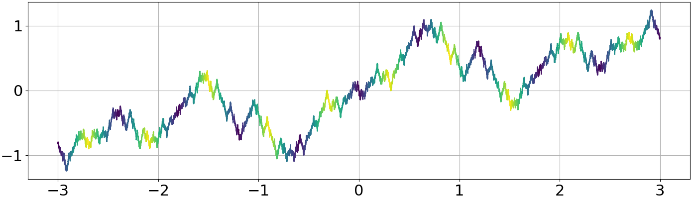
We have already seen (Figures 1.1 and 1.2, Section 7) that the antiderivative appears to better show continuity in . It is straightforward to compute when is a (continued fraction) approximation to . A very striking way to consider these approximations, presented in Figure 8.1, is via the values of the antiderivative in the complex plane. This flattens the depth , so we use varying colors (oscillating between yellow and dark blue) to indicate this change. In particular, this also helps to see where the path re-crosses itself (frequently), giving information which would be lost with a monochrome curve. To try to clarify this approach, we include in Figure 8.2 the real and imaginary parts of for an approximation .
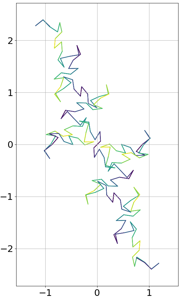
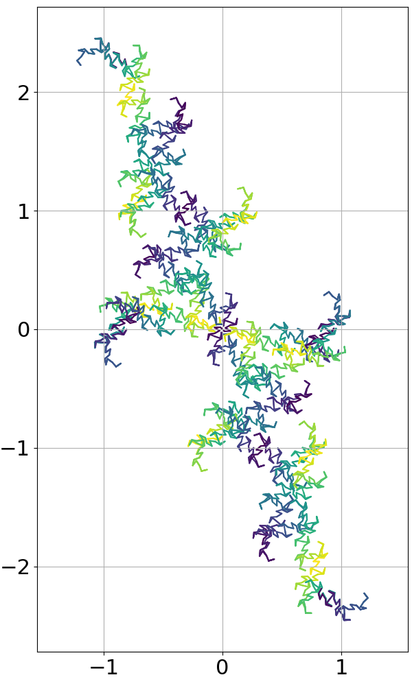
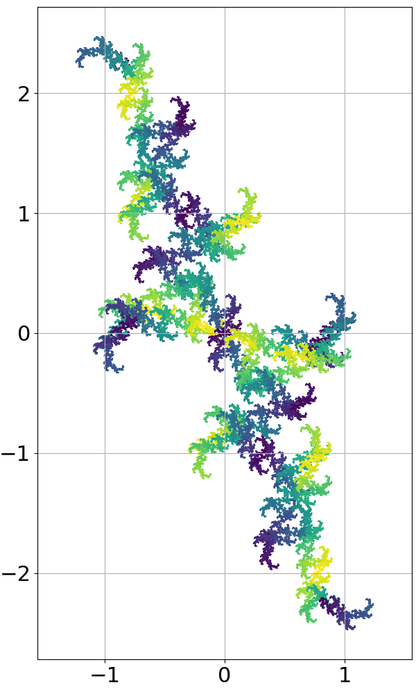
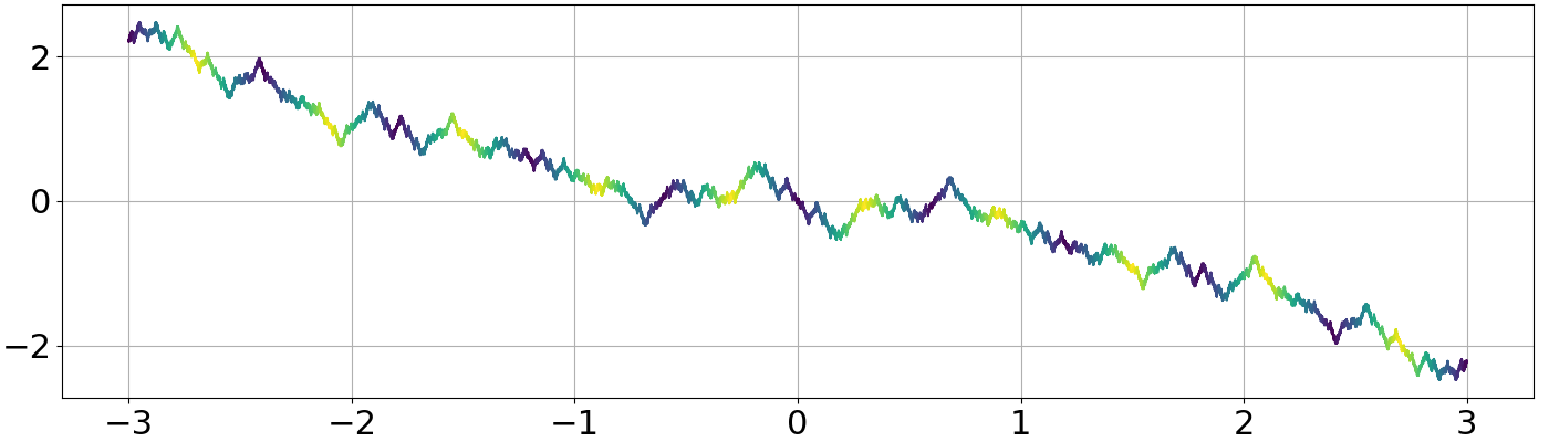
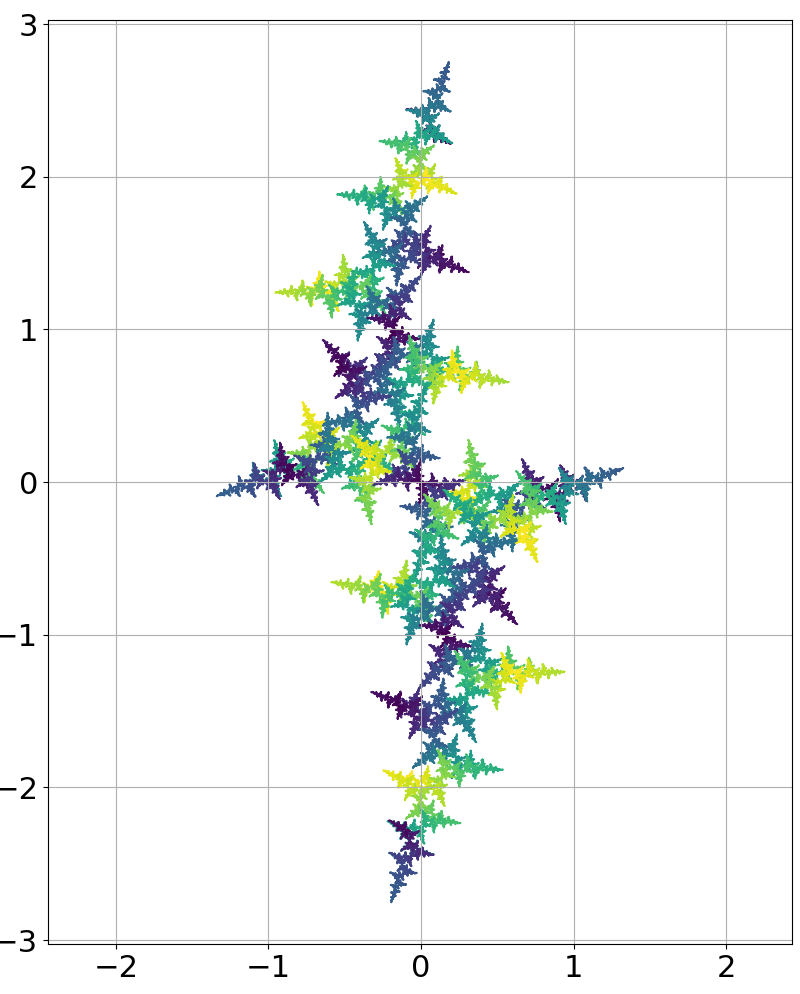
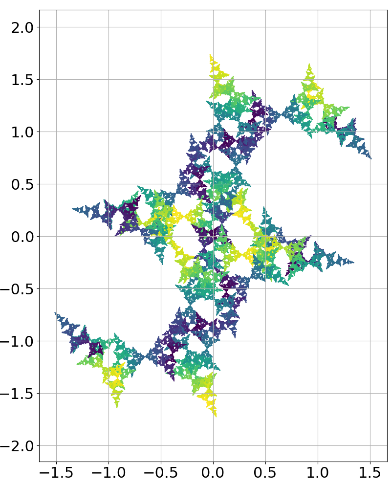
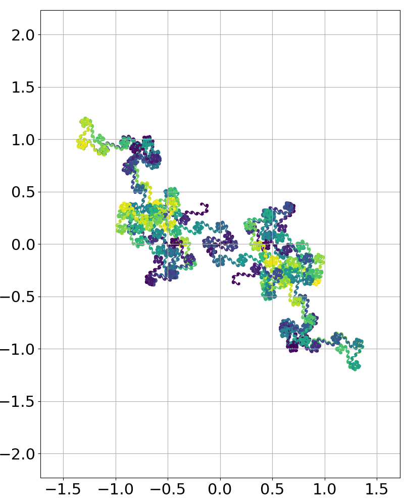
To the naked eye, it certainly seems that there is a limit which is a continuous but not differentiable function whose weak derivative gives .
In Figure 8.3 we draw the values of for similar approximations to cotangents , , and . The square roots (with their repeating continued fractions) appear to have striking self-similar polygonal structure, and the graph of the values corresponding to seems to contain Euler spirals on several scales (which seem to correspond to large denominators in the continued fraction expansion).
Though we know that these functions are neither even nor odd around any point (Proposition 6.2), it certainly appears that there are many around which these approximations are nearly and locally even or odd.
One could also wonder whether the is Hausdorff continuous (if it is a function), whether the image has Hausdorff dimension larger than one as a subset of , whether these functions are nearly periodic and in what sense, whether parts of these curves are self-similar under scaling, what the behavior is as , and on and on.
At present, the author has very few answers. The questions seem quite natural, nontrivial, and, in the author’s opinion, beautiful. The author hopes that, through further study or through exchange with other areas of research, more information will come to light.
References
- [1] Milton Abramowitz and Irene A. Stegun. Handbook of mathematical functions with formulas, graphs, and mathematical tables, volume 55 of National Bureau of Standards Applied Mathematics Series. For sale by the Superintendent of Documents, U.S. Government Printing Office, Washington, D.C., 1964.
- [2] Alexandru Aleman and Joe Viola. Singular-value decomposition of solution operators to model evolution equations. Int. Math. Res. Not. IMRN, 2014.
- [3] Alexandru Aleman and Joe Viola. On weak and strong solution operators for evolution equations coming from quadratic operators. J. Spectr. Theory, 8(1):33–121, 2018.
- [4] Valentine Bargmann. On a Hilbert space of analytic functions and an associated integral transform. Comm. Pure Appl. Math., 14:187–214, 1961.
- [5] Gerald B. Folland. Harmonic analysis in phase space, volume 122 of Annals of Mathematics Studies. Princeton University Press, Princeton, NJ, 1989.
- [6] Lars Hörmander. Symplectic classification of quadratic forms, and general Mehler formulas. Math. Z., 219(3):413–449, 1995.
- [7] Lars Hörmander. The analysis of linear partial differential operators. I. Classics in Mathematics. Springer-Verlag, Berlin, 2003. Distribution theory and Fourier analysis, Reprint of the second (1990) edition [Springer, Berlin; MR1065993 (91m:35001a)].
- [8] Lars Hörmander. The analysis of linear partial differential operators. III. Classics in Mathematics. Springer, Berlin, 2007. Pseudo-differential operators, Reprint of the 1994 edition.
- [9] Jean Leray. Lagrangian analysis and quantum mechanics. MIT Press, Cambridge, Mass.-London, 1981. A mathematical structure related to asymptotic expansions and the Maslov index, Translated from the French by Carolyn Schroeder.
- [10] Gérard Lion and Michèle Vergne. The Weil representation, Maslov index and theta series, volume 6 of Progress in Mathematics. Birkhäuser, Boston, Mass., 1980.
- [11] Yves Meyer. Algebraic numbers and harmonic analysis. North-Holland Publishing Co., Amsterdam-London; American Elsevier Publishing Co., Inc., New York, 1972. North-Holland Mathematical Library, Vol. 2.
- [12] David Mumford. Tata lectures on theta. I, volume 28 of Progress in Mathematics. Birkhäuser Boston, Inc., Boston, MA, 1983. With the assistance of C. Musili, M. Nori, E. Previato and M. Stillman.
- [13] Joe Viola. Resolvent estimates for non-selfadjoint operators with double characteristics. J. Lond. Math. Soc. (2), 85(1):41–78, 2012.
- [14] Joe Viola. The elliptic evolution of non-self-adjoint degree-2 Hamiltonians. arXiv:1701.00801, 2017.