Systoles of hyperbolic surfaces with big cyclic symmetry

Abstract.

We obtain the exact values of the systoles of these hyperbolic surfaces of genus $g$ with cyclic symmetries of the maximum order and the next maximum order. Precisely: for genus $g$ hyperbolic surface with order $4g+2$ cyclic symmetry, the systole is $2\operatorname{arccosh}(1+\cos\frac{\pi}{2g+1}+\cos\frac{2\pi}{2g+1})$ when $g\geq 7$, and for genus $g$ hyperbolic surface with order $4g$ cyclic symmetry, the systole is $2\operatorname{arccosh}(1+2\cos\frac{\pi}{2g})$ when $g\geq 4$.

1. Introduction

In this note all surfaces are closed and orientable, all symmetries on surfaces are orientation preserving. When we talk about symmetries on hyperbolic surfaces, we assume those symmeties are isometries.

Hyperbolic surface is a fundamental research object in mathematics with a quite long history. Systole is an important topic in this research. Systole on a closed hyperbolic surface indicates either a shortest closed geodesic or its length, and we often used for latter. For a survey on the study of the systole, see Parlier [Par14].

Below we just list some results which close to our result. F. Jenni [Jen84] got the maximal systole of genus $2$ surfaces and C. Bavard [Bav92] got that of genus $2$ and $5$ hyperelliptic surfaces. P. Schmutz [Sch93] obtained the systole of some surfaces constructed from convex uniform polyhedra with genus 3, 4, 5, 11, 23, 59.

In a rather different way, P. Buser and P. C. Sarnak ([BS94] constructed closed hyperbolic surfaces whose systole has a near-optimal asymptotic behavior with respect to the genus of the surface by arithmetic methods. Later Katz, Schaps and Vishne [KSV07] found a family of surface with Hurwitz symmetry and with systole not smaller than $4/3\log g$. See [PW15] and [Pet18] for more recent examples.

Our work is partly inspired by the work [KSV07]: Classical results claims that if a finite group $G$ acts on $\Sigma_{g}$, then $|G|\leq 84(g-1)$ (A. Hurwitz, [Hu]), and moreover $|G|\leq 4g+2$ if $G$ is cyclic (A. Wiman [Wim95]). Call a topological/hyperbolic surface $\Sigma_{g}$ has Hurwitz symmetry, if it admits a finite group action of order $84(g-1)$ and has Wiman symmetry if it admits a cyclic finite group action of order $4g+2$. Note it is known for infinitely many $g$, topological surface $\Sigma_{g}$ has Hurwitz symmetry, and for every $g>1$, topological surface $\Sigma_{g}$ has Wiman symmetry. Moreover it is also well known that the next biggest cyclic symmetry on topological surface $\Sigma_{g}$ has order $4g$ [Kul97]. It is a classical result that each periodical map $f$ on $\Sigma_{g}$ can be realized as an isometry for some hyperbolic structure $\rho$ on $\Sigma_{g}$.

Our result is

Theorem 1.

Suppose $\Sigma_{g}^{1}$ and $\Sigma_{g}^{2}$ are hyperbolic surfaces with cyclic symmetry of order $4g$ and $4g+2$ respectively. Then

$$\operatorname{sys}(\Sigma_{g}^{1})=2\operatorname{arccosh}(1+2\cos\frac{\pi}{2g})\,\,\text{ for}\,\,{g\geq 4}$$

$$\operatorname{sys}(\Sigma_{g}^{2})=2\operatorname{arccosh}(1+\cos\frac{\pi}{2g+1}+\cos\frac{2\pi}{2g+1})\,\,\text{ for}\,\,{g\geq 7}$$

We list some values of the systoles, see Table 1.

Genus	$\operatorname{sys}(\Sigma^{1}_{g})$	Genus	$\operatorname{sys}(\Sigma^{2}_{g})$
4	3.41464123	7	3.44730852
5	3.45497357	8	3.46473555
6	3.47667914	9	3.47691634
7	3.48969921	10	3.48576585

Table 1.

From the proof of the theorem, we have

Corollary 1.

In $\Sigma_{g}^{1}$, there are $2g$ closed geodesics having length $\operatorname{sys}(\Sigma_{g}^{1})$ and in $\Sigma_{g}^{2}$, there are $2g+1$ closed geodesics having length $\operatorname{sys}(\Sigma_{g}^{2})$.

The method to prove above result is rather direct, and seems different from previous work we mentioned.

We first verify the hyperbolic structure of $\Sigma_{g}$ with isometries of big order is unique up to homeomorphism of $\Sigma_{g}$. Then we just pick a well known model of hyperbolic surface $\Sigma_{g}$ with isometries of order $4g$ (respectively $4g+2$). In this $\Sigma_{g}$, we conjecture a simple closed geodesic $\gamma$ realizing the systole. We calculate the length $2h$ of $\gamma$. Then we devote to the proof that the injective radius of $\Sigma_{g}$ is $h$.

In Section 2 we verify the uniqueness of hyperbolic structure of $\Sigma_{g}$ with isometries of big order. In section 3, we give some trigonometric formulae which will be used later. Some formulae are copied from [Bus10] and some are derived by us. Theorem 1 is proved in Section 4 and Section 5.

The paper is self-contained up to several standard text book.

Acknowledgement: We thank Professor Ursula Hamenstädt for helpful communication. The authors are supported by grant No.11711021 of the National Natural Science Foundation of China.

2. Uniqueness of hyperbolic $\Sigma_{g}$ which admits big cyclic symmetry

Let $S^{2}(p,q,r)$ denote the hyperbolic orbifold with base space $S^{2}$ and 3 singular points of index $p,q,r$ respectively, where $p,q,r$ are three positive integers.

Proposition 1.

Let $G_{i}$ be a cyclic group action on hyperbolic surface $(\Sigma_{g},\rho_{i})$, $i=1,2,$ such that

(1) those two actions are conjugated,

(2) $\Sigma_{g}/G_{i}=S^{2}(p,q,r)$.

Then those two hyperbolic metric $\rho_{1}$ and $\rho_{2}$ on $\Sigma_{g}$ are isometric.

Proof.

For short, we write $\Sigma_{g}^{i}=(\Sigma_{g},\rho_{i})$. By (1) we have a homeomorphism $\phi:\Sigma_{g}^{1}\to\Sigma_{g}^{2}$ such that $G_{2}=\phi G_{1}\phi^{-1}$. By choosing the suitable generators $\sigma_{1},\sigma_{2}$ of $G_{1}$ and $G_{2}$, we may have $G_{1}=<\sigma_{1}>,$ $G_{2}=<\sigma_{2}>$, and $\sigma_{2}=\phi\sigma_{1}\phi^{-1}$. $\sigma_{1},\sigma_{2}$ are isometries on $\Sigma_{g}^{1}$ and $\Sigma_{g}^{2}$ respectively. There is a commute diagram:

(2.1)

$\pi_{1}$ and $\pi_{2}$ are the branch covers induced by $\sigma_{1},\sigma_{2}$. $\phi$ and $\bar{\phi}$ are homeomorphisms between $\Sigma_{g}^{1}$ and $\Sigma_{g}^{2}$, $\Sigma_{g}^{1}/\sigma_{1}$ and $\Sigma_{g}^{2}/\sigma_{2}$ respectively. Both $\Sigma_{g}^{1}/\sigma_{1}$ and $\Sigma_{g}^{2}/\sigma_{2}$ are the hyperbolic orbifold $S^{2}(p,q,r)$.

What we need to prove is that there are isometries $\psi,\bar{\psi}$ between $\Sigma_{g}^{1}$ and $\Sigma_{g}^{2}$, $\Sigma_{g}^{1}/\sigma_{1}$ and $\Sigma_{g}^{2}/\sigma_{2}$ respectively, satisfying the commmute diagram (2.2).

The hyperbolic structure of the orbifold $S^{2}(p,q,r)$ is unique, Since it is obtained by doubling two hyperbolic triangles $\Delta(p,q,r)$ of angles $\pi/p,\pi/q,\pi/r$, and the $\Delta(p,q,r)$ is unique.

For a homeomorphism $\bar{\phi}$ on hyperbolic orbifold $S^{2}(p,q,r)$ that satisfies the diagram (2.1), we are going to prove that $\bar{\phi}$ is isotopic to an isometry $\bar{\psi}$.

(2.2)

For convenience, we just denote the singular points of the orbifold $S^{2}(p,q,r)$ by $p,q,r$ respectively.

We assume $l$ is the shortest geodesic connecting $p$ and $q$. Then $\bar{\phi}(l)$ is a curve connecting $\bar{\phi}(p)$ and $\bar{\phi}(q)$. By the definition of homeomorphism between orbifolds, $\bar{\phi}(p)$ and $p$ are singular points on the orbifold with the same order and $\bar{\phi}(q)$ and $q$ are singular points on the orbifold with the same order too. Without loss of generality, we assume that $\bar{\phi}(p)=p$ and $\bar{\phi}(q)=q$.

$|S^{2}(p,q,r)\backslash\{r\}|$ is an open disk. By the contractability of disks, $l$ is isotopic to $\bar{\phi}(l)$ by an isotopy on $S^{2}(p,q,r)\backslash\{r\}$. So we may assume that $\bar{\phi}$ is already the identity on $l$.

Similarly, consider the shortest geodesic $m$ between $p$ and $r$, $\bar{\phi}(m)$ is isotopic to $m$ in $S^{2}(p,q,r)\backslash l$.

Futhermore, the shortest geodesic $n$ between $q$ and $r$, $\bar{\phi}(n)$ is isotopic to $n$ in $S^{2}(p,q,r)\backslash(l\cup m)$.

Then there is a homeomorphism $\bar{\psi}$ on the orbifold isotopic to $\bar{\phi}$ and $\bar{\psi}|_{l\cup m\cup n}=id$.

Then since $S^{2}(p,q,r)\backslash(l\cup m\cup n)$ consists of two congruent triangles, clearly the restriction of $\bar{\psi}$ on each triangle is isotopic to the identity, and we get that $\bar{\phi}$ is isotopic to the isometry $\bar{\psi}$.

$\bar{\psi}$ can be lifted to a homeomorphism ${\psi}$ between $\Sigma_{g}^{1}$ and $\Sigma_{g}^{2}$ that satisfies the diagram (2.2) and is isotopic to ${\phi}$. Since $\bar{\psi}\circ\pi_{1}$ and $\pi_{2}$ are local isometry, ${\psi}$ is a local isometry. Since ${\psi}$ is bijective, ${\psi}$ is an isometry. ∎

Corollary 2.

The hyperbolic structure of surface $\Sigma_{g}$ with cyclic symmetry of order $k$ is unique for $k=4g+2$ and $4g$.

Proof.

If $G$ is a cyclic group action of order $4g$ on the hyperbolic suraces $\Sigma_{g}$, then the orbifold $\Sigma_{g}/G$ is $S^{2}(4g,4g,2)$.

If $G$ is a cyclic group action of order $4g+2$ on the hyperbolic suraces $\Sigma_{g}$, then the orbifold $\Sigma_{g}/G$ is $S^{2}(4g+2,2g+1,2)$.

It is well-known that any two cyclic group action of order $k$ on $\Sigma_{g}$ is unique up to conjugacy, see [Kul97], or quick argument in [GWWZ15], where $k=4g$ or $4g+2$.

By Proposition 1, the corollary follows. ∎

3. Trigonometric formulae

Below are the trigonometric formulae we use in this work:

A. $\cosh 2x=2\cosh^{2}x-1=2\sinh^{2}x+1$

Since

$$(e^{x}+e^{-x})^{2} = e^{2x}+e^{-2x}+2$$

$$(2\cosh x)^{2} = 2\cosh 2x+2,$$

therefore

(3.1) $$\cosh 2x=2\cosh^{2}x-1=2\sinh^{2}x+1.$$

B. Right angle triangle (Figure 4) [Bus10, p.454]

(3.2) $$\cosh c = \cosh a\cosh b.$$

(3.3) $$\sinh a = \sin\alpha\sinh c.$$

(3.4) $$\cos\alpha = \cosh a\sin\beta.$$

C. Cosine law and sine law of hyperbolic triangles (Figure 4) [Bus10, p.454]

Figure 1.

Figure 2.

Figure 3.

Figure 4.

(3.5) $$\cosh c = -\sinh a\sinh b\cos C+\cosh a\cosh b.$$

(3.6) $$\frac{\sinh a}{\sin A} = \frac{\sinh b}{\sin B}.$$

D. Trirectangle (Figure 4) [Bus10, p.454]

(3.7) $$\cosh a = \cosh\alpha\sin\varphi.$$

(3.8) $$\sinh\alpha = \sinh a\cosh\beta.$$

(3.9) $$\sinh\alpha = \coth b\cot\varphi.$$

E. Quadrilateral with two right angles (Figure 4)

(3.10) $$\cosh c = \cosh d\cosh a\cosh b-\sinh a\sinh b.$$

(3.11) $$\cosh d = \sin\alpha\sin\beta\cosh c-\cos\alpha\cos\beta.$$

Below are the proofs for the last two formulae:

Proof of (3.10).

In Figure 5, in $\triangle BCD$, we have $\cosh e=\cosh b\cosh d$ by (3.2), and $\sin\angle BCD=\sinh b/\sinh e$ by (3.3).

Figure 5.

Then in $\triangle ACB$, $\cosh c=-\sinh a\sinh e\cos\angle ACB+\cosh a\cosh e$ by (3.5). Since $\angle BCD+\angle ACB=\pi/2$, we have $\cos\angle ACB=\sin\angle BCD$. By (3.3) we have $\sin\angle BCD=\frac{\sinh b}{\sinh e}$. Plug the second and third formula into the first formula, we obtain (3.10). ∎

Proof of (3.11).

We put the quadrilateral in upper half plane. For points in the real line, we will talk their coordinates and additions as real numbers.

The quadrilateral $ACDB$ in Figure 4 is corresponding to the quadrilateral $T_{1}R_{1}R_{2}T_{2}$ in Figure 6. In this quadrilateral, $\angle T_{1}=\alpha$, $\angle T_{2}=\beta$, $\angle R_{1}=\angle R_{2}=\pi/2$. The length of $T_{1}T_{2}=c$. We hope to obtain the length of $R_{1}R_{2}$, (denoted $d$).

We assume the coordinate of $T_{1}$ to be $i$, $T_{2}$ to be $ie^{c}$. In Figure 6, let $A,B$ be the centers of small and big half circles respectively, and $r,R$ be the radius of small and big half circles respectively. By Euclidean trigonometry, in $\triangle AT_{1}O$, $\angle O=\pi/2$, $\angle A=\alpha$. In $\triangle BT_{2}O$, $OT_{2}=e^{c}$ and $\angle B=\beta$, so we have

(3.12) $$A=\cot\alpha,\,\,r=1/\sin\alpha,\,\,B=-e^{c}\cot\beta\,\,R=e^{c}/\sin\beta,$$

Respectively the coordinate of $C$, $D$, $E$, $F$ are $A-r$, $A+r$, $B-R$, $B+R$.

Figure 6.

To get $|R_{1}R_{2}|$ we need the isometry $\varphi$ of $\mathbb{H}^{2}$ below which sends $B-R$ to $\infty$ , where

$$\varphi:z\mapsto-1/(z-(B-R)).$$

Figure 7 is the image of Figure 6 under $\varphi$, and $E^{\prime},F^{\prime},C^{\prime},D^{\prime}$ are the images of $E,F,C,D$ under $\varphi$ respectively. Their coordinates in Figure 7 are list below by the coordinates of their preimages in Figure 6.

(3.13) $$E^{\prime}=\infty,\,\,F^{\prime}=-\frac{1}{2R},\,\,C^{\prime}=\frac{-1}{A-r-(B-R)},\,\,D^{\prime}=\frac{-1}{A+r-(B-R)}.$$

We denote the center of the halfcircle as $P$.

We figure out the formula of the length $|R_{1}^{\prime}R_{2}^{\prime}|$:

(3.14) $$|R_{1}^{\prime}R_{2}^{\prime}|=\operatorname{arccosh}\frac{1}{\cos\angle R_{1}^{\prime}F^{\prime}R_{2}^{\prime}}.$$

In this proof, to avoid confusions, we denote the hyperbolic distance between two points $A$ and $B$ as $|AB|$, the Euclidean distance between them as $|AB|_{e}$.

Since $\angle R_{2}^{\prime}F^{\prime}P=\angle PR_{1}^{\prime}F^{\prime}=\pi/2$, then $\angle R_{1}^{\prime}F^{\prime}R_{2}^{\prime}=\angle R_{1}^{\prime}PF^{\prime}$. Thus

$$\cos\angle R_{1}^{\prime}F^{\prime}R_{2}^{\prime}=\cos\angle R_{1}^{\prime}PF^{\prime}=\frac{|R_{1}^{\prime}P|_{e}}{|PF^{\prime}|_{e}}.$$

The Euclidean distance $|R_{1}^{\prime}P|_{e}$, $|PF^{\prime}|_{e}$ is obtained directly by the coordinates of the points. Here $|PR_{1}^{\prime}|_{e}=|PD^{\prime}|_{e}=|C^{\prime}D^{\prime}|_{e}/2$. Therefore

$$\cosh|R_{1}R_{2}| = \frac{1}{\cos\angle R_{1}^{\prime}F^{\prime}R_{2}^{\prime}}=\frac{1}{\cos\angle R_{1}^{\prime}PF^{\prime}}=\frac{|F^{\prime}P|_{e}}{|PR_{1}^{\prime}|_{e}}$$

$$= \frac{-\frac{1}{2R}+(\frac{1}{A-r-(B-R)}+\frac{1}{A+r-(B-R)})/2}{(\frac{1}{A-r-(B-R)}-\frac{1}{A+r-(B-R)})/2}\,\,\,\,\,\,(\text{by pluging (\ref{equ_bisect_prime})})$$

$$= \frac{2(A-B+R)-\frac{(A-B+R)^{2}-r^{2}}{R}}{2r}$$

$$= \frac{2(A-B+R)R-(A-B+R)^{2}+r^{2}}{2Rr}$$

$$= \frac{R^{2}-(A-B)^{2}+r^{2}}{2Rr}$$

$$= \frac{e^{2c}\sin^{2}\alpha-(\cos\alpha\sin\beta+e^{c}\sin\alpha\cos\beta)^{2}+\sin^{2}\beta}{2e^{c}\sin\alpha\sin\beta}\,\,\,\,\,\,(\text{by pluging (\ref{equ_bisect})})$$

$$= \frac{e^{2c}\sin^{2}\alpha+\sin^{2}\beta-(\cos^{2}\alpha\sin^{2}\beta+2e^{c}\sin\alpha\cos\alpha\sin\beta\cos\beta+e^{2c}\cos^{2}\beta\sin^{2}\alpha)}{2e^{c}\sin\alpha\sin\beta}$$

$$= \frac{(e^{2c}+1)\sin^{2}\alpha\sin^{2}\beta-2e^{c}\sin\alpha\cos\alpha\sin\beta\cos\beta}{2e^{c}\sin\alpha\sin\beta}$$

$$= \cosh c\sin\alpha\sin\beta-\cos\alpha\cos\beta.$$

Figure 7.

∎

4. Polygon modules of hyperbolic surfaces and candidates of systoles

By Corollary 2, to prove Theorem 1, we need only to work on a concrete module of hyperbolic surface $\Sigma_{g}$ of given symmetry.

4.1. Polygon modules

(1) $4g$-cyclic symmmtry case: The hyperbolic surface of genus $g$ with $4g$-cyclic symmetry can be obtained by identifying opposite edges the regular hyperbolic 4g-polygon of angle sum $2\pi$. Below we denote this surface by $\Sigma^{1}_{g}$ and the polygon by $P_{1,g}$, and often $P_{1}$ for short. Note all vertices in $P_{1}$ are identified to one point in $\Sigma^{1}_{g}$. Each angle of $P_{1,g}$ is $2\pi/(4g)$. We often view $P_{1}$ as a polygon contained either in $\Sigma^{1}_{g}$ or in hyperbolic plane $\mathbb{H}^{2}$.

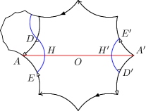
Figure 8.

For case of $4g+2$-cyclic symmetry we will pick two module.

(2) First polygon module of $4g+2$-cyclic case:

The hyperbolic surface of genus $g$ with $4g+2$-cyclic symmetry can be obtained by identifying opposite edges the regular hyperbolic 4g+2-polygon of angle sum $4\pi$. Below we denote this surface by $\Sigma^{2}_{g}$ and the polygon by $P_{2,g}$, often $P_{2}$ for short. Note all vertices in $P_{2}$ are alternatively identified to two points in $\Sigma^{2}_{g}$. Each angle of $P_{2}$ is $2\pi/(2g+1)$. We often view $P_{2}$ as a polygon contained either in $\Sigma^{2}_{g}$ or in the hyperbolic plane $\mathbb{H}^{2}$ .

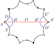
Figure 9.

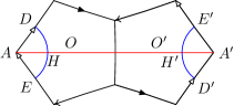
Figure 10.

(3) Dual fundamental region, the second polygon module of $4g+2$ case.

For regular hyperbolic $n$-gon $P_{i}\subset\mathbb{H}^{2}$, $i=1,2$, defined above, $D_{i}(P_{i})$ give a tessellation of $\mathbb{H}^{2}$, where $D_{i}$ is the deck transformation group such that $\mathbb{H}^{2}/D_{i}=\Sigma^{i}_{g}$. If two polygons in $D_{i}(P_{i})$ share one edge, connect their centers by the unique geodesic arc. The union of those arcs form a lattice, which provide a new tesselation $D_{i}(P_{i}^{*})$, where $P_{i}^{*}$ is also a fundamental region of $\Sigma_{g}^{i}$.

Figure 11.

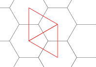
Figure 12.

One can check directly that

Proposition 2.

(1) $P_{1}^{*}$ is congruent to $P_{1}$, that is $P_{1}^{*}$ is also a regular hyperbolic 4g-polygon of angle sum $2\pi$. For each vertex $A$ of $P_{1}$, there is a unique $P_{1}^{*}$ centered at $A$.

(2) While $P_{2}^{*}$ is a union of two regular hyperbolic $2g+1$ polygons gluing along a pair of edges (see Figure 10), and each angle of the regular hyperbolic $2g+1$ polygon is $\pi/(2g+1)$. For each vertex $A$ of $P_{2}$, there is a unique $P_{2}^{*}$ such that one of its regular $(2g+1)$-gon centered at $A$.

Remark 1.

(1) Figure 12 and Figure 12 are the genus one counterparts of $P_{1}(P_{1}^{*})$ and $P_{2}(P_{2}^{*})$ respectively.

(2) $\Sigma^{2}_{g}$ is also obtained by identifying opposite edges the hyperbolic 4g-polygon $P^{*}_{2}$. Note all vertices in $P^{*}_{2}$ are identifed to one point in $\Sigma^{2}_{g}$. To see the $4g+2$-cyclic symmetry on $P_{2}^{*}$ directly, see [Wan91].

4.2. Candidates of systoles

In the regular polygons $P_{i}$, $i=1,2$, we call the geodesic that connects two opposite vertices a diameter. In $P_{2}^{*}$, call the geodesic connects two opposite vertices which is perpendicular to the common edge of two $2g+1$-regular polygons a diameter.

Now we will use one polygon $P$ below to present $P_{1}$, $P_{2}$ and $P_{2}^{*}$. where $O$ is the center of the whole $P$ when $P$ is either $P_{1}$ or $P_{2}$, and is the center of one of two $2g+1$ polygon when $P=P_{2}^{*}$, $AA^{\prime}$ is a chosen diameter of the polygon $P$. Let $D,E,D^{\prime},E^{\prime}$ be the mid-points of the corresponding edges neighboring the diameter. Then by symmetry it is not difficult to observe that the geodesic segments $DE$ and $E^{\prime}D^{\prime}$ form a closed geodesic $\gamma_{i}$ in $\Sigma_{g}^{i}$.

We are going to calculate the length of $\gamma_{i}$, $i=1,2$. Let $a$ be the angle between $OE$ and $OA$, and $b$ be the half of the angle at the vertex of the polygon. Then (see Figure 13).

(4.1) $$a=b=\frac{\pi}{4g}\,\text{for}\,{P_{1}};\,\,2a=b=\frac{2\pi}{4g+2}\,\text{for}\,P_{2};\,\,a=2b=\frac{2\pi}{4g+2},\text{for}\,P_{2}^{*}.$$

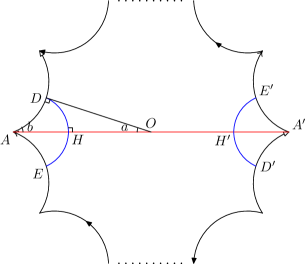
Figure 13.

Proposition 3.

In the polygons (see figure 13),

(1) $\cosh|OD|=\cos b/\sin a$,

(2) $\cosh|AD|=\cos a/\sin b$,

(3) $\cosh|OA|=\cot a\cot b$,

(4) $\sinh|DH|=\sqrt{\cos^{2}a-\sin^{2}b}$,

(5) $\cosh|DE|=2\left(\cos^{2}a-\sin^{2}b\right)+1$,

(6) $\cosh|AH|=\frac{\cos a}{\sin b\sqrt{\cos^{2}a+\cos^{2}b}}$,

(7) $\sinh|AH|=\cot b\sqrt{\frac{\cos^{2}a-\sin^{2}b}{\cos^{2}a+\cos^{2}b}}$.

In the surfaces the length of the geodesic $\gamma_{i}$ ($DEE^{\prime}D^{\prime}$) is $2\operatorname{arccosh}(1+\cos 2a+\cos 2b)$.

Proof.

In Figure 13, in the right-angle triangle $\triangle OAD$, $\angle ODA=\pi/2$, $\angle AOD=a$ and $\angle ODA=b$. Then by (3.4),

$$\cosh|OD|=\frac{\cos\angle OAD}{\sin\angle AOD}=\frac{\cos b}{\sin a},$$

and

$$\cosh|AD|=\frac{\cos\angle AOD}{\sin\angle DAO}=\frac{\cos a}{\sin b}.$$

By (3.2),

$$\cosh|OA|=\cosh|OD|\cosh|AD|=\cot a\cot b.$$

In the right-angled triangle $\triangle ADH$, $\angle DHA=\pi/2$, $\angle DAH=b$ and $\cosh|AD|=\cos a/\sin b$. Then by (3.3),

$$\sinh|DH| = \sinh|AD|\sin\angle DAH$$

$$= \sqrt{\left(\frac{\cos a}{\sin b}\right)^{2}-1}\sin b$$

$$= \sqrt{\cos^{2}a-\sin^{2}b}.$$

Therefore,

$$\cosh|DE| = 2\sinh^{2}|DH|+1$$

$$= 2\left(\cos^{2}a-\sin^{2}b\right)+1$$

$$= \cos 2a+\cos 2b+1.$$

Then $\cosh|DH|=\sqrt{\sinh^{2}|DH|+1}=\sqrt{\cos^{2}a+\cos^{2}b}$ and by (3.2),

$$\cosh|AH| = \cosh|AD|/\cosh|DH|$$

$$= \frac{\cos a}{\sin b\sqrt{\cos^{2}a+\cos^{2}b}}.$$

$$\sinh|AH| = \sqrt{\cosh^{2}|DH|-1}$$

$$= \cot b\sqrt{\frac{\cos^{2}a-\sin^{2}b}{\cos^{2}a+\cos^{2}b}}.$$

The length of the geodesic $\gamma_{i}$ ($DEE^{\prime}D^{\prime}$) is equal to $2|DE|$. Thus by (5) we have

(4.2) $$|\gamma_{i}|=2\operatorname{arccosh}(1+\cos 2a+\cos 2b).$$

∎

Let $2h_{i}$ be the length of $\gamma_{i}$, by plugging (4.1) into (4.2) we get

Corollary 3.

$$h_{1}=\operatorname{arccosh}(\cos\pi/2g+1)\,\text{and}\,h_{2}=\operatorname{arccosh}(1+\cos\frac{\pi}{2g+1}+\cos\frac{2\pi}{2g+1})$$

5. Injective radious $h_{i}$

5.1. Some reductions

Now we begin to prove $2h_{i}$ is the systole of the hyperbolic surface $\Sigma^{i}_{g}$, $i=1,2$. By definitions and Proposition 3, we have the following

Claim 1.

$B(x,h_{i})\to\Sigma^{i}_{g}$ is an embedding for each $x\in\Sigma_{g}^{i}$ implies that $\operatorname{sys}(\Sigma^{i}_{g})=2h_{i}$, $i=1,2$.

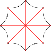
Figure 14.

We view $P_{i}$ as a polygon contained in $\Sigma^{i}_{g}$. There is an observation that every closed essential geodesic in $\Sigma_{g}^{i}$ must meet a diameter of $P_{i}$, since the diameters of $P_{i}$ cut $\Sigma_{g}^{i}$ into contractible pieces (see Figure 14). In particular each closed shortest geodesic meets a diameter of $P_{i}$. Note that all points in closed shortest geodesics have the same injective radious (see page [PAR06, p.178]).

Therefore we can reduce Claim 1 to the following:

Claim 2.

$B(x,h_{i})\to\Sigma^{i}_{g}$ is an embedding for each $x\in AA^{\prime}$ implies that $\operatorname{sys}(\Sigma^{i}_{g})=2h_{i}$, , $i=1,2$.

Let $H$, $H^{\prime}$ be the intersections of the diameter $AA^{\prime}$ and the geodesic segment $DE$ and $E^{\prime}D^{\prime}$ respectively, see Figure 13.

In each of the following two pictures Figure 15 and 16, the black polygon is $P_{i}$, and the green one is the dual polygon $P_{i}^{*}$ around the vertex $A$, where Figure 15 is for $i=1$ and Figure 16 is for $i=2$. By symmetry and Claim 2, we need only consider $x\in OA\subset P_{i}$. Note $OA=OH\cup HA$ and $A$ is the center of $P_{1}^{*}$ in Figure 15 and the center of one of the two $2g+1$ polygon of $P_{2}^{*}$. Moreover $P^{*}_{1}$ is a polygon congruent to $P_{1}$. We reduce Claim 2 to the following

Claim 3.

(1) $B(x,h_{1})\to\Sigma_{g}^{1}$ is an embedding for each $x\in OH\subset P_{1}$ implies that $\operatorname{sys}(\Sigma^{1}_{g})=2h_{1}$;

(2) $B(x,h_{2})\to\Sigma_{g}^{2}$ is an embedding for each $x\in OH\subset P_{2}$ and for each $x\in OH\subset P_{2}^{*}$ implies that $\operatorname{sys}(\Sigma^{i}_{g})=2h_{i}$

We remind the reader that in $P_{2}^{*}$, $O$ is the center of one of two $2g+1$ polygons as is defined in Section 4.2.

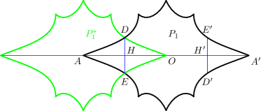
Figure 15.

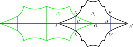
Figure 16.

5.2. Lift $B(x,h_{i})$ to the universal cover

Below for $B(x,h_{i})$ we assume that $x\in OH\subset P$.

Proposition 4.

For the polygon $P$,

(1) The distance between any vertex in the polygons and the segment $OH$ is bigger than $h_{i}$ for $P=P_{1},P_{2},P_{2}^{*}$.

(2) The distance between an edge and the diameter $AA^{\prime}$ is larger than $h_{i}$ except the nearest and second nearest edges for either $P=P_{1}$ and $g\geq 3$, or $P=P_{2}$ and $g\geq 2$, or $P=P_{1}^{*}$ and $g\geq 4$.

Proof.

(1) In Figure 17, $AA^{\prime}$ is a diameter of the polygon , $O$ is the center of either 4g-gon $P_{1}$, or (4g+2)-gon $P_{2}$, or the center of the $2g+1$-gon of $P_{2}^{*}$ containing $A$. $V$ is a vertex of the polygon $P_{1},P_{2}$ or the $2g+1$ polygon of $P_{2}^{*}$ containing $A$.

. Thus $|OV|=|OA|$. By Proposition 3 (3), $\cosh|OV|=\cot a\cot b$. $\alpha=2ka$, $k\in\mathbb{N}$. Distance between $AA^{\prime}$ and $V$ is realized by $|VR|$. By (3.3),

$$\sinh|VR| = \sinh|OV|\sin\alpha$$

$$= \sqrt{\cot^{2}a\cot^{2}b-1}\sin 2ka$$

$$\geq \sqrt{\cot^{2}a\cot^{2}b-1}\sin{2a}.$$

We use computer to compare $|VR|$ and $h_{i}$, finding that $|VR|\geq h_{i}$ if $P=P_{1},P_{2}$ or the $2g+1$ polygon of $P_{2}^{*}$ containing $A$. Vertices of the other $2g+1$ polygon of $P_{2}^{*}$ do not meet $B(x,h_{2})$ is a corollary of Proposition 4 (2).

Figure 17.

(2) In Figure 18, $AA^{\prime}$ is a diameter and $O$ is the center of $P_{1},P_{2}$ or the center of the $2g+1$ polygon of $P_{2}^{*}$ containing $A$. $E$ is the mid-point of an edge of the polygon $P_{1},P_{2}$ or the $2g+1$ polygon of $P_{2}^{*}$ containing $A$. $|OE|$ is the distance from the edge to $O$. By Proposition 3 (1), $\cosh|OE|=\cos b/\sin a$. $\beta=(2k+1)a$, $k\in\mathbb{N}$. Distance between $AA^{\prime}$ and the edge is realized by $|R_{1}R_{2}|$. By (3.7),

$$\cosh|R_{1}R_{2}| = \cosh|OE|\sin\beta$$

$$= \frac{\cos b\sin(2k+1)a}{\sin a}.$$

Then we compare $|R_{1}R_{2}|$ and $h_{i}$ by computer. We get: $|R_{1}R_{2}|<h_{i}$ when $k\leq 2$; $|R_{1}R_{2}|\geq h_{i}$ when $k\geq 3$, if $P=P_{1}$ and $g\geq 3$ or $P=P_{2}$ and $g\geq 2$ or $P=P_{2}^{*}$ and $g\geq 4$.

Figure 18.

∎

Proposition 5.

The upper half of a lift of $B(x,h_{i})$ in $\mathbb{H}^{2}$ doesn’t intersect any edges of the tessellation induced by the polygon other than edges $AB_{1},AB_{2},B_{1}C_{1}$ in Figure 19, if $P=P_{1}$ and $g\geq 4$; if $P=P_{2}$ and $g\geq 7$ or if $P=P_{2}^{*}$ and $g\geq 3$.

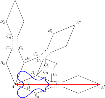
Figure 19.

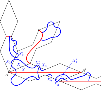
Figure 20.

This proposition characterizes the shape of $B(x,h_{i})$.

Proof.

By Proposition 4, $B(x,h_{i})$ may intersect $AB_{1}$ and $B_{1}C_{1}$ in their interior in all of the three models.

First, we calculate the distance between the segment $OH$ and $AB_{j}$ ($j=1,2,3$).

Lemma 1.

The distance between $OH$ and $AB_{j}$ ($j=1,2$) is smaller than $h_{i}$, while the distance between $OH$ and $AB_{3}$ is bigger than $h_{i}$, if $P=P_{1}$ and $g\geq 4$, if $P=P_{2}$ and $g\geq 7$, if $P=P_{2}^{*}$ and $g\geq 3$.

Proof.

We calculate this result by Figure 22. In this figure, $AA^{\prime}$ is a diameter and $AB_{j}$ is an edge. $x$ is a point on $AA^{\prime}$ between $H$ and $O$. Thus $\inf d(x,A)=|AH|$ for $x$ between $H$ and $O$. $\angle A=(2j-1)b$. Then the infimum distance $Rx$ between $x$ and $AB_{i}$ is

$$\inf_{x\in OH}\sinh|Rx| = \sin A\inf_{x\in OH}\sinh Ax\,\,\,\,(\text{by (\ref{for_tri_3})})$$

$$= (\sin(2j-1)b)\sinh|AH|$$

$$= (\sin(2j-1)b)\cot b\sqrt{\frac{\cos^{2}a-\sin^{2}b}{\cos^{2}a+\cos^{2}b}}\,\,\,\,(\text{by Prop. 3(2)})$$

by (3.3). Then we compare $\inf_{x\in OH}|Rx|$ and $h_{i}$ by computer programming. We get $\inf_{x\in OH}|Rx|\leq h_{i}$ for $j=1,2$ and $\inf_{x\in OH}|Rx|>h_{i}$ for $j=3$, if $P=P_{1}$ and $g\geq 4$; if $P=P_{2}$ and $g\geq 7$ or if $P=P_{2}^{*}$ and $g\geq 3$. Therefore, the lemma is proved. ∎

Lemma 1 is equivalent to say that $B(x,h_{i})$ may intersect $AB_{1}$ or $AB_{2}$, but won’t meet $AB_{3}$ or any other further edges whose one vertex is $A$.

Figure 21.

Figure 22.

Lemma 2.

$h_{i}$ is smaller than the distance between any two edges of the polygon that does not intersect.

Proof.

It is sufficient to calculate the distance between two nearest non-intersecting edges in a polygon. In Figure 22, $A,B$ are vertices of the polygon, $\angle A=\angle B=2b$. $AC$ and $BD$ are parts of edges of the polygon. $AB$ is an edge and thus $|AB|=2\operatorname{arccosh}\cos a/\sin b$ by Proposition 3. We calculate $|CD|$ by (3.11). Here

$$\cosh|CD| = \cosh|AB|\cdot\sin\angle A\sin\angle B-\cos\angle A\cos\angle B$$

$$= \left(\frac{2\cos^{2}a}{\sin^{2}b}-1\right)\sin^{2}2b-\cos^{2}2b.$$

We compare $|CD|$ with $h_{i}$, finding that $|CD|>h_{i}$ in all of the three models and obtain this conclusion.

∎

By Lemma 2, the $B(x,h_{i})$ doesn’t meet any edges in Figure 19 except $B_{1}C_{3}$, $C_{1}C_{2}$, $B_{1}C_{4}$, $B_{2}C_{6}$ and $AB_{j}$ ($j=1,2$).

Lemma 3.

$B(x,h_{i})$ doesn’t meet $B_{1}C_{4}$ and $B_{2}C_{6}$.

Proof.

The geodesic segment connecting the middle point of $AB_{0}$ and $AB_{1}$ is perpendicularly bisected by the diameter $AA^{\prime}$; the geodesic segment connecting the middle point of $B_{1}A$ and $B_{1}C_{4}$ is perpendicularly bisected by the diameter $B_{1}B_{1}^{\prime}$. The length of each segment is $h_{i}$ by Propostion 3. These two geodesic segments form a new geodesic segment which is perpendicular to both $AA^{\prime}$ and $B_{1}B_{1}^{\prime}$. Therefore, the distance between $AA^{\prime}$ and $B_{1}B_{1}^{\prime}$ is $h_{i}$. Thus $B(x,h_{i})$ doesn’t meet $B_{1}C_{4}$ since segment $B_{1}C_{4}$ is farthur to $AA^{\prime}$ than the line $B_{1}B_{1}^{\prime}$.

Similarly, distance between the diameters $B_{2}B_{2}^{\prime}$ and $AA^{\prime\prime}$ is not smaller than $h_{i}$. It implies that $B(x,h_{i})$ doesn’t meet $B_{2}C_{6}$.

We remind the reader that the two endpoints of the common perpendicular between $AA^{\prime}$ and $B_{1}B_{1}^{\prime}$ are $H$ and $H$’s deck transformation image on $B_{1}B_{1}^{\prime}$. This fact is useful in the proof of Corollary 1. ∎

Lemma 4.

$B(x,h_{i})$ doesn’t meet $B_{1}C_{3}$ and $C_{2}C_{1}$.

Proof.

First, we use Figure 24, which is a part of Figure 19, to calculate the distance between $B_{1}C_{3}$ and $AA^{\prime}$ in Figure 19. In Figure 24, $AB_{1}$ is an edge of the polygon and therfore its length is $2\operatorname{arccosh}\cos a/\sin b$. $\angle A=b$ while $\angle B_{1}=4b$. Then the distance between $AA^{\prime}$ and $B_{1}C_{3}$ (realized by $R_{1}R_{2}$ in the figure) is

$$\cosh|R_{1}R_{2}| = \sin\angle A\sin\angle B_{1}\cosh|AB_{1}|-\cos\angle A\cos\angle B_{1}$$

$$= \sin b\sin 4b\left(2\frac{\cos^{2}a}{\sin^{2}b}-1\right)-\cos b\cos 4b$$

by (3.11). By computer calculation, we know this distance is larger than $h_{i}$ in all of the three models.

Figure 23.

Figure 24.

Then, we use Figure 24, which is a part of Figure 19, to calculate the distance between $C_{1}C_{2}$ and $AA^{\prime}$ in Figure 19. In Figure 24, Since $C_{1}$ is a vertex of the regular polygon containing $A$, $|OC_{1}|$ is $\operatorname{arccosh}\cot a\cot b$. $\angle O=4a$ while $\angle C_{1}=3b$. Then the distance, realized by $R_{1}R_{2}$, between $AA^{\prime}$ and $C_{1}C_{2}$ is

$$\cosh|R_{1}R_{2}| = \sin\angle O\sin\angle C_{1}\cosh|OC_{1}|-\cos\angle A\cos\angle B_{1}$$

$$= \cot a\cot b\sin 4a\sin 3b-\cos 4a\cos 3b$$

by (3.11). We compare this distance with $h_{i}$, finding that $|R_{1}R_{2}|$ is larger than $h_{i}$ in all of the three models. ∎

∎

Now we have proved Proposition 5, that is $B(x,h_{i})$ in the universal cover $\mathbb{H}^{2}$ is shown as in Figure 19.

By projecting $B(x,h_{i})$ from the universal cover to $\Sigma_{g}^{i}$, we will get a picture of $B(x,h_{i})\subset P_{i}(P_{i}^{*})\subset\Sigma_{g}^{i}$ shown as in Figure 25

5.3. Back to $P$

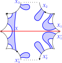
Figure 25.

Now it is sufficient to prove that any two components in Figure 25 does not intersect.

Two components in the polygon do not intersect each other if and only if the corresponding disks (lifts of $B(x,h_{i})$) in $\mathbb{H}^{2}$ does not intersect.

Lemma 5.

The interior of $X_{j}$ does not meet the diameter $AA^{\prime}$ for $j=1,2,3$

Proof.

$X_{1}$’s interior intersects $AA^{\prime}$ in Figure 25 if and only if in Figure 19, $B(x,h_{i})$’s interior intersects the diameter $B_{1}B_{1}^{\prime}$. But $d(AA^{\prime},B_{1}B_{1}^{\prime})=h_{i}$. Thus $X_{1}$’s interior does not intersect $AA^{\prime}$.

To prove $X_{2}$ in Figure 25 not meeting $AA^{\prime}$, it is sufficient to prove in Figure 19, the distance between $AA^{\prime}$ and $C_{2}C_{2}^{\prime}$ is larger than $h_{i}$.

In Figure 26, $d(AA^{\prime},C_{2}C_{2}^{\prime})$ is realized by segment $R_{5}R_{6}$. By using (3.7) in trirectangle with right angles $R_{5},R_{1},R_{2}$ and trirectangle with right angles $R_{6},R_{3},R_{4}$, we have $|R_{5}R_{6}|>|R_{3}R_{4}|+|R_{1}R_{2}|$. We calcuate $|R_{3}R_{4}|$ and $|R_{1}R_{2}|$ in the quadrilateral $R_{3}R_{4}B_{1}A$ and $R_{1}R_{2}C_{1}C_{2}$ respectively by (3.11). $\cosh|R_{3}R_{4}|=\cosh|AB_{1}|\sin\angle B_{1}AR_{3}\sin\angle AB_{1}R_{4}-\cos\angle B_{1}AR_{3}\cos\angle AB_{1}R_{4}$ and $\cosh|R_{1}R_{2}|=\cosh|C_{1}C_{2}|\sin\angle R_{1}C_{2}C_{1}\sin\angle C_{2}C_{1}R_{2}-\cos\angle R_{1}C_{2}C_{1}\cos\angle C_{2}C_{1}R_{2}$. Here $\angle B_{1}AR_{3}=\angle R_{1}C_{2}C_{1}=b$, $\angle AB_{1}R_{4}=\angle C_{2}C_{1}R_{2}=2b$, $|AB_{1}|=|C_{1}C_{2}|=2\operatorname{arccosh}\cos b/\sin a$. Therefore,

$$\cosh|R_{1}R_{2}|=\cosh|R_{3}R_{4}|=\left(2\frac{\cos^{2}a}{\sin^{2}b}-1\right)\sin 2b\sin b-\cos 2b\cos b.$$

We calculate $|R_{1}R_{2}|$ and $|R_{3}R_{4}|$ by computer, then compare $|R_{1}R_{2}|+|R_{3}R_{4}|$ with $h_{i}$ and get the following conclusion: $|R_{3}R_{4}|+|R_{1}R_{2}|>h_{i}$, and $X_{2}\cap AA^{\prime}=\emptyset$ in Figure 25 for all of the three models.

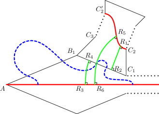
Figure 26.

$X_{3}$ in Figure 25 does not intersect $AA^{\prime}$ if and only if $B(x,h_{i})$ in Figure 19 does not intersect the diameter $C_{6}C_{7}$. $B(x,h_{i})$ in Figure 19 does not intersect the diameter $C_{6}C_{7}$, if $d(AA^{\prime},C_{6}C_{7})>h_{i}$.

We use Figure 27 to calculate $d(AA^{\prime},C_{6}C_{7})$. Figure 27 is a part of Figure 19. $O^{\prime}$ is the center of the regular polygon it is in. In the quadrilateral $AO^{\prime}R_{2}R_{1}$, $\angle A=4b,\angle O^{\prime}=4a$, $|O^{\prime}A|=\operatorname{arccosh}\cot a\cot b$ by Proposition 3. Then by (3.11),

$$\cosh|R_{1}R_{2}| =\cosh|AO^{\prime}|\sin\angle A\sin\O^{\prime}-\cos A\cos O^{\prime}$$

(5.1) $$=\cot a\cot b\sin 4a\sin 4b-\cos 4a\cos 4b.$$

By the help of the computer, we compare $|R_{1}R_{2}|$ and $h_{i}$, finding that $|R_{1}R_{2}|$ is larger than $h_{i}$ for all of the three models.

Figure 27.

∎

Figure 28.

Lemma 6.

In Figure 25, $X_{1},X_{2},X_{3}$ does not intersect $X$.

Proof.

(1) The distance between the polygon’s center and an edge is $\cos b/\sin a$ by Proposition 3. Then we compare it with $h_{i}$ by computer and the conclusion follows. For $g\geq 4$, distance between the polygon’s center and edges are bigger than $h_{i}$. If $X$ intersects $X_{1}$ or $X_{2}$, there are two radii of $B(x,h_{i})$ that intersect. It imples that the distance between two opposite edges is smaller or equal to $2h_{i}$, which is impossible. (See Figure 28. )

(2) $X\cap X_{3}=\emptyset$ in Figure 25 is equivalent to in Figure 19, the distance between $x$ on $AA^{\prime}$ and its deck transformation image on $C_{6}C_{7}$ is larger than $2h_{i}$. (See Figure 27) Now we prove this distance is larger than $2h_{i}$ by the formulae of the quadrilateral:

$x$ is a point moving on the diameter $AA^{\prime}$ between $H$ and $O$. $x^{\prime}$ is its deck transformation image. $x^{\prime}$ moves as $x$ moves. We calculate $\inf_{x\in HO}d(x,x^{\prime})$ and compare it with $2h_{i}$.

In Figure 27, we have obtained $|R_{1}R_{2}|$ in (5.1). Then in the quadrilateral $R_{1}R_{2}x^{\prime}x$, by (3.10),

$$\cosh|xx^{\prime}|=\cosh|R_{1}R_{2}|\cosh|R_{1}x|\cosh|R_{2}x^{\prime}|-\sinh|R_{1}x|\sinh|R_{2}x^{\prime}|.$$

Assume $|Ax|=t$, then $|R_{1}x|=|AR_{1}|-t$ and $|R_{2}x^{\prime}|=|R_{2}C_{6}|+t$. Here $|C_{6}x^{\prime}|=|Ax|=t$. $|AH|\leq t\leq|AO|$. Here $H$ is the intersecting point of the diameter and the geodesic connecting the mid-point of $AB_{0}$ and $AB_{1}$.

Then we denote $\cosh|xx^{\prime}|$ to be $f(t)$.

$$f(t)=\cosh|R_{1}R_{2}|\cosh(|AR_{1}|-t)\cosh(|C_{6}R_{2}|+t)-\sinh(|AR_{1}|-t)\sinh(|C_{6}R_{2}|+t).$$

Thus

$$f^{\prime}(t) = \cosh|R_{1}R_{2}|(-\sinh(|AR_{1}|-t)\cosh(|C_{6}R_{2}|+t)+\cosh(|AR_{1}|-t)\sinh(|C_{6}R_{2}|+t))-$$

$$(-\cosh(|AR_{1}|-t)\sinh(|C_{6}R_{2}|+t)+\sinh(|AR_{1}|-t)\cosh(|C_{6}R_{2}|+t))$$

$$= (\cosh|R_{1}R_{2}|-1)\sinh(2t-|AR_{1}|+|C_{6}R_{2}|).$$

Therefore, the minimum of $f(t)$ is obtained when $t=(|AR_{1}|-|C_{6}R_{2}|)/2$. At this point, $|R_{1}x|=|R_{2}x^{\prime}|=(|AR_{1}|+|C_{6}R_{2}|)/2$ and thus quadrilateral $xx^{\prime}R_{2}R_{1}$ is a quadrilateral with $\angle R_{1}=\angle R_{2}=\pi/2$, $\angle x=\angle x^{\prime}$. Moreover, $|Ax|+|O^{\prime}x^{\prime}|=|AO|$. ($|O^{\prime}x^{\prime}|=|O^{\prime}C_{6}|-|C_{6}x^{\prime}|=|AO|-|Ax|$. )

To prove $|xx^{\prime}|>2h_{i}$, we construct a quadrilateral $R_{1}R_{2}S_{2}S_{1}$.(See Figure 29) In the quadrilateral $R_{1}R_{2}O^{\prime}A$, $\angle A=4b$ and $\angle O^{\prime}=4a$. Without loss of generality, we assume $b\geq a$. $S_{1}\in AR_{1}$, $S_{2}\in O^{\prime}R_{2}$, satisfying $\angle S_{1}S_{2}R_{2}=\angle S_{2}S_{1}R_{1}=4b$. (We remark that when $a=b$, $S_{1}=A$ and $S_{2}=O^{\prime}$). Such $S_{1}$ and $S_{2}$ exist on the segment $R_{1}A$ and $R_{2}O^{\prime}$ respectively instead of on the extended lines of $R_{1}A$ and $R_{2}O^{\prime}$ because otherwise we’ll get a quadrilateral with sum of interior angles bigger than $2\pi$ or a triangle with sum of interior angles bigger than $\pi$, which is impossible.

Figure 29.

Then we pick up two points $y$, $y^{\prime}$ on $R_{1}S_{1}$ and $R_{2}S_{2}$ respectively, satisfying $|S_{1}y|=|S_{2}y^{\prime}|=|AO|/2$. Then $|R_{1}x|\geq|R_{1}y|$ and $|R_{2}x^{\prime}|\geq|R_{2}y^{\prime}|$ by the following argument: We have $|R_{1}A|\geq|R_{1}S_{1}|$, $|R_{2}O^{\prime}|\geq|R_{2}S_{2}|$ and $|Ax|+|O^{\prime}x^{\prime}|=|AO|$. Without loss of generality, we assume $|Ax|\leq|AO|/2\leq|O^{\prime}x^{\prime}|$. Then $|R_{1}y|=|R_{1}S_{1}|-|S_{1}y|=|R_{1}S_{1}|-|AO|/2\leq|R_{1}A|-|Ax|=|R_{1}x|$. Then $|R_{2}y^{\prime}|\leq|R_{2}x^{\prime}|$ follows from $|R_{1}x|=|R_{2}x^{\prime}|$ and $|R_{1}y|=|R_{2}y^{\prime}|$. This result means $|xx^{\prime}|\geq|yy^{\prime}|$ by (3.11).

To prove $|xx^{\prime}|\geq 2h_{i}$, it is sufficient to prove $|yy^{\prime}|\geq 2h_{i}$. Now we calculate $|yy^{\prime}|$ and compare it with $2h_{i}$. By the symmetry of the quadrilaterals $R_{1}R_{2}y^{\prime}y$, $R_{1}R_{2}x^{\prime}x$ and $R_{1}R_{2}S_{2}S_{1}$, the segment $R_{0}S_{0}$ divides each of these quadrilaterals into two equal trirectangles, namely $R_{0}R_{1}yy_{0}$ and $R_{0}R_{2}y^{\prime}y_{0}$; $R_{0}R_{1}xx_{0}$ and $R_{0}R_{2}x^{\prime}x_{0}$; $R_{0}R_{1}S_{1}S_{0}$ and $R_{0}R_{2}S_{2}S_{0}$. Here $R_{0}$, $y_{0}$, $x_{0}$ and $S_{0}$ are the middle points of $R_{1}R_{2}$, $yy^{\prime}$, $xx^{\prime}$ and $S_{1}S_{2}$ respectively. Thus $|yy^{\prime}|\geq 2h_{i}$ is equivalent to $|yy_{0}|\geq h_{i}$. Now we calculate $|yy_{0}|$.

By our construction, in the trirectangle $R_{1}R_{0}S_{0}S_{1}$, $\angle R_{0}=\angle R_{1}=\angle S_{0}=\pi/2$, $\angle S_{1}=4b$. $|R_{1}R_{2}|$ is obtained in (5.1). Then we get $\coth\frac{|R_{1}R_{2}|}{2}$:

$$\cosh\frac{|R_{1}R_{2}|}{2} =\sqrt{\frac{\cosh|R_{1}R_{2}|+1}{2}}$$

$$=\sqrt{\frac{\cot a\cot b\sin 4a\sin 4b-\cos 4a\cos 4b+1}{2}},$$

$$\sinh\frac{|R_{1}R_{2}|}{2} =\sqrt{\frac{\cosh|R_{1}R_{2}|-1}{2}}$$

$$=\sqrt{\frac{\cot a\cot b\sin 4a\sin 4b-\cos 4a\cos 4b-1}{2}},$$

$$\coth\frac{|R_{1}R_{2}|}{2} =\cosh\frac{|R_{1}R_{2}|}{2}/\sinh\frac{|R_{1}R_{2}|}{2}$$

$$=\sqrt{\frac{\cot a\cot b\sin 4a\sin 4b-\cos 4a\cos 4b+1}{\cot a\cot b\sin 4a\sin 4b-\cos 4a\cos 4b-1}}.$$

Then by (3.9), we obtain $|R_{1}S_{1}|$:

$$\sinh|R_{1}S_{1}| =\coth\frac{|R_{1}R_{2}|}{2}\cot\angle S_{0}S_{1}R_{1}$$

$$=\coth\frac{|R_{1}R_{2}|}{2}\cot 4b$$

Then we obtain $|R_{1}y|$:

$$\cosh|R_{1}y| =\cosh(|R_{1}S_{1}|-|S_{1}y|)$$

$$=\cosh(|R_{1}S_{1}|-|AO|/2)$$

$$=\cosh|R_{1}S_{1}|\cosh\frac{|AO|}{2}-\sinh|R_{1}S_{1}|\sinh\frac{|AO|}{2}$$

Here $|AO|=\operatorname{arccosh}(\cot a\cot b)$.

Finally, we get $|yy_{0}|$ by (3.8):

$$\sinh|yy_{0}|=\sinh|R_{0}R_{1}|\cosh|R_{1}y|$$

.

By computer programming, we compare $yy_{0}$ and $h_{i}$, finding that $yy_{0}>h_{i}$ and therefore $X\cap X_{3}=\emptyset$ in Figure 27.

We remark that the proof above also proves $X_{1}\cap X_{2}=\emptyset$, see Figure 27.

∎

Lemma 7.

In Figure 25, $X_{1},X_{2},X_{3}$ do not intersect each other when $g\geq 4$.

Proof.

The proof of $X\cap X_{3}=\emptyset$ in Lemma 6 also proves $X_{1}\cap X_{2}=\emptyset$. Below we prove (1) $X_{2}\cap X_{3}=\emptyset$ (2) $X_{1}\cap X_{3}=\emptyset$.

In $P_{1}$ model, we pick the diameter perpendicular to $AA^{\prime}$ (denoted $BB^{\prime}$). Now we prove that $X_{1},X_{2},X_{3}$ cannot meet $BB^{\prime}$, and therefore $X_{1}\cap X_{3}=\emptyset$ and $X_{2}\cap X_{3}=\emptyset$. (See Figure 31. )

Figure 30.

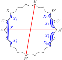
Figure 31.

The proof of $X_{i}\cap BB^{\prime}=\emptyset$ are exactly the same for $i=1,2,3$. Without loss of generality, we prove that $X_{3}\cap BB^{\prime}=\emptyset$. , In Figure 31, we denote the edge that meets $X_{3}$ to be $CD$. Since $g\geq 4$, the edge $CD$ is not the nearest and the second nearest edge to the diameter $BB^{\prime}$, by Proposition 4 (2), $d(BB^{\prime},CD)>h_{i}$. On the other hand, the center $x^{\prime}$ of the $B(x^{\prime},h_{i})$ containing $X_{3}$ is outside the polygon in Figure 31. Therefore, $\forall x_{3}\in X_{3}$, $d(x_{3},CD)\leq h_{i}$. Thus $X_{3}\cap BB^{\prime}=\emptyset$.

In $P_{2}$ model, let $BB^{\prime}$ be one of the diameters whose angle with $AA^{\prime}$ is the biggest, see Figure 31. Since $g\geq 4$ and $P_{2}$ is 4g+2 gon, we still can apply Proposition 4 (2) to prove $X_{i}\cap BB^{\prime}=\emptyset$ for $i=1,2,3$ exactly as $P_{1}$ case, and then $X_{1}\cap X_{3}=\emptyset$, $X_{2}\cap X_{3}=\emptyset$.

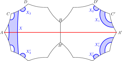
Figure 32.

In $P_{2}^{*}$ model, we let $BB^{\prime}$ be the edge seperate the two $2g+1$ polygons and the edge that meets $X_{3}$ be $CD$ (See Figure 32) Since $g\geq 4$, $2g+1\geq 9$, the edge $CD$ and the edge $BB^{\prime}$ are disjoint. Then by Lemma 2, $d(BB^{\prime},CD)>h_{i}$. On the other hand, the center $x^{\prime}$ of the $B(x^{\prime},h_{i})$ that corresponds to $X_{3}$ is outside the polygon in Figure 32. Therefore, $\forall x_{3}\in X_{3}$, $d(x_{3},CD)\leq h_{i}$. Thus $X_{3}\cap BB^{\prime}=\emptyset$.

By exactly the same proof, we have $X_{i}\cap BB^{\prime}=\emptyset$ for $i=1,2$. So that $X_{1}\cap X_{3}=\emptyset$ and $X_{2}\cap X_{3}=\emptyset.$

We have proved the theorem.

∎

Now we begin to prove Corollary 1.

Corollary 1.

In $\Sigma_{g}^{1}$, there are $2g$ closed geodesics having length $\operatorname{sys}(\Sigma_{g}^{1})$ and in $\Sigma_{g}^{2}$, there are $2g+1$ closed geodesics having length $\operatorname{sys}(\Sigma_{g}^{2})$.

Proof.

By the proof of Lemma 5, Lemma 6 and Lemma 7, each pair of components in Figure 25 does not intersect except $X_{1}$ and $X_{1}^{\prime}$. $X_{1}$ and $X_{1}^{\prime}$ may be tangent to each other. For a fixed $x$ (center of the ball $B(x,h_{i})$) on $OH$, the number of points in $\partial X_{1}\cap\partial X_{1}^{\prime}$ is $0$ or $1$ by the convexity of balls in hyperbolic plane. The only thing to show is $\partial X_{1}\cap\partial X_{1}^{\prime}\neq\emptyset$ if and only if $x$ is the point $H$.

This fact is straight forward by the proof of Lemma 3. In that proof, the common perpendicular between $AA^{\prime}$ and $B_{1}B_{1}^{\prime}$ in Figure 19 is the segment connecting $H$ and $H$’s deck transformation image on $B_{1}B_{1}^{\prime}$. Besides, $d(AA^{\prime},B_{1}B_{1}^{\prime})=h_{i}$. Therefore $d(x,B_{1}B_{1}^{\prime})\geq h_{i}$, $\forall x\in OH$. The equality holds if and only if $x=H$. It proves that in Figure 25, $X_{1}\cap AA^{\prime}=\{H^{\prime}\}$ and $X_{1}^{\prime}\cap AA^{\prime}=\{H^{\prime}\}$ if and only if $x=H$. (Here $H^{\prime}$ is the intersecting point of $E^{\prime}D^{\prime}$ and $AA^{\prime}$ in Figure 13. )

Then it proves that $\gamma_{i}$ ($DEE^{\prime}D^{\prime}$ in Figure 13) is the unique systole that intersects $OH$ in all of the three models. By Claim 3, $\gamma_{i}$ is the unique systole that intersects $OA$ in $P_{1}$ and $P_{2}$. By the invariance of $\gamma_{i}$ under the $\pi$-rotation of $P_{1}$ and $P_{2}$, $\gamma_{i}$ is the unique systole that intersects $AA^{\prime}$ in $P_{1}$ and $P_{2}$. This is equivalent to that given a diameter of $P_{1}$ or $P_{2}$, there is a unique systole intersects the diameter. Therefore by counting the number of diameters of $P_{1}$ and $P_{2}$, the Corollary holds.

∎

6. Appendix

In this Section, we give the source code and figure for the comparison between $|CD|$ and $h_{i}$ in Lemma 2. The code is written in MATLAB. The codes for other comparisons are similar.

⬇

1

2%P_1 model

3a = [eps:eps:pi/8];

4b = a;

5%P_2 model

6%a = [eps:eps:pi/10];

7%b = 2*a;

8%P_2^* model

9%a = [eps:eps:pi/5];

10%b = 0.5*a;

11

12chdst = (2*(cos(a)./sin(b)).^2-1).*(sin(2*b)).^2-(cos(2*b)).^2;

13

14chh = 1 + cos(2*a) + cos(2*b);

15%shh = sqrt(chh.^2-1);

16f = chdst - chh;

17plot(a,f);

Figure 33 shows the result of the comparison in $P_{1}$ model. In Figure 33, the horizontal axis is the variable $a$, while the vertical axis is $\cosh|CD|-\cosh h_{i}$ (depends on $a$).

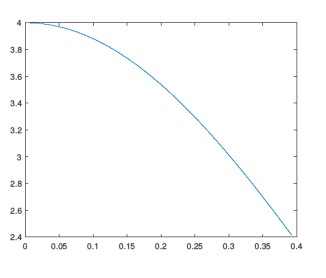
Figure 33.

References

- [Bav92] Christophe Bavard. La systole des surfaces hyperelliptiques. Prepubl. Ec. Norm. Sup. Lyon, 71, 1992.
- [BS94] Peter Buser and Peter Sarnak. On the period matrix of a riemann surface of large genus (with an appendix by jh conway and nja sloane). Inventiones mathematicae, 117(1):27–56, 1994.
- [Bus10] Peter Buser. Geometry and spectra of compact Riemann surfaces. Springer Science & Business Media, 2010.
- [GWWZ15] Yu Guo, Chao Wang, Shicheng Wang, and Yimu Zhang. Embedding periodic maps on surfaces into those on . Chinese Annals of Mathematics, Series B, 36(2):161–180, March 2015.
- [Hu] A. Hurwitz, Über algebraische Gebilde mit eindeutigen Transformationen in sich, Math. Ann. 41 (1893), 403-442
- [Jen84] Felix Jenni. Über den ersten eigenwert des laplace-operators auf ausgewählten beispielen kompakter riemannscher flächen. Commentarii Mathematici Helvetici, 59(1):193–203, 1984.
- [KSV07] Mikhail G Katz, Mary Schaps, Uzi Vishne, Logarithmic growth of systole of arithmetic riemann surfaces along congruence subgroups. Journal of Differential Geometry, 76(3):399–422, 2007.
- [Kul97] Ravi S Kulkarni. Riemann surfaces admitting large automorphism groups. Extremal Riemann surfaces (San Francisco, CA, 1995), 201:63–79, 1997.
- [Par14] Hugo Parlier. Simple closed geodesics and the study of teichmüller spaces. Handbook of Teichmüller Theory, Volume IV, pages 113–134, 2014.
- [PAR06] Peter Petersen, S Axler, and KA Ribet. Riemannian geometry, volume 171. Springer, 2006.
- [Pet18] Bram Petri. Hyperbolic surfaces with long systoles that form a pants decomposition. Proceedings of the American Mathematical Society, 146(3):1069–1081, 2018.
- [PW15] Bram Petri and Alexander Walker. Graphs of large girth and surfaces of large systole. arXiv preprint arXiv:1512.06839, 2015.
- [Sch93] P Schmutz. Reimann surfaces with shortest geodesic of maximal length. Geometric & Functional Analysis GAFA, 3(6):564–631, 1993.
- [Wan91] Shicheng Wang. Maximum orders of periodic maps on closed surfaces. Topology and its Applications, 41(3):255–262, 1991.
- [Wim95] A. Wiman, Uber die hyperelliptischen Kurven und diejenigen vom Geschlecht p=3, welche eindeutige Transformationen in sich zulassen, Bihang Till. Kongl. Svenska Vetenskaps-Akademiens Handlingar 21 (1) 1895.