The unitarity expansion for light nuclei

Abstract

I is argued here that (at least light) nuclei may reside in a sweet spot: bound weakly enough to be insensitive to the details of the interaction, but dense enough to be insensitive to the exact values of the large two-body scattering lengths as well. In this scenario, a systematic expansion of nuclear observables around the unitarity limit converges. In particular, in this scheme the nuclear force is constructed such that the gross features of states in the nuclear chart are determined by a very simple leading-order interaction, whereas—much like the fine structure of atomic spectra—observables are moved to their physical values by small perturbative corrections. Explicit evidence in favor of this conjecture is shown for the binding energies of three and four nucleons.

1 Introduction

Ever since the effective range expansion (ERE) was developed as a theory to parameterize the low-energy two-nucleon system [1, 2, 3, 4] it has been known that the nucleon-nucleon ($N\!N$) scattering lengths, $a_{t}\simeq 5.4\leavevmode\nobreak\ \mathrm{fm}$ and $a_{s}\simeq{-}23.7\leavevmode\nobreak\ \mathrm{fm}$ in the ${}^{3}S_{1}$ and ${}^{1}S_{0}$ channels, respectively, are large compared to the typical range of the nuclear interaction, $R\sim M_{\pi}^{-1}\simeq 1.4\leavevmode\nobreak\ \mathrm{fm}$, set by the inverse pion mass. Considering quantum chromodynamics (QCD) as the underlying theory of the strong interaction, this particular feature of the low-energy two-nucleon ($2N$) system can be understood as an accidental “fine tuning” of the QCD parameters [5, 6, 7, 8, 9] (the quark masses) to be close to a critical point where the scattering lengths are infinite, the so-called “unitarity (or unitary) limit.”

This curiosity of nature has profound consequences for the theoretical description of few-nucleon systems at low energies, placing them in the same universality class as other systems governed by large scattering lengths, such as cold atomic gases, where the scattering length can be tuned via Feshbach resonances [10], or certain mesons which can be interpreted as hadronic molecules [11]. Most notably, the triton is understood to be the single remaining bound state out of an infinite tower of Efimov states [12] that exists in the exact unitarity limit [13, 14, 15]. Recently, it was shown in a model-independent way that a virtual state in the three-nucleon ($3N$) system, known to exist for a long time [16, 17], is as an S-matrix pole that would be an excited Efimov state if nature were just a bit closer to the unitarity limit [18], confirming a relation previously observed in a separable potential model [19].

Following Ref. [20] it is argued here that nature is indeed close enough to unitarity such that it is possible to quantitatively describe the spectra of—at least light, and possible also heavier—nuclei by a perturbative expansion around the limit of infinite two-body scattering lengths. At leading order (LO) this yields an interaction which is parameter free in the $2N$ sector and determined by a single three-body parameter, adjusted to keep the triton binding energy fixed at its experimental value. This remarkably simple theory is shown to capture the gross features of nuclei up to ${}^{4}\mathrm{He}$, while corrections such as the actual finite values of the $2N$ scattering lengths and electromagnetic effects are accounted for in perturbation theory.

Quantitatively, this “unitarity expansion” is constructed as a variant of pionless effective field theory (pionless EFT). This theory, most recently reviewed in Ref. [21], describes low-energy nuclear systems in a model-independent way, guided only by the symmetries of QCD and the universal physics of systems governed by a large scattering length. As such, it is ideally suited to set up the unitarity expansion with a minimal set of assumptions. An important aspect of each EFT is the organizational principle called “power counting,” which attributes the various terms to different orders in a systematic expansion. In the standard pionless theory, the expansion parameter is given by a typical low-momentum scale $Q$ divided by the high scale $R^{{-}1}\sim M_{\pi}$. The unitarity expansion is obtained by assuming that $Q\sim Q_{A}=\sqrt{2M_{N}B_{A}/A}$, placing nuclei in a “sweet spot” $1/a_{s,t}<Q_{A}<1/R$, where a combined expansion in $Q_{A}R$ and $1/(Q_{A}a_{s,t})$ converges.

In the following, the formalism is discussed in more detail by describing its application to calculate systems of up to four nucleons. Readers not interested in more technical details are invited to skip ahead to Sec. 3, which presents the main results and provides a broader perspective that places the unitarity expansion in line with other recent results suggesting a fascinating simplification of nuclear physics.

2 Formalism

Following the notation of Refs. [22, 20], pionless EFT is defined in terms of a Lagrange density

$$\mathcal{L}=N^{\dagger}\left(\mathrm{i}{\cal D}_{0}+\frac{\boldsymbol{\cal D}^{2}}{2M_{N}}\right)N\hbox{}+\sum\nolimits_{\mathbf{i}}C_{0,\mathbf{i}}\left(N^{T}P_{\mathbf{i}}N\right)^{\dagger}\left(N^{T}P_{\mathbf{i}}N\right)+D_{0}\left(N^{\dagger}N\right)^{3}+\cdots\,,$$ (3)

involving nonrelativistic nucleon isospin doublets $N=(p\;n)^{T}$ as well as photon fields $A_{\mu}$ which are coupled to the nucleons via the covariant derivative $\mathcal{D}_{\mu}=\partial_{\mu}+\mathrm{i}eA_{\mu}(1+\tau_{3})/2$, where $e$ is the proton charge and $\tau_{a}$ is used to label isospin Pauli matrices. Besides these electromagnetic interactions, of which only the static Coulomb potential is relevant to the order considered here, the theory involves only contact (zero range) interactions proportional to “low-energy constants” (LECs), such as the $C_{0,\mathbf{i}}$, $D_{0}$ shown in Eq. (3), plus other contributions (involving an increasing number of derivatives acting on the nucleon fields) contained in the ellipses. The $P_{\mathbf{i}}$ denote projectors onto the $N\!N$ $S$ waves, $\mathbf{i}={}^{1}S_{0},{}^{3}S_{1}$, corresponding to the short-hand labels used above for the singlet and triplet scattering lengths.

Leading-order (LO) terms are summed up to all orders in a nonperturbative treatment to which higher-order corrections are added in perturbation theory. This procedure implies that the LECs of all operators are split into different orders, e.g., $C_{0,\mathbf{i}}=C_{0,\mathbf{i}}^{(0)}+C_{0,\mathbf{i}}^{(1)}+\cdots$. Typically, only the leading term in this expansion introduces a new parameter whereas the higher-order contributions are merely used to maintain lower-order renormalization conditions as additional corrections are included. The unitarity expansion departs from this scheme by moving the introduction of two-body parameters from $C_{0,\mathbf{i}}^{(0)}$ to $C_{0,\mathbf{i}}^{(1)}$.

The LO calculation can be carried out in closed form by solving the Lippmann-Schwinger equation for a separable potentials $V_{2,\mathbf{i}}^{(0)}=C_{0,\mathbf{i}}^{(0)}|g\rangle\langle g|$, where $\langle p|g\rangle=g(p^{2})=\exp({-}p^{2}/\Lambda^{2})$ with a cutoff scale $\Lambda$ is a Gaussian regulator and $p$ is the $N\!N$ center-of-mass momentum. This is shown diagrammatically in Fig. 1. Some results discussed in Sec. 3 are obtained using a slightly different implementation, employing so-called “dibaryon” fields to describe the two-body sector and using a sharp momentum cutoff, which is essentially equivalent to choosing $\langle p|g\rangle$ to be a step function. This approach, deriving two- and three-body equations directly from Feynman diagrams has been discussed in detail in Refs. [22, 23], so that here only the potential formalism with Gaussian regulator is considered.

Figure 1: Diagrammatic version of the Lippmann-Schwinger equation for the two-nucleon T-matrix at LO, depicted by the circled zero. The solid lines represent nucleon fields, whereas the dot represents a contact interaction $C_{0,\mathbf{i}}^{(0)}$.

Starting from $t_{\mathbf{i}}^{(0)}=V_{2,\mathbf{i}}^{(0)}+V_{2,\mathbf{i}}^{(0)}G_{0}t_{\mathbf{i}}^{(0)}$, where $G_{0}$ is the free two-body Green’s function, the separable form of the interaction makes it possible to directly write down the solution as

$$t_{\mathbf{i}}^{(0)}(z;\mathbf{k},\mathbf{k}^{\prime})=\langle\mathbf{k}|t_{\mathbf{i}}^{(0)}|\mathbf{k}^{\prime}\rangle=g(k^{2})\tau_{\mathbf{i}}(z)g(k^{\prime 2})\ \ \text{,}\ \ \tau_{\mathbf{i}}(z)=\left[1/{C_{0,\mathbf{i}}^{(0)}}-\langle g|G_{0}|g\rangle\right]^{-1}\,,$$ (4)

where $z$ denotes the energy. $C_{0,\mathbf{i}}^{(0)}$ can now be determined by matching this T-matrix to the effective range expansion at the on-shell point, $\mathbf{k}=\mathbf{k}^{\prime}$ and $E=k^{2}/M_{N}$. The unitarity limit (infinite scattering length, $1/a_{\mathbf{i}}=0$) is reproduced by setting $C_{0,\mathbf{i}}^{(0)}=\frac{{-}2\pi^{2}}{M_{N}\Lambda}\theta^{-1}$, where $\theta=1/\sqrt{2\pi}$ for the Gaussian regulator used here. This means that the $C_{0,\mathbf{i}}^{(0)}$ do not introduce any physical parameters. At NLO, the correction to the T-matrix is

$$t_{\mathbf{i}}^{(1)}=V_{2,\mathbf{i}}^{(1)}+V_{2,\mathbf{i}}^{(1)}G_{0}t_{\mathbf{i}}^{(0)}+t_{\mathbf{i}}^{(0)}G_{0}V_{2,\mathbf{i}}^{(1)}+t_{\mathbf{i}}^{(0)}G_{0}V_{2,\mathbf{i}}^{(1)}G_{0}t_{\mathbf{i}}^{(0)}\,,$$ (5)

i.e., the sum of all possible terms linear in $V_{2,\mathbf{i}}^{(1)}$. The overall NLO T-matrices $t_{\mathbf{i}}^{(0)}+t_{\mathbf{i}}^{(1)}$ should reproduce the physical values of the $N\!N$ S-wave scattering lengths, which leads to $C_{0,\mathbf{i}}^{(1)}=\frac{M_{N}}{4\pi a_{\mathbf{i}}}C_{0,\mathbf{i}}^{(0)2}$. Note that instead of using Eq. (5) it is possible to conveniently obtain $t_{\mathbf{i}}^{(1)}$ as well as higher-order corrections by solving integral equations similar to the one defining $t_{\mathbf{i}}^{(0)}$. Details about this procedure can be found in Refs. [24, 23].

With the two-body LECs determined, it is possible to proceed with calculations for three and four nucleons. In the following the unified Faddeev + Faddeev-Yakubovsky (F+FY) framework that was used to obtain the four-nucleon results presented in Ref. [20]. The approach follows Refs. [25, 26, 27, 28] (which, in turn, are based on the work of Kamada and Glöckle [29]) but uses an independently developed numerical implementation. Since a fully comprehensive description of the method is beyond the scope of this work, emphasis is put here primarily on details regarding the perturbative treatment of NLO contributions.

Three nucleons

It is a distinct feature of pionless EFT that a three-nucleon interaction (3NI) enters at LO in the power counting, while naïvely it would be expected to contribute only much later. This promotion of the 3NI is a direct consequence of the unnaturally large $N\!N$ S-wave scattering length, leading to the triton as an effective Efimov state [13, 14, 15]. In the separable potential formalism the LO 3NI can be implemented as

$$V_{3}^{(0)}=D_{0}^{(0)}\,|{}^{3}\mathrm{H}\rangle|\xi\rangle\langle\xi|\langle{}^{3}\mathrm{H}|\,,$$ (6)

where $|{}^{3}\mathrm{H}\rangle$ projects onto a $J=T=\nicefrac{{1}}{{2}}$ three-nucleon state and the regulator is now defined, for Jacobi momenta $\mathbf{u}_{1}=\frac{1}{2}(\mathbf{k}_{1}-\mathbf{k}_{2})$ and $\mathbf{u}_{2}=\frac{2}{3}[\mathbf{k}_{3}-\frac{1}{2}(\mathbf{k}_{1}+\mathbf{k}_{2})]$, as $\langle\mathbf{u}_{1}\mathbf{u}_{2}|\xi\rangle=g\big{(}u_{1}^{2}+\frac{3}{4}u_{2}^{2}\big{)}$. The $\mathbf{k}_{i}$ label the individual nucleon momenta. The NLO correction $V_{3}^{(1)}$ has the same form as Eq. (6), but involves the LEC $D_{0}^{(1)}$.

The Faddeev equations in an abstract operator notation take the form [eq:Faddeev] —ψ⟩ &= G_0 t^(0) P —ψ⟩ + G_0 t^(0) —ψ_3⟩  ,
—ψ_3⟩ = G_0 t_3^(0) (1+P) —ψ⟩  , where $|\psi\rangle=|\psi_{(12)3}\rangle$ is one of the (equivalent) two-body Faddeev components and $|\psi_{3}\rangle$ is defined in terms of the three-body interaction $V_{3}$ [27]. $G_{0}$ now denotes the free three-body Green’s function and $P=P_{12}P_{23}+P_{13}P_{23}$ generates the non-explicit components through permutations. $t^{(0)}$ collectively denotes the two-body T-matrices $t_{\mathbf{i}}^{(0)}$, whereas $t_{3}^{(0)}$ is the solution of Lippmann-Schwinger like equation with $V_{3}^{(0)}$ as driving term. The equations are solved by projecting onto momentum states $|u_{1}u_{2};s\rangle$, where $s=|\left({\ell_{2}}{\left({\left({\ell_{1}}{s_{1}}\right){j_{1}}}{\tfrac{1}{2}}\right){s_{2}}}\right){J};\left({t_{1}}{\tfrac{1}{2}}\right){T}\rangle$ collects the relevant angular momentum, spin, and isospin quantum numbers, coupled such that $\left({\ell_{1}}{s_{1}}\right){j_{1}}$ describes the two-nucleon subsystem and $\ell_{2}$ denotes the orbital angular momentum associated with the Jacobi momentum $u_{2}$. Since only S-wave interactions enter to the order considered here, all sums over $s$ are naturally truncated to involve only states with $\left({\ell_{1}}{s_{1}}\right){j_{1}}=\mathbf{i}={}^{1}S_{0},{}^{3}S_{1}$. For details regarding the implementation and solution of Eqs. (LABEL:eq:Faddeev), see Refs. [30, 31, 27], noting that the coupling scheme used here for $|s\rangle$ is a somewhat unusual choice for $3N$ calculations; it is chosen in order to be consistent with the four-nucleon states introduced below.

In order to calculate the NLO triton energy, the full LO wavefunction $|\Psi\rangle=(1+P)|\psi\rangle+|\psi_{3}\rangle$ is required. Assuming it to be normalized such that $\langle\Psi|\Psi\rangle=1$, the NLO energy shift is given by

$$\Delta E=\langle\Psi|V_{\text{NLO}}|\Psi\rangle\ \ \text{,}\ \ V_{\text{NLO}}=\sum\nolimits_{\mathbf{i}}V_{2,\mathbf{i}}^{(1)}+V_{3}^{(1)}\,.$$ (7)

To check the calculation, one can verify that ${\langle\Psi|H_{\text{LO}}|\Psi\rangle}$ with $H_{\text{LO}}=H_{0}+\sum_{\mathbf{i}}V_{2\mathbf{i}}^{(0)}+V_{3}^{(0)}$ gives the same energy as obtained directly from Eqs. (LABEL:eq:Faddeev).

While for the Faddeev equations only the potential between a single pair of nucleons (chosen to be nucleons 1 and 2) is needed explicitly, evaluating matrix elements requires the full two-body potential including all pairwise interactions. Temporarily dropping sub- and superscripts for simplicity, this can be written as [31]

$$V_{2}=V_{12}+(P_{12}P_{23})V_{12}(P_{23}P_{12})+(P_{13}P_{23})V_{12}(P_{23}P_{13})\,.$$ (8)

Using the antisymmetry of the full wavefunction, $P_{ij}|\Psi\rangle={-}|\Psi\rangle\;\forall\;P_{ij}$, one can write $V_{2}|\Psi\rangle=(1+P)V_{12}|\Psi\rangle$, and noting furthermore that $(1+P)^{\dagger}(1+P)=3(1+P)$ gives $\langle\Psi|V_{2}|\Psi\rangle=3\langle\Psi|V_{12}|\Psi\rangle$. Similar simplifications together with $(1+P)|\psi_{3}\rangle=3|\psi_{3}\rangle$ can be applied to the norm and matrix elements of $H_{0}$.

Equations. (LABEL:eq:Faddeev) are solved to tune $D_{0}^{(0)}$ at LO (with the two-body S-waves at unitarity) such that the triton bound state comes out at its physical energy. At NLO, where the finite physical scattering lengths are included via the $V_{2,\mathbf{i}}^{(1)}$, there is a corresponding shift in the triton energy. The LEC $D_{0}^{(1)}$ is adjusted such that this shift is compensated by $V_{3}^{(1)}$, thus keeping the triton at its physical position. Once this is done, all ingredients are in place to make predictions for four nucleons.

Four nucleons

For the four-nucleon system, there are two distinct Faddeev-Yakubovsky components, $|\psi_{A}\rangle$ and $|\psi_{B}\rangle$, corresponding two 3+1 and 2+2 cluster configurations of the four-body system. For each of these components there is a natural set of Jacobi coordinates, $(\mathbf{u}_{1},\mathbf{u}_{2},\mathbf{u}_{3})$ and $(\mathbf{v}_{1},\mathbf{v}_{2},\mathbf{v}_{3})$, respectively, of which the former is a direct extension of the three-body Jacobi coordinates (defining $\mathbf{u}_{3}$ as the relative momentum of the fourth particle with respect to the center of mass of the other three). For the 2+2 setup, $\mathbf{v}_{1}=\mathbf{u}_{1}$, $\mathbf{v}_{3}$ denotes the relative momentum in the (34) system, and $\mathbf{v}_{2}$ is defined at the relative momentum between the (12) and (34) subsystems. Using the formalism of Refs. [27, 29], the Faddeev-Yakubovsky equations are written as [eq:FaddeevYakubovsky] —ψ_A⟩ &= G_0 t^(0) P [(1 - P_34)—ψ_A⟩ + —ψ_B⟩] + 13(1 + G_0 t^(0)) G_0 V_3^(0) —Ψ⟩
—ψ_B⟩ = G_0 t^(0) ~P [(1 - P_34)—ψ_A⟩ + —ψ_B⟩]  , where $|\Psi\rangle=(1-P_{34}-PP_{34})(1+P)|\psi_{A}\rangle+(1+P)(1+\tilde{P})|\psi_{B}\rangle$ is the full four-body wavefunction and $G_{0}$ now represents the free four-body Green’s function. In addition to the permutation operators already encountered in the three-body system, Eqs. (LABEL:eq:FaddeevYakubovsky) involve the operators $P_{34}$ and $\tilde{P}=P_{13}P_{24}$.

As discussed above for the three-body system, the FY equations are solved in a partial-wave momentum basis, involving now two sets of Jacobi momenta defined and sums over channel states, [eqs:Coupling-4] —a⟩ &= — (ℓ_2((ℓ_1s_1)j_112)s_2)j_2, (ℓ_312)j_3, (j_2j_3)J; ((t_112)t_212)T ⟩  ,
—b⟩ = — (λ_2(λ_1σ_1)ι_1)ι_2, (λ_3σ_3)ι_3, (ι_2ι_3)J; (τ_2τ_3)T ⟩  , which refer, respectively, to the 3+1 and 2+2 cluster setups. The $|a\rangle$ are a natural extension of three-nucleon states $|s\rangle$, including the angular momentum $\ell_{3}$ associated with $\mathbf{u}_{3}$ as well as spin and isospin $\tfrac{1}{2}$ for the fourth nucleon into the overall coupling scheme. For the $b$ states, $(\lambda_{1},\sigma_{1},\tau_{1})$ and $(\lambda_{3},\sigma_{3},\tau_{3})$ are quantum numbers for the $(12)$ and $(34)$ two-body subsystems, respectively, where $\lambda_{1,3}$ are the angular momenta associated with the Jacobi momenta $v_{1,3}$. The separation between the clusters is described by the momentum $v_{2}$ and its associated angular momentum $\lambda_{2}$. The projection of Eqs. (LABEL:eq:FaddeevYakubovsky) yields a set of coupled equations which, unlike the Faddeev equations, does not naturally truncate even if all interactions are pure S-wave. As a consequence it is necessary to truncate the sums in Eqs. (LABEL:eqs:Coupling-4) (e.g., by choosing all total angular momenta $j_{i}$ and $\iota_{i}$ less than some $j_{\text{max}}$) and study the numerical convergence of results as $j_{\text{max}}$ is increased. More details can be found in Ref. [29].

3 Results and discussion

The convergence pattern of the unitarity expansion for the binding energies of light nuclei is summarized in Table 1. The deuteron remains a zero-energy bound state at NLO and only moves to $1/(M_{N}a_{t}^{2})$ at N²LO, see Ref. [23] for an explicit calculation. This is the case for both a pure expansion in $1/a_{t}$ (neglecting range correction) as well as for the paired unitarity expansion that includes effective ranges together with finite-$a$ corrections. The dominant source of uncertainty for the deuteron energy comes from the $1/(Q_{2}a_{t})$ expansion, which still amounts to a 50% effect at N²LO. Conservatively taking the experimental binding energy as reference for the uncertainty estimate gives $B_{d}^{\text{N${}^{2}$LO}}=1.41\pm 1.12\leavevmode\nobreak\ \mathrm{MeV}$.

At each order the triton binding energy remains fixed at its physical value because it is used as input to tune the 3NI. At LO, ${}^{3}\mathrm{H}$ and ${}^{3}\mathrm{He}$ are degenerate by construction, but the splitting between the two iso-doublet states is a prediction at NLO. As discussed in Ref. [22], range corrections cancel at this order because LO is isospin-symmetric. The dominant effects that determine the splitting are thus electromagnetic corrections as well as the difference between the $np$ and $pp$ (Coulomb-modified) scattering lengths. The unitarity expansion predicts the triton-helion energy splitting as $(0.92\pm 0.18)\leavevmode\nobreak\ \mathrm{MeV}$ at NLO, in good agreement with the experimental value $0.764\leavevmode\nobreak\ \mathrm{MeV}$. At N²LO the mixing between electromagnetic and range corrections introduces a divergence that requires an isospin-breaking 3NI to be promoted to this order [23]. For the unitarity expansion this means that a new input is required, which is most conveniently chosen to be the ${}^{3}\mathrm{He}$ binding energy. Neglecting range corrections, however, Ref. [23] finds good convergence up to N²LO for an expansion that only includes finite scattering lengths and electromagnetic corrections in perturbation theory.

In the unitarity limit, ${}^{4}\mathrm{He}$ is formally equivalent to a system of four bosons. It is known that each three-boson Efimov state with binding energy $B_{3}$ is associated with two four-boson states (tetramers) [32] at energies $B_{4}/B_{3}\simeq 4.611$ and $B_{4^{*}}/B_{3}\simeq 1.002$ [33]. The experimental values for the ${}^{4}\mathrm{He}$ ground and first excited states are, respectively, $B_{\alpha}/B_{H}\simeq 3.66$ and $B_{\alpha^{*}}/B_{H}\simeq 1.05$, where the ${}^{3}\mathrm{He}$ binding energy $B_{H}\simeq 7.72\leavevmode\nobreak\ \mathrm{MeV}$ is used as reference to approximately account for electromagnetic corrections. The closeness of these values to what is found in the unitarity limit suggests that a perturbative expansion can be expected to work well. The numerical results shown in Fig. 2 confirm this expectation. The ${}^{4}\mathrm{He}$ binding energy as a function of the momentum cutoff $\Lambda$ is found to converge as $\Lambda$ increases, indicating that the EFT calculation is properly renormalized. While any $\Lambda$ above the breakdown scale (of order $M_{\pi}$) is a valid choice in principle, quadratic polynomials in $1/\Lambda$ are fitted at large $\Lambda$ to quantitatively assess the convergence and conveniently extrapolate $\Lambda\to\infty$. Figure 2 also shows a standard pionless calculation that includes finite $a_{s,t}$ at LO and gives results consistent with Refs. [25, 26, 27]. In the unitarity limit $B_{\alpha}=39(12)\leavevmode\nobreak\ \mathrm{MeV}$ is found for the ${}^{4}\mathrm{He}$ ground state. In addition, there is a bound excited state just below the proton-triton breakup threshold. Both these states are in excellent agreement with the universal unitarity expectation.

An incomplete NLO (neglecting effective ranges and electromagnetic contributions) is calculated here to study the effect of finite-scattering length corrections in ${}^{4}\mathrm{He}$. The result, $30(9)\leavevmode\nobreak\ \mathrm{MeV}$ for $\Lambda\to\infty$ comes out very close the standard pionless LO calculation, indicating that the $1/(Q_{4}a_{s,t})$ expansion works remarkably well up to this order. The uncertainty of this value, as well as that of the LO result quoted above, is $\mathcal{O}(r_{s,t}/a_{s,t})\simeq 30\%$ based on the expectation that range corrections are dominant in this case. Importantly, $(B_{\alpha}/B_{T})^{\text{NLO}(r=0)}\approx 3.48$ is also in good agreement with $(B_{\alpha}/B_{T})^{\text{exp}}=3.34$. As shown in Fig. 3, the rapid convergence persists off the physical point: the correlation between $3N$ and $4N$ binding energies (Tjon line) is perturbatively close to the unitarity result over a significant range of energies. While a proper calculation of the excited state is computationally very demanding due to a slow convergence of the FY calculation for a state so close to a threshold, four-boson calculations performed using nuclear scales indicate that the $1/(Q_{4}a_{s,t})$ corrections furthermore push the bound excited state into the continuum by about the amount expected from experiment [20].

Very recently it was found that a four-body forces is required to renormalize the universal four-boson system once range corrections are included at NLO [34]. This result directly carries over to pionless EFT—and thus to the unitarity expansion considered here—and implies that a new observable, most obviously taken to be the ${}^{4}\mathrm{He}$ binding energy, is required at this order to set the scale of the four-body force. Even with this additional required input the theory however remains predictive for other four-body observables like ${}^{4}\mathrm{He}$ charge radius and excited state energy, as well as for heavier systems, assuming the unitarity expansion converges for these.

state	$E_{B}^{\text{LO}}/\mathrm{MeV}$	$E_{B}^{\text{NLO}}/\mathrm{MeV}$	$E_{B}^{\text{N${}^{2}$LO}}/\mathrm{MeV}$	$E_{B}^{\text{exp.}}/\mathrm{MeV}$
${}^{2}\mathrm{H}$	$0$	$0$	$1.41\pm 1.12$	$2.22$
${}^{3}\mathrm{H}$	$8.48$	$8.48$	$8.48$	$8.48$
${}^{3}\mathrm{He}$	$8.5\pm 2.5$	$7.6\pm 0.2$	$7.72$	$7.72$
${}^{4}\mathrm{He}$	$39\pm 12$	$\;30\pm 9^{*}$		$28.3$

Table 1: Unitarity expansion convergence pattern. Underlined values indicate energies which are used as input values to determine three-body LECs. An asterisk superscript indicates an incomplete NLO result which only includes the finite-scattering length but no contributions from effective ranges or electromagnetic interactions.

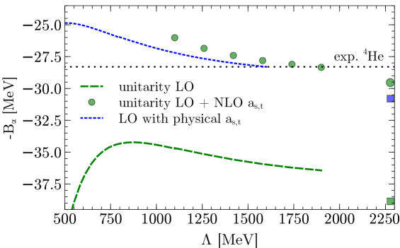
Figure 2: ${}^{4}\mathrm{He}$ binding energy as function of the Gaussian cutoff. (Blue) dotted and (green) dashed lines: standard Pionless EFT and full unitarity at LO, respectively. (Green) circles first-order corrections in $1/a_{s,t}$ added in perturbation theory. Large symbols on right edge: $\Lambda\to\infty$ extrapolation (see text).

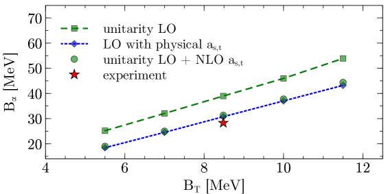
Figure 3: Tjon line: correlation between the ${}^{4}\mathrm{He}$ and ${}^{3}\mathrm{H}$ binding energies. (Blue) dotted curve: standard pionless LO result; (green) dashed upper curve: unitarity limit at LO. Additional points nearly on top of the blue curve: inverse scattering lengths added in first-order perturbation theory. Star: experimental point.

The unitarity expansion constitutes a paradigm shift in the EFT-based description of light nuclei, deemphasizing the importance of two-body details in favor of using the three-body sector as “anchor point.” As such, it is not unlike more phenomenological approaches using input from heavier nuclei in order to constrain few-nucleon forces. It is, however, much more systematic by focusing on light nuclei and strives to answer the question what really is essential to describe these systems. As discussed compellingly in Ref. [35], the idea can be boiled down to interpreting discrete scale invariance, the most striking manifestation of which is the Efimov effect, as a fundamental principle governing nuclear physics. In the bigger picture of things, the unitarity expansion furthermore stands in line with other recent results that suggest a fascinating simplification of nuclear physics. For examples, it has been observed that the isotopic chain of helium can be remarkably well described using a single-parameter model [36], and more recently a correlation analogous to the Phillips line has been observed between the $d$-$\alpha$ scattering length and the ${}^{6}\mathrm{Li}$ binding energy [37]

It is an exciting question how well the unitarity expansion works beyond what has been calculated so far. The observation that bosonic systems at unitarity exhibit saturation for large numbers of particles [38] and recent calculations of nuclear matter using interactions guided by unitarity [39] provide reasons to be optimistic. However, it remains to be seen to what extent lessons from universal bosonic systems carry over to nucleons, where beyond the four-body sector the influence of Fermi statistics is expected to become important. Concrete work looking at systems heavier than ${}^{4}\mathrm{He}$ as well as observables beyond binding energies is currently in progress.

3.0.1 Acknowledgments.

I would like to thank Harald Grießhammer, Hans-Werner Hammer, and Bira van Kolck for their collaboration as well as for many insightful discussions and comments on this manuscript. This work was supported in part by the Deutsche Forschungsgemeinschaft (DFG, German Research Foundation) – Projektnummer 279384907 – SFB 1245 and by the ERC Grant No. 307986 STRONGINT.

References

- [1] J. Schwinger, hectographed notes on nuclear physics, Harvard University (1947).
- [2] F. C. Barker and R. E. Peierls, Phys. Rev. 75 (1949) 312.
- [3] G. F. Chew and M. L. Goldberger, Phys. Rev. 75 (1949) 1637.
- [4] H. A. Bethe, Phys. Rev. 76 (1949) 38.
- [5] S. R. Beane, P. F. Bedaque, M. J. Savage and U. van Kolck, Nucl. Phys. A 700 (2002) 377.
- [6] S. R. Beane and M. J. Savage, Nucl. Phys. A 713 (2003) 148.
- [7] E. Epelbaum, U.-G. Meißner, and W. Glöckle, Nucl. Phys. A 714 (2003) 535.
- [8] S. R. Beane and M. J. Savage, Nucl. Phys. A 717 (2003) 91.
- [9] E. Braaten and H. W. Hammer, Phys. Rev. Lett. 91 (2003) 102002.
- [10] C. Chin, R. Grimm, P. Julienne, and E. Tiesinga, Rev. Mod. Phys. 82 (2010) 1225.
- [11] E. Braaten and M. Kusunoki, Phys. Rev. D 69 (2004) 074005.
- [12] V. Efimov, Phys. Lett. B 33 (1970) 563.
- [13] P. F. Bedaque, H.-W. Hammer and U. van Kolck, Phys. Rev. Lett. 82 (1999) 463.
- [14] P. F. Bedaque, H.-W. Hammer and U. van Kolck, Nucl. Phys. A 646 (1999) 444.
- [15] P. F. Bedaque, H.-W. Hammer and U. van Kolck, Nucl. Phys. A 676 (2000) 35.
- [16] W. T. H. van Oers and J. D. Seagrave, Phys. Lett. 24B (1967) 562.
- [17] B. A. Girard and M. G. Fuda, Phys. Rev. C 19 (1979) 579.
- [18] G. Rupak, A. Vaghani, R. Higa, and U. van Kolck, arXiv:1806.01999 [nucl-th].
- [19] S. K. Adhikari, A. C. Fonseca and L. Tomio, Phys. Rev. C 26 (1982) 77.
- [20] S. König, H. W. Grießhammer, H.-W. Hammer and U. van Kolck, Phys. Rev. Lett. 118 (2017) 202501.
- [21] H.-W. Hammer, S. König, and U. van Kolck, (submitted manuscript)
- [22] S. König, H. W. Grießhammer, H.-W. Hammer and U. van Kolck, J. Phys. G 43 (2016) 055106.
- [23] S. König, J. Phys. G 44 (2017) 064007.
- [24] J. Vanasse, Phys. Rev. C 88 (2013) 044001.
- [25] L. Platter, H.-W. Hammer and U.-G. Meißner, Phys. Rev. A 70 (2004) 052101.
- [26] L. Platter, H.-W. Hammer and U.-G. Meißner, Phys. Lett. B 607 (2005) 254.
- [27] L. Platter, From Cold Atoms to Light Nuclei: The Four-Body Problem in an Effective Theory with Contact Interactions, Doctoral thesis (Dissertation), University of Bonn, 2005.
- [28] L. Platter and H.-W. Hammer, Nucl. Phys. A 766 (2006) 132.
- [29] H. Kamada and W. Glöckle, Nucl. Phys. A 548 (1992) 205.
- [30] W. Glöckle, The Quantum Mechanical Few-Body Problem, Springer, Berlin (1983).
- [31] A. Stadler, W. Glockle and P. U. Sauer, Phys. Rev. C 44 (1991) 2319.
- [32] H.-W. Hammer and L. Platter, Eur. Phys. J. A 32 (2007) 113
- [33] A. Deltuva, Phys. Rev. A 82 (2010) 040701
- [34] B. Bazak, J. Kirscher, S. König, M. Pavón Valderrama, N. Barnea and U. van Kolck, arXiv:1812.00387 [cond-mat.quant-gas].
- [35] U. van Kolck, Few Body Syst. 58 (2017) 112.
- [36] K. Fossez, J. Rotureau and W. Nazarewicz, arXiv:1806.02936 [nucl-th].
- [37] J. Lei, L. Hlophe, C. Elster, A. Nogga, F. M. Nunes and D. R. Phillips, Phys. Rev. C 98 (2018) 051001.
- [38] J. Carlson, S. Gandolfi, U. van Kolck and S. A. Vitiello, Phys. Rev. Lett. 119 (2017) 223002.
- [39] A. Kievsky, M. Viviani, D. Logoteta, I. Bombaci and L. Girlanda, Phys. Rev. Lett. 121 (2018) 072701.