Electron correlation effects in enhanced-ionization of diatomic molecules in near-infrared fields

Abstract

We investigate electron correlation effects in internuclear-distance-dependent enhanced ionization of $\mathrm{H}_{2}$, $\mathrm{LiH}$, and $\mathrm{HF}$ molecules by intense near-infrared laser pulses using a 3D description of the systems with the time-dependent generalized-active-space configuration-interaction method. This method systematically incorporates electron-electron correlation of the quantum many-electron system under consideration. Our correlated description of diatomic molecules shows that enhanced ionization occurs at certain critical internuclear separations and electron correlation systematically improves the ionization probability in this process until convergence is reached. We demonstrate the failure of the single-active-electron and the configuration-interaction singles approximations to produce the correct internuclear position and probability of the strong-field enhanced-ionization process. We elucidate the role of low-lying electronic excited states in the enhanced ionization process of diatomic molecules. There is clear evidence that an accurate description of low-lying electronically excited states is important to describe the non-perturbative enhanced ionization phenomenon in the ultrashort intense near infrared laser pulses.

I Introduction

The interaction of atoms and molecules with intense laser fields gives rise to ubiquitous phenomena, such as above threshold ionization, high-harmonic generation, and enhanced ionization. With progress in experimental laser technology, it is now possible to create and observe electronic dynamics on their natural time-scale  Krausz and Ivanov (2009); Pazourek et al. (2015). Along with the experimental progress, theoreticians face the challenge to accurately describe electron-electron correlation effects in strong-field induced dynamics. Current challenges associated with the development of time-dependent methods have lead to a series of investigations for simple to complex molecular strong-field processes with both wave function Madsen et al. (2018) and density-functional theory based methods de Giovannini and Castro (2018).

In the present study, we investigate electron correlation effects in enhanced-ionization (EI) in diatomic molecules. EI describes the phenomenon that when a molecule is exposed to a strong laser field, the ionization probability increases significantly at certain critical internuclear separations. This enhancement is also known as charge-resonance enhanced ionization and has been studied extensively both experimentally  Constant et al. (1996); Pavicic et al. (2005); Ben-Itzhak et al. (2008); Bocharova et al. (2011); Wu et al. (2012); Lai and Guo (2014); Xu et al. (2015); Erattupuzha et al. (2017) and theoretically  Seideman et al. (1995); Zuo and Bandrauk (1995); Chelkowski and Bandrauk (1995); Mulyukov et al. (1996); Plummer and McCann (1996); Villeneuve et al. (1996). The quantum mechanical study of simple diatomic molecules with double-well potentials leads to many interesting features which are absent in atomic processes. It is well examined that in a double-well potential, the electron may localize in one of the potential wells with a proper choice of the laser parameters  Grossmann et al. (1991); Bavli and Metiu (1992). This mechanism may also destroy the tunneling behavior of the electron between the double wells and if the internuclear separation is increased, the localized electron may easily tunnel to the continuum from one of the potential wells as described in Ref. Seideman et al. (1995). Another mechanism explains EI as the strong coupling of charge-resonant states at certain critical internuclear separation which then leads to an enhanced molecular ionization probability  Zuo and Bandrauk (1995). Studies by numerically solving the time-dependent Schrödinger equation (TDSE) show that EI persists in two-electron homo- and heteronuclear molecules Saenz (2000, 2002); Kamta and Bandrauk (2005, 2007); Dehghanian et al. (2010, 2013). An accurate description of EI is crucial for the understanding of nuclear kinetic energy release spectra following strong-field-induced dissociative ionization (see, e.g., Ref. Jing and Madsen (2016) and references therein).

The theoretical research of time-dependent processes in many-electron systems involves solving the TDSE in the presence of strong laser fields. To tackle this problem for more than two electrons, approximations such as, e.g., the single-active-electron (SAE) Awasthi et al. (2008); Petretti et al. (2010) and the time-dependent configuration-interaction-singles (TD-CIS) approximation Rohringer et al. (2006); Greenman et al. (2010); Karamatskou et al. (2014) are needed. These approximations neglect part of the electron correlation effects in the ionization process. The present study on diatomic molecules addresses the effects of electron correlation in EI using the time-dependent generalized-active-space (TD-GASCI) method Bauch et al. (2014) in a prolate spheroidal coordinate system  Larsson et al. (2016). Over the past years, various time-dependent many-electron methods have been developed to address dynamic electron correlation in strong-field ionization of atoms and molecules. Among those, the time-dependent $R$-matrix approach  van der Hart et al. (2007); Lysaght et al. (2008, 2009); van der Hart (2014), the time-dependent Feshbach close-coupling (TDFCC) method Sanz-Vicario et al. (2006), the multiconfigurational time-dependent Hartree-Fock (MCTDHF) method  Nest et al. (2005); Caillat et al. (2005); Haxton et al. (2011, 2012); Hochstuhl et al. (2014); Greenman et al. (2017), and the time-dependent restricted-active-space self-consistent-field (TD-RAS-SCF) theory Miyagi and Madsen (2013); Sato and Ishikawa (2013); Miyagi and Madsen (2014a, b); Sato and Ishikawa (2015); Miyagi and Madsen (2017); Omiste et al. (2017); Omiste and Madsen (2018) have been used to understand dynamics. The time-dependent restricted-active-space configuration-interaction (TD-RASCI) method Hochstuhl and Bonitz (2012), and the time-dependent generalized-active-space configuration-interaction (TD-GASCI) method Bauch et al. (2014); Chattopadhyay et al. (2015); Larsson et al. (2016) take electron correlation into account through a configuration-interaction (CI) expansion by selectively choosing important Slater determinants relevant to the physical process of interest. In this method, localized Hartree-Fock and pseudo orbitals are used to represent the bound states and grid-based orbitals to obtain an accurate description of the continuum states. Depending on the construction of the generalized-active-space (GAS) one can reproduce the SAE and CIS approximations as limiting cases of the TD-GASCI method.

So far the TD-GASCI method has been used to calculate photoelectron spectra, ionization yields, structure factors for tunneling ionization, and angle-dependent ionization of one- and three-dimensional two- and four-electron atoms and molecules Bauch et al. (2014); Chattopadhyay et al. (2015); Larsson et al. (2016); Yue et al. (2017). In the present study, we employ the method to illustrate electron correlation effects in EI of diatomic molecules. First, we consider the simplest possible two-electron molecule, ${\mathrm{H}}_{2}$. This molecule has been studied extensively and we use it to check the convergence of the TD-GASCI method by comparing with exact TDSE calculations obtained from Ref. Dehghanian et al. (2010). To obtain the ionization probability we use linearly polarized laser fields with polarization parallel to the the internuclear axis within the fixed-nuclei approximation. The role of low-lying electronic excited states in EI is studied in detail. Further we consider ${\mathrm{LiH}}$ and ${\mathrm{HF}}$ molecules to highlight electron correlation effects in EI of multielectron systems. Similarly to the ${\mathrm{H}}_{2}$ case, we investigate the importance of low-lying electronic excited states in EI.

The paper is organized as follows. In Sec. II, we present the TD-GASCI method. We elaborate on the construction of the GAS partitions, define the laser pulses, discuss the calculation of the ionization probability and give some remarks on the numerical simulations, Appendix A includes more details. In Sec. III, we use the TD-GASCI method to elucidate the role of active orbitals in a given GAS partition on EI by calculating the ionization probabilities as a function of internuclear distance. We consider different GAS partitions which account for electron correlation at different levels of approximation. In Sec. IV, we summarize and conclude.

II Theory and methodology

In this section we briefly present the TD-GASCI method and its implementation in prolate spheroidal coordinates, which is discussed in details in Refs. Bauch et al. (2014); Larsson et al. (2016). Furthermore the pulses used will be given as well as the form of the complex absorbing potential.

II.1 TD-GASCI method

The TDSE for $N_{el}$ -electrons with fixed nuclei reads (we use atomic units throughout)

$$i\frac{\partial}{\partial t}|\Psi(t)\rangle=H(t)|\Psi(t)\rangle\;.$$ (1)

The time-dependent Hamiltonian consists of one- and two-body operators and is given by

$$H(t)=\sum_{i=1}^{N_{el}}{h}_{i}(t)+\sum_{i<j}^{N_{el}}w_{ij}\;,$$ (2)

with the one-body part of electron $i$ given by

$${h}_{i}(t)=-\frac{1}{2}\nabla_{i}^{2}-\frac{Z_{1}}{|\bm{r}_{i}-{\bm{R}_{1}}|}-\frac{Z_{2}}{|\bm{r}_{i}+{\bm{R}_{2}}|}+\bm{r}_{i}\cdot\bm{F}(t)\;,$$ (3)

where $\bm{F}(t)$ is the laser field and $Z_{i}(i=1,2)$ are the charges of the two nuclei. In Eq. (2), the two-body Coulomb interaction is given by

$$w_{ij}=\frac{1}{|\bm{r}_{i}-\bm{r}_{j}|}\;.$$ (4)

The many-electron wave function is expanded into a basis of time-independent Slater determinants $|\Phi_{I}\rangle$,

$$|\Psi(t)\rangle=\sum_{I\in{\cal V}_{\text{Exc}}}C_{I}(t)|\Phi_{I}\rangle\;,$$ (5)

where $C_{I}(t)$ are time-dependent expansion coefficients and $I$ is a multi-index, which specifies the configurations from the full Hilbert space ${\cal V}_{\text{Exc}}$. The Slater determinants are constructed from $N_{b}$ time-independent single-particle spatial orbitals. In terms of spin-orbitals we have 2$N_{b}$ orbitals, $\varphi_{i}(\bm{r},\sigma)$, where a given spatial orbital with different spin-quantum number has the same energy. After substituting the CI wave function from Eq. (5) into Eq. (1), the TDSE can be expressed as

$$i\frac{\partial}{\partial t}C_{I}(t)=\sum_{J\in{\cal V}_{\text{Exc}}}H_{IJ}(t)C_{J}(t)\;,$$ (6)

with the Hamiltonian matrix element, $H_{IJ}(t)=\langle\Phi_{I}|H(t)|\Phi_{J}\rangle$. These matrix elements are constructed by first evaluating the one- and two-electron integrals and then rotating the orbitals as described in Ref. Bauch et al. (2014). In the full CI (FCI) method  Szabo and Ostlund (1996); Helgaker et al. (2014) one takes into account all possible excitations ${\cal V}_{\text{Exc}}$, so that the time-dependent wave function reads

$$|\Psi_{\rm FCI}(t)\rangle = C_{0}(t)|\Phi_{0}\rangle+\sum_{ia}C_{i}^{a}(t)|\Phi_{i}^{a}\rangle$$ (7)

$$+\sum_{i<j,a<b}C_{ij}^{ab}(t)|\Phi_{ij}^{ab}\rangle+\cdots\;.$$

Here $i,j,\cdots$ refer to occupied orbitals and $a,b,\cdots$ refer to unoccupied orbitals. For example in Eq. (7), the Slater determinants in the third term, $|\Phi_{ij}^{ab}\rangle$, denote doubly excited Slater determinants where electrons from orbitals $i,j$ are excited into orbitals $a,b$. The FCI expansion is, however, numerically unfeasible even for bound state calculations for many-electron systems. In the present case we need to extract the ionization probability and it is impractical to treat all electrons with the FCI approach. This is due to the exponential scaling in the number of configurations with the number of basis functions. The GAS concept, which was introduced in quantum chemistry Olsen et al. (1988), aims to choose the most relevant configurations from the full Hilbert space for the dynamics under consideration and thus to some extend circumvents the problem of computational scaling. In the GAS method, the basis set of Slater determinants is a subset of the FCI many-particle basis set, ${\cal V}_{\text{Exc}}={\cal V}_{\text{GAS}}$ in Eq. (5). By systematically increasing the number of active orbitals, we increase the number of Slater determinants, which leads to convergence of the method towards the FCI results. This GAS approach not only reduces the computational complexity, it also allows an identification of the most important configurations for a given process and hence helps in identifying important physics.

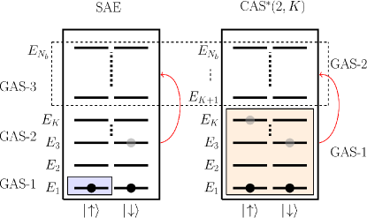
Figure 1: Schematic of GAS partitions used in this work for a two-active electron molecule. The left panel shows the SAE approximation. The right panel shows the complete-active space (CAS^∗) situation, where all single excitations out of the CAS are included. $E_{i}$ represents the orbital energy of the $i$-th orbital. The SAE approximation consists of three GAS partitions, GAS-1 defines the frozen electrons, GAS-2 defines the single-active-electron, GAS-3 defines the single excitations from GAS-2. The CAS${}^{*}(2,K)$ notation refers to two-active electrons with $K$ spatial orbitals and the asterisk denotes that all single excitations out of the active space are included. In the CAS${}^{*}(2,K)$ model we have two GAS partitions. GAS-1 contains all possible excitations within this space. GAS-2 defines single-excitation from GAS-1 to GAS-2.

In Fig. 1, we show the GAS partitions used in this work. The energies of the single-particle orbitals are denoted by $E_{i}$. The two spin configurations, $|\uparrow\rangle$ and $|\downarrow\rangle$, are degenerate in this representation. The red arrows imply that only single ionization is allowed. One can obtain the well-known SAE approximation from the GAS concept as shown in the left panel of Fig. 1. In this illustration, one of the electrons in a two-electron molecule is frozen in the GAS-1 space and the other electron is allowed to be excited within the GAS-2 space. Here we emphasize that only single excitations are allowed in the GAS-2 space, i.e., for the ionization process we allow only one-electron to be excited from GAS-2 to the GAS-3 space. The time-dependent wave function in the SAE approximation can be written as

$$|\Psi_{\rm SAE}(t)\rangle=C_{0}(t)|\Phi_{0}\rangle+\sum_{a\in vir}C_{i}^{a}(t)|\Phi_{i}^{a}\rangle\;,$$ (8)

where we note that the sum runs over all virtual orbitals. Here, $|\Phi_{0}\rangle$ is the Hartree-Fock reference determinant, and $|\Phi_{i}^{a}\rangle$ is a singly-excited determinant. Since the sum in Eq. (8) runs over all virtual orbitals, $a$, with a fixed core, $i$, it represents an effective interaction felt by the single electron, which is created by all the other electrons similar to the Hartree-Fock potential. Similarly, the explicit time-dependent wave function in the CIS approximation is described within the GAS method as

$$|\Psi_{\rm CIS}(t)\rangle=C_{0}(t)|\Phi_{0}\rangle+\sum_{i\in{\rm occ}}\sum_{a\in vir}C_{i}^{a}(t)|\Phi_{i}^{a}\rangle\;.$$ (9)

Here the sum includes all the core and virtual orbitals and all the single-excited Slater determinants are constructed with time-dependent coefficient, $C_{i}^{a}(t)$. Note that although we use the same notation for these time-dependent coefficient in Eqs. (8) and (9), they are in general different for the different approximation schemes. In the right panel of Fig. 1, we show the complete-active-space (CAS) concept Olsen et al. (1988); Bauch et al. (2014), which corresponds to a FCI description of the system with a spatial orbital index $K$. CAS${}^{*}(2,K)$ refers to two active electrons with $K(2K)$ spatial orbitals (spin orbitals) within the given CAS. In this case, all possible excitations are treated within the GAS-1 space. The asterisk denotes that all single excitations out of the CAS are included. Therefore the time-dependent wave function in the GAS method reads

$$|\Psi_{\rm CAS}(t)\rangle = C_{0}(t)|\Phi_{0}\rangle+\sum_{i\in occ}\sum_{a\in vir}C_{i}^{a}(t)|\Phi_{i}^{a}\rangle$$ (10)

$$+\sum_{i<j\in occ}\sum_{a<b\in vir}C_{ij}^{ab}(t)|\Phi_{ij}^{ab}\rangle+\cdots\;.$$

In the frozen-electron approximation, one can freeze the inner core electrons, which may have an insignificant role on the dynamics. Within the TD-GASCI method we can create such different models to describe the ionization process in a many-electron system. In this method, the restriction is created on the active space under consideration by choosing $K$ spatial orbitals and thus limiting the number of determinants within the corresponding GAS partition. We emphasize that the CAS notation throughout this work is accompanied by additional single excitations to the final GAS and indicated in our notation by CAS${}^{*}(N_{el},K)$, where $N_{el}$ denotes the active electrons and $K$ the number of spatial orbitals within the CAS under consideration.

Figure 2: Schematic of the coordinate system for diatomic molecule. The molecule with binding length $R$ has the origin in the geometric center.

II.2 Single-particle basis

The single-particle basis is constructed in the prolate spheroidal coordinate system. For a detailed description of the implementation see Refs. Larsson et al. (2016); Tao et al. (2009); Haxton et al. (2011). The coordinates are denoted by $(\xi,\eta,\phi)$, and they are related to the Cartesian coordinates by the following relations

$$\xi = \frac{r_{1}+r_{2}}{R},\quad\xi\in(1,\infty)$$

$$\eta = \frac{r_{1}-r_{2}}{R},\quad\eta\in(-1,1)$$

$$\phi = \arctan(r_{2}/r_{1}),\quad\phi\in(0,2\pi)\;.$$ (11)

Here $r_{1}$ and $r_{2}$ are the electron coordinates and $R$ is the bondlength of the diatomic molecule as shown in Fig. 2. In the prolate spheroidal coordinate system, the time-independent wave function is expressed as

$$\Psi(\xi,\eta,\phi)=\frac{1}{\sqrt{2\pi}}\sum_{m}\Psi^{m}(\xi,\eta)e^{im\phi},m=0,\pm{1},\pm{2},\cdots\;.$$ (12)

Both the $\xi$ and $\eta$-coordinates are described by a finite-element discrete-variable-representation (FE-DVR) basis Light and Carrington (2007). The total simulation box is partitioned into a central and an outer region and we use the partially rotated single-particle basis for the whole simulation box as discussed in Ref. Bauch et al. (2014); Hochstuhl et al. (2014). The $\xi$ coordinate is partitioned into two regions such that for $\xi<\xi_{s}$ the single-particle basis is constructed from localized occupied Hartree-Fock and pseudo orbitals. For $\xi>\xi_{s}$, FE-DVR functions represent the continua. The domains of these coordinates are such that ionization is mainly described by the $\xi$ coordinate, while the $\eta$ coordinate describes bound-state motion.

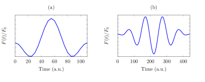
Figure 3: Normalized electric field with (a) a single cycle and (b) four-cycles.

II.3 Laser pulse parameters

To study EI, we expose diatomic molecules to 800 nm strong laser fields, which are described using the length gauge and the dipole approximation. The diatomic molecules are aligned colinearly with the polarization axis of the laser field. The vector potential has a sine-square envelope  Han and Madsen (2010),

$$A(t)=\frac{F_{0}}{\omega}\sin^{2}\Big{(}\frac{\pi t}{T}\Big{)}\sin{(\omega t)},\qquad(0\leq t\leq T)\;,$$ (13)

where $T=N\frac{2\pi}{\omega}$ is the pulse duration with $N$ the number of cycles and $\omega$ the angular frequency. The electric field is obatined as $F(t)=-\frac{\partial A(t)}{\partial t}$ and is shown in Fig. 3 for the single- ($N=1$) and four-cycle ($N=4$) pulses used in the present calculations. $F_{0}$ is the maximum amplitude of the laser pulse.The use of a vector potential to generate the electric field ensures that the time-integral over the electric field vanishes once the laser pulse is over Madsen (2002). We note that one needs a pump-probe setup to experimentally probe EI in molecules as shown in Ref. Xu et al. (2015) because the laser pulse is so short that a molecule will not have enough time to dissociate to the critical internuclear distance with EI during the duration of the pulse.

II.4 Ionization probability

To extract the total ionization probability, we add a complex absorbing potential (CAP) to the full Hamiltonian,

$$H^{\textup{CAP}}(t)=H(t)-iV_{\textup{CAP}}\;.$$ (14)

We tested various types of CAPs and found that the following CAP  Beck et al. (2000) produces a converged ionization probability for all the molecules under consideration

$$V_{\textup{CAP}}(r)=\tilde{\eta}(r-r_{\textup{CAP}})^{b}\theta(r-r_{\textup{CAP}})\;.$$ (15)

Here $\theta$ is the Heaviside step function, which ensures that the CAP is switched on once the wave packet reaches $r_{\textup{CAP}}$ and the exponent is set to $b=2$ as in Ref. Beck et al. (2000). In Eq. (15) $\tilde{\eta}$ is the CAP strength and in the present study we found converged results with $\tilde{\eta}=0.5$. Note that for the prolate-spheroidal coordinate, we apply the CAP along the $\xi$ coordinate and in all cases $\xi_{\text{CAP}}=50$. The total ionization probability Kulander (1987) reads as

$$\mathcal{P}(t_{f})=1-\mathcal{N}(t_{f})\;,$$ (16)

with $\mathcal{N}(t_{f})=\langle\Psi(t_{f})|\Psi(t_{f})\rangle$. To extract the ionization probability after the end of the pulse, we propagate the equations of motion to a final time, $t_{f}$ = 241 fs. We found that this time is sufficient to obtain converged results, also for correlated situations.

II.5 Remarks on the simulations

For the numerical simulations, first we prepare the diatomic molecule in its ground-state by imaginary-time propagation (ITP). For the ITP, we use the short-iterative Arnoldi-Lanczos algorithm Beck et al. (2000). Once the ground state is converged we apply the laser pulse and propagate in real time. We follow the adaptive time-step for the propagation of the time-dependent wave packet as discussed in Ref. Larsson et al. (2016). The EI process involves a large number of TD-GASCI simulations for different internuclear separations. Therefore, we choose a relatively large inner-region of the simulation box such that it retains the converged Hartree-Fock orbitals for the time-dependent calculations. For all the diatomic molecules that we treated, first we check the convergence of the Hartree-Fock orbitals and energies. In the time-dependent simulations we expose the diatomic molecules to 800 nm ($\omega=0.057$) laser pulses [Fig. 3]. Both the $\eta$ and $\xi$ coordinates are described by FE-DVR functions. A description of the discretization used for these variables and the computational demands is given in Appendix A.

III Results and discussion

In this section we present results on EI for H₂, LiF and HF molecules.

III.1 Two-electron $\mathrm{H}_{2}$ molecule

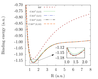
Figure 4: Ground state energy of $\mathrm{H}_{2}$ from imaginary time propagation. CAS${}^{*}(2,K)$, ($K=3,5,8,12$) represents TD-GASCI with $K$ active spatial orbitals in the CAS. In the figure, the Hartree-Fock result is denoted by HF.

In order to study correlation effects in diatomic molecules in connection with EI, the two-electron $\mathrm{H}_{2}$ molecule is a preferred choice as it is the simplest system with more than a single electron where the EI has been studied extensively by solving numerically the TDSE. First we prepare $\mathrm{H}_{2}$ in its ground state by ITP for a range of internuclear separations, $R$. In Fig. 4 we present the results with Hartree-Fock and different GAS partitions. It is seen that the CAS${}^{*}(2,3)$-calculations with three active orbitals improve the ground-state energy significantly compared to the Hartree-Fock energy. The ground-state energies from SAE and CIS approximations equal the ground-state energy of the Hartree-Fock approach due to Brillouin’s theorem  Szabo and Ostlund (1996), which states

$$\langle\Phi_{i}^{a}|H_{0}|\Phi_{0}\rangle=0\;,$$ (17)

with $H_{0}$ the time-independent field-free Hamiltonian. The CAS${}^{*}(2,5)$ scheme with five active orbitals improves the ground-state energy further. To check the convergence of the ground-state energy with the number of active orbitals, we increase the number of active orbitals in the GAS from five to eight and up to twelve for the CAS${}^{*}(2,12)$ model and one can see from the figure that the CAS${}^{*}(2,5)$ model is fully converged for the ground-state and we also obtain the correct equilibrium bond length of $R=1.4$ by the ITP method.

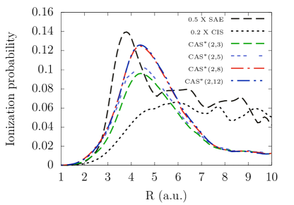
Figure 5: Ionization probability vs internuclear distance $R$ for $\mathrm{H}_{2}$ with ${F}_{0}=0.053$ and SAE, CIS and different GAS approximations. CAS${}^{*}(2,K)$, ($K=3,5,8,12$) represents $K$ active spatial orbitals in the CAS partition.

For a systematic investigation of the correlation effects in EI of $\mathrm{H}_{2}$, we use the 800 nm single-cycle laser pulse as shown in Fig. 3 (a) with a peak field strength of ${F}_{0}=0.053$ ($10^{14}$ W/cm²). For an accurate description of the correlation effects we take orbitals with higher $m$-quantum numbers as described in Eq. (12) and in the present calculations we have considered up to $m=\pm 1$ which produces a converged EI results. In Ref. Larsson et al. (2016) it was shown that $m=0,\pm 1$ is sufficient to obtain a correlated ionization spectra and further increase in $m$ does not change the ionization probability significantly. In Fig. 5, we present the ionization probability as a function of the internuclear separation. Here we scaled down the results obtained from the SAE and CIS approximations. It is evident that the SAE and CIS approximations do not produce the correct EI peak position and magnitude compared to the other correlated calculations. Also in these approximations, we observe spurious resonances as the internuclear separation is increased from $R=3.8$. In all the CAS${}^{*}(2,K)$ models in the figure, the ionization probability increases with the increase of internuclear separation and after a critical internuclear distance of $R=4.4$, it decreases and eventually at large internuclear distances equals the sum of atomic ionization probabilities. The CAS${}^{*}(2,3)$ model is the simplest model in the current description of $\mathrm{H}_{2}$ and it produces the EI-peak at the correct position, i.e, $R=4.4$. As we increase the number of active orbitals, the probability converges. Most of the correlation contributions are captured in the CAS${}^{*}(2,8)$ model. An earlier TDSE calculation produces the EI peak at a similar internuclear distance  Dehghanian et al. (2010). The same set of laser parameters produced the converged EI peak at $R=4.7$ in our previous 1D calculations  Chattopadhyay et al. (2015). A difference between the 1D and the present calculations is the way the Coulomb interaction between the electrons is treated. The regularized Coulomb potential in the 1D calculation may overestimate the correlation compared to the exact Coulomb interaction. We note that the SAE and CIS approximations are inaccurate in describing EI both in terms of magnitude and peak position. Similar conclusions were obtained from 1D calculations Chattopadhyay et al. (2015). As mentioned earlier, the TD-GASCI method systematically incorporates the electron correlation in a given GAS partition. The main difference between the SAE and CIS, and the GAS calculations is the inclusion of the doubly excited Slater determinants in the latter case. The SAE and CIS approximations are unable to describe EI because they do not include effects of double excitations in the many-electron wave function, i.e, the doubly-excited determinants ($|\Phi_{ij}^{ab}\rangle$) contribute significantly in the dynamic electron correlation which further underlines the need for correlated many-electron calculations in modeling molecular strong-field ionization processes.

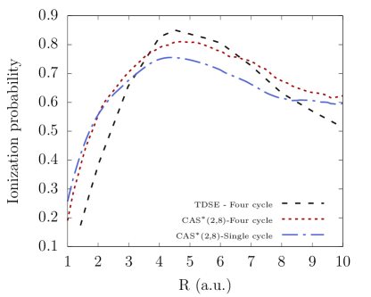
Figure 6: Comparison of the converged CAS ${}^{*}(2,8)$ TD-GASCI calculation for the ionization probabilty vs internuclear distance, $R$, for $\mathrm{H}_{2}$ with results from full 3D TDSE calculations  Dehghanian et al. (2010).

To further test the efficiency of the TD-GASCI method we consider the laser parameters from Ref. Dehghanian et al. (2010). The pulse durations are both single- and four-cycle and the peak field strength is ${F}_{0}=0.053$ ($10^{14}$ W/cm²) and $\omega=0.057$ [Fig. 3]. In Fig. 6 we compare the ionization probability of $\mathrm{H}_{2}$ as a function of the internuclear separation using the TDSE results provided in Ref. Dehghanian et al. (2010) and the converged CAS ${}^{*}(2,8)$ model of the TD-GASCI method. There is qualitative agreement between both results which further illustrates the capability of the TD-GASCI method.

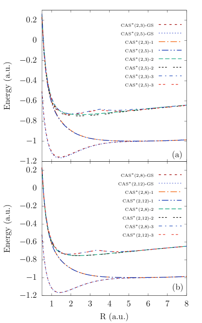
Figure 7: Field-free ground state (GS) and the three lowest-lying excited states of $\mathrm{H}_{2}$ for (a) CAS${}^{*}(2,3)$ and CAS${}^{*}(2,5)$ and (b) CAS${}^{*}(2,8)$ and CAS${}^{*}(2,12)$. The notation CAS${}^{*}(2,K)$-$i$ labels the states starting with $i=1$ for the first excited state.

The electron correlation effect in the EI of $\mathrm{H}_{2}$ is prominent from the above description. Different CAS-approximations produce the correct EI behavior but one can observe that at least eight active orbitals are required to properly describe the EI process. On the other hand one needs only five active orbitals to have a good description of the ground state. We found that the electronically excited states play an important role in the EI mechanism. This was discussed in our previous work with a 1D-$\mathrm{H}_{2}$-model molecule, and we observed a similar trend in the 3D calculations. The $K$ active orbitals in the GAS partition allow the convergence of the electronic excited states for the corresponding CAS${}^{*}(2,K)$ model and the same $K$ active orbitals are required for a converged EI calculation in the TD-GASCI method. In Fig. 7(a), we compare energies of the lowest four field-free states from CAS${}^{*}(2,3)$ and CAS${}^{*}(2,5)$ calculations. These four states are obtained by directly diagonalizing the CI-Hamiltonian in a small simulation box which also provides accurate energies. As we further increase the number of active orbitals in a GAS partition, we can see that the lowest four states converge as shown in Fig. 7(b). Thus we can see that at least eight active orbitals are required to obtain a converged result for these low-lying excited states which equals the number of states needed for the convergence of the EI process. This equality illustrates the role of electronically excited states in the EI mechanism. One can intuitively interpret that when the strong laser field is applied, the low-lying excited states can be involved in a strong coupling with the ground state at some intermediate internuclear separation and this leads to EI.

III.2 Four-electron $\mathrm{LiH}$ molecule

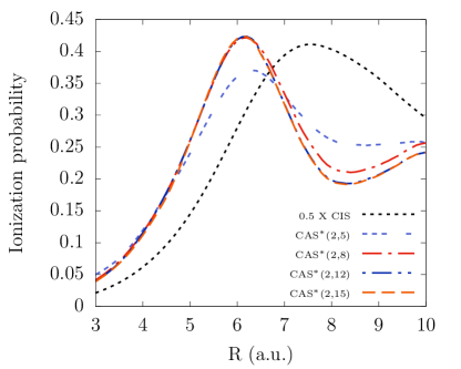
Figure 8: Ionization probability vs internuclear distance $R$ for $\mathrm{LiH}$ with ${F}_{0}=0.025$ with CIS and different GAS approximations.

In this section we present an analysis of EI in the four-electron $\mathrm{LiH}$ molecule. It is one of smallest heteronuclear systems which has been studied for electron correlation effects in both 1D and 3D calculations  Bauch et al. (2014); Chattopadhyay et al. (2015); Larsson et al. (2016). Like in the case of $\mathrm{H}_{2}$, orbitals with higher $m$-quantum numbers are needed for an accurate description of the electronic correlation and we chose up to $m=\pm 1$ for the time-dependent calculations.

We use ITP to prepare $\mathrm{LiH}$ in its ground state and then the laser pulse with a peak field strength of ${F}_{0}=0.025$ (2.18$\times 10^{13}$ W/cm²) is applied to ionize the molecule. We compare the results of EI with CIS and different GAS approximations in Fig. 8. Similar to $\mathrm{H}_{2}$, for $\mathrm{LiH}$ the CIS and all GAS approximations predict an EI peak. However, the CIS approximation predicts an incorrect EI peak position as well as magnitude compared to the other more accurate GAS approximations. This results further reflects that electron correlation effects should be taken into account to explain EI in diatomic molecules. For the CAS${}^{*}(2,5)$ scheme, the EI peak is observed at $R=5.9$. As we further increase the number of active orbitals, the peak remains at the same position but the magnitude of the ionization probability increases further until convergence is obtained with the CAS${}^{*}(2,8)$ scheme. Increasing the number of active orbitals in the GAS partitions shows the trend of convergence. Here we would also like to point out that the converged peak is shifted from $R=6.1$ in the 1D calculation Chattopadhyay et al. (2015) to $R=5.9$ in the present 3D case for the same set of laser parameters. This highlights the necessity of using the Coulomb potential instead of regularized-Coulomb potential for an accurate description of the EI process.

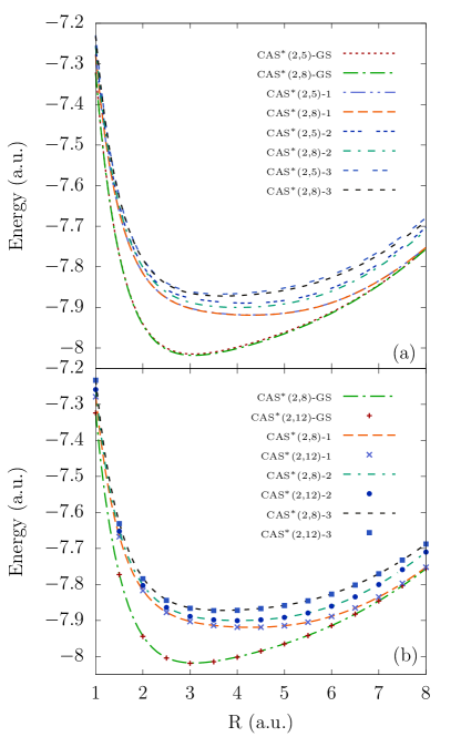
Figure 9: Field-free ground state (GS) and the three lowest-lying excited states of $\mathrm{LiH}$ for (a) CAS${}^{*}(2,5)$ and CAS${}^{*}(2,8)$ and (b) CAS${}^{*}(2,8)$ and CAS${}^{*}(2,12)$. The notation CAS${}^{*}(2,N)$-$i$ labels the states starting with $i=1$ for the first excited state.

To further study the role of electronic excited states in the EI mechanism of the $\mathrm{LiH}$ molecule we perform a diagonalization of the time-independent CI-Hamiltonian to obtain low-lying excited states. In Fig. 9(a) we show the field-free ground-state and the three lowest-lying excited states of $\mathrm{LiH}$ in CAS${}^{*}(2,5)$ and CAS${}^{*}(2,8)$ approximations. It is discernible that the CAS${}^{*}(2,5)$ model does not produce correct field-free excited states and as we increase the number of active orbitals the ground and excited states converge as shown in Fig. 9(b). Here one can see again that we need eight active orbitals in the GAS space to obtain a converged result. Note that all the energy curves are obtained with two-active electrons, i.e., with the CAS${}^{*}(2,K)$ approximations with $K$ the number of active spatial orbitals. In the ITP method, we obtain an equilibrium bond-length of $R=3.0$ for $\mathrm{LiH}$, which is very close to the value obtained by quantum chemistry calculations Helgaker et al. (2014). One can in principle use four-active electron to obtain accurate energy curves in the TD-GASCI method. However, as shown in 1D-calculations Chattopadhyay et al. (2015), the four-active electrons situation provide the EI peak at the same position as for two active electrons. Also due to higher computational cost with FE-DVR basis in both $\xi$ and $\eta$ -coordinate, we perform the imaginary and real time-propagation with two-active electrons.

III.3 Ten-electron $\mathrm{HF}$ molecule

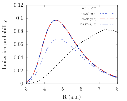
Figure 10: Ionization probability vs internuclear distance $R$ for the $\mathrm{HF}$ molecule with ${F}_{0}=0.05$ with CIS and different CAS${}^{*}(2,K)$ approximations.

One of the significant advantages of the TD-GASCI method over TDSE is the capability of a treatment of atoms and molecules with more than two electrons. To verify the universality of the EI process and electron correlation effects in strong-field ionization of multi-electron molecules, we consider the $\mathrm{HF}$ molecule.

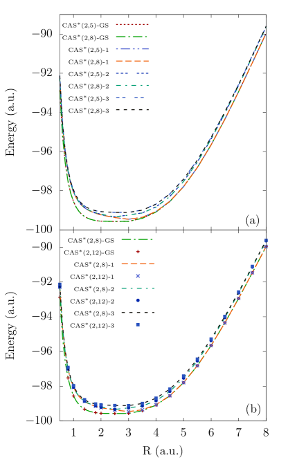
Figure 11: Field-free ground state (GS) and the three lowest-lying excited states of the $\mathrm{HF}$ molecule for (a) CAS${}^{*}(2,5)$ and CAS${}^{*}(2,8)$ and (b) CAS${}^{*}(2,8)$ and CAS${}^{*}(2,12)$. The notation CAS${}^{*}(2,N)$-$i$ labels the states starting with $i=1$ for the first excited state.

Similar to the previous cases, we prepare the $\mathrm{HF}$ molecule in its ground state with ITP method. The laser field as shown in Fig. 3 (a) is applied with a field strength of ${F}_{0}=0.05$ (8.75$\times 10^{14}$ W/cm²) to ionize the molecule. In Fig. 10, we show the ionization probability against the internuclear separation calculations for $\mathrm{HF}$. We compare the CIS approximation and different GAS methods. It is clear, like in the previous cases, that the CIS approximation fails to produce the correct EI peak position and magnitude. The present result also indicates that as the number of electrons in a system increases, the correlation effect may become more prominent. Since the CIS approximation does not take into account the doubly excited Slater determinants, it fails to incorporate a major part of the electron correlation. The present calculation further emphasizes the need of correlated time-dependent calculations for this kind of process. In the GAS schemes, we found that all the methods produce the EI peak at $R=4.6$. The lowest GAS calculation with the CAS${}^{*}(2,5)$ model predicts the correct EI peak position. As we increase the number of active orbitals, the EI peak converge with the CAS${}^{*}(2,8)$ model as in the previous cases. To check the convergence, we increase the number of active orbitals up to twelve as shown in Fig. 10 and find no significant changes in EI peak. Therefore we need eight active orbitals in this case to obtain a converged results for EI.

To study the role of electronic excited states in the EI of the $\mathrm{HF}$ molecule, we diagonalize the time-independent CI-Hamiltonian. We find the ground state and three lowest-lying excited state energies shown in Fig. 11. We note that in this case the excited states obtained from the CAS${}^{*}(2,5)$ model almost overlap with the CAS${}^{*}(2,8)$ model. We find a complete convergence of the excited states as shown in Fig. 11(b). Therefore in this case also the number of active orbitals required to produce converged excited states produce the converged EI. So we can conclude that in the near infrared region, along with the ground-state one needs an accurate representation of the low-lying excited states to obtain converged results for the EI process.

IV Summary and Conclusion

The present work highlights the role of electron correlation effects in EI of diatomic molecules. The TD-GASCI method based on the generalized-active-space concept build electron correlation in a systematic way. First we considered $\mathrm{H}_{2}$ and we found that the SAE and CIS approximations do not accurately describe EI. These two approximation even produce some spurious peaks in the EI signal. The more accurate GAS calculations produce converged ionization probabilities and we found a very good agreement with previous TDSE calculations Dehghanian et al. (2010). We demonstrated the importance of considering the double excitations in the many-electron wave function. It is remarkable that electron correlation may reduce the EI probability. We highlighted the usefulness of the TD-GASCI method which is computationally less expensive than the full TDSE treatment. The two-active electron approach was also used to treat $\mathrm{LiH}$ and $\mathrm{HF}$ molecules. We demonstrated that EI persists in these multielectron molecules and that electron correlation is necessary to obtain converged EI results. Also for these two molecules, the CIS approximation fails to predict correct EI results.

The present work is to our knowledge, the first that presents ab initio calculations on EI for system larger than $\mathrm{H}_{2}$. The results show that the EI process is universal and that correlated calculations are needed to accurately describe the process. We found that the EI results strongly depend on the convergence of the excited states. We conclude that to obtain a correct description of EI in near-infrared field, one needs an accurate representation of the ground state as well as of low-lying electronically excited states. In the future, we expect that the TD-GASCI method can be applied to study the importance of electron correlation effects in EI in mid-infrared regime.

Appendix A Numerical parameters for discretization

In this Appendix, we give details on the discretization of the prolate spheroidal coordinates and the typical CPU usages for different GAS schemes. For $\mathrm{H}_{2}$, we found that for $\xi$ two finite elements with 8 and 7 FE-DVR functions in each element with a simulation box size with $\xi_{\text{max}}=11$, 10 FE-DVR functions in $\eta$-coordinate and $m=0,\pm{1}$ is enough to obtain a converged Hartree-Fock energy and orbitals. Further increasing the number of FE-DVR functions improves the accuracy of the ground-state calculations and in this method one can reach the accuracy of different quantum chemistry calculations using a significantly higher number of FE-DVR functions within the central region. For our study of EI, we are interested in processes involving continuum dynamics and this limits the number of FE-DVR functions that can be used to construct the Hartree-Fock orbitals. For the time-dependent part we define the central region up to 11 and increase the simulation box size up to 151 in the $\xi$-coordinate. The outer region in this case consists of 28 finite elements with seven FE-DVR functions in each element. Therefore the full simulation box is of size 151 and it contains 181 basis functions in the $\xi$-coordinate. Further we use 10 FE-DVR functions in the $\eta$-coordinate and consider $m=0,\pm{1}$ for the final time-dependent simulations. So in total we have 5430 basis functions. We found that this ensures converged result for $\mathrm{H}_{2}$. We emphasize that the CAS-calculations performed in the present study are referred to as correlated CAS-calculations compared to the SAE and CIS approximations as these two approximations do not include significant contributions to the dynamic electron correlation arising from double excitations.

For all EI calculations, a single-cycle pulse has been used. Only for the comparison in Fig. 6, a four-cycle pulse was used. With the CAS${}^{*}(2,3)$ model, which is the smallest CAS calculation performed in the present work, and using the feature of the Intel MKL-library for sparse matrix-vector multiplication in a Intel Ivy-bridge processor with 20 cores at 2.8 GHz speed it takes 3 hours, 14 minutes to complete a simulation. With the CAS${}^{*}(2,12)$ model it takes 13 hours and 3 minutes to finish. For the four-electron $\mathrm{LiH}$ we found that two finite-elements with 14 and 17 FE-DVR functions with a simulation box size of 14 is sufficient to produce converged results in the central region. Similar to $\mathrm{H}_{2}$, we use 10 FE-DVR functions for the $\eta$-coordinate and we consider $m=0,\pm{1}$. For the time-dependent calculations we choose a simulation box with $\xi_{\text{max}}=150$. The total simulation box in this case has 182 FE-DVR functions for the $\xi$-coordinate and 10 FE-DVR functions for the $\eta$-coordinate and $m=0,\pm{1}$. For the full simulation box we thus have 5460 basis functions and observe converged results for all CAS-calculations. For this molecule, a time-dependent calculation with the CAS${}^{*}(2,5)$ model with the same computational configuration takes 21 hours and 7 minutes to finish. The largest CAS${}^{*}(2,15)$-scheme has taken 11 days and 1 hour and 16 minutes to obtain a converge result. In case of the $\mathrm{HF}$ molecule, we found that two finite-elements and 20 and 7 FE-DVR functions in each element for the $\xi$-coordinate and 12 FE-DVR functions in the $\eta$-coordinate and $m=0,\pm{1}$ ensure a converged Hartree-Fock energy and orbitals. For the time-dependent calculations we use a simulation box of size 101 and 133 FE-DVR functions in the $\xi$-coordinate and 12 FE-DVR functions in the $\eta$-coordinate and $m=0,\pm{1}$. The total number of basis functions in this case is 4788. A time-dependent calculation with the smallest CAS${}^{*}(2,5)$ model takes 5 days, 10 hours and 58 minutes to complete. For the largest CAS${}^{*}(2,12)$-scheme the time-dependent calculation take 21 days, 4 hours and 16 minutes to finish. The computational cost therefore restricts us to consider the four-active electron situation and in Ref. Larsson et al. (2016), it was found that for $\mathrm{LiH}$, the CAS${}^{*}(2,8)$ model produces the same ionization probability as the CAS${}^{*}(4,4)$ model. Therefore all our calculations are performed with two-active electrons.

References

- Krausz and Ivanov (2009) F. Krausz and M. Ivanov, “Attosecond physics,” Rev. Mod. Phys. 81, 163–234 (2009).
- Pazourek et al. (2015) R. Pazourek, S. Nagele, and J. Burgdörfer, “Attosecond chronoscopy of photoemission,” Rev. Mod. Phys. 87, 765–802 (2015).
- Madsen et al. (2018) L. B. Madsen, C. Lévêque, J. J. Omiste, and H. Miyagi, “Chapter 11 Time-dependent Restricted-active-space Self-consistent-field Theory for Electron Dynamics on the Attosecond Timescale,” in Attosecond Molecular Dynamics (The Royal Society of Chemistry, 2018) pp. 386–423.
- de Giovannini and Castro (2018) U. de Giovannini and A. Castro, “Chapter 12 Real-time and Real-space Time-dependent Density-functional Theory Approach to Attosecond Dynamics,” in Attosecond Molecular Dynamics (The Royal Society of Chemistry, 2018) pp. 424–461.
- Constant et al. (1996) E. Constant, H. Stapelfeldt, and P. B. Corkum, “Observation of enhanced ionization of molecular ions in intense laser fields,” Phys. Rev. Lett. 76, 4140–4143 (1996).
- Pavicic et al. (2005) D. Pavicic, A. Kiess, T. W. Hänsch, and H. Figger, “Intense-laser-field ionization of the hydrogen molecular ions and at critical internuclear distances,” Phys. Rev. Lett. 94, 163002 (2005).
- Ben-Itzhak et al. (2008) I. Ben-Itzhak, P. Q. Wang, A. M. Sayler, K. D. Carnes, M. Leonard, B. D. Esry, A. S. Alnaser, B. Ulrich, X. M. Tong, I. V. Litvinyuk, C. M. Maharjan, P. Ranitovic, T. Osipov, S. Ghimire, Z. Chang, and C. L. Cocke, “Elusive enhanced ionization structure for in intense ultrashort laser pulses,” Phys. Rev. A 78, 063419 (2008).
- Bocharova et al. (2011) I. Bocharova, R. Karimi, E. F. Penka, J. Brichta, P. Lassonde, X. Fu, J. Kieffer, A. D. Bandrauk, I. Litvinyuk, J. Sanderson, and F. Légaré, “Charge resonance enhanced ionization of probed by laser coulomb explosion imaging,” Phys. Rev. Lett. 107, 063201 (2011).
- Wu et al. (2012) J. Wu, M. Meckel, L.Ph.H. Schmidt, M. Kunitski, S. Voss, H. Sann, H. Kim, T. Jahnke, A. Czasch, and R. Dörner, “Probing the tunnelling site of electrons in strong field enhanced ionization of molecules,” Nat. Commun. 3, 1113 (2012).
- Lai and Guo (2014) W. Lai and C. Guo, “Direct detection of enhanced ionization in and in strong fields,” Phys. Rev. A 90, 031401(R) (2014).
- Xu et al. (2015) H. Xu, F. He, D. Kielpinski, R. T. Sang, and I. V. Litvinyuk, “Experimental observation of the elusive double-peak structure in R-dependent strong-field ionization rate of ,” Scientific Reports 5, 13527 (2015).
- Erattupuzha et al. (2017) S. Erattupuzha, C. L. Covington, A. Russakoff, E. Lötstedt, S. Larimian, V. Hanus, S. Bubin, M. Koch, S. Gräfe, A. Baltuška, X. Xie, K. Yamanouchi, K. Varga, and M. Kitzler, “Enhanced ionisation of polyatomic molecules in intense laser pulses is due to energy upshift and field coupling of multiple orbitals,” Journal of Physics B: Atomic, Molecular and Optical Physics 50, 125601 (2017).
- Seideman et al. (1995) T. Seideman, M. Yu. Ivanov, and P. B. Corkum, “Role of electron localization in intense-field molecular ionization,” Phys. Rev. Lett. 75, 2819–2822 (1995).
- Zuo and Bandrauk (1995) T. Zuo and A. D. Bandrauk, “Charge-resonance-enhanced ionization of diatomic molecular ions by intense lasers,” Phys. Rev. A 52, R2511–R2514 (1995).
- Chelkowski and Bandrauk (1995) S. Chelkowski and A. D. Bandrauk, “Two-step coulomb explosions of diatoms in intense laser fields,” Journal of Physics B: Atomic, Molecular and Optical Physics 28, L723 (1995).
- Mulyukov et al. (1996) Z. Mulyukov, M. Pont, and R. Shakeshaft, “Ionization, dissociation, and level shifts of in a strong dc or low-frequency ac field,” Phys. Rev. A 54, 4299–4308 (1996).
- Plummer and McCann (1996) M. Plummer and J. F. McCann, “Field-ionization rates of the hydrogen molecular ion,” Journal of Physics B: Atomic, Molecular and Optical Physics 29, 4625 (1996).
- Villeneuve et al. (1996) D. M. Villeneuve, M. Yu. Ivanov, and P. B. Corkum, “Enhanced ionization of diatomic molecules in strong laser fields: A classical model,” Phys. Rev. A 54, 736–741 (1996).
- Grossmann et al. (1991) F. Grossmann, T. Dittrich, P. Jung, and P. Hänggi, “Coherent destruction of tunneling,” Phys. Rev. Lett. 67, 516–519 (1991).
- Bavli and Metiu (1992) R. Bavli and H. Metiu, “Laser-induced localization of an electron in a double-well quantum structure,” Phys. Rev. Lett. 69, 1986–1988 (1992).
- Saenz (2000) A. Saenz, “Enhanced ionization of molecular hydrogen in very strong fields,” Phys. Rev. A 61, 051402(R) (2000).
- Saenz (2002) A. Saenz, “Behavior of molecular hydrogen exposed to strong dc, ac, or low-frequency laser fields. i. bond softening and enhanced ionization,” Phys. Rev. A 66, 063407 (2002).
- Kamta and Bandrauk (2005) G. L. Kamta and A. D. Bandrauk, “Phase dependence of enhanced ionization in asymmetric molecules,” Phys. Rev. Lett. 94, 203003 (2005).
- Kamta and Bandrauk (2007) G. L. Kamta and A. D. Bandrauk, “Nonsymmetric molecules driven by intense few-cycle laser pulses: Phase and orientation dependence of enhanced ionization,” Phys. Rev. A 76, 053409 (2007).
- Dehghanian et al. (2010) E. Dehghanian, A. D. Bandrauk, and G. L. Kamta, “Enhanced ionization of the molecule driven by intense ultrashort laser pulses,” Phys. Rev. A 81, 061403(R) (2010).
- Dehghanian et al. (2013) E. Dehghanian, A. D. Bandrauk, and G. L. Kamta, “Enhanced ionization of the non-symmetric heh+ molecule driven by intense ultrashort laser pulses,” The Journal of Chemical Physics 139, 084315 (2013).
- Jing and Madsen (2016) Q. Jing and L. B. Madsen, “Laser-induced dissociative ionization of from the near-infrared to the mid-infrared regime,” Phys. Rev. A 94, 063402 (2016).
- Awasthi et al. (2008) M. Awasthi, Y. V. Vanne, A. Saenz, A. Castro, and P. Decleva, “Single-active-electron approximation for describing molecules in ultrashort laser pulses and its application to molecular hydrogen,” Phys. Rev. A 77, 063403 (2008).
- Petretti et al. (2010) S. Petretti, Y. V. Vanne, A. Saenz, A. Castro, and P. Decleva, “Alignment-dependent ionization of , , and in intense laser fields,” Phys. Rev. Lett. 104, 223001 (2010).
- Rohringer et al. (2006) N. Rohringer, A. Gordon, and R. Santra, “Configuration-interaction-based time-dependent orbital approach for ab initio treatment of electronic dynamics in a strong optical laser field,” Phys. Rev. A 74, 043420 (2006).
- Greenman et al. (2010) L. Greenman, Phay J. Ho, S. Pabst, E. Kamarchik, D. A. Mazziotti, and R. Santra, “Implementation of the time-dependent configuration-interaction singles method for atomic strong-field processes,” Phys. Rev. A 82, 023406 (2010).
- Karamatskou et al. (2014) A. Karamatskou, S. Pabst, Y. J. Chen, and R. Santra, “Calculation of photoelectron spectra within the time-dependent configuration-interaction singles scheme,” Phys. Rev. A 89, 033415 (2014).
- Bauch et al. (2014) S. Bauch, L. K. Sørensen, and L. B. Madsen, “Time-dependent generalized-active-space configuration-interaction approach to photoionization dynamics of atoms and molecules,” Phys. Rev. A 90, 062508 (2014).
- Larsson et al. (2016) H. R. Larsson, S. Bauch, L. K. Sørensen, and M. Bonitz, “Correlation effects in strong-field ionization of heteronuclear diatomic molecules,” Phys. Rev. A 93, 013426 (2016).
- van der Hart et al. (2007) H. W. van der Hart, M. A. Lysaght, and P. G. Burke, “Time-dependent multielectron dynamics of ar in intense short laser pulses,” Phys. Rev. A 76, 043405 (2007).
- Lysaght et al. (2008) M. A. Lysaght, P. G. Burke, and H. W. van der Hart, “Ultrafast laser-driven excitation dynamics in Ne: An ab initio time-dependent R-matrix approach,” Phys. Rev. Lett. 101, 253001 (2008).
- Lysaght et al. (2009) M. A. Lysaght, H. W. van der Hart, and P. G. Burke, “Time-dependent R-matrix theory for ultrafast atomic processes,” Phys. Rev. A 79, 053411 (2009).
- van der Hart (2014) H. W. van der Hart, “Time-dependent R-matrix theory applied to two-photon double ionization of He,” Phys. Rev. A 89, 053407 (2014).
- Sanz-Vicario et al. (2006) J. L. Sanz-Vicario, H. Bachau, and F. Martín, “Time-dependent theoretical description of molecular autoionization produced by femtosecond xuv laser pulses,” Phys. Rev. A 73, 033410 (2006).
- Nest et al. (2005) M. Nest, T. Klamroth, and P. Saalfrank, “The multiconfiguration time-dependent Hartree-Fock method for quantum chemical calculations,” J. Chem. Phys. 122, 124102 (2005).
- Caillat et al. (2005) J. Caillat, J. Zanghellini, M. Kitzler, O. Koch, W. Kreuzer, and A. Scrinzi, “Correlated multielectron systems in strong laser fields: A multiconfiguration time-dependent hartree-fock approach,” Phys. Rev. A 71, 012712 (2005).
- Haxton et al. (2011) D. J. Haxton, K. V. Lawler, and C. W. McCurdy, “Multiconfiguration time-dependent hartree-fock treatment of electronic and nuclear dynamics in diatomic molecules,” Phys. Rev. A 83, 063416 (2011).
- Haxton et al. (2012) D. J. Haxton, K. V. Lawler, and C. W. McCurdy, “Single photoionization of be and hf using the multiconfiguration time-dependent hartree-fock method,” Phys. Rev. A 86, 013406 (2012).
- Hochstuhl et al. (2014) D. Hochstuhl, C.M. Hinz, and M. Bonitz, “Time-dependent multiconfiguration methods for the numerical simulation of photoionization processes of many-electron atoms,” The European Physical Journal Special Topics 223, 177–336 (2014).
- Greenman et al. (2017) L. Greenman, K. B. Whaley, D. J. Haxton, and C. W. McCurdy, “Optimized pulses for raman excitation through the continuum: Verification using the multiconfigurational time-dependent hartree-fock method,” Phys. Rev. A 96, 013411 (2017).
- Miyagi and Madsen (2013) H. Miyagi and L. B. Madsen, “Time-dependent restricted-active-space self-consistent-field theory for laser-driven many-electron dynamics,” Phys. Rev. A 87, 062511 (2013).
- Sato and Ishikawa (2013) T. Sato and K. L. Ishikawa, “Time-dependent complete-active-space self-consistent-field method for multielectron dynamics in intense laser fields,” Phys. Rev. A 88, 023402 (2013).
- Miyagi and Madsen (2014a) H. Miyagi and L. B. Madsen, “Time-dependent restricted-active-space self-consistent-field singles method for many-electron dynamics,” J. Chem. Phys. 140, 164309 (2014a).
- Miyagi and Madsen (2014b) H. Miyagi and L. B. Madsen, “Time-dependent restricted-active-space self-consistent-field theory for laser-driven many-electron dynamics. ii. extended formulation and numerical analysis,” Phys. Rev. A 89, 063416 (2014b).
- Sato and Ishikawa (2015) T. Sato and K. L. Ishikawa, “Time-dependent multiconfiguration self-consistent-field method based on the occupation-restricted multiple-active-space model for multielectron dynamics in intense laser fields,” Phys. Rev. A 91, 023417 (2015).
- Miyagi and Madsen (2017) H. Miyagi and L. B. Madsen, “Time-dependent restricted-active-space self-consistent-field theory with space partition,” Phys. Rev. A 95, 023415 (2017).
- Omiste et al. (2017) J. J. Omiste, W. Li, and L. B. Madsen, “Electron correlation in beryllium: Effects in the ground state, short-pulse photoionization, and time-delay studies,” Phys. Rev. A 95, 053422 (2017).
- Omiste and Madsen (2018) J. J. Omiste and L. B. Madsen, “Attosecond photoionization dynamics in neon,” Phys. Rev. A 97, 013422 (2018).
- Hochstuhl and Bonitz (2012) D. Hochstuhl and M. Bonitz, “Time-dependent restricted-active-space configuration-interaction method for the photoionization of many-electron atoms,” Phys. Rev. A 86, 053424 (2012).
- Chattopadhyay et al. (2015) S. Chattopadhyay, S. Bauch, and L. B. Madsen, “Electron-correlation effects in enhanced ionization of molecules: A time-dependent generalized-active-space configuration-interaction study,” Phys. Rev. A 92, 063423 (2015).
- Yue et al. (2017) L. Yue, S. Bauch, and L. B. Madsen, “Electron correlation in tunneling ionization of diatomic molecules: An application of the many-electron weak-field asymptotic theory with a generalized-active-space partition scheme,” Phys. Rev. A 96, 043408 (2017).
- Szabo and Ostlund (1996) A. Szabo and N. S. Ostlund, Modern Quantum Chemistry: Introduction to Advanced Electronic Structure Theory (Dover Publications, 1996).
- Helgaker et al. (2014) T. Helgaker, P. Jørgensen, and J. Olsen, Molecular Electronic-Structure Theory (Wiley, 2014).
- Olsen et al. (1988) J. Olsen, B. O. Roos, P. Jørgensen, and H. J. Aa. Jensen, “Determinant based configuration interaction algorithms for complete and restricted configuration interaction spaces,” J. Chem. Phys. 89, 2185–2192 (1988).
- Tao et al. (2009) L. Tao, C. W. McCurdy, and T. N. Rescigno, “Grid-based methods for diatomic quantum scattering problems: A finite-element discrete-variable representation in prolate spheroidal coordinates,” Phys. Rev. A 79, 012719 (2009).
- Light and Carrington (2007) J. C. Light and T. Carrington, “Discrete-variable representations and their utilization,” in Advances in Chemical Physics (John Wiley & Sons, Ltd, 2007) pp. 263–310.
- Han and Madsen (2010) Y-C. Han and L. B. Madsen, “Comparison between length and velocity gauges in quantum simulations of high-order harmonic generation,” Phys. Rev. A 81, 063430 (2010).
- Madsen (2002) L. B. Madsen, “Gauge invariance in the interaction between atoms and few-cycle laser pulses,” Phys. Rev. A 65, 053417 (2002).
- Beck et al. (2000) M. H. Beck, A. Jäckle, G. A. Worth, and H.-D. Meyer, “The multiconfiguration time-dependent hartree (MCTDH) method: a highly efficient algorithm for propagating wavepackets,” Phys. Rep. 324, 1 – 105 (2000).
- Kulander (1987) K. C. Kulander, “Multiphoton ionization of hydrogen: A time-dependent theory,” Phys. Rev. A 35, 445–447 (1987).