Measurement of Tidal Deformability in the Gravitational Wave Parameter Estimation for Nonspinning Binary Neutron Star Mergers

Abstract

One of the main targets for ground-based gravitational wave (GW) detectors such as Advanced LIGO (Laser Interferometer Gravitational wave Observatory) and Virgo is coalescences of neutron star (NS) binaries. Even though a NS’s macroscopic properties such as mass and radius have been obtained from electro-magnetic wave observations, its internal structure has been studied mainly by using theoretical approaches. However, with the advent of Advanced LIGO and Virgo, the tidal deformability of a NS, which depends on the internal structure of the NS, has been recently obtained from GW observations. Therefore, reducing the measurement error of tidal deformability as small as possible in the GW parameter estimation is important. In this study, we introduce a post-Newtonian (PN) gravitational waveform model in which the tidal deformability contribution appears from 5 PN order, and we use the Fisher matrix (FM) method to calculate parameter measurement errors. Because the FM is computed semi-analytically using the wave function, the measurement errors can be obtained much faster than those of practical parameter estimations based on Markov Chain Monte Carlo method. We investigate the measurement errors for mass and tidal deformability by applying the FM to the nonspinning TaylorF2 waveform model. We show that if the tidal deformability corrections are considered up to the 6 PN order, the measurement error for the dimensionless tidal deformability can be reduced to about $75\%$ compared to that obtained by considering only the 5 PN order correction.

I INTRODUCTION

The presence of gravitational waves (GWs) was predicted by Einstein in 1916 Einstein1916 and 1918 Einstein1918 . The strain of GWs, however, is extremely small; hence, numerous efforts over the past decades to detect real GWs have failed. Finally, the first GW signal, named as GW150914, was captured by the two Advanced LIGO (Laser Interferometer Gravitational wave Observatory) detectors in September 2015. During the first and the second observing runs of the network of Advanced LIGO and Virgo, a total of 10 GW signals from binary black hole mergers were detected Abbott16 ; Abbott16_2 ; Abbott17 ; Abbott17_2 ; Abbott17_3 ; GWCatalog_1 ; GWCatalog_2 . Eventually, a multi-messenger astronomy era began with the observation of a GW signal from a binary neutron star (NS) merger in 2017 Abbott17_4 ; Abbott17_5 . Because KAGRA is planning to join the third observing run Somiya12 ; Akutsu17 , the expected detection rate of binary NS mergers is 3.2 $\sim$ 9.2 times per year with the four-detector network Dominik15 .

One of the main targets of Advanced LIGO and Virgo is compact binary coalescences (CBCs) in which a compact binary means a black hole-black hole, black hole-NS, or NS-NS binary. In data analysis for GWs from CBCs, a signal can be distinguished from noise by matching the detector data with theoretical waveforms. Once a GW signal is identified in the detection pipeline, a more detailed analysis can be carried out in the parameter estimation pipeline based on the Markov Chain Monte Carlo method. While the main purpose of the GW detection pipeline is to decide whether the GW signal enters the data stream or not, the parameter estimation pipeline seeks source properties such as the mass and the spin of the system. The result of the parameter estimation analysis is given by probability density functions for the parameters considered, and this process typically requires a very long time and a large amount of computing resources. On the other hand, if the incident GW signal is strong enough and buried in Gaussian noise, the measurement errors can be easily calculated by using the Fisher matrix (FM) method, which is a semi-analytic approach used to approximate the accuracy of the parameter estimation.

Recently, the tidal deformability of a NS was measured from the GWs generated by the merger of a neutron star binary Abbott17_4 ; GW170817EOS . This parameter describes the response of a NS to the external tidal field generated by its companion star. In the current GW parameter estimations, the observational constraints on the NS radii are well estimated; however, the measurement errors for tidal deformability are not small enough to precisely distinguish various equations of state (EOSs) Abbott17_4 ; GW170817EOS .

In this work, we introduce a post-Newtonian (PN) waveform model, which is expressed in the frequency domain and is valid for the inspiral waveforms emitted from CBCs. This model incorporates 3.5 PN order point-particle contributions and 5 PN and 6 PN tidal corrections. We use the FM method and calculate the measurement errors of the mass and the tidal parameters for a nonspinning, equal-mass binary NS assuming the Advanced LIGO detector sensitivity. We investigate how much the 6 PN tidal correction can improve the accuracy in measuring the tidal deformability.

II Post-newtonian Gravitational waveforms

The physical parameters used to define waveforms from CBC systems are divided into two groups. One group includes intrinsic parameters such as mass and spin, which are directly related to the dynamics of a binary and the shape of the waveform. The other includes extrinsic parameters such as luminosity distance, sky position, and inclination of the orbital axis. Unlike the intrinsic parameters, the extrinsic parameters only affect the wave amplitude; hence, they do not need to be considered in our analysis. Generally, the correlation values between intrinsic and extrinsic parameters are much less than those between the intrinsic parameters Raymond12 .

The dynamics of CBCs in the relativistic region can be calculated using numerical simulations, which typically require a large amount of computing resources. However, in the region of slow orbital velocity ($v_{0}/c\ll 1$) and weak gravitational field ($GM/(rc^{2})\ll 1$), the post-Newtonian (PN) approximation is good enough to describe the CBC dynamics and model the gravitational waveforms from the CBC inspirals; hence, much fewer computing resources are required.

The frequency-domain PN waveform model obtained by using the stationary-phase approximation is called TaylorF2. The TaylorF2 waveform can be written as

$$\tilde{h}(f)=Af^{-7/6}e^{i\psi(f)},$$ (1)

where $A$ is the wave amplitude consisting of the chirp mass ($M_{c}\equiv(m_{1}m_{2})^{3/5}/M^{1/5}$, where $M$ is the total mass) and the extrinsic parameters. The phase $\psi(f)$ is expressed as the PN expansion

$$\psi(f)=2\pi ft_{c}-\phi_{c}-\frac{\pi}{4}+\frac{3}{128\eta v^{5}}\bigg{(}\Psi_{\rm 3.5PN}^{\rm PP}+\Psi^{\rm Tidal}\bigg{)},$$ (2)

where $t_{c}$ and $\phi_{c}$ are the coalescence time and the coalescence phase, respectively, which can be chosen arbitrarily, $\eta\equiv m_{1}m_{2}/M^{2}$ is the symmetric mass ratio, and $v\equiv(\pi GMf)^{1/3}/c$ is the characteristic velocity. In the bracket, $\Psi_{\rm 3.5PN}^{\rm PP}$ is the point-particle contribution incorporated up to 3.5 PN order Buonanno09 , and $\Psi^{\rm Tidal}$ is the contribution by the quadrupolar tidal interaction, which is discussed in the next section.

III Tidal deformability

In a merging binary NS system, one NS can be deformed by the tidal field generated by the companion NS. To linear order, the quadrupole moment $Q_{ij}$ induced by the external quadrupolar tidal field $\mathcal{E}_{ij}$ is given by Flanagan08 ; Lackey12

$$Q_{ij}=-\lambda\mathcal{E}_{ij},$$ (3)

which can be decomposed with the symmetric traceless tensor $\mathcal{Y}^{lm}_{ij}$ defined by spherical harmonics $Y_{lm}(\theta,\phi)$ Hinderer09 . Only the leading contribution $l=2$ is included in our consideration; thus, the constant $\lambda$ is the $l=2$ tidal deformability. The quadrupole moment is related to density perturbation $\delta\rho$ as

$$Q_{ij}=\int d^{3}x~{}\delta\rho(x)~{}(x_{i}x_{j}-\delta_{ij}r^{2}/3),$$ (4)

and $\mathcal{E}_{ij}$ can be expressed in terms of the external gravitational potential $\Phi_{\rm ext}$ as

$$\mathcal{E}_{ij}=\frac{\partial^{2}\Phi_{\rm ext}}{\partial x^{i}\partial x^{j}}.$$ (5)

The tidal deformability is defined by Hinderer09 ; Flanagan08

$$\lambda=\frac{2}{3G}k_{2}R^{5},$$ (6)

where $k_{2}$ is the Love number and $R$ is a radius of the NS. For a given NS mass, the tidal deformability can vary according to the EOSs Hinderer10 .

In a binary NS system, the tidal deformability contribution is given up to 6 PN order as Lackey15

$$\Psi^{\rm Tidal}(f)=-\bigg{[}\frac{39\tilde{\Lambda}}{2}v^{10}+\bigg{(}\frac{3115\tilde{\Lambda}}{64}-\frac{6595\sqrt{1-4\eta}~{}\delta\tilde{\Lambda}}{364}\bigg{)}v^{12}\bigg{]},$$ (7)

where the reduced tidal deformability $\tilde{\Lambda}$ and the asymmetric tidal correction $\delta\tilde{\Lambda}$ are defined as Lackey15

$$\tilde{\Lambda} = 32\frac{c^{10}\tilde{\lambda}}{G^{4}M^{5}}$$ (8)

$$= \frac{16c^{10}}{13G^{4}}\bigg{(}\frac{m_{1}+12m_{2}}{m_{1}}\lambda_{1}+\frac{m_{2}+12m_{1}}{m_{2}}\lambda_{2}\bigg{)}$$

$$= \frac{8}{13}[(1+7\eta-31\eta^{2})(\Lambda_{1}+\Lambda_{2})$$

$$+ \sqrt{1-4\eta}(1+9\eta-11\eta^{2})(\Lambda_{1}-\Lambda_{2})],$$

$$\delta\tilde{\Lambda} = \frac{1}{2}\bigg{[}\sqrt{1-4\eta}\bigg{(}1-\frac{13272\eta}{1319}+\frac{8944\eta^{2}}{1319}\bigg{)}(\Lambda_{1}+\Lambda_{2})$$

$$+ \bigg{(}1-\frac{15910\eta}{1319}+\frac{32850\eta^{2}}{1319}+\frac{3380\eta^{3}}{1319}\bigg{)}(\Lambda_{1}-\Lambda_{2})\bigg{]},$$

where $m_{1}\geq m_{2}$, and $\Lambda_{i}=c^{10}\lambda_{i}/(G^{4}{m_{i}}^{5})$ is the dimensionless tidal deformability of a single star. The subscripts 1 and 2 indicate the individual NSs. Because $\Lambda_{1}$ and $\Lambda_{2}$ are strongly correlated, $\tilde{\Lambda}$ and $\delta\tilde{\Lambda}$ are much more efficient in most analyses. Typically, $\delta\tilde{\Lambda}/\tilde{\Lambda}$ is about 0.01; hence, the contribution of $\delta\tilde{\Lambda}$ is negligible Favata14 . In this work, we assume $m_{1}=m_{2}$ and $\Lambda_{1}=\Lambda_{2}$; then, $\tilde{\Lambda}=\Lambda_{1}=\Lambda_{2}$ and the $\delta\tilde{\Lambda}$ term vanishes in Eq. (7).

IV measurement error

Once a detection is made in the detection pipeline, the parameter estimation pipeline seeks the source parameters based on Markov Chain Monte Carlo method. Although it is guaranteed to converge, this method typically requires a long computational time. On the other hand, the FM method has generally been used to predict accuracy of the parameter estimation approximately for high signal-to-noise ratio (SNR) signals Cho14 ; Cho15-1 (for a general overview of the FM, refer to Vallisneri08 ). The FM can be calculated semi-analytically by using the post-Newtonian waveform; therefore, the measurement errors can be obtained much faster than those of practical parameter estimation.

For a given theoretical waveform $h(t)$ and detector data stream $x(t)$ that can contain a real GW strain, the likelihood is determined by Cutler94 ; Finn92

$$L(x|\theta)=\exp[-\langle x-h(\theta)|x-h(\theta)\rangle/2],$$ (10)

where $\theta$ is a physical parameter set including a chirp mass and a symmetric mass ratio, etc. In the above, $\langle x|h\rangle$ means the noise-weighted inner product given by

$$\langle x|h\rangle=2\int_{f_{\rm min}}^{f_{\rm max}}\frac{\tilde{x}^{*}(f)\tilde{h}(f)+\tilde{x}(f)\tilde{h}^{*}(f)}{S_{n}(f)}df,$$ (11)

where $f_{\rm min}$ and $f_{\rm max}$ are the minimum and the maximum cutoff frequencies, respectively, and $S_{n}(f)$ is the noise power spectral density of the detector.

In the high SNR limit, the likelihood can be expressed as Cutler94 ; Cho13

$$L(\theta) \propto \exp[-\rho^{2}\{1-\langle\hat{h}_{0}|\hat{h}(\theta)\rangle\}]$$ (12)

$$= {\exp}[-\Gamma_{ij}\Delta\theta_{i}\Delta\theta_{j}/2],$$

where $\hat{h}$ denotes the normalized waveform, $\hat{h}\equiv h/\sqrt{\langle h|h\rangle}$, $\rho$ is the SNR, $\rho\equiv\sqrt{\langle h_{0}|h_{0}\rangle}$, $h_{0}$ is the GW signal, and $\Gamma_{ij}$ is the FM defined by

$$\Gamma_{ij}=\bigg{\langle}\frac{\partial h}{\partial\theta_{i}}\bigg{|}\frac{\partial h}{\partial\theta_{j}}\bigg{\rangle}\bigg{|}_{\theta_{i}=\theta_{\rm true}}.$$ (13)

The inverse of the FM corresponds to the covariance matrix of parameter errors. Thus, the measurement error $\sigma_{i}$ and the correlation coefficient $c_{ij}$ can be determined by using

$$\sigma_{i}=\sqrt{(\Gamma^{-1})_{ii}},\\ {c}_{ij}=\frac{(\Gamma^{-1})_{ij}}{\sqrt{(\Gamma^{-1})_{ii}(\Gamma^{-1})_{jj}}}.$$ (14)

V Result

We adopt a nonspinning equal-mass binary NS with $m_{1}=m_{2}=1.4M_{\odot}$ and choose $\Lambda_{1}=\Lambda_{2}=300$ following the result in GW170817EOS . We consider the Advanced LIGO noise curve given in Ajith09 and assume $f_{\rm min}$ = 10 Hz. By using the TaylorF2 waveform, we calculate the 5$\times$5 FM whose components are $\theta_{i}$={${M_{c}},\eta,\tilde{\Lambda},{t_{c}},{\phi_{c}}\}$ and present the measurement errors $\sigma_{M_{c}},\sigma_{\eta}$, and $\sigma_{\tilde{\Lambda}}$.

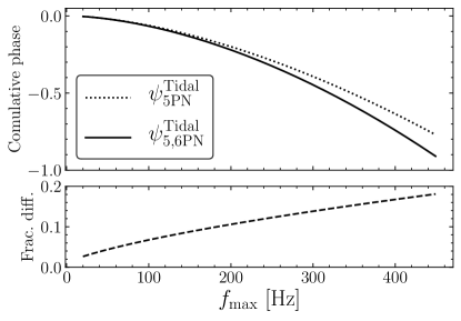
Figure 1: The cumulative phase due to the tidal terms $\psi^{\rm Tidal}_{\rm 5PN}$ and $\psi^{\rm Tidal}_{\rm 5,6PN}$ (upper panel) and their fractional difference $(\psi^{\rm Tidal}_{\rm 5,6PN}-\psi^{\rm Tidal}_{\rm 5PN})/\psi^{\rm Tidal}_{\rm 5PN}$ (lower panel). We assume $f_{\rm min}=10$.

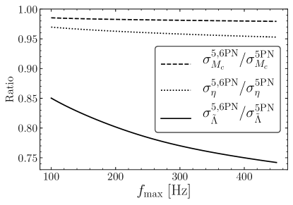
Figure 2: Ratio of the measurement errors between the $\psi^{\rm Tidal}_{\rm 5PN}$ and the $\psi^{\rm Tidal}_{\rm 5,6PN}$ waveform cases (see text). We adopt a nonspinning equal-mass binary NS with $m_{1}=m_{2}=1.4M_{\odot}$ and $\Lambda_{1}=\Lambda_{2}=300$. We consider the Advanced LIGO noise curve and assume $f_{\rm min}$ = 10 Hz. Note that the measurement error of $\tilde{\Lambda}$ can be reduced to about $75\%$ at $450$ Hz by taking into account the tidal correction up to 6 PN compared to the case in which only the 5 PN tidal correction is considered.

Figure 1 shows the cumulative phases from $10$ Hz to $f_{\rm max}$ due to the 5 PN tidal term ($\psi^{\rm Tidal}_{\rm 5PN}$) and the sum of the 5 PN and the 6 PN tidal terms ($\psi^{\rm Tidal}_{\rm 5,6PN}$), respectively. The fractional difference ($(\psi^{\rm Tidal}_{\rm 5,6PN}-\psi^{\rm Tidal}_{\rm 5PN})/\psi^{\rm Tidal}_{\rm 5PN}$) is also given in Figure 1. We show the result only up to 450 Hz because our TaylorF2 model is fairly valid to 450 Hz Hinderer10 . Note that the fractional difference is about $20\%$ at $450$ Hz.

Next, we investigate how the 6 PN tidal term contributes to improving the accuracy in measuring the tidal parameter $\tilde{\Lambda}$. We take into account $\psi^{\rm Tidal}_{\rm 5PN}$ and $\psi^{\rm Tidal}_{\rm 5,6PN}$ in Eq. (2) and calculate the measurement errors for both cases. Figure 2 shows the ratio of the measurement errors between the $\psi^{\rm Tidal}_{\rm 5PN}$ and the $\psi^{\rm Tidal}_{\rm 5,6PN}$ waveform cases. One can see that the measurement accuracy of the tidal deformability is significantly improved by including the 6 PN tidal correction. In this case, the measurement error of $\tilde{\Lambda}$ can be reduced to about $75\%$ at $450$ Hz compared to the case in which only the 5 PN tidal correction is considered. On the other hand, the measurements of the mass parameters ($M_{c}$ and $\eta$) are almost not affected by the 6 PN tidal correction because that is mainly governed by the 3.5 PN point-particle contribution ($\Psi_{\rm 3.5PN}^{\rm PP}$), which is about $10^{5}$ times larger than the tidal contribution ($\Psi^{\rm Tidal}$) in the cumulative phase evaluated from $10$ to $450$ Hz.

VI Summary and Discussion

We used the TaylorF2 waveform model that incorporates the 3.5 PN order point-particle contribution with the tidal corrections. By applying the FM method, we calculated the measurement errors of the mass and the tidal parameters for a nonspinning equal-mass binary NS. We found that the contribution of the 6 PN tidal correction to the cumulative phase from $10$ to $450$ Hz is about $20\%$ of the contribution of the 5 PN tidal correction and that the measurement error of the tidal deformability $\tilde{\Lambda}$ can be reduced to about $75\%$ by including the 6 PN correction in the waveforms.

Tidal deformability is directly related with the NS EOS. Therefore, in order to restrict various theoretical EOS models, one must reduce the measurement error of the tidal deformability. In this context, we briefly demonstrated the necessity of using higher-order tidal corrections in the GW parameter estimation. We assumed the maximum frequency cutoff to be 450 Hz in the overlap integration due to the validity of the waveform model. The changes in our result will be very small even if we consider much higher cutoff frequencies because the sensitivity curve of Advanced LIGO used in this work increases very rapidly around $450$ Hz. However, future third-generation GW detectors such as Einstein telescope Pun10 ; Hil11 ; Sat12 are much more sensitive than Advanced LIGO, especially in the high-frequency region; therefore, the impact of the higher-order tidal corrections on the accuracy in measuring the tidal deformability can be significantly increased by extending the cutoff frequency beyond 450 Hz.

References

- (1) A. Einstein, Ann. Phys. 345, 769 (1916).
- (2) A. Einstein, Sitzungsber. K. Preuss. Akad. Wiss. 1, 154 (1918).
- (3) B. P. Abbott et al.(LIGO Scientific Collaboration and Virgo Collaboration), Phys. Rev. Lett. 116, 061102 (2016).
- (4) B. P. Abbott et al.(LIGO Scientific Collaboration and Virgo Collaboration), Phys. Rev. Lett. 116, 241103 (2016).
- (5) B. P. Abbott et al.(LIGO Scientific Collaboration and Virgo Collaboration), Phys. Rev. Lett. 118, 221101 (2017).
- (6) B. P. Abbott et al.(LIGO Scientific Collaboration and Virgo Collaboration), Astrophys. J. 851, L35 (2017).
- (7) B. P. Abbott et al.(LIGO Scientific Collaboration and Virgo Collaboration), Phys. Rev. Lett. 119, 141101 (2017).
- (8) B. P. Abbott et al.(LIGO Scientific Collaboration and Virgo Collaboration), arXiv:1811.12907 (2018).
- (9) B. P. Abbott et al.(LIGO Scientific Collaboration and Virgo Collaboration), https://doi.org/10.7935/82H3-HH23 (2018).
- (10) B. P. Abbott et al.(LIGO Scientific Collaboration and Virgo Collaboration), Phys. Rev. Lett. 119, 161101 (2017).
- (11) B. P. Abbott et al., Astrophys. J. Lett, 848, L12 (2017).
- (12) K. Somiya et al.(KAGRA Collaboration), Classical Quantum Gravity 29, 124007 (2012).
- (13) T. Akutsu et al.(KAGRA Collaboration), arXiv:1710.04823 (2017).
- (14) M. Dominik et al., Astrophys. J. 806, 263 (2015).
- (15) B. P. Abbott et al.(LIGO Scientific Collaboration and Virgo Collaboration), Phys. Rev. Lett. 121, 161101 (2018).
- (16) V. Raymond, Ph.D. thesis, Northwestern University, 2012.
- (17) A. Buonanno, B. R. Iyer, E. Ochsner, Y. Pan and B. S. Sathyaprakash, Phys. Rev. D 80, 084043 (2009).
- (18) É. É. Flanagan and T. Hinderer, Phys. Rev. D 77, 021502 (2008).
- (19) B. D. Lackey, Ph.D. thesis, The University of Wisconsin-Milwaukee, 2012.
- (20) T. Hinderer, Astrophys. J. 697, 964 (2009).
- (21) T. Hinderer, B. D. Lackey, R. N. Lang and J. S. Read, Phys. Rev. D 81, 123016 (2010).
- (22) B. D. Lackey and L. Wade, Phys. Rev. D 91, 043002 (2015).
- (23) M. Favata, Phys. Rev. Lett. 112, 101101 (2011).
- (24) H.-S. Cho and C.-H. Lee, Classical Quantum Gravity 31, 235009 (2014).
- (25) H.-S. Cho, J. Korean Phys. Soc. 66, 1637 (2015).
- (26) M. Vallisneri, Phys. Rev. D 77, 042001 (2008).
- (27) C. Cutler and É. E. Flanagan, Phys. Rev. D 49, 2658 (1994).
- (28) L. S. Finn, Phys. Rev. D 46, 5236 (1992).
- (29) H.-S. Cho, E. Ochsner, R. O’Shaughnessy, C. Kim and C.-H. Lee, Phys. Rev. D 87, 024004 (2013).
- (30) P. Ajith and S. Bose, Phys. Rev. D 79, 084032 (2009).
- (31) M. Punturo et al., Classical Quantum Gravity 27, 194002 (2010).
- (32) S. Hild et al., Classical Quantum Gravity 28, 094013 (2011).
- (33) B. Sathyaprakash et al., Classical Quantum Gravity 29,124013 (2012).