A Fast Solver for the Elastic Scattering of Multiple Particles

Jun Lai School of Mathematical Sciences, Zhejiang University, Hangzhou, Zhejiang 310027, China laijun6@zju.edu.cn  and  Peijun Li Department of Mathematics, Purdue University, West Lafayette, IN 47907, USA. lipeijun@math.purdue.edu
Abstract.

Consider the elastic scattering of a time-harmonic wave by multiple well separated rigid particles in two dimensions. To avoid using the complex Green’s tensor of the elastic wave equation, we utilize the Helmholtz decomposition to convert the boundary value problem of the elastic wave equation into a coupled boundary value problem of Helmholtz equations. Based on single, double, and combined layer potentials with the simpler Green’s function of the Helmholtz equation, we present three different boundary integral equations for the coupled boundary value problem. The well-posedness of the new integral equations are established. Computationally, a scattering matrix based method is proposed to evaluate the elastic wave for arbitrarily shaped particles. The method uses the local expansion for the incident wave and the multipole expansion for the scattered wave. The linear system of algebraic equations is solved by GMRES with fast multipole method (FMM) acceleration. Numerical results show that the method is fast and highly accurate for solving the elastic scattering problem with multiple particles.

Key words and phrases:
Elastic wave equation, elastic obstacle scattering, boundary integral equation, fast multiple method, Helmholtz decomposition
2010 Mathematics Subject Classification:
35P25, 45A05, 74J20, 74B05

1. Introduction

A basic problem in scattering theory is the scattering of a time-harmonic wave by an impenetrable medium, which is referred to as the obstacle scattering problem [7]. It has played a fundamental role in many scientific areas including radar and sonar (e.g., submarine detection), nondestructive testing (e.g., detection of fatigue cracks in aircraft wings), remote sensing (e.g., monitoring deforestation), medical imaging (brain tumor detection), and geophysical exploration (e.g., oil detection). Driven by these significant applications, the obstacle scattering problems have been widely studied by numerous researchers for all the three commonly used wave models: the Helmholtz equation (acoustic waves), the Maxwell equation (electromagnetic waves), and the Navier equation (elastic waves). Consequently, a great deal of mathematical and numerical results are available [24]. Recently, the scattering problems for elastic waves have received ever increasing attention in both engineering and mathematical communities for their important applications in geophysics and seismology [1, 3, 12, 20, 22, 26, 30]. The propagation of elastic waves is governed by the Navier equation which is complex because of the coexistence of compressional and shear waves with different wavenumbers.

In many applications it is desirable to develop a computational model to simulate the wave propagation in a medium consisting of multiple particles [14, 13, 27, 23, 15], including the application of imaging a target in a cluttered environment [4] and the design of composite materials with a specific wave response[8]. In this paper, we consider the two-dimensional elastic scattering problem of a time-harmonic wave by multiple rigid obstacles which are embedded in a homogeneous and isotropic elastic medium. The obstacles are assumed to be well separated in the sense that each obstacle can be circumscribed by a circle and all the circles are disjoint. The method of boundary integral equations is employed to solve the elastic obstacle scattering problem. Compared to finite difference or finite element methods[5], the boundary integral method enjoys several intrinsic advantages: the solution is characterized solely in terms of surface distributions so that there are fewer unknowns; the radiation condition is implicitly and exactly imposed so as to avoid the error that is introduced by using artificial radiation conditions [9, 11]. However, the Green’s function of the elastic wave equation is a second order tensor and is complicated to compute in the boundary integral equations [6, 32, 31]. To avoid this issue, we introduce two scalar potential functions and use the Helmholtz decomposition to split the displacement of the wave field into the compressional wave and the shear wave which satisfies the Helmholtz equation, respectively [33]. Therefore the boundary value problem of the Navier equation is converted equivalently into a coupled boundary value problem of the Helmholtz equations for the potentials. Since the Green’s function of the Helmholtz equation is much simpler than that of the Navier equation, it is computationally much easier to solve the Helmholtz system than to solve the vectorial Navier equation. This simplification from the elastic Green’s function to the Helmholtz Green’s function, however, does not come without cost. Since the principal part of resulted boundary integral system is degenerated, the Fredholm alternative can not be applied directly to obtain the existence result of the system. By analyzing the properties of integral operators thoroughly and introducing appropriate regularizers, we prove the well-posedness for three different boundary integral formulations which are based on using the single, double, and combined layer potentials. The theoretical analysis lays a foundation on the numerical implementation of solving the elastic wave equation based on the Helmholtz decomposition.

In numerical practice, the advantages of boundary integral methods can be offset by the high computational cost incurred in evaluating the mutual interactions among all elements. Moreover, each interaction involves singular integrals whose analytical and/or numerical evaluation is expensive. In this work, we propose a fast and highly accurate numerical method for solving the elastic scattering problem with multiple particles. The method extends the classic multiple scattering theory for acoustic and electromagnetic waves to elastic waves. It can handle many particles that are arbitrarily shaped and randomly located in a homogeneous medium. The idea goes back to [8, 19, 18] for the electromagnetic scattering of multiple particles. For a given particle, we first use the integral formulation, which is based on the Helmholtz decomposition, to construct a scattering matrix, which is a matrix that maps the incoming wave to the outgoing wave. An important feature of the matrix is that it only depends on the physical property of the particle and is independent of the location and rotation of the particle, which suggests if all the particles are identical, up to a shift and rotation, the scattering matrix only has to be computed once. With this matrix precomputed, we then treat the outgoing scattering coefficients, instead of the discretization points on the boundary of particles, as the unknowns in our equation. When particles are in sub-wavelength regime and are well separated, this is highly accurate with only about 20 unknowns per particle. Therefore it greatly reduces the number of unknowns especially for particles with complicated geometry. Moreover, the resulted system based on outgoing coefficients can be preconditioned by the scattering matrix and the GMRES iterative solver becomes extremely efficient after the preconditioning. The algorithm is further accelerated by the fast multipole method FMM [28]. Numerical experiments show that for a given order of accuracy, the number of iterations grows linearly with respect to the angular frequency for a fixed number of particles, and increases sublinearly with respect to the number of particles for a fixed angular frequency. Hence, the method is well suited for the elastic scattering problem with multiple particles.

The paper is organized as follows. In Section 2, we introduce the model equation for the elastic scattering by multiple obstacles. In particular, the Helmholtz decomposition is utilized to convert the elastic wave equation into a coupled Helmholtz system. Section 3 gives some preliminaries for boundary integral operators. Section 4 is devoted to three different boundary integral formulations for the coupled Helmholtz system. Their well-posedness are proved based on the regularization theory and Fredholm alternative. In Section 5, a scattering matrix based numerical method is proposed for solving the coupled integral equation. Numerical experiments are presented in Section 6 to show the performance of the proposed method. The paper is concluded with some general remarks and a direction for future work in Section 7.

2. Problem formulation

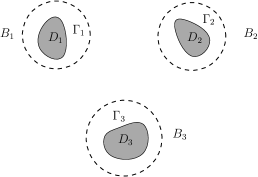
Let us first specify the problem geometry which is shown in Figure 1. Consider the scattering problem for some two-dimensional elastically rigid obstacles, the union of which is represented by a bounded domain $D$ with boundary $\Gamma$. The infinite exterior domain $\mathbb{R}^{2}\setminus\overline{D}$ is assumed to be filled with a homogeneous and isotropic elastic medium. In particular, we assume that the domain $D$ consists of $M$ inclusions $D_{j},j=1,\dots,M$ which are bounded with smooth boundaries $\Gamma_{j}$, i.e., $D=\cup_{j=1}^{M}D_{j}$ and $\Gamma_{j}=\cup_{j=1}^{M}\Gamma_{j}$. Moreover, the obstacles are assumed to be well-separated, i.e., there exist balls $B_{j}$ such that $\overline{D}_{j}\subset B_{j},j=1,\dots,M$ and $B_{i}\cap B_{j}=\emptyset$ for $i\neq j$. Denote by $\nu=(\nu_{1},\nu_{2})$ and $\tau=(\tau_{1},\tau_{2})$ the unit normal and tangential vectors on $\Gamma$, respectively, where $\tau_{1}=-\nu_{2}$ and $\tau_{2}=\nu_{1}$.

Refer to caption
Figure 1. Problem geometry of the elastic scattering by multiple obstacles.

Let the obstacles be illuminated by a time-harmonic plane wave ${\bf u}^{\rm inc}$, which satisfies the two-dimensional Navier equation

$$\mu\Delta{\bf u}^{\rm inc}+(\lambda+\mu)\nabla\nabla\cdot{\bf u}^{\rm inc}+\omega^{2}{\bf u}^{\rm inc}=0\quad\text{in}~{}\mathbb{R}^{2}\setminus\overline{D},$$

where $\omega>0$ is the angular frequency and $\mu,\lambda$ are the Lamé constants satisfying $\mu>0,\lambda+\mu>0$. It can be verified that the incident wave ${\bf u}^{\rm inc}$ has the explicit expression

$${\bf u}^{\rm inc}(x)=de^{{\rm i}k_{p}x\cdot d}\quad\text{or}\quad{\bf u}^{\rm inc}(x)=d^{\perp}e^{{\rm i}k_{s}x\cdot d},$$

where the former is called the compressional plane wave and the latter is referred to as the shear plane wave. Here $d=(\cos\theta,\sin\theta)$ is the unit propagation direction vector, $\theta\in[0,2\pi)$ is the incident angle, $d^{\perp}=(-\sin\theta,\cos\theta)$ is an orthonormal vector of $d$, and

$$k_{p}=\omega/(\lambda+2\mu)^{1/2},\quad k_{s}=\omega/\mu^{1/2}$$

are the compressional wavenumber and the shear wavenumber, respectively. More generally, the incident field can be a linear combination of the compressional and shear plane waves.

The displacement of the total wave field ${\bf u}$ also satisfies the Navier equation

$$\mu\Delta{\bf u}+(\lambda+\mu)\nabla\nabla\cdot{\bf u}+\omega^{2}{\bf u}=0\quad\text{in}~{}\mathbb{R}^{2}\setminus\overline{D}.$$

By assuming that each obstacle is impenetrable and rigid, we have

$${\bf u}=0\quad\text{on}~{}\Gamma.$$

The total field ${\bf u}$ consists of the incident field ${\bf u}^{\rm inc}$ and the scattered field ${\bf v}$:

$${\bf u}={\bf u}^{\rm inc}+{\bf v}.$$

It is easy to verify that the scattered field ${\bf v}$ satisfies the Navier equation

$$\mu\Delta{\bf v}+(\lambda+\mu)\nabla\nabla\cdot{\bf v}+\omega^{2}{\bf v}=0\quad\text{in}~{}\mathbb{R}^{2}\setminus\overline{D}$$ (2.1)

and the boundary condition

$${\bf v}=-{\bf u}^{\rm inc}\quad\text{on}~{}\Gamma.$$ (2.2)

Given a vector function ${\bf w}=(w_{1},w_{2})$ and a scalar function $w$, define the scalar and vector curl operators

$${\rm curl}{\bf w}=\partial_{x_{1}}w_{2}-\partial_{x_{1}}w_{1},\quad{\bf curl}w=(\partial_{x_{2}}w,-\partial_{x_{1}}w).$$

Let ${\bf v}$ be a solution of (2.1). Denote

$${\bf v}_{p}=-\frac{1}{k_{p}^{2}}\nabla\nabla\cdot{\bf v},\quad{\bf v}_{s}=\frac{1}{k_{s}^{2}}{\bf curl}{\rm curl}{\bf v},$$

which are known as the compressional component and the shear component of ${\bf v}$, respectively. Since the scattering problem is imposed in the open domain $\mathbb{R}^{2}\setminus\overline{D}$, the scattered field ${\bf v}$ is required to satisfy the Kupradz–Sommerfeld radiation condition [29], i.e., the components ${\bf v}_{p}$ and ${\bf v}_{s}$ are required to satisfy the Sommerfeld radiation condition:

$$\partial_{\rho}{\bf v}_{p}-{\rm i}k_{p}{\bf v}_{p}=o(\rho^{-1/2}),\quad\partial_{\rho}{\bf v}_{s}-{\rm i}k_{s}{\bf v}_{s}=o(\rho^{-1/2}),\quad\rho=|x|.$$

For any solution ${\bf v}$ of the elastic wave equation (2.1), we introduce the Helmholtz decomposition

$${\bf v}=\nabla\phi+{\bf curl}\psi,$$ (2.3)

where the scalar functions $\phi$ and $\psi$ are called potentials. Substituting (2.3) into (2.1) yields

$$\nabla((\lambda+2\mu)\Delta\phi+\omega^{2}\phi)+{\bf curl}(\mu\Delta\psi+\omega^{2}\psi)=0\quad\text{in}~{}\mathbb{R}^{2}\setminus\overline{D},$$

which is fulfilled if $\phi,\psi$ satisfy the Helmholtz equation

$$\Delta\phi+k_{p}^{2}\phi=0,\quad\Delta\psi+k_{s}^{2}\psi=0\quad\text{in}~{}\mathbb{R}^{2}\setminus\overline{D}.$$

In addition, the potentials $\phi,\psi$ are required to satisfy the Sommerfeld radiation condition

$$\partial_{\rho}\phi-{\rm i}k_{p}\phi=o(\rho^{-1/2}),\quad\partial_{\rho}\psi-{\rm i}k_{s}\psi=o(\rho^{-1/2}).$$

Combining (2.2) and (2.3) yields the boundary condition

$${\bf v}=\nabla\phi+{\bf curl}\psi=-{\bf u}^{\rm inc}\quad\text{on}~{}\Gamma.$$

Taking the dot product of the above equation with $\nu$ and $\tau$, respectively, and noting $\tau_{1}=-\nu_{2},\tau_{2}=\nu_{1}$, we obtain a coupled boundary condition for $\phi_{1},\phi_{2}$ on $\Gamma$:

$$\partial_{\nu}\phi+\partial_{\tau}\psi=f,\quad\partial_{\tau}\phi-\partial_{\nu}\psi=g,$$

where

$$f=-\nu\cdot{\bf u}^{\rm inc},\quad g=-\tau\cdot{\bf u}^{\rm inc}.$$

Hence the obstacle scattering problem for elastic waves can be reduced equivalently to the coupled boundary value problem of the Helmholtz equations:

$$\begin{cases}\Delta\phi+k_{p}^{2}\phi=0,\quad\Delta\psi+k_{s}^{2}\psi=0&\quad\text{in}~{}\mathbb{R}^{2}\setminus\overline{D},\\ \partial_{\nu}\phi+\partial_{\tau}\psi=f,\quad\partial_{\tau}\phi-\partial_{\nu}\psi=g&\quad\text{on}~{}\Gamma,\\ \partial_{\rho}\phi-{\rm i}k_{p}\phi=o(\rho^{-1/2}),\quad\partial_{\rho}\psi-{\rm i}k_{s}\psi=o(\rho^{-1/2})&\quad\text{as}~{}\rho\to\infty.\end{cases}$$ (2.4)

The proof can be found in [21] for the well-posedness of the above scattering problem (2.4) by using the variational approach. In this work, our goal is to develop a new and well-posed boundary integral equation, and propose a fast numerical method to the scattering problem (2.4). Hence we assume that the boundary value problem (2.4) has a unique solution.

Theorem 2.1.

The coupled Helmholtz system (2.4) has at most one solution for $k_{s}>0$ and $k_{p}>0$.

3. Preliminaries of integral operators

Let $\Gamma\subset\mathbb{R}^{2}$ be a smooth closed curve. Consider the integral operators of the form

$\displaystyle F(x)=\int_{\Gamma}K(x,x-y)\phi(y)ds(y)$ (3.1)

and its adjoint with respect to $L^{2}(\Gamma)$

$\displaystyle G(x)=\int_{\Gamma}K(y,y-x)\phi(y)ds(y),$ (3.2)

where $K$ is an integral kernel and $\phi$ is called the density. The following theorem can be found in [24].

Theorem 3.1.

Let $\alpha=(\alpha_{1},\alpha_{2})$ be a multi-index and $\beta$ be a positive integer. Assume that the kernel $K$ in (3.1)–(3.2) is given by

$$K(x,y)=h(x)y^{\alpha}|y|^{2\beta}\ln|y|,$$

where $h(x)$ is a smooth function defined on $\Gamma$. Then the kernel is of class $m=-(|\alpha|+2\beta+1)$. The integral operator in (3.1)–(3.2) associated with the kernel $K$ is continuous from $H^{r}(\Gamma)$ into $H^{r+m}(\Gamma)$ for any real $r$.

Consider the two-dimensional Helmholtz equation

$$\Delta u+k^{2}u=0\quad\text{in}~{}\mathbb{R}^{2},$$ (3.3)

where $k$ is the wavenumber satisfying $\Re(k)>0,\Im(k)\geq 0$. It is known that the Green’s function of (3.3) is

$$\Phi_{k}(x,y)=\frac{\rm i}{4}H^{(1)}_{0}(k|x-y|),$$

where $H^{(1)}_{0}$ is the Hankel function of the first kind with order zero.

Given a bounded domain $D\subset\mathbb{R}^{2}$ with smooth boundary $\Gamma$, let $\nu$ and $\tau$ be the exterior unit normal vector and the unit tangential vector of $\Gamma$, respectively. For $x\notin\Gamma$, define the single and double layer potentials

$\displaystyle\mathcal{S}_{k}\phi(x)$ $\displaystyle=\int_{\Gamma}\Phi_{k}(x,y)\phi(y)ds(y),$
$\displaystyle\mathcal{D}_{k}\phi(x)$ $\displaystyle=\int_{\Gamma}\frac{\partial\Phi_{k}(x,y)}{\partial\nu(y)}\phi(y)ds(y),$

and the tangential boundary layer potential

$$\mathcal{H}_{k}\phi(x)=\int_{\Gamma}\frac{\partial\Phi_{k}(x,y)}{\partial\tau(y)}\phi(y)ds(y).$$

For $k=0$, these potentials denote the layer potentials corresponding to the two-dimensional Laplace equation where the Green’s function is

$$\Phi_{0}(x,y)=-\frac{1}{2\pi}\ln|x-y|.$$

Moreover, these potentials satisfy the well-known jump relations [7]:

$\displaystyle\lim_{x\rightarrow\Gamma^{\pm}}\mathcal{S}_{k}\phi(x)$ $\displaystyle=S_{k}\phi(x)=\int_{\Gamma}\Phi_{k}(x,y)\phi(y)ds(y),$ (3.4a)
$\displaystyle\lim_{x\rightarrow\Gamma^{\pm}}\mathcal{D}_{k}\phi(x)$ $\displaystyle=(\pm\frac{1}{2}+D_{k})\phi(x)=\pm\frac{1}{2}\phi(x)+\int_{\Gamma}\frac{\partial\Phi_{k}(x,y)}{\partial\nu(y)}\phi(y)ds(y),$ (3.4b)
$\displaystyle\lim_{x\rightarrow\Gamma^{\pm}}\frac{\partial\mathcal{S}_{k}\phi(x)}{\partial\nu(x)}$ $\displaystyle=(\mp\frac{1}{2}+D^{\prime}_{k})\phi(x)=\mp\frac{1}{2}\phi(x)+\int_{\Gamma}\frac{\partial\Phi_{k}(x,y)}{\partial\nu(x)}\phi(y)ds(y),$ (3.4c)
$\displaystyle\lim_{x\rightarrow\Gamma^{\pm}}\mathcal{H}_{k}\phi(x)$ $\displaystyle=H_{k}\phi(x)=\int_{\Gamma}\frac{\partial\Phi_{k}(x,y)}{\partial\tau(y)}\phi(y)ds(y),$ (3.4d)

where the plus sign means that $x$ approaches $\Gamma$ from the exterior and the minus sign stands for that $x$ approaches $\Gamma$ from the interior. The boundary operators $D_{k}$, $D^{\prime}_{k}$, and $H_{k}$ are defined in the sense of Cauchy principal value. In $L^{2}(\Gamma)$, $S_{k}$ is self-adjoint, i.e., $S_{k}=S_{k}^{\prime}$, and $D^{\prime}_{k}$ is the adjoint of $D_{k}$. The adjoint of $H_{k}$ is given by

$$H^{\prime}_{k}\phi(x)=\frac{\partial S_{k}\phi(x)}{\partial\tau(x)}=\int_{\Gamma}\frac{\partial\Phi_{k}(x,y)}{\partial\tau(x)}\phi(y)ds(y).$$

For further investigation, it is indispensable to study the regularity of all these boundary operators. We begin with the asymptotic form of the Green function $\Phi_{k}(x,y)$ which can be found in [25].

Lemma 3.2.

When $k>0$, the Green’s function $\Phi_{k}$ has the expansion

$$\Phi_{k}(x,y)=\Phi_{0}(x,y)-\frac{k^{2}|x-y|^{2}}{4}\Phi_{0}(x,y)+|x-y|^{4}p_{1}(|x-y|^{2})\Phi_{0}(x,y)+p_{2}(|x-y|^{2}),$$

where $p_{1}(x)$ and $p_{2}(x)$ are analytic functions.

Combining Theorem 3.1 and Lemma 3.2, we obtain several useful properties for the integral operators. The following results are related to the regularity of boundary operators $D_{k}$, $H_{k}$ and their adjoint.

Corollary 3.3.

The following operators are bounded:

$\displaystyle D_{0},D^{\prime}_{0}:H^{r}(\Gamma)\rightarrow H^{r+s}(\Gamma),$
$\displaystyle H_{0},H^{\prime}_{0}:H^{r}(\Gamma)\rightarrow H^{r}(\Gamma),$
$\displaystyle D_{k},D^{\prime}_{k}:H^{r}(\Gamma)\rightarrow H^{r+3}(\Gamma),$
$\displaystyle H_{k},H^{\prime}_{k}:H^{r}(\Gamma)\rightarrow H^{r}(\Gamma),$

where $r$ is an arbitrary real number and $s$ is an arbitrary positive real number.

Proof.

We only show the proof of for the integral operators $D_{k}$ and $D_{k}^{\prime}$, since the results are standard and can be found in [7] for other integral operators. It follows from Lemma 3.2 that the kernel $D_{k}$ satisfies

$\displaystyle\frac{\partial\Phi_{k}(x,y)}{\partial\nu(y)}$ $\displaystyle=\frac{\partial\Phi_{0}(x,y)}{\partial\nu(y)}-\frac{|k|^{2}}{4}\frac{\partial(|x-y|^{2}\Phi_{0}(x,y))}{\partial\nu(y)}+O\bigg{(}\frac{\partial(|x-y|^{4}\Phi_{0}(x,y))}{\partial\nu(y)}\bigg{)}$
$\displaystyle=K_{0}(x,y)-\frac{|k|^{2}}{4}K_{1}(x,y)+K_{2}(x,y),$

where $K_{0}$ is the kernel for the integral operator $D_{0}$ and is of class $-\infty$, and $K_{2}$ is of class at most $-4$ by Theorem 3.1. A simple calculation yields

$\displaystyle K_{1}(x,y)$ $\displaystyle=\frac{\partial(|x-y|^{2}\Phi_{0}(x,y))}{\partial\nu(y)}$
$\displaystyle=\frac{\partial|x-y|^{2}}{\partial\nu(y)}\Phi_{0}(x,y)+\frac{\partial\Phi_{0}(x,y)}{\partial\nu(y)}|x-y|^{2}$
$\displaystyle=-2(\nu(y)\cdot(x-y))\Phi_{0}(x,y)+K_{0}(x,y)|x-y|^{2}.$

For a smooth curve $\Gamma$, it is shown in [7] that

$$\nu(y)\cdot(x-y)=O(|x-y|^{2}).$$

Hence it follows from Theorem 3.1 that $K_{1}$ is a kernel of class $-3$ and $D_{k}$ is a bounded operator from $H^{r}(\Gamma)$ to $H^{r+3}(\Gamma)$. Similarly we can show that the kernel of $D^{\prime}_{k}$ is also of class $-3$, which completes the proof. ∎

The following results are related to the properties of difference of boundary operators. The proof is similar to that for Corollary 3.3, so we omit it.

Corollary 3.4.

The following mappings are bounded:

$\displaystyle D_{k}-D_{0},D^{\prime}_{k}-D^{\prime}_{0}:H^{r}(\Gamma)\rightarrow H^{r+3}(\Gamma),$
$\displaystyle H_{k}-H_{0},H^{\prime}_{k}-H_{0}:H^{r}(\Gamma)\rightarrow H^{r+2}(\Gamma),$

where $r$ is an arbitrary real number.

The next lemma follows from the property of Cauchy integrals [17].

Lemma 3.5.

Let $\Gamma\subset\mathbb{R}^{2}$ be a smooth curve. Then

$\displaystyle D_{0}^{2}-H_{0}^{2}=\frac{I}{4},\quad H_{0}D_{0}=-D_{0}H_{0},\quad{D^{\prime}_{0}}^{2}-{H^{\prime}_{0}}^{2}=\frac{I}{4},\quad{H^{\prime}_{0}}{D^{\prime}_{0}}=-D^{\prime}_{0}H^{\prime}_{0},$

where $I$ is the identity operator.

In this paper, we mainly focus on functions in $H^{1/2}(\Gamma)$ and $H^{-1/2}(\Gamma)$, which are the trace space of $H^{1}(D)$ and $L^{2}(D)$, respectively. We also denote the vector function space with each component in $H^{1/2}(\Gamma)$ by $H^{1/2}(\Gamma)^{2}$. Similar notation applies to $H^{s}(\Gamma)$ for any real $s$. It is well known that the two dimensional single layer boundary operator $S_{0}$, which is bounded from $H^{s}(\Gamma)$ to $H^{s+1}(\Gamma)$, is not invertible in general. However, we have the following result which can be found in [17]:

Lemma 3.6.

There exists a constant $c>0$, which only depends on the curve $\Gamma$, such that the operator $\overline{S}_{0}$, defined by

$$(\overline{S}_{0}\phi)(x)=\int_{\Gamma}(\Phi_{0}(x,y)+c)\phi(y)ds(y)=S_{0}\phi(x)+\int_{\Gamma}c\phi(y)ds(y),$$

is invertible from $H^{s}(\Gamma)$ to $H^{s+1}(\Gamma)$ for any real $s$.

To this end, we denote the operator

$\displaystyle\overline{\mathbf{S}}_{0}\overline{\mathbf{S}}_{0}=\begin{bmatrix}\overline{S}_{0}\overline{S}_{0}&0\\ 0&\overline{S}_{0}\overline{S}_{0}\end{bmatrix}$

for a vector function ${\bf w}=(w_{1},w_{2})\in H^{s}(\Gamma)^{2}$ by $\overline{\mathbf{S}}_{0}\overline{\mathbf{S}}_{0}$. By Lemma 3.6, the operator $\overline{\mathbf{S}}_{0}\overline{\mathbf{S}}_{0}$ is invertible from $H^{s}(\Gamma)^{2}$ to $H^{s+2}(\Gamma)^{2}$.

4. Boundary integral equations

In this section, we derive boundary integral equations for the scattering problem (2.4) and show the well-posedness of the proposed boundary integral equations. For clarity, we restrict our discussion to the scattering of a single particle, which is still denoted by $D$ with boundary $\Gamma$.

Define two single layer potentials corresponding to the compressional and shear wavenumbers:

$$\phi(x)=\mathcal{S}_{k_{p}}\alpha(x),\quad\psi(x)=\mathcal{S}_{k_{s}}\beta(x),$$

where $(\alpha(x),\beta(x))\in H^{-1/2}(\Gamma)^{2}$ are densities. Using the boundary condition (2.2) and the jump relations (3.4), we obtain the integral equation

$\displaystyle A\begin{bmatrix}\alpha(x)\\ \beta(x)\end{bmatrix}=\begin{bmatrix}-\frac{I}{2}+D^{\prime}_{k_{p}}&H^{\prime}_{k_{s}}\\ H^{\prime}_{k_{p}}&\frac{I}{2}-D^{\prime}_{k_{s}}\end{bmatrix}\begin{bmatrix}\alpha(x)\\ \beta(x)\end{bmatrix}=\begin{bmatrix}f(x)\\ g(x)\end{bmatrix}.$ (4.1)

where $I$ is the identity operator. We first state the following existence result for equation (4.1).

Theorem 4.1.

Assume that neither $k_{s}$ or $k_{p}$ is the eigenvalue of the interior Dirichlet problem for the Helmholtz equation in $D$. Then the integral equation (4.1) has a unique solution in $H^{-1/2}(\Gamma)^{2}$.

Remark 4.2.

It is easy to see that $A=A_{0}+K$, where

$\displaystyle A_{0}=\begin{bmatrix}-\frac{I}{2}&H^{\prime}_{0}\\ H^{\prime}_{0}&\frac{I}{2}\end{bmatrix}$ (4.2)

is bounded in $H^{-1/2}(\Gamma)^{2}$ and $K$ is a compact operator in $H^{-1/2}(\Gamma)^{2}$. If $A_{0}$ is invertible, Fredholm alternative can be directly applied to show the invertibility of $A$. However, $A_{0}$ is degenerated in the sense that

$\displaystyle A^{2}_{0}=\begin{bmatrix}{D^{\prime}}^{2}_{0}&0\\ 0&{D^{\prime}}^{2}_{0}\end{bmatrix},$ (4.3)

where $D^{\prime}_{0}$ is a smooth operator by Corollary 3.3.

The existence result also holds for the integral representation by using double layer potentials

$$\phi(x)=\mathcal{D}_{k_{p}}\alpha(x),\quad\psi(x)=\mathcal{D}_{k_{s}}\beta(x).$$

Using the jump relations (3.4), we obtain the integral equation

$\displaystyle M\begin{bmatrix}\alpha(x)\\ \beta(x)\end{bmatrix}=\begin{bmatrix}f(x)\\ g(x)\end{bmatrix},$ (4.4)

where the coefficient matrix

$$M=\begin{bmatrix}T_{k_{p}}&\frac{1}{2}\partial_{\tau}+\partial_{\tau}D_{k_{s}}\\ \frac{1}{2}\partial_{\tau}+\partial_{\tau}D_{k_{p}}&-T_{k_{s}}\end{bmatrix}.$$

and $T_{k}=\partial_{\nu}D_{k}$. It holds the following existence result.

Theorem 4.3.

If neither $k_{s}$ or $k_{p}$ is the eigenvalue of the interior Neumann problem for the Helmholtz equation in $D$, the integral equation (4.4) has a unique solution in $H^{1/2}(\Gamma)^{2}$.

To remove the assumption of Theorem 4.1 or 4.3, we propose a combined double and single layer representation to obtain a uniquely solvable integral system for any $k_{s}$ and $k_{p}$. Consider the combined layer potentials

$$\phi(x)=(\mathcal{D}_{k_{p}}-{\rm i}\mathcal{S}_{k_{p}})\alpha(x),\quad\psi(x)=(\mathcal{D}_{k_{s}}-{\rm i}\mathcal{S}_{k_{s}})\beta(x),$$

which results in a combined integral equation

$\displaystyle(M-{\rm i}A)\begin{bmatrix}\alpha(x)\\ \beta(x)\end{bmatrix}$ $\displaystyle=\left(\begin{bmatrix}T_{k_{p}}&\frac{1}{2}\partial_{\tau}+\partial_{\tau}D_{k_{s}}\\ \frac{1}{2}\partial_{\tau}+\partial_{\tau}D_{k_{p}}&-T_{k_{s}}\end{bmatrix}-{\rm i}\begin{bmatrix}-\frac{1}{2}+D^{\prime}_{k_{p}}&H^{\prime}_{k_{s}}\\ H^{\prime}_{k_{p}}&\frac{1}{2}-D^{\prime}_{k_{s}}\end{bmatrix}\right)\begin{bmatrix}\alpha(x)\\ \beta(x)\end{bmatrix}$
$\displaystyle=\begin{bmatrix}f(x)\\ g(x)\end{bmatrix}.$ (4.5)

We have the following existence result.

Theorem 4.4.

For any $k_{p}>0$ and $k_{s}>0$, the integral equation (4) admits a unique solution in $H^{1/2}(\Gamma)^{2}$.

In what follows, we discuss the proofs of Theorems 4.1, 4.3 and 4.4 in details.

4.1. Proof of Theorem 4.1

To construct an appropriate regularizer for the operator $A$, we consider the interior problem of the coupled Helmholtz system

$\displaystyle\begin{cases}\Delta\phi+k_{p}^{2}\phi=0,\quad\Delta\psi+k_{s}^{2}\psi=0&\quad\text{in}~{}D,\\ -\partial_{\nu}\phi+\partial_{\tau}\psi=f,\quad\partial_{\tau}\phi+\partial_{\nu}\psi=g&\quad\text{on}~{}\Gamma.\end{cases}$ (4.6)

Assume the solutions $\phi$ and $\psi$ have the integral representations

$$\phi=S_{k_{p}}\alpha(x),\quad\psi=S_{k_{s}}\beta(x).$$

Using the boundary condition, we obtain the integral equation

$$B\begin{bmatrix}\alpha\\ \beta\end{bmatrix}=\begin{bmatrix}f\\ g\end{bmatrix},\mbox{ where }B=\begin{bmatrix}-\frac{I}{2}-D^{\prime}_{k_{p}}&H^{\prime}_{k_{s}}\\ H^{\prime}_{k_{p}}&\frac{I}{2}+D^{\prime}_{k_{s}}\end{bmatrix}.$$

To prove Theorem 4.1, we also need to derive the adjoint operator of $A$ in $L^{2}(\Gamma)^{2}$. By applying Green’s identity to equation (4.6), it holds for $x\in\Gamma^{-}$ that

$\displaystyle\left(\frac{I}{2}+D_{k_{p}}\right)\phi-S_{k_{p}}\partial_{\nu}\phi$ $\displaystyle=\phi,$
$\displaystyle\left(\frac{I}{2}+D_{k_{s}}\right)\psi-S_{k_{s}}\partial_{\nu}\psi$ $\displaystyle=\psi.$

It follows from the boundary condition in equation (4.6) that we have

$\displaystyle\left(-\frac{I}{2}+D_{k_{p}}\right)\phi-S_{k_{p}}\partial_{\tau}\psi$ $\displaystyle=-S_{k_{p}}f,$
$\displaystyle\left(-\frac{I}{2}+D_{k_{s}}\right)\psi+S_{k_{s}}\partial_{\tau}\phi$ $\displaystyle=S_{k_{s}}g.$

Noting $H_{k}\phi=-S_{k}\partial_{\tau}\phi$, we obtain

$$A^{\prime}\begin{bmatrix}\phi\\ \psi\end{bmatrix}=\begin{bmatrix}-\frac{I}{2}+D_{k_{p}}&H_{k_{p}}\\ H_{k_{s}}&\frac{I}{2}-D_{k_{s}}\end{bmatrix}\begin{bmatrix}\phi\\ \psi\end{bmatrix}=\begin{bmatrix}-S_{k_{p}}f\\ -S_{k_{s}}g\end{bmatrix}.$$

It is easy to check that the operator $A^{\prime}$ is the adjoint of the operator $A$ with respect to the bilinear form in $L^{2}(\Gamma)^{2}$ given by

$$\langle{\bf u},{\bf v}\rangle=\int_{\Gamma}\big{(}u_{1}v_{1}+u_{2}v_{2}\big{)}ds.$$

where ${\bf u}=(u_{1},u_{2})$ and ${\bf v}=(v_{1},v_{2})$.

Theorem 4.5.

For any vector function ${\bf f}\in H^{-1/2}(\Gamma)^{2}$, the operators $A,B$ satisfy

$\displaystyle(AB){\bf f}=\left(-\frac{(k^{2}_{s}+k^{2}_{p})}{2}\overline{\mathbf{S}}_{0}\overline{\mathbf{S}}_{0}+K_{1}\right){\bf f},$
$\displaystyle(BA){\bf f}=\left(-\frac{(k^{2}_{s}+k^{2}_{p})}{2}\overline{\mathbf{S}}_{0}\overline{\mathbf{S}}_{0}+K_{2}\right){\bf f},$

where $K_{1},K_{2}$ are compact operators from $H^{-1/2}(\Gamma)^{2}$ to $H^{3/2}(\Gamma)^{2}$.

Proof.

It follows from a straightforward calculation that

$\displaystyle AB$ $\displaystyle=\begin{bmatrix}-\frac{I}{2}+D^{\prime}_{k_{p}}&H^{\prime}_{k_{s}}\\ H^{\prime}_{k_{p}}&\frac{I}{2}-D^{\prime}_{k_{s}}\end{bmatrix}\begin{bmatrix}-\frac{I}{2}-D^{\prime}_{k_{p}}&H^{\prime}_{k_{s}}\\ H^{\prime}_{k_{p}}&\frac{I}{2}+D^{\prime}_{k_{s}}\end{bmatrix}$
$\displaystyle=\begin{bmatrix}\frac{I}{4}-(D^{\prime}_{k_{p}})^{2}+H^{\prime}_{k_{s}}H^{\prime}_{k_{p}}&D^{\prime}_{k_{p}}H^{\prime}_{k_{s}}+H^{\prime}_{k_{s}}D^{\prime}_{k_{s}}\\ -D^{\prime}_{k_{s}}H^{\prime}_{k_{p}}-H^{\prime}_{k_{p}}D^{\prime}_{k_{p}}&\frac{I}{4}-(D^{\prime}_{k_{s}})^{2}+H^{\prime}_{k_{p}}H^{\prime}_{k_{s}}\end{bmatrix}.$

We first look at the off diagonal elements. It can be verified that

$\displaystyle D^{\prime}_{k_{p}}H^{\prime}_{k_{s}}+H^{\prime}_{k_{s}}D^{\prime}_{k_{s}}=$ $\displaystyle(D^{\prime}_{k_{p}}-D^{\prime}_{0})H^{\prime}_{0}+D^{\prime}_{k_{p}}(H^{\prime}_{k_{s}}-H^{\prime}_{0})$
$\displaystyle\quad+H^{\prime}_{k_{s}}(D^{\prime}_{k_{s}}-D^{\prime}_{0})+(H^{\prime}_{k_{s}}-H^{\prime}_{0})D^{\prime}_{0},$

where $D^{\prime}_{0}H^{\prime}_{0}+H^{\prime}_{0}D^{\prime}_{0}$ vanishes due to Lemma 3.5. It follows from Corollaries 3.3 and 3.4 that $(D^{\prime}_{k_{p}}-D^{\prime}_{0})H^{\prime}_{0},H^{\prime}_{k_{s}}(D^{\prime}_{k_{s}}-D^{\prime}_{0})$ are bounded operators from $H^{-1/2}(\Gamma)$ to $H^{-1/2+3}(\Gamma)$ and $D^{\prime}_{k_{p}}(H^{\prime}_{k_{s}}-H^{\prime}_{0}),(H^{\prime}_{k_{s}}-H^{\prime}_{0})D^{\prime}_{0}$ are bounded operators from $H^{-1/2}(\Gamma)$ to $H^{-1/2+5}(\Gamma)$. Therefore, $D^{\prime}_{k_{p}}H^{\prime}_{k_{s}}+H^{\prime}_{k_{s}}D^{\prime}_{k_{s}}$ is a compact operator from $H^{-1/2}(\Gamma)$ to $H^{3/2}(\Gamma)$. Similarly, we can show that $-D^{\prime}_{k_{s}}H^{\prime}_{k_{p}}-H^{\prime}_{k_{p}}D^{\prime}_{k_{p}}$ is also a compact operator from $H^{-1/2}(\Gamma)$ to $H^{3/2}(\Gamma)$.

Next we check the diagonal elements. Using Lemma 3.5, we obtain

$\displaystyle\frac{I}{4}-(D^{\prime}_{k_{p}})^{2}+H^{\prime}_{k_{s}}H^{\prime}_{k_{p}}=$ $\displaystyle(H^{\prime}_{k_{s}}-H^{\prime}_{0})H^{\prime}_{0}+H^{\prime}_{k_{s}}(H^{\prime}_{k_{p}}-H^{\prime}_{0})$
$\displaystyle\quad-(D^{\prime}_{k_{p}})^{2}+(D^{\prime}_{0})^{2},$
$\displaystyle\frac{I}{4}-(D^{\prime}_{k_{s}})^{2}+H^{\prime}_{k_{p}}H^{\prime}_{k_{s}}=$ $\displaystyle(H^{\prime}_{k_{p}}-H^{\prime}_{0})H^{\prime}_{0}+H^{\prime}_{k_{p}}(H^{\prime}_{k_{s}}-H^{\prime}_{0})$
$\displaystyle\quad-(D^{\prime}_{k_{s}})^{2}+(D^{\prime}_{0})^{2}.$

From Corollaries 3.3 and 3.4, the operators $(D^{\prime}_{k_{p}})^{2}$, $(D^{\prime}_{0})^{2}$ are bounded from $H^{-1/2}(\Gamma)$ to $H^{-1/2+6}(\Gamma)$. Hence they are both compact from $H^{-1/2}(\Gamma)$ to $H^{3/2}(\Gamma)$. Consider the operator

$$(H^{\prime}_{k_{s}}-H^{\prime}_{0})H^{\prime}_{0}+H^{\prime}_{k_{s}}(H^{\prime}_{k_{p}}-H^{\prime}_{0}).$$ (4.7)

Clearly, it is bounded from $H^{-1/2}(\Gamma)$ to $H^{3/2}(\Gamma)$. Using the asymptotic form in Lemma 3.2, we have the following decomposition

$\displaystyle(H^{\prime}_{k_{s}}-H^{\prime}_{0})H^{\prime}_{0}\phi(x)$ $\displaystyle=-\frac{\partial}{\partial\tau(x)}\int_{\Gamma}\frac{|k_{s}(x-y)|^{2}}{4}\Phi_{0}(x,y)$
$\displaystyle\qquad\times\frac{\partial}{\partial\tau(y)}\int_{\Gamma}\Phi_{0}(y,z)\phi(z)ds(z)ds(y)+K_{1}\phi(x),$
$\displaystyle H^{\prime}_{k_{s}}(H^{\prime}_{k_{p}}-H^{\prime}_{0})\phi(x)$ $\displaystyle=-\frac{\partial}{\partial\tau(x)}\int_{\Gamma}\Phi_{0}(x,y)$
$\displaystyle\qquad\times\frac{\partial}{\partial\tau(y)}\int_{\Gamma}\frac{|k_{p}(y-z)|^{2}}{4}\Phi_{0}(y,z)\phi(z)ds(z)ds(y)+K_{2}\phi(x),$

where $K_{1}$ and $K_{2}$ are compact operators from $H^{-1/2}(\Gamma)$ to $H^{3/2}(\Gamma)$. For the first operator in the right hand side of $(H^{\prime}_{k_{s}}-H^{\prime}_{0})H^{\prime}_{0}$, we note

$\displaystyle-\frac{\partial}{\partial\tau(x)}\int_{\Gamma}\frac{|k_{s}(x-y)|^{2}}{4}\Phi_{0}(x,y)\frac{\partial}{\partial\tau(y)}\int_{\Gamma}\Phi_{0}(y,z)\phi(z)ds(z)ds(y)$
$\displaystyle=\int_{\Gamma}\frac{\partial}{\partial\tau(x)}\bigg{(}\frac{\partial}{\partial\tau(y)}\frac{|k_{s}(x-y)|^{2}}{4}\Phi_{0}(x,y)\bigg{)}\int_{\Gamma}\Phi_{0}(y,z)\phi(z)ds(z)ds(y)$
$\displaystyle=\int_{\Gamma}\bigg{(}\frac{\partial}{\partial\tau(x)}+\frac{\partial}{\partial\tau(y)}\bigg{)}\bigg{(}\frac{\partial}{\partial\tau(y)}\frac{|k_{s}(x-y)|^{2}}{4}\Phi_{0}(x,y)\bigg{)}\int_{\Gamma}\Phi_{0}(y,z)\phi(z)ds(z)ds(y)$
$\displaystyle\qquad-\int_{\Gamma}\frac{\partial}{\partial\tau(y)}\bigg{(}\frac{\partial}{\partial\tau(y)}\frac{|k_{s}(x-y)|^{2}}{4}\Phi_{0}(x,y)\bigg{)}\int_{\Gamma}\Phi_{0}(y,z)\phi(z)ds(z)ds(y)$
$\displaystyle=M\phi(x)+N\phi(x),$

where $M$ denotes the first operator and $N$ denotes the second one.

We show that $M$ is a compact operator from $H^{-1/2}(\Gamma)$ to $H^{3/2}(\Gamma)$. In fact, it holds

$\displaystyle\bigg{(}\frac{\partial}{\partial\tau(x)}+\frac{\partial}{\partial\tau(y)}\bigg{)}\bigg{(}\frac{\partial}{\partial\tau(y)}\frac{|k_{s}(x-y)|^{2}}{4}\Phi_{0}(x,y)\bigg{)}$
$\displaystyle=-\frac{k_{s}^{2}}{4\pi}(1-\tau(x)\tau(y))\ln(|x-y|)+O((x-y)\ln(|x-y|))$
$\displaystyle=O((x-y)\ln(|x-y|)).$

By Theorem 3.1, $M$ is bounded from $H^{-1/2}(\Gamma)$ to $H^{5/2}(\Gamma)$ which implies that $M$ is compact from $H^{-1/2}(\Gamma)$ to $H^{3/2}(\Gamma)$. For the operator $N$, it is clear to note that

$\displaystyle-\frac{\partial}{\partial\tau(y)}\bigg{(}\frac{\partial}{\partial\tau(y)}\frac{|k_{s}(x-y)|^{2}}{4}\Phi_{0}(x,y)\bigg{)}$
$\displaystyle=-\frac{k_{s}^{2}}{2}\Phi_{0}(x-y)+O((x-y)\ln(|x-y|)).$

Therefore,

$\displaystyle N\phi(x)=-\frac{k_{s}^{2}}{2}S_{0}S_{0}\phi(x)+K\phi(x),$ (4.8)

where $K$ is compact from $H^{-1/2}(\Gamma)$ to $H^{3/2}(\Gamma)$. Similarly, the following property can be shown for the operator $H^{\prime}_{k_{s}}(H^{\prime}_{k_{p}}-H^{\prime}_{0})$

$\displaystyle\left(H^{\prime}_{k_{s}}(H^{\prime}_{k_{p}}-H^{\prime}_{0})\right)\phi(x)=-\frac{k_{p}^{2}}{2}S_{0}S_{0}\phi(x)+K\phi(x)$

Combining (4.7)–(4.8), we obtain

$\displaystyle\left(\frac{I}{4}-(D^{\prime}_{k_{p}})^{2}+H^{\prime}_{k_{s}}H^{\prime}_{k_{p}}\right)\phi=\left(-\frac{(k_{s}^{2}+k_{p}^{2})}{2}S_{0}S_{0}+K\right)\phi,$

where $K$ is a compact operator from $H^{-1/2}(\Gamma)$ to $H^{3/2}(\Gamma)$. Following the same argument, we can show

$\displaystyle\left(\frac{I}{4}-(D^{\prime}_{k_{s}})^{2}+H^{\prime}_{k_{p}}H^{\prime}_{k_{s}}\right)\phi=\left(-\frac{(k_{s}^{2}+k_{p}^{2})}{2}S_{0}S_{0}+K\right)\phi,$

which proves the first part of the theorem since $\overline{S}_{0}$ and $S_{0}$ only differ by a smooth operator.

For the second part, we have from straightforward calculations that

$\displaystyle BA$ $\displaystyle=\begin{bmatrix}-\frac{I}{2}-D^{\prime}_{k_{p}}&H^{\prime}_{k_{s}}\\ H^{\prime}_{k_{p}}&\frac{I}{2}+D^{\prime}_{k_{s}}\end{bmatrix}\begin{bmatrix}-\frac{I}{2}+D^{\prime}_{k_{p}}&H^{\prime}_{k_{s}}\\ H^{\prime}_{k_{p}}&\frac{I}{2}-D^{\prime}_{k_{s}}\end{bmatrix}$
$\displaystyle=\begin{bmatrix}\frac{I}{4}-(D^{\prime}_{k_{p}})^{2}+H^{\prime}_{k_{p}}H^{\prime}_{k_{s}}&-D^{\prime}_{k_{p}}H^{\prime}_{k_{s}}-H^{\prime}_{k_{s}}D^{\prime}_{k_{s}}\\ D^{\prime}_{k_{s}}H^{\prime}_{k_{p}}+H^{\prime}_{k_{p}}D^{\prime}_{k_{p}}&\frac{I}{4}-(D^{\prime}_{k_{s}})^{2}+H^{\prime}_{k_{p}}H^{\prime}_{k_{s}}\end{bmatrix}.$

The rest of the proof is the same as the first part and is omitted here. ∎

Next we consider the adjoint operator $A^{\prime}$ and introduce the operator

$\displaystyle B^{\prime}=\begin{bmatrix}-\frac{I}{2}-D_{k_{p}}&H_{k_{p}}\\ H_{k_{s}}&\frac{I}{2}+D_{k_{s}}\end{bmatrix},$

which is the adjoint of operator $B$ in $L^{2}(\Gamma)^{2}$. Following exactly the same argument, we have the following result.

Theorem 4.6.

For any vector function ${\bf f}\in H^{1/2}(\Gamma)^{2}$, the operators $A^{\prime},B^{\prime}$ satisfy

$\displaystyle(A^{\prime}B^{\prime}){\bf f}=\left(-\frac{(k^{2}_{s}+k^{2}_{p})}{2}\overline{\mathbf{S}}_{0}\overline{\mathbf{S}}_{0}+K_{1}\right){\bf f}$
$\displaystyle(B^{\prime}A^{\prime}){\bf f}=\left(-\frac{(k^{2}_{s}+k^{2}_{p})}{2}\overline{\mathbf{S}}_{0}\overline{\mathbf{S}}_{0}+K_{2}\right){\bf f}$

where $K_{1},K_{2}$ are compact operators from $H^{1/2}(\Gamma)^{2}$ to $H^{5/2}(\Gamma)^{2}$.

Since $\overline{\mathbf{S}}_{0}\overline{\mathbf{S}}_{0}$ is invertible from $H^{s}(\Gamma)^{2}$ to $H^{s+2}(\Gamma)^{2}$ with $s\in\mathbb{R}$, by the Fredholm alternative, the operators $A$ and $A^{\prime}$ have finite dimensional null spaces and their ranges are given by

$\displaystyle{\rm Ran}(A)$ $\displaystyle=\{{\bf f}\in H^{-1/2}(\Gamma)^{2}:\langle{\bf f},{\bf g}\rangle=0,\,{\bf g}\in{\rm Ker}(A^{\prime})\},$
$\displaystyle{\rm Ran}(A^{\prime})$ $\displaystyle=\{{\bf f}\in H^{1/2}(\Gamma)^{2}:\langle{\bf f},{\bf h}\rangle=0,\,{\bf h}\in{\rm Ker}(A)\}.$

The kernel of $A$ and $A^{\prime}$ are given in the following theorem.

Theorem 4.7.

If neither $k_{s}$ or $k_{p}$ is the eigenvalue of the interior Dirichlet problem for the Helmholtz equation in $D$, then ${\rm Ker}(A)={\rm Ker}(A^{\prime})=\{0\}$.

Proof.

Assume $(\alpha(x),\beta(x))\in H^{-1/2}(\Gamma)^{2}$ satisfies

$$A\begin{bmatrix}\alpha\\ \beta\end{bmatrix}=\begin{bmatrix}0\\ 0\end{bmatrix}.$$

Let

$$\phi(x)=\mathcal{S}_{k_{p}}\alpha(x),\quad\psi(x)=\mathcal{S}_{k_{s}}\beta(x),\quad x\in\mathbb{R}^{2}\setminus\Gamma.$$

Then $(\phi,\psi)$ satisfies (2.4) with $f=0,g=0.$ By the uniqueness result in Theorem 2.1, it holds

$$\phi(x)=\psi(x)=0,\quad x\in\mathbb{R}^{2}\setminus\overline{D}.$$

It follows from the continuity of single layer potential that $\phi(x)=\psi(x)=0$ for $x\in\Gamma^{-}$. Since neither $k_{s}$ or $k_{p}$ is the eigenvalue of the interior Dirichlet problem in $D$, we have $\phi(x)=\psi(x)=0$ for $x\in D$. Using the jump relation of double layer potential, we obtain $\alpha(x)=\beta(x)=0$, which implies ${\rm Ker}(A)=\{0\}$.

Now assume $(\alpha(x),\beta(x))\in{\rm Ker}(A^{\prime})$. Let $x\in\mathbb{R}^{2}\setminus\Gamma$ and consider

$\displaystyle\phi(x)$ $\displaystyle=\mathcal{D}_{k_{p}}\alpha(x)-\mathcal{S}_{k_{p}}\partial_{\tau}\beta(x),$
$\displaystyle\psi(x)$ $\displaystyle=\mathcal{D}_{k_{s}}\beta(x)+\mathcal{S}_{k_{s}}\partial_{\tau}\alpha(x).$

Since $\phi(x)=\psi(x)=0$ when $x$ approaches $\Gamma$ from the interior, by assumption, it holds $\phi(x)=\psi(x)=0$ for $x\in D$. By Green’s theorem, when $x$ approaches $\Gamma$ from the exterior, i.e., $x\rightarrow\Gamma^{+}$, we have

$\displaystyle\phi(x)=\alpha(x),$ $\displaystyle\quad\psi(x)=\beta(x),$ (4.9a)
$\displaystyle\partial_{\nu}\phi(x)=\partial_{\tau}\beta(x),$ $\displaystyle\quad\partial_{\nu}\psi(x)=-\partial_{\tau}\alpha(x),$ (4.9b)

which shows that $\phi$ and $\psi$ satisfies (2.4) with $f=g=0$. Therefore, by the uniqueness of the scattering problem, $\phi(x)=\psi(x)=0$ in $\mathbb{R}^{2}\setminus\overline{D}$. Following (4.9) it yields that $\alpha(x)=\beta(x)=0$, which completes the proof. ∎

The well-posedness of the integral equation (4.1) follows immediately from the Fredholm alternative, which completes the proof of Theorem 4.1.

Remark 4.8.

In practice, the assumption of Theorem 4.1 may be violated for a given domain $D$. Besides using the combined layer representation as given in Theorem 4.4, this issue can also be resolved based on a modified single layer representation when domain $D$ is simply connected and $0\in D$. Following the idea in [7], we can modify the integral representation to

$\displaystyle\phi(x)=\mathcal{S}_{k_{p}}\alpha(x)+\sum_{n=0}^{\infty}a_{n}H^{(1)}_{n}(k_{p}|x|)e^{{\rm i}n\frac{x}{|x|}}\int_{\Gamma}H^{(1)}_{n}(k_{p}|y|)e^{{\rm i}n\frac{y}{|y|}}\alpha(y)ds(y),$ (4.10a)
$\displaystyle\psi(x)=\mathcal{S}_{k_{s}}\beta(x)+\sum_{n=0}^{\infty}b_{n}H^{(1)}_{n}(k_{s}|x|)e^{{\rm i}n\frac{x}{|x|}}\int_{\Gamma}H^{(1)}_{n}(k_{s}|y|)e^{{\rm i}n\frac{y}{|y|}}\beta(y)ds(y),$ (4.10b)

where $\hat{x}=x/|x|,\hat{y}=y/|y|$ and $H_{n}^{(1)}$ is the Hankel function of the first kind with order $n$. Under some appropriate assumptions on $\{a_{n}\}$ and $\{b_{n}\}$, it can be shown the the representation (4.10) is free of resonance. Readers are referred to [7] for more details.

4.2. Proof of Theorem 4.3

Introduce the operator

$\displaystyle N=\begin{bmatrix}S_{k_{p}}&0\\ 0&S_{k_{s}}\end{bmatrix}\begin{bmatrix}T_{k_{p}}&\frac{1}{2}\partial_{\tau}-\partial_{\tau}D_{k_{s}}\\ \frac{1}{2}\partial_{\tau}-\partial_{\tau}D_{k_{p}}&-T_{k_{s}}\end{bmatrix}\begin{bmatrix}S_{k_{p}}&0\\ 0&S_{k_{s}}\end{bmatrix}.$

We show that $N$ is a regularizer of $M$ in (4.4). Let us begin with the Calderon identities which can be found in [24].

Lemma 4.9.

Let $I$ be the identity operator and $k$ be the wavenumber with $k>0$. For a smooth closed curve $\Gamma\subset\mathbb{R}^{2}$, it holds that

$$D^{2}_{k}-S_{k}T_{k}=\frac{I}{4},\quad D^{\prime 2}_{k}-T_{k}S_{k}=\frac{I}{4}.$$

Analogous to Theorem 4.5, we have the following result for operators $M$ and $N$.

Theorem 4.10.

For any vector function ${\bf f}\in H^{1/2}(\Gamma)^{2}$, the operators $M$ and $N$ satisfy

$\displaystyle(NM){\bf f}=\left(-\frac{(k_{s}^{2}+k_{p}^{2})}{8}\overline{\mathbf{S}}_{0}\overline{\mathbf{S}}_{0}+K_{1}\right){\bf f},$
$\displaystyle(MN){\bf f}=\left(-\frac{(k_{s}^{2}+k_{p}^{2})}{8}\overline{\mathbf{S}}_{0}\overline{\mathbf{S}}_{0}+K_{2}\right){\bf f},$

where $K_{1},K_{2}$ are compact operators from $H^{1/2}(\Gamma)^{2}$ to $H^{5/2}(\Gamma)^{2}$.

Proof.

It follows from a tedious but straightforward calculation that

$\displaystyle NM$ $\displaystyle=\begin{bmatrix}S_{k_{p}}T_{k_{p}}S_{k_{p}}&\frac{1}{2}S_{k_{p}}\partial_{\tau}S_{k_{s}}-S_{k_{p}}\partial_{\tau}D_{k_{s}}S_{k_{s}}\\ \frac{1}{2}S_{k_{s}}\partial_{\tau}S_{k_{p}}-S_{k_{s}}\partial_{\tau}D_{k_{s}}S_{k_{p}}&-S_{k_{s}}T_{k_{s}}S_{k_{s}}\end{bmatrix}\begin{bmatrix}T_{k_{p}}&\frac{1}{2}\partial_{\tau}+\partial_{\tau}D_{k_{s}}\\ \frac{1}{2}\partial_{\tau}+\partial_{\tau}D_{k_{p}}&-T_{k_{s}}\end{bmatrix}$
$\displaystyle=\begin{bmatrix}A_{11}&A_{12}\\ A_{21}&A_{22}\end{bmatrix},$

where

$\displaystyle A_{11}$ $\displaystyle=S_{k_{p}}T_{k_{p}}S_{k_{p}}T_{k_{p}}+\frac{1}{4}S_{k_{p}}\partial_{\tau}S_{k_{s}}\partial_{\tau}-S_{k_{p}}\partial_{\tau}D_{k_{s}}S_{k_{s}}\partial_{\tau}D_{k_{p}}+\frac{1}{2}S_{k_{p}}\partial_{\tau}S_{k_{s}}\partial_{\tau}D_{k_{p}}-\frac{1}{2}S_{k_{p}}\partial_{\tau}D_{k_{s}}S_{k_{s}}\partial_{\tau},$
$\displaystyle A_{12}$ $\displaystyle=\frac{1}{2}S_{k_{p}}T_{k_{p}}S_{k_{p}}\partial_{\tau}-\frac{1}{2}S_{k_{p}}\partial_{\tau}S_{k_{s}}T_{k_{s}}+S_{k_{p}}T_{k_{p}}S_{k_{p}}\partial_{\tau}D_{k_{s}}+S_{k_{p}}\partial_{\tau}D_{k_{s}}S_{k_{s}}T_{k_{s}},$
$\displaystyle A_{21}$ $\displaystyle=\frac{1}{2}S_{k_{s}}\partial_{\tau}S_{k_{p}}T_{k_{p}}-\frac{1}{2}S_{k_{s}}T_{k_{s}}S_{k_{s}}\partial_{\tau}-S_{k_{s}}\partial_{\tau}D_{k_{s}}S_{k_{p}}T_{k_{p}}-S_{k_{s}}T_{k_{s}}S_{k_{s}}\partial_{\tau}D_{k_{p}},$
$\displaystyle A_{22}$ $\displaystyle=\frac{1}{4}S_{k_{s}}\partial_{\tau}S_{k_{p}}\partial_{\tau}-\frac{1}{2}S_{k_{s}}\partial_{\tau}D_{k_{s}}S_{k_{p}}\partial_{\tau}+\frac{1}{2}S_{k_{s}}\partial_{\tau}S_{k_{p}}\partial_{\tau}D_{k_{s}}-S_{k_{s}}\partial_{\tau}D_{k_{s}}S_{k_{p}}\partial_{\tau}D_{k_{s}}+S_{k_{s}}T_{k_{s}}S_{k_{s}}T_{k_{s}}.$

For $A_{11}$, noting $S_{k}\partial\tau=-H_{k}$, $\partial{\tau}S_{k}=H^{\prime}_{k}$, and using Corollaries 3.3 and 3.4, we can show that the following operators are bounded:

$\displaystyle S_{k_{p}}\partial_{\tau}D_{k_{s}}S_{k_{s}}\partial_{\tau}D_{k_{p}}=H_{k_{p}}D_{k_{s}}H_{k_{s}}D_{k_{p}}:H^{1/2}(\Gamma)\rightarrow H^{1/2+6}(\Gamma),$
$\displaystyle S_{k_{p}}\partial_{\tau}S_{k_{s}}\partial_{\tau}D_{k_{p}}=H_{k_{p}}H_{k_{s}}D_{k_{p}}:H^{1/2}(\Gamma)\rightarrow H^{1/2+3}(\Gamma),$
$\displaystyle S_{k_{p}}\partial_{\tau}D_{k_{s}}S_{k_{s}}\partial_{\tau}=H_{k_{p}}D_{k_{s}}H_{k_{s}}:H^{1/2}(\Gamma)\rightarrow H^{1/2+3}(\Gamma),$

which implies that they are all compact from $H^{1/2}(\Gamma)$ to $H^{5/2}(\Gamma)$. For the first two operators in $A_{11}$, combining Lemmas 3.5 and 4.9 leads to

$\displaystyle S_{k_{p}}T_{k_{p}}S_{k_{p}}T_{k_{p}}+\frac{1}{4}S_{k_{p}}\partial_{\tau}S_{k_{s}}\partial_{\tau}$ $\displaystyle=\left(D^{2}_{k_{p}}-\frac{I}{4}\right)\left(D^{2}_{k_{p}}-\frac{I}{4}\right)+\frac{1}{4}H_{k_{p}}H_{k_{s}}$
$\displaystyle=\frac{1}{4}(\frac{I}{4}+H_{k_{p}}H_{k_{s}}-2D^{2}_{k_{p}})+D^{4}_{k_{p}}.$

According to the proof of Theorem 4.5, we have

$$\left(\frac{I}{4}+H_{k_{p}}H_{k_{s}}-2D^{2}_{k_{p}}\right)\phi=\left(-\frac{(k_{s}^{2}+k_{p}^{2})}{2}S_{0}S_{0}+K\right)\phi$$

where $K$ is a compact operator from $H^{1/2}(\Gamma)$ to $H^{5/2}(\Gamma)$. Therefore, combining all the operators of $A_{11}$ yields that

$$A_{11}\phi=\left(-\frac{(k_{s}^{2}+k_{p}^{2})}{8}\overline{S}_{0}\overline{S}_{0}+K\right)\phi,\quad\forall\phi\in H^{1/2}(\Gamma).$$

For $A_{12}$, we apply Lemma 4.9 for the first two terms and obtain

$\displaystyle\frac{1}{2}S_{k_{p}}T_{k_{p}}S_{k_{p}}\partial_{\tau}-\frac{1}{2}S_{k_{p}}\partial_{\tau}S_{k_{s}}T_{k_{s}}$ $\displaystyle=\frac{1}{2}\Big{(}H_{k_{p}}\big{(}D^{2}_{k_{s}}-\frac{I}{4}\big{)}-\big{(}D^{2}_{k_{p}}-\frac{I}{4}\big{)}H_{k_{p}}\Big{)}$
$\displaystyle=\frac{1}{2}\Big{(}H_{k_{p}}D^{2}_{k_{s}}-D^{2}_{k_{p}}H_{k_{p}}\Big{)},$

which is a compact operator from $H^{1/2}(\Gamma)$ to $H^{5/2}(\Gamma)$. For the last two terms in $A_{12}$, by Lemma 3.3, we have

$\displaystyle S_{k_{p}}T_{k_{p}}S_{k_{p}}\partial_{\tau}D_{k_{s}}+S_{k_{p}}\partial_{\tau}D_{k_{s}}S_{k_{s}}T_{k_{s}}$ $\displaystyle=-\big{(}D^{2}_{k_{p}}-\frac{I}{4}\big{)}H_{k_{p}}D_{k_{s}}-H_{k_{p}}D_{k_{s}}\big{(}D^{2}_{k_{s}}-\frac{I}{4}\big{)}$
$\displaystyle=\frac{1}{2}H_{k_{p}}D_{k_{s}}-D^{2}_{k_{p}}H_{k_{p}}D_{k_{s}}-H_{k_{p}}D_{k_{s}}D^{2}_{k_{s}},$

which is also a compact operator from $H^{1/2}(\Gamma)$ to $H^{5/2}(\Gamma)$. Hence we conclude that $A_{12}$ is compact from $H^{1/2}(\Gamma)$ to $H^{5/2}(\Gamma)$. Similar argument leads to the conclusion that $A_{21}$ is compact from $H^{1/2}(\Gamma)$ to $H^{5/2}(\Gamma)$ and $A_{22}$ satisfies

$$A_{22}\phi=\left(-\frac{(k_{s}^{2}+k_{p}^{2})}{8}\overline{S}_{0}\overline{S}_{0}+K\right)\phi,$$

where $K$ is compact from $H^{1/2}(\Gamma)$ to $H^{5/2}(\Gamma)$. The first equality is proved and the second equality follows the same argument. ∎

Now let us consider the adjoint operator of $M$ in $L^{2}(\Gamma)^{2}$:

$\displaystyle M^{\prime}=\begin{bmatrix}T_{k_{p}}&-(\frac{1}{2}\partial_{\tau}+D^{\prime}_{k_{p}}\partial_{\tau})\\ -(\frac{1}{2}\partial_{\tau}+D^{\prime}_{k_{s}}\partial_{\tau})&-T_{k_{s}}\end{bmatrix}.$

The adjoint operator of $N$ is

$\displaystyle N^{\prime}=\begin{bmatrix}S_{k_{p}}&0\\ 0&S_{k_{s}}\end{bmatrix}\begin{bmatrix}T_{k_{p}}&-(\frac{1}{2}\partial_{\tau}-D^{\prime}_{k_{p}}\partial_{\tau})\\ -(\frac{1}{2}\partial_{\tau}-D^{\prime}_{k_{s}}\partial_{\tau})&-T_{k_{s}}\end{bmatrix}\begin{bmatrix}S_{k_{p}}&0\\ 0&S_{k_{s}}\end{bmatrix}.$

Using a similar argument as those to prove Theorem 4.10, we have the following properties for the adjoint operators $M^{\prime}$ and $N^{\prime}$.

Theorem 4.11.

For any vector function ${\bf f}\in H^{1/2}(\Gamma)^{2}$, the operators $M^{\prime}$ and $N^{\prime}$ satisfy

$\displaystyle(N^{\prime}M^{\prime}){\bf f}=\left(-\frac{(k_{s}^{2}+k_{p}^{2})}{8}\overline{\mathbf{S}}_{0}\overline{\mathbf{S}}_{0}+K_{1}\right){\bf f},$
$\displaystyle(M^{\prime}N^{\prime}){\bf f}=\left(-\frac{(k_{s}^{2}+k_{p}^{2})}{8}\overline{\mathbf{S}}_{0}\overline{\mathbf{S}}_{0}+K_{2}\right){\bf f},$

where $K_{1},K_{2}$ are compact operators from $H^{1/2}(\Gamma)^{2}$ to $H^{5/2}(\Gamma)^{2}$.

By the Fredholm alternative, the following result guarantees the existence of a unique solution to the integral equation (4.4). The proof follows the same idea as proving Theorem 4.7 and is omitted for brevity.

Theorem 4.12.

If neither $k_{s}$ or $k_{p}$ is the eigenvalue of the interior Neumann problem for the Helmholtz equation in $D$, then ${\rm Ker}(M)={\rm Ker}(M^{\prime})=\{0\}$.

Combining Theorems 4.10 and 4.12 and the Fredholm alternative, we finish the proof of Theorem 4.3.

4.3. Proof of Theorem 4.4

Following a similar proof to Theorem 4.10, we can show the following results for the operators $M-{\rm i}A$ and $M^{\prime}-{\rm i}A^{\prime}$.

Theorem 4.13.

For any vector function ${\bf f}\in H^{1/2}(\Gamma)^{2}$, the operators $M-{\rm i}A$ and $N$ satisfy

$\displaystyle\left(N\left(M-{\rm i}A\right)\right){\bf f}=\left(-\frac{(k_{s}^{2}+k_{p}^{2})}{8}\overline{\mathbf{S}}_{0}\overline{\mathbf{S}}_{0}+K_{1}\right){\bf f},$
$\displaystyle\left(\left(M-{\rm i}A\right)N\right){\bf f}=\left(-\frac{(k_{s}^{2}+k_{p}^{2})}{8}\overline{\mathbf{S}}_{0}\overline{\mathbf{S}}_{0}+K_{1}\right){\bf f},$

where $K_{1},K_{2}$ are compact operators from $H^{1/2}(\Gamma)^{2}$ to $H^{5/2}(\Gamma)^{2}$.

Theorem 4.14.

For any vector function ${\bf f}\in H^{1/2}(\Gamma)^{2}$, the operators $M^{\prime}-{\rm i}A^{\prime}$ and $N^{\prime}$ satisfy

$\displaystyle\left(N^{\prime}\left(M^{\prime}-{\rm i}A^{\prime}\right)\right){\bf f}=\left(-\frac{(k_{s}^{2}+k_{p}^{2})}{8}\overline{\mathbf{S}}_{0}\overline{\mathbf{S}}_{0}+K_{1}\right){\bf f},$
$\displaystyle\left(\left(M^{\prime}-{\rm i}A^{\prime}\right)N^{\prime}\right){\bf f}=\left(-\frac{(k_{s}^{2}+k_{p}^{2})}{8}\overline{\mathbf{S}}_{0}\overline{\mathbf{S}}_{0}+K_{1}\right){\bf f},$

where $K_{1},K_{2}$ are compact operators from $H^{1/2}(\Gamma)^{2}$ to $H^{5/2}(\Gamma)^{2}$.

The following result concerns the uniqueness.

Theorem 4.15.

Let $\Re(k_{s})>0$, $\Im(k_{s})\geq 0$ and $\Re(k_{p})>0$, $\Im(k_{p})\geq 0$. Then ${\rm Ker}(M-{\rm i}A)=\{0\}$ and ${\rm Ker}(M^{\prime}-{\rm i}A^{\prime})=\{0\}$.

Proof.

We first show the uniqueness of $M-{\rm i}A$. Assume $(\alpha(x),\beta(x))\in{\rm Ker}(M-{\rm i}A)$ and Let

$$\phi(x)=(\mathcal{D}_{k_{p}}-i\mathcal{S}_{k_{p}})\alpha(x),\quad\psi(x)=(\mathcal{D}_{k_{s}}-i\mathcal{S}_{k_{s}})\beta(x),\quad x\in\mathbb{R}^{2}\setminus\Gamma.$$

By the uniqueness result in Theorem 2.1 for the exterior problem, it follows that $\phi(x)=\psi(x)=0$ in $\mathbb{R}^{2}\setminus\overline{D}$. By the jump relations (3.4), we have for $x\rightarrow\Gamma$ from the interior of $D$ that

$\displaystyle\phi(x)=-\alpha(x),$ $\displaystyle\quad\psi(x)=-\beta(x),$
$\displaystyle\partial_{\nu}\phi(x)=-{\rm i}\alpha(x),$ $\displaystyle\quad\partial_{\nu}\psi(x)=-{\rm i}\beta(x).$

According to the Green’s theorem [17], it holds

$\displaystyle{\rm i}\int_{\partial D}|\alpha(x)|^{2}ds=\int_{\partial D}\overline{\phi}\partial_{\nu}\phi(x)ds=\int_{D}(|\nabla\phi|^{2}-k^{2}_{p}|\phi|^{2})dx,$ (4.11a)
$\displaystyle{\rm i}\int_{\partial D}|\beta(x)|^{2}ds=\int_{\partial D}\overline{\psi}\partial_{\nu}\psi(x)ds=\int_{\partial D}(|\nabla\psi|^{2}-k^{2}_{s}|\psi|^{2})dx,$ (4.11b)

which implies

$\displaystyle\int_{\partial D}|\alpha(x)|^{2}ds=-2\Re(k_{p})\Im(k_{p})\int_{D}|\phi|^{2}dx\leq 0,$ (4.12a)
$\displaystyle\int_{\partial D}|\beta(x)|^{2}ds=-2\Re(k_{s})\Im(k_{s})\int_{D}|\psi|^{2}dx\leq 0.$ (4.12b)

Therefore, we have $\phi=\psi=0$ in $D$, which leads to the conclusion that ${\rm Ker}(M-{\rm i}A)=\{0\}$.

Now let us assume $(\alpha(x),\beta(x))\in{\rm Ker}(M^{\prime}-{\rm i}A^{\prime})$. For $x\in\mathbb{R}^{2}\setminus\Gamma$, define

$\displaystyle\phi(x)$ $\displaystyle=\mathcal{D}_{k_{p}}\alpha-\mathcal{S}_{k_{p}}\partial_{\tau}\beta,$
$\displaystyle\psi(x)$ $\displaystyle=\mathcal{D}_{k_{s}}\beta+\mathcal{S}_{k_{s}}\partial_{\tau}\alpha.$

It follows from the jump relations that the normal derivatives of $\phi$ and $\psi$ for $x\rightarrow\Gamma$ from the interior of $D$ are given by

$\displaystyle\partial_{\nu}\phi$ $\displaystyle=T_{k_{p}}\alpha-\Big{(}\frac{I}{2}+D^{\prime}_{k_{p}}\Big{)}\partial_{\tau}\beta,$
$\displaystyle\partial_{\nu}\psi$ $\displaystyle=T_{k_{s}}\beta+\Big{(}\frac{I}{2}+D^{\prime}_{k_{s}}\Big{)}\partial_{\tau}\alpha.$

The assumption $(\alpha(x),\beta(x))\in{\rm Ker}(M^{\prime}-{\rm i}A^{\prime})$ implies

$$\partial_{\nu}\phi-{\rm i}\phi=0,\quad\partial_{\nu}\psi-{\rm i}\psi=0.$$

Following the same arguments as (4.11) and (4.12) shows that $\phi(x)$ and $\psi(x)$ are zero for $x\in\Gamma^{-}$. Using the same argument in Theorem 4.7 gives

$$\phi(x)=0,\quad\psi(x)=0,\quad x\in\Gamma^{+},$$

Therefore, by the jump relations, we have $\alpha=\beta=0$, which completes the proof. ∎

Combining all the above results and the Fredholm alternative, we finish the proof of Theorem 4.4.

5. Numerical method

Multiple scattering of small particles, including mineral particles, liquid cloud particles, and biological microorganisms, is an important research topic in material sciences, climatology, and biomedical engineering. Classic multiple scattering theory, which will be mentioned below, is restricted to circular shaped particles. In practice, particles may be arbitrarily shaped and highly disordered. In this section, we introduce a fast numerical method for the elastic obstacle scattering with multi-particles that are non-circular and randomly located in a homogeneous and isotropic elastic background medium. Numerical methods can be found in [8, 18, 19] for the acoustic and electromagnetic scattering problems involving multi-particles.

5.1. Scattering of a single disk

Consider a rigid disk located in a homogeneous medium with Lamé constants given by $\lambda$ and $\mu$ and the angular frequency given by $\omega$. The corresponding compressional wavenumber is $k_{p}$ and the shear wavenumber is $k_{s}$. Let the disk be centered at the origin with radius $R$. Given an incident compressional wave $u_{p}^{\rm inc}$ and shear wave $u_{s}^{\rm inc}$, one can expand them in terms of Bessel functions, which is also called the local expansion:

$\displaystyle u_{p}^{\rm inc}(r,\theta)$ $\displaystyle=\sum_{n=-\infty}^{\infty}a_{n}J_{n}(k_{p}r)e^{{\rm i}n\theta},$ (5.1a)
$\displaystyle u_{s}^{\rm inc}(r,\theta)$ $\displaystyle=\sum_{n=-\infty}^{\infty}b_{n}J_{n}(k_{s}r)e^{{\rm i}n\theta},$ (5.1b)

where $J_{n}$ is the Bessel function of order $n$. By the classic Mie theory, the exterior elastic scattered compressional and shear wave fields can be expanded by Hankel functions, which is also called the multipole expansion:

$\displaystyle u_{p}^{\rm s}(r,\theta)$ $\displaystyle=\sum_{n=-\infty}^{\infty}c_{n}H_{n}^{(1)}(k_{p}r)e^{{\rm i}n\theta},$ (5.2a)
$\displaystyle u_{s}^{\rm s}(r,\theta)$ $\displaystyle=\sum_{n=-\infty}^{\infty}d_{n}H_{n}^{(1)}(k_{s}r)e^{{\rm i}n\theta},$ (5.2b)

where $H_{n}^{(1)}$ is the Hankel function of the first kind with order $n$. Given the expansion coefficients $\{a_{n}\}$ and $\{b_{n}\}$ of the incident wave and the boundary conditions

$\displaystyle\partial_{\nu}(u_{p}^{\rm inc}+u_{p}^{\rm s})|_{r=R}+\partial_{\tau}(u_{s}^{\rm i}+u_{s}^{\rm s})|_{r=R}=0,$
$\displaystyle\partial_{\tau}(u_{p}^{\rm inc}+u_{p}^{\rm s})|_{r=R}-\partial_{\nu}(u_{s}^{\rm i}+u_{s}^{\rm s})|_{r=R}=0,$

we can easily find the expansion coefficients $\{c_{n}\}$ and $\{d_{n}\}$ of the scattered fields by solving a $2\times 2$ linear system for each $n$:

$\displaystyle\begin{bmatrix}k_{p}H^{(1)^{\prime}}_{n}(k_{p}R)&{\rm i}nH^{(1)}_{n}(k_{s}R)\\ {\rm i}nH^{(1)}_{n}(k_{p}R)&-k_{s}H^{(1)^{\prime}}_{n}(k_{s}R)\end{bmatrix}\begin{bmatrix}c_{n}\\ d_{n}\end{bmatrix}=-\begin{bmatrix}a_{n}k_{p}J^{\prime}_{n}(k_{p}R)+{\rm i}nb_{n}J_{n}(k_{s}R)\\ {\rm i}na_{n}J_{n}(k_{p}R)-b_{n}k_{s}J^{\prime}_{n}(k_{s}R)\end{bmatrix}.$

Explicitly we have

$$\begin{bmatrix}c_{n}\\ d_{n}\end{bmatrix}=\mathscr{S}_{n}\begin{bmatrix}a_{n}\\ b_{n}\end{bmatrix},$$

where

$$\mathscr{S}_{n}=-\begin{bmatrix}k_{p}H^{(1)^{\prime}}_{n}(k_{p}R)&{\rm i}nH^{(1)}_{n}(k_{s}R)\\ {\rm i}nH^{(1)}_{n}(k_{p}R)&-k_{s}H^{(1)^{\prime}}_{n}(k_{s}R)\end{bmatrix}^{-1}\begin{bmatrix}k_{p}J^{\prime}_{n}(k_{p}R)&{\rm i}nJ_{n}(k_{s}R)\\ {\rm i}nJ_{n}(k_{p}R)&-k_{s}J^{\prime}_{n}(k_{s}R)\end{bmatrix}.$$
Definition 5.1.

The mapping between the incoming coefficients $\{a_{n}\}$ and $\{b_{n}\}$ and outgoing coefficients $\{c_{n}\}$ and $\{d_{n}\}$ is referred to as the scattering matrix for the disk and denoted by $\mathscr{S}$, i.e.,

$\displaystyle\begin{bmatrix}\{c_{n}\}\\ \{d_{n}\}\end{bmatrix}=\mathscr{S}\begin{bmatrix}\{a_{n}\}\\ \{b_{n}\}\end{bmatrix}.$

5.2. Scattering of multiple disks

Now let’s consider $M$ ($M>1$) rigid disks with the same radius $R$. A global expansion for the exterior field which is done for a single disk does not hold anymore. However, if we assume that the disks are well separated, i.e., there exists a positive distance between any two disks. In such a situation, the Mie series expansion still holds in the vicinity of each disk. For the $m$-th disk, the field around it can be expanded in terms of the Hankel functions (5.2) with expansion coefficients $\{c^{m}_{n}\}$ and $\{d^{m}_{n}\}$. The incoming field has two components: the first one is the external incident field, as the case for a single disk, and the second one is the scattered field of the other disks. Therefore, in order to find $\{c^{m}_{n}\}$ and $\{d^{m}_{n}\}$, we need to solve the linear system

$\displaystyle\begin{bmatrix}\mathscr{S}^{-1}&\mathscr{T}^{12}&\cdots&\mathscr{T}^{1M}\\ \mathscr{T}^{21}&\mathscr{S}^{-1}&\cdots&\mathscr{T}^{2M}\\ \vdots&\vdots&\ddots&\vdots\\ \mathscr{T}^{M1}&\mathscr{T}^{M2}&\cdots&\mathscr{S}^{-1}\\ \end{bmatrix}\begin{bmatrix}\begin{bmatrix}\{c^{1}_{n}\}\\ \{d^{1}_{n}\}\end{bmatrix}\\[10.0pt] \begin{bmatrix}\{c^{2}_{n}\}\\ \{d^{2}_{n}\}\end{bmatrix}\\ \vdots\\ \begin{bmatrix}\{c^{M}_{n}\}\\ \{d^{M}_{n}\}\end{bmatrix}\end{bmatrix}=\begin{bmatrix}\begin{bmatrix}\{a^{1}_{n}\}\\ \{b^{1}_{n}\}\end{bmatrix}\\[10.0pt] \begin{bmatrix}\{a^{2}_{n}\}\\ \{b^{2}_{n}\}\end{bmatrix}\\ \vdots\\ \{a^{M}_{n}\}\\ \{b^{M}_{n}\}\end{bmatrix},$ (5.3)

where the matrix $\mathscr{T}^{ml},m=1,\dots,M,l=1,\dots,M$, which maps the outgoing coefficients $\{c^{l}_{n}\}$ and $\{d^{l}_{n}\}$ of the $l$-th disk to the incoming coefficients of the $m$-th disk, is constructed based on the Graf addition theorem [28].

Lemma 5.2.

Let disk $l$ be centered at $x_{l}$ and disk $m$ be centered at $x_{m}$. Then the multipole expansion

$$\sum_{n=-\infty}^{\infty}\beta_{n}^{l}H^{(1)}_{n}(kr_{l})e^{{\rm i}n\theta_{l}}$$

from disk $l$ induces a field on disk $m$ of the form

$$u=\sum_{n^{\prime}=-\infty}^{\infty}\alpha^{ml}_{n^{\prime}}J_{n^{\prime}}(kr_{m})e^{{\rm i}n^{\prime}\theta_{m}},$$

where

$$\alpha^{ml}_{n^{\prime}}=\sum_{n=-\infty}^{\infty}e^{-{\rm i}n(\theta_{ml}-\pi)}\beta^{l}_{n^{\prime}-n}H^{(1)}_{n}(k|x_{l}-x_{m}|).$$

Here $(r_{l},\theta_{l})$ and $(r_{m},\theta_{m})$ denote the polar coordinates of a target point with respect to disk centers $x_{l}$ and $x_{m}$, respectively, and $\theta_{ml}$ denotes the angle between $(x_{l}-x_{m})$ and the $x$-axis.

From Lemma 5.2, we see that the translation matrix $\mathscr{T}^{ml}$ has the form

$\displaystyle\mathscr{T}^{ml}=\begin{bmatrix}\big{\{}H^{(1)}_{i-j}(k_{p}|x_{l}-x_{m}|)e^{-{\rm i}(i-j)(\theta_{ml}-\pi)}\big{\}}_{i,j\in\mathbb{Z}}&0\\ 0&\big{\{}H^{(1)}_{i-j}(k_{s}|x_{l}-x_{m}|)e^{-{\rm i}(i-j)(\theta_{ml}-\pi)}\big{\}}_{i,j\in\mathbb{Z}}\end{bmatrix}.$

Since the scattering matrix $\mathscr{S}$ is ill-conditioned, it introduces large numerical errors if inverting $\mathscr{S}$ directly. A better way to solve the linear system (5.3) is to first introduce a block diagonal matrix, whose diagonal blocks are the scattering matrix $\mathscr{S}$, as the preconditioner of (5.3). Hence, instead of solving (5.3), we solve the preconditioned linear system

$\displaystyle\begin{bmatrix}I&\mathscr{S}\mathscr{T}^{12}&\cdots&\mathscr{S}\mathscr{T}^{1M}\\ \mathscr{S}\mathscr{T}^{21}&I&\cdots&\mathscr{S}\mathscr{T}^{2M}\\ \vdots&\vdots&\ddots&\vdots\\ \mathscr{S}\mathscr{T}^{M1}&\mathscr{S}\mathscr{T}^{M2}&\cdots&I\\ \end{bmatrix}\begin{bmatrix}\begin{bmatrix}\{c^{1}_{n}\}\\ \{d^{1}_{n}\}\end{bmatrix}\\[10.0pt] \begin{bmatrix}\{c^{2}_{n}\}\\ \{d^{2}_{n}\}\end{bmatrix}\\ \vdots\\ \begin{bmatrix}\{c^{M}_{n}\}\\ \{d^{M}_{n}\}\end{bmatrix}\end{bmatrix}=\begin{bmatrix}\mathscr{S}\begin{bmatrix}\{a^{1}_{n}\}\\ \{b^{1}_{n}\}\end{bmatrix}\\[10.0pt] \mathscr{S}\begin{bmatrix}\{a^{2}_{n}\}\\ \{b^{2}_{n}\}\end{bmatrix}\\ \vdots\\ \mathscr{S}\begin{bmatrix}\{a^{M}_{n}\}\\ \{b^{M}_{n}\}\end{bmatrix}\\ \end{bmatrix}.$ (5.4)

Due to the existence of positive distance between any two disks, the translation operators $\mathscr{T}^{ml},m=1,\dots,M,l=1,\dots,M$ are compact and the scattering matrix $\mathscr{S}$ is bounded, which implies the system (5.4) is much better conditioned than the original system (5.3). Therefore, one can apply an iterative solver, such as GMRES, to the system (5.4) and expect a fast convergence rate. For numerical purpose, all the infinite series $\{a_{n}\}$, $\{b_{n}\}$, $\{c_{n}\}$, and $\{d_{n}\}$ need to be truncated to a finite number of terms with $N>0$. Since the linear matrix in (5.4) is dense, direct matrix-vector product in each iteration takes a computational complexity on the order of $O(M^{2})$ if the truncation number $N$ is relatively small. In this case, the FMM can be utilized to reduce the complexity to $O(M)$ in each iteration and greatly accelerate the computation [10] .

5.3. Scattering of arbitrarily shaped multiple obstacles

The theory described above for the elastic scattering of multiple disks is based on the classic acoustic multiple scattering theory, which is efficient to find the scattering field for a large number of disks. It is not easy, however, to extend to the scattering of non-circular shaped particles. Here, we propose a fast algorithm for the scattering of a large number of arbitrarily shaped multi-particles, which are assumed to be well separated in the sense that each particle is included in a disk, and all the disks do not overlap. Given such an assumption, we construct the scattering matrix $\mathscr{S}$ for each particle based on the disk that includes the particle and extend the multiple scattering theory to non-circular particles.

More specifically, given $M$ randomly located particles $D_{j}$, $j=1,\dots,M$, each particle is included by a non-overlapping disk $B_{j}$, $j=1,\dots,M$. We sample the incoming field on the disk $B_{j}$ rather than $D_{j}$ in the form of (5.1). In particular, for each $n\in\{-N,\dots,N\}$, let $\alpha_{n}$ and $\beta_{n}$ denote the solution to the integral equation (4.1) with right-hand side given by (5.1), where we choose $a_{n}=1$ or $b_{n}=1$ with $n$ sequentially being $-N,-N+1,\cdots,N-1,N$ and $a_{m}=0$ or $b_{m}=0$ for any $-N\leq m\leq N$ and $m\neq n$. Then we precompute the multipole expansion (5.2) from these source distributions, where

$\displaystyle c^{n}_{l}$ $\displaystyle=\int_{\Gamma_{j}}J_{l}(k_{p}|y|)e^{-{\rm i}l\theta_{j}(y)}\,\alpha_{n}(y)ds(y),$
$\displaystyle d^{n}_{l}$ $\displaystyle=\int_{\Gamma_{j}}J_{l}(k_{s}|y|)e^{-{\rm i}l\theta_{j}(y)}\,\beta_{n}(y)ds(y),$

$l=-N,\dots,N$. Here, $y$ is the location of a point on $\Gamma_{j}$ with respect to the center of the disk $B_{j}$ and $\theta_{j}(y)$ is the polar angle subtended with respect to the center of disk $B_{j}$. The formulas for $c^{n}_{l}$ and $d^{n}_{l}$ are standard [28] and derived from Graf’s addition theorem [25]. Note that we only have to solve the integral equation (4.1) by the LU factorization or any other direct solver once and apply it to different hand sides. Once the computation is done for each $n\in\{-N,\dots,N\}$, we obtain the scattering matrix $\mathscr{S}_{j}$, which is given by the following definition.

Definition 5.3.

The mapping between the incoming coefficients $\{a_{n}\}$ and $\{b_{n}\}$ and outgoing coefficients $\{c_{n}\}$ and $\{d_{n}\}$ is referred to as the scattering matrix for the inclusion $D_{j}$ and denoted by $\mathscr{S}_{j}$.

Remark 5.4.

Here we construct the scattering matrix for a given particle based on the integral formulation (4.1) under the assumption of Theorem 4.7. If this assumption is not satisfied, we can use either (4.4) or (4) to find the scattering matrix.

When the scattering matrix $\mathscr{S}_{j}$ for each particle is available, we plug them into the linear system (5.4) to find the elastic scattered field. The advantage of using scattering matrix, instead of points that discretize each particle directly, is that the number of unknowns represented by multipole expansion coefficients is usually much less than the one represented by points, especially for particles with complicated geometries. Moreover, by using the scattering matrix, we obtain a much better conditioned system and GMRES can find the solution rapidly. In addition, if all the particles are identical up to a rotation, we only have to compute the scattering matrix $\mathscr{S}$ for one particle and apply it to all the other particles.

6. Numerical experiments

In this section, we test our algorithm by evaluating the elastic scattered field for a large number of identical particles embedded in a homogeneous and isotropic background. Particles tested in all the examples, up to a rotation and shift, are parametrized by

$\displaystyle x(\theta)=(a+b\cos(c\theta))\cos\theta,\quad y(\theta)=(a+b\cos(c\theta))\sin\theta,$

where $\theta\in[0,2\pi)$ and the parameters $a,b,c$ will be specified in each example. For simplicity, we fix the Lamé constants to be $\lambda=3.88$ and $\mu=2.56$ in all examples and change the angular frequency $\omega$ only. In order to discretize the singular integral accurately, we use the Nyström discretization for the system of equations (4.1) based on the high order hybrid Gauss-trapezoidal rule of Alpert [2].

The following notations are given in the table to illustrate the results:

  • $\omega$: the angular frequency,

  • $N_{pts}$: the number of points to discretize a single particle,

  • $N_{particle}$: the total number of particles,

  • $N_{term}$: the highest order that is used in the local and multipole expansion of a single particle, i.e., the local and multipole expansion have $2N_{term}+1$ terms.

  • $N_{tot}$: the total number of unknowns in the linear equation. If the unknowns are given by points, then it is equal to $2N_{pts}N_{particle}$. If the unknowns are given by the coefficients of multipole expansion, then it is equal to $2(2N_{term}+1)N_{particle}$,

  • $N_{iter}$: the number of GMRES iterations,

  • $T_{solve}$: the time (secs.) to solve the linear system by GMRES,

  • $E_{error}$: the relative $L^{2}$ error of the elastic field measured at a few random points.

All experiments were implemented in Fortran 90 and carried out on a laptop with an Intel CPU and 16 GB of memory. We made use of the simple LU-factorization for matrix inversion when constructing the scattering matrix given in Section 5.3. The accuracy for GMRES was chosen to be 1E-9. No further acceleration was explored during the GMRES iteration except for using the FMM.

6.1. Example 1: scattering with analytic solution

In this example, we consider the elastic scattering of $10$ particles, denoted by $D_{i}$, $i=1,\dots,10$. Two methods are used for comparison. One method is to discretize all particles by points and apply the Nyström discretization to the integral equation directly. Since the number of unknowns is large, we do not explicitly assemble the matrix but solve it by the GMRES with the FMM acceleration. We call it a direct method. Another one is the proposed method by constructing scattering matrix first and solve for the coefficients of multipole expansion, which is called the scattering matrix based method. To verify the accuracy of these two methods, we construct an artificial solution by letting the field outside the particles be generated by a point source inside the first particle. In particular, we choose the exterior elastic field to be

$${\bf u}=\nabla u_{p}^{s}+{\bf curl}u_{s}^{s}=\begin{bmatrix}\partial_{x_{1}}u_{p}^{s}\\ \partial_{x_{2}}u_{p}^{s}\end{bmatrix}+\begin{bmatrix}\partial_{x_{2}}u_{s}^{s}\\ -\partial_{x_{1}}u_{s}^{s}\end{bmatrix},$$

where

$$u_{p}^{s}=H^{(1)}_{0}(k_{p}|x-x_{0}|),\quad u_{s}^{s}=H^{(1)}_{0}(k_{s}|x-x_{0}|),\quad x\in\mathbb{R}^{2}\setminus\cup_{j=1}^{10}D_{j},$$ (6.1)

where $x_{0}\in D_{1}$. Due to the uniqueness property, the solution can be recovered by enforcing a boundary condition on $\Gamma_{j},j=1,\dots,10$, that is consistent with the given ${\bf u}$.

Results for various angular frequencies are shown in Figure 2 and Tables 12. Table 1 shows the results of the direct method. It can be seen that the number of iterations grows rapidly when the number of discretization points increases. Since the integral equation (4.1) is not second kind in $L^{2}$ space, convergence rate based on the direct method is very slow due to the ill-conditioning of the matrix. As shown in Table 1, if each particle is discretized by $200$ points, more than 1000 iterations are required for the GMRES to converge in all cases. Even with the FMM acceleration, the CPU time is on the order of hundred seconds, which suggests that the direct matrix factorization may be more efficient than the iterative method in this case. On the other hand, our scattering matrix based method always achieves a quick convergence in various cases. One important feature is that the convergence rate is almost constant for different $N_{term}$ used in the multipole expansion if all the other factors are unchanged. If we ignore the cost for precomputation of the scattering matrix, which is constructed by solving the integral equation (4.1) with $200$ discretization points, our solver is more than 1000 times faster than the direct method for the same accuracy.

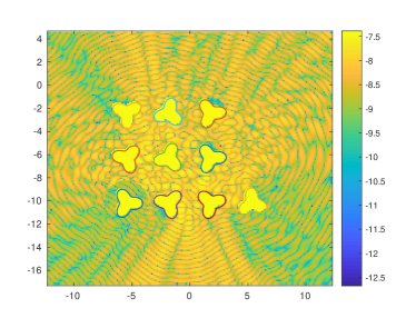
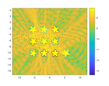
Figure 2 shows the error of the computed elastic field compared with the analytic solution when ω=4π𝜔4𝜋\omega=4\pi by the scattering matrix based method. The near field is evaluated by the QBX [16], i.e., the field near the boundary of each particle is evaluated by the use of local expansions formed by the FMM. Overall the error is less than 1E-7. We also show the 
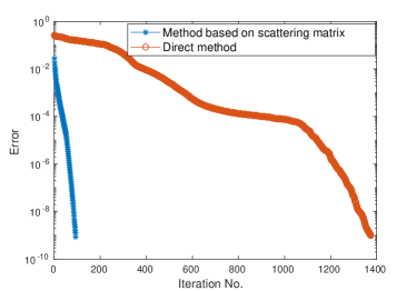
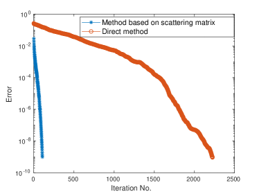
comparison of convergence rate between the direct method and our method in Figure 2(c), 2(d). Obviously, one can see a much faster convergence for the scattering matrix based method.

Refer to caption
Refer to caption

(a)                                                              (b)
Refer to caption Refer to caption
(c)                                                              (d)

Figure 2. Elastic scattering of 10 particles at $\omega=4\pi$. (a) The logarithmic error of the computed field when $a=1$, $b=1/3$, $c=3$. (b) The logarithmic error of the computed field when $a=1$, $b=1/3$, $c=5$. (c) Comparison of the GMRES convergence rate when $a=1$, $b=1/3$, $c=3$. (d) Comparison of the GMRES convergence rate when $a=1$, $b=1/3$, $c=5$. More details are given in the text of Example 1.
$a=1$, $b=\frac{1}{3}$, $c=3$ $a=1$, $b=\frac{1}{3}$, $c=5$
$\omega$ $N_{pts}$ $N_{tot}$ $N_{iter}$ $T_{solve}$ $E_{err}$ $N_{iter}$ $T_{solve}$ $E_{err}$
50 1000 930 7.96E1 5.79E-4 943 7.84E1 2.12E-2
$\pi$ 100 2000 1071 1.79E2 1.36E-6 1613 2.75E2 2.17E-7
200 4000 2243 7.23E2 4.47E-10 2814 1.01E3 2.56E-9
50 1000 930 7.92E1 5.79E-4 933 8.02E1 2.75E-3
$2\pi$ 100 2000 1410 2.43E2 8.08E-7 1588 2.78E2 2.63E-5
200 4000 2243 7.26E2 4.47E-10 2327 8.15E2 7.94E-9
50 1000 847 7.42E1 2.12E-3 993 8.92E1 1.72E-2
$4\pi$ 100 2000 939 1.61E2 1.04E-6 1670 3.01E2 5.27E-5
200 4000 1374 4.29E2 8.11E-10 2225 8.22E2 2.47E-8
Table 1. Example 1: Results for the elastic scattering of 10 particles based on the direct method with FMM acceleration.
$a=1$, $b=\frac{1}{3}$, $c=3$ $a=1$, $b=\frac{1}{3}$, $c=5$
$\omega$ $N_{term}$ $N_{tot}$ $N_{iter}$ $T_{solve}$ $E_{err}$ $N_{iter}$ $T_{solve}$ $E_{err}$
10 420 63 4.01E-2 8.35E-6 67 4.02E-2 6.59E-6
$\pi$ 20 820 62 8.81E-2 4.71E-9 67 9.61E-2 6.17E-9
40 1620 61 2.39E-1 5.75E-9 67 2.72E-1 6.84E-10
10 420 74 4.81E-2 3.39E-5 88 6.01E-2 8.41E-5
$2\pi$ 20 820 73 1.07E-1 6.49E-9 87 1.24E-1 5.32E-9
40 1620 73 2.91E-1 2.09E-9 87 3.61E-1 2.31E-9
10 420 94 6.39E-2 1.84E-2 104 7.21E-2 1.70E-2
$4\pi$ 20 820 94 1.41E-1 7.85E-7 108 1.64E-1 1.72E-7
40 1620 93 3.84E-1 3.42E-9 107 4.47E-1 1.12E-8
Table 2. Example 1: Results for the elastic scattering of 10 particles by using the scattering matrix based method with FMM acceleration.

6.2. Example 2: point source incidence

In this example, we test our algorithm on a large number of rigid particles with point source incidence. The point source is given by the form of equation (6.1) with $x_{0}=(5,5)$ and all the particles are randomly located in the lower half plane. To ensure that the particles are well separated but confined in a fixed region, we use a bin sorting algorithm to construct the random distribution, i.e., we begin with particles located on a regular grid and then perturb their positions randomly several times. The details can be found in [19].

We construct the scattering matrix by solving the integral equation (4.1) on a single particle with 200 discretization points. The number of terms in the multipole expansion is chosen to be $N_{term}=20$. To verify the accuracy of the computed solution, we compare it with the solution obtained by choosing $N_{term}=40$. Numerical results for various angular frequencies are shown in Table 3 and Figure 3. From Table 3, we can see that the number of iterations grows roughly linearly with respect to the angular frequency $\omega$ for a fixed number of particles. If $\omega$ is fixed, the number of iterations increases sublinearly with respect to the number of particles. Another observation is that the field is mainly affected by the size of a particle, not by the detailed geometry, since the number of iterations is almost constant when we change the value of $c$, which controls how many ‘leaves’ that a particle has. The total field plotted in Figure 3 for scattering of $1000$ particles also confirms this observation. We have to note, however, that this conclusion may only hold when the size of each particle is in subwavelength regime for a given incident field.

Refer to caption
Refer to caption

(a)                                                              (b)
Refer to caption Refer to caption
(c)                                                              (d)

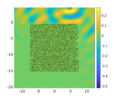
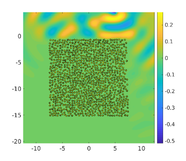
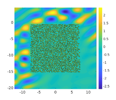
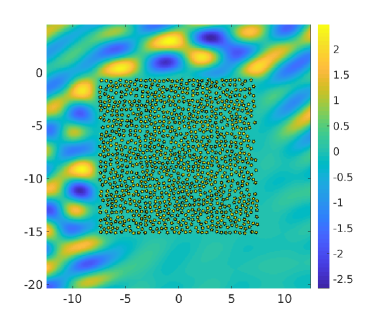
Figure 3. The elastic scattering of 1000 particles by point source illumination in Example 2. Here we show the real part of the first component of the total elastic field. (a) Field for $a=\frac{1}{8}$, $b=\frac{1}{24}$, $c=3$, $\omega=\pi$. (b) Field for $a=\frac{1}{8}$, $b=\frac{1}{24}$, $c=5$, $\omega=\pi$. (c) Field for $a=\frac{1}{8}$, $b=\frac{1}{24}$, $c=3$, $\omega=4\pi$. (d) Field for $a=\frac{1}{8}$, $b=\frac{1}{24}$, $c=5$, $\omega=4\pi$.
$a=\frac{1}{8}$, $b=\frac{1}{24}$, $c=3$ $a=\frac{1}{8}$, $b=\frac{1}{24}$, $c=5$
$\omega$ $N_{particle}$ $N_{tot}$ $N_{iter}$ $T_{solve}$ $E_{err}$ $N_{iter}$ $T_{solve}$ $E_{err}$
100 8400 57 3.51E0 1.38E-9 59 3.41E0 1.62E-10
$\pi$ 500 42000 130 5.28E1 9.39E-10 131 5.21E1 2.21E-9
1000 82000 210 1.34E2 9.62E-10 212 1.36E2 2.81E-9
100 8400 96 6.09E0 1.64E-9 97 5.86E0 4.24E-9
$2\pi$ 500 42000 249 1.05E2 4.10E-9 251 1.06E2 3.71E-9
1000 84000 347 2.48E2 1.03E-9 353 2.53E2 3.34E-9
100 8400 271 1.79E1 4.22E-9 255 1.65E1 6.31E-9
$4\pi$ 500 42000 614 3.09E2 1.63E-9 667 3.43E2 2.54E-9
1000 84000 1197 1.31E3 7.69E-10 1211 1.34E3 7.42E-9
Table 3. Example 2: Results for the elastic scattering of multiple particles by using the scattering matrix based method with FMM acceleration.

6.3. Example 3: plane incidence wave

For the third example, we evaluate the elastic scattered field of a large number of particles by plane wave incidence, which is given by

$\displaystyle{\bf u}^{\rm inc}=de^{{\rm i}k_{p}x\cdot d}+d^{\perp}e^{{\rm i}k_{s}x\cdot d},$

where $d$ is the propagation direction. In our test, we choose $d=(\cos(-\frac{\pi}{3}),\sin(-\frac{\pi}{3}))$. The location of particles are randomly distributed in a fixed region which is the same as that in Example 2. The transformation of plane wave into the local expansion (5.1) is given by the Jacobi–Anger identity[25]. Numerical results for the plane wave incidence are given in Figure 4 and Table 4. Comparing the results between Tables 2 and 4, we find that the number of iterations for the plane wave incidence is similar to the one with the point source incidence. In particular, the results for both the point source incidence and the plane wave incidence show that the number of iterations for GMRES does depend on the size of particles but is almost independent of the shape of particles. This fact is further illustrated by Figure 4, since the fields for two different kind particles looks almost identical. Again, the conclusion may only hold if we restrict in the subwavelength regime. Another observation from Figure 4 is that when the average distance among particles is small, the scattered field acts as if there exists a large obstacle. How to quantify such an equivalence will be explored in our future investigation.

Refer to caption
Refer to caption

(a)                                                              (b)
Refer to caption Refer to caption
(c)                                                              (d)

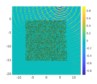
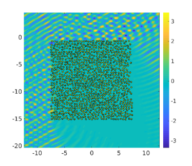
Figure 4. The elastic scattering of 1000 particles by the plane wave incidence in Example 3. Here we show the real part of the first component of the total elastic field. (a) Field for $a=\frac{1}{8}$, $b=\frac{1}{24}$, $c=3$, $\omega=\pi$. (b) Field for $a=\frac{1}{8}$, $b=\frac{1}{24}$, $c=5$, $\omega=\pi$. (c) Field for $a=\frac{1}{8}$, $b=\frac{1}{24}$, $c=3$, $\omega=4\pi$. (d) Field for $a=\frac{1}{8}$, $b=\frac{1}{24}$, $c=5$, $\omega=4\pi$.
$a=\frac{1}{8}$, $b=\frac{1}{24}$, $c=3$ $a=\frac{1}{8}$, $b=\frac{1}{24}$, $c=5$
$\omega$ $N_{particle}$ $N_{tot}$ $N_{iter}$ $T_{solve}$ $E_{err}$ $N_{iter}$ $T_{solve}$ $E_{err}$
100 8400 64 4.49E0 1.75E-9 66 3.68E0 8.66E-10
$\pi$ 500 42000 140 5.62E1 2.21E-9 142 5.79E1 3.33E-9
1000 82000 221 1.47E2 2.44E-9 224 1.55E2 4.97E-9
100 8400 101 7.36E0 7.76E-10 103 6.34E0 3.85E-9
$2\pi$ 500 42000 271 1.17E2 1.32E-9 273 1.19E2 7.06E-9
1000 84000 384 2.93E2 2.09E-9 391 2.93E2 1.01E-8
100 8400 287 1.91E1 1.05E-8 270 1.89E1 3.48E-8
$4\pi$ 500 42000 693 3.70E2 6.21E-9 727 4.10E2 1.01E-8
1000 84000 1459 1.95E3 1.03E-9 1433 1.78E3 2.62E-8
Table 4. Example 3: Results for the elastic scattering of multiple particles by using the scattering matrix based method with the FMM acceleration.

7. Conclusion

In this paper, we have studied the elastic scattering problem with multiple rigid particles by using the Helmholtz decomposition. Three different integral formulations are presented for the coupled Helmholtz system. Their well-posedness are studied by using appropriate regularizers. A fast numerical method is proposed for the elastic scattering of multiple arbitrarily shaped obstacles. The idea is to construct the scattering matrix based on the proposed integral formulation for a single particle, and then extend the multiple scattering theory from acoustic waves to elastic waves. In the end, the resulted linear equation is solved by the GMRES with the FMM acceleration. Numerical results show that our algorithm is much faster than the one that directly discretizes particles by points. In particular, we show that the method can achieve high order accuracy even for the scattering of up to 1000 elastic particles. The method can be extended to the three-dimensional elastic wave scattering problem where the Helmholtz decomposition involves a scalar potential function and a vector potential function. The progress will be reported elsewhere in the future.

References

  • [1] J. F. Ahner, G. C. Hsiao, On the two-dimensional exterior boundary-value problems of elasticity, SIAM J. Appl. Math., 31 (1976), 677–685.
  • [2] B. K. Alpert, Hybrid Gauss-trapezoidal quadrature rules, SIAM J. Sci. Comput., 20 (1999), 1551–1584.
  • [3] H. Ammari, E. Bretin, J. Garnier, H. Kang, H. Lee, and A. Wahab, Mathematical Methods in Elasticity Imaging, Princeton University Press, New Jersey, 2015.
  • [4] G. Bao, K. Huang, P. Li, and H. Zhao, A direct imaging method for inverse scattering using the generalized Foldy–Lax formulation, Contemp. Math., 615 (2014), 49–70.
  • [5] G. Bao, L. Xu, and T. Yin, An accurate boundary element method for the exterior elastic scattering problem in two dimensions, J. Comput. Phys., 348 (2017), 343–363.
  • [6] F. Bu, J. Lin, and F. Reitich, A fast and high-order method for the three-dimensional elastic wave scattering problem, J. Comput. Phys., 258 (2014), 856–870.
  • [7] D. Colton and R. Kress, Integral Equation Method in Scattering Theory, Wiley-Interscience, New York, 1983.
  • [8] Z. Gimbutas and L. Greengard, Fast multi-particle scattering: A hybrid solver for the Maxwell equations in microstructured materials, J. Comput. Phys., 232 (2012), 22–32.
  • [9] D. Givoli and J. B. Keller, Non-reflecting boundary conditions for elastic waves, Wave Motion, 12 (1990), 261–279.
  • [10] L. Greengard and V. Rokhlin, A fast algorithm for particle simulations, J. Comput. Phys., 73 (1987), 325–348.
  • [11] M. J. Grote and C. Kirsch, Dirichlet-to-Neumann boundary conditions for multiple scattering problems, J. Comput. Phys., 201 (2004), 630–650.
  • [12] G. Hu, A. Kirsch, and M. Sini, Some inverse problems arising from elastic scattering by rigid obstacles, Inverse Problems, 29 (2013), 015009
  • [13] K. Huang and P. Li, A two-scale multiple scattering problem, Multiscale Model. Simul., 8 (2010), 1511–1534.
  • [14] K. Huang, P. Li, and H. Zhao, An efficient algorithm for the generalized Foldy–Lax formulation, J. Comput. Phys., 234 (2013), 376–398.
  • [15] X. Jiang and W. Zheng, Adaptive perfectly matched layer method for multiple scattering problems, Comput. Methods Appl. Mech. Engrg., 201 (2012), 42–52.
  • [16] A. Klöckner, A. Barnett, L. Greengard, and M. O’Neil, Quadrature by expansion: A new method for the evaluation of layer potentials, J. Comput. Phys., 252 (2013), 332–349.
  • [17] R. Kress, Linear Integral Equations, Springer, New York, 1999.
  • [18] J. Lai, M. Kobayashi, and A. Barnett, A fast and robust solver for the scattering from a layered periodic structure containing multi-particle inclusions, J. Comput. Phys., 298 (2015), 194–208.
  • [19] J. Lai, M. Kobayashi, and L. Greengard, A fast solver for multi-particle scattering in a layered medium, Opt. Express, 22 (2014), 20481–20499.
  • [20] L. D. Landau and E. M. Lifshitz, Theory of Elasticity, Oxford: Pergamon 1986.
  • [21] P. Li, Y. Wang, Z. Wang, and Y. Zhao, Inverse obstacle scattering for elastic waves, Inverse Problems, 32 (2016), 115018.
  • [22] F. Le Louër, On the Fréchet derivative in elastic obstacle scattering, SIAM J. Appl. Math., 72 (2012), 1493–1507.
  • [23] P. Martin, Multiple Scattering: Interaction of Time-Harmonic Wave with $N$ Obstacles, Encyclopedia Math. Appl. 107, Cambridge University Press, Cambridge, 2006.
  • [24] J.-C. Nédélec, Acoustic and Electromagnetic Equations: Integral Representation for Harmonic Problems, Springer, New York, 2000.
  • [25] F. W. J. Olver, D. W. Lozier, R. F. Boisvert, and C. W. Clark, NIST Handbook of Mathematical Functions, Cambridge University Press, New York, 2010.
  • [26] Y. H. Pao and V. Varatharajulu, Huygens’ principle, radiation conditions, and integral formulas for the scattering of elastic waves, J. Acoust. Soc. Amer., 59 (1976), 1361–1371.
  • [27] B. Peterson and S. Ström, $T$ matrix for electromagnetic scattering from an arbitrary number of scatterers and representations of E(3), Phys. Rev. D, 8 (1973), 3661–3678.
  • [28] V. Rokhlin, Rapid solution of integral equations of scattering theory in two dimensions, J. Comput. Phys., 86 (1990), 414–439.
  • [29] A. Sommerfeld, Partial Differential Equations in Physics, Academic Press, New York, 1949.
  • [30] M. S. Tong and W. C. Chew, Nyström method for elastic wave scattering by three-dimensional obstacles, J. Comput. Phys., 226 (2007), 1845–1858.
  • [31] M. S. Tong and W. C. Chew, Multilevel fast multipole algorithm for elastic wave scattering by large three-dimensional objects, J. Comput. Phys., 228 (2009), 921–932.
  • [32] T. Yin, G. C. Hsiao, and L. Xu, Boundary integral equation methods for the two-dimensional fluid-solid interaction problem, 55 (2017), SIAM J. Numer. Anal., 2361–2393.
  • [33] J. Yue, M. Li, P. Li, and X. Yuan, Numerical solution of an inverse obstacle scattering problem for elastic waves via the Helmholtz decomposition, Commun. Comput. Phys., to appear.