Compton-thick AGN in the NuSTAR era IV: A deep NuSTAR and XMM-Newton view of the candidate Compton thick AGN in ESO 116-G018

Abstract

We present the 2–78 keV spectral analysis of the deep NuSTAR and XMM-Newton observation of a nearby Seyfert 2 galaxy, ESO 116-G018, which is selected as a candidate Compton-thick (CT-) active galactic nucleus (AGN) based on a previous Chandra-Swift-BAT study. Through our analysis, the source is for the first time confirmed to be a CT-AGN at a $>$3 $\sigma$ confidence level, with the “line-of-sight” column density N_H,Z = [2.46–2.76] $\times$ $10^{24}$ cm^-2. The “global average” column density of the obscuring torus is N_H,S = [0.46–0.62] $\times$ $10^{24}$ cm^-2, which suggests a clumpy, rather than uniform, distribution of the obscuring material surrounding the accreting supermassive black hole. The excellent-quality data given by the combined NuSTAR and XMM-Newton observations enable us to produce a strong constraint on the covering factor of the torus of ESO 116-G018, which is found to be $f_{c}$ = [0.13-0.15]. We also estimate the bolometric luminosity from the broad-band X-ray spectrum, being L_bol = [2.57–3.41] $\times$ 10⁴⁴ erg s^-1.

1. Introduction

The intrinsic emission from an accreting supermassive black hole (SMBH), i.e., the center of active galactic nuclei (AGNs), is commonly believed to be, at least partly, obscured by the circumnuclear matter. Especially, AGN are classified as Compton-thick (CT-) AGNs when the column density of the obscured matter is N_H $\geq$ $\sigma_{T}^{-1}$ $\sim$10²⁴ cm^-2, where $\sigma_{T}$ is the Thomson cross section. Knowing the distribution of the absorbing column density is not only important to understand the physics of the accreting SMBHs, but is also essential to properly model the cosmic X-ray background (CXB), i.e., the diffused X-ray emission observed between 0.5 keV and 300 keV, which is believed to be mainly produced by both obscured and unobscured AGNs. While most of the CXB emission below 10 keV has been resolved thanks to Chandra and XMM-Newton (see, e.g., Worsley et al., 2005; Hickox & Markevitch, 2006), only $\sim$35% of the CXB emission at its peak ($\sim$30 keV, Ajello et al., 2008) has been resolved, mostly by different NuSTAR surveys (Aird et al., 2015; Harrison et al., 2016). In this energy range, CT-AGNs are expected to be numerous (up to 50% of the overall population of Seyfert 2 galaxies, see, e.g., Risaliti et al., 1999). Different CXB synthesis models predict that the fraction of CT-AGN should be $\sim$20%–30% (Alexander et al., 2003; Gandhi & Fabian, 2003; Gilli et al., 2007; Treister et al., 2009; Ueda et al., 2014). However, as of today CT-AGNs have never been detected in large numbers, e.g., their observed fraction in the local universe is $\sim$5–10% (see, e.g. Burlon et al., 2011; Ricci et al., 2015) in the X-rays and is $\sim$12% when performing a multi-wavelength search (Goulding et al., 2011).

Due to the heavy obscuration, CT-AGNs are difficult to detect below $\sim$10 keV in the local universe (see, e.g., Gilli et al., 2007; Koss et al., 2016), since the overall X-ray emission in these objects is suppressed below 10 keV and dominated by the Compton hump at $\sim$20–40 keV. CT-AGNs at redshift $z>$1 can instead be well studied using one of the several facilities sampling the $\sim$0.3–10 keV energy range, such as Swift-XRT, Chandra, XMM-Newton and Suzaku (see, e.g., Georgantopoulos et al., 2013; Buchner et al., 2015; Lanzuisi et al., 2015): the Compton hump of high-$z$ sources is redshifted in the energy range covered by these instruments. However, for sources in the local universe ($z$ $<$0.1), the proper characterization of heavily obscured AGN requires an X-ray telescope sensitive above 10 keV. Thanks to the launch of Nuclear Spectroscopic Telescope Array (hereafter, NuSTAR, Harrison et al., 2013), which provides a two orders of magnitude better sensitivity than previous telescopes (e.g., INTEGRAL and Swift-BAT; Winkler et al., 2003; Barthelmy et al., 2005) at $\sim$10–50 keV, one can study the physical and geometrical properties of heavily obscured AGN with unprecedented accuracy (see, e.g. Baloković et al., 2014; Puccetti et al., 2014; Annuar et al., 2015; Marchesi et al., 2017b, 2018; Ursini et al., 2018). To properly constrain both the torus column density and the AGN photon index in heavily obscured sources, however, one needs to combine the excellent NuSTAR effective area at energies $>$10 keV with a soft X-ray instrument, which covers the 0.5–10 keV energy range. Among these, XMM-Newton is the best one in terms of both effective area in the 0.3–10 keV energy range and spectral energy resolution (150 eV, $\sim$2.5 better than NuSTAR, which has $\Delta$E = 400 eV) at the energy of the Fe K$\alpha$ line (the signature of obscured AGN at E=6.4 keV).

The obscuration observed in AGNs across the electromagnetic spectrum, from X-ray to infrared, is usually explained with a pc-scale, torus-like structure of dust and gas (see, e.g., Almeida & Ricci, 2017). Consequently, several tori models, based on Monte Carlo simulations, have been developed to characterize the X-ray spectra of CT-AGNs in the past two decades (Matt & Fabian, 1994; Ikeda et al., 2009; Murphy & Yaqoob, 2009; Brightman & Nandra, 2011; Liu & Li, 2014; Furui et al., 2016; Baloković et al., 2018). All these models assume a continuous distribution of the obscuring material, but with a different assumption on the geometry of the torus. In particular, in the models proposed by Ikeda et al. (2009), Brightman & Nandra (2011) and Baloković et al. (2018), the half opening angle of the torus, i.e., the torus covering factor, is a free parameter, thus allowing to put constraints on the toroidal geometry. Given the intrinsic complexity of these models, and the multiple free parameters involved, applying them in full capability requires high-quality X-ray spectra, with excellent statistics on a wide energy range, i.e., between 1 and 100 keV: at the present day, similar requirements can be satisfied only by a joint NuSTAR and XMM-Newton observation. The AGN emission can also be observed at infrared wavelengths, where part of the intrinsic accretion disk optical-UV emission is absorbed by the dust in the “torus-like” structure and then re-emitted in the infrared. Thus, the fraction of the luminosity of the torus with respect to the AGN bolometric luminosity ($L_{\rm tor}$/$L_{\rm AGN}$) can be used as a proxy of the torus covering factor (see; e.g. Stalevski et al., 2016). Indeed, in addition to the previously mentioned X-ray models, theory and models on the nature of the obscuration from an infrared perspective have also been developed (Krolik & Begelman, 1988; Jaffe et al., 2004; Tristram et al., 2007; Nenkova et al., 2008; Hönig & Kishimoto, 2010; Stalevski et al., 2012).

In this work, we present the results of a deep, 50 ks combined NuSTAR and XMM-Newton observation of ESO 116-G018, a nearby Seyfert 2 galaxy and a candidate CT-AGN. The paper is organized as follows: in Section 2 , we report the NuSTAR and XMM-Newton data reduction and spectral extraction process; in Section 3, we describe the different models which are used to fit the broadband X-ray spectra, and the results of the spectral analysis using above models; in Section 4, we compare our results with those already existent in the literature, and discuss the constraints on the physical properties of ESO 116-G018, e.g., the equivalent width of the iron K$\alpha$ line and the intrinsic luminosity, and the geometry, i.e., covering factor, of the obscuring “torus-like” structure. All reported uncertainties on spectral parameters are at 90% confidence level, if not otherwise stated. Standard cosmological constants are adopted as follows: $<H_{0}>$ = 70 km s^-1 Mpc^-1, $<q_{0}>$ = 0.0 and $<\Lambda>$ = 0.73.

2. Observation and Data Analysis

ESO 116-G018 ($z$ $\sim$0.0185, $d$ $\sim$80 Mpc, de Grijp et al., 1992) is a Seyfert 2 galaxy which is detected in the 100-month BAT catalog (Segreto et al. 2019 in prep.), a catalog of $\sim$1000 AGNs detected by Swift-BAT in the 15–150 keV band.

ESO 116-G018 was first selected as a candidate CT-AGN by Marchesi et al. (2017a) using the selection technique described in the paper and then was targeted with a 10 ks follow-up observation with Chandra. The joint Chandra–Swift-BAT spectral fit allowed us to obtain a first measurement of the source “line-of-sight” column density, which is N_H,Z = 0.95${}_{-0.40}^{+0.46}$ $\times$ $10^{24}$ cm^-2. The low-quality of the Chandra spectrum ($\sim$50 net counts in the 0.5–7 keV band) prevented us to properly characterize ESO 116-G018, or even confirm or reject its Compton-thick origin at a $>$3 $\sigma$ confidence level. Therefore, to further investigate this new candidate CT-AGN, as well as another one, NGC 1358, which we analyzed in a companion paper (Zhao et al. 2018 submitted), we proposed for a simultaneous NuSTAR (45 ks) and XMM-Newton (58 ks) follow-up observation, which was accepted in NuSTAR Cycle 3 (proposal ID 3258, PI: Marchesi). We report a summary of the observations in Table 1.

Table 1Summary of NuSTAR and XMM-Newton observations.

Instrument	Sequence	Start Time	End Time	Exposure Time	Count Rate
	ObsID	(UTC)	(UTC)	(ks)	$10^{-2}$counts s-1
NuSTAR	60301027002	2017-11-01T18:56:09	2017-11-02T20:46:09	45	1.24$\pm$0.06 1.31$\pm$0.06
XMM-Newton	0795680201	2017-11-01T19:19:57	2017-11-02T11:32:32	58	0.33$\pm$0.02 0.44$\pm$0.03 1.58$\pm$0.06

The reported NuSTAR count rates are those of the FPMA and FPMB modules between 3–78 keV, respectively. The reported XMM-Newton count rates are those the MOS1, MOS2 and pn modules between 2–10 keV, respectively.

2.1. NuSTAR Observation

ESO 116-G018 was observed by NuSTAR on 2017 November 1–2 (ObsID 60301027002). The observation took place in a 95.5 ks time-span and was divided into 15 ($\sim$3 ks) intervals. The gaps in the observation correspond to the periods of time in which the target was occulted by the Earth. The NuSTAR data is derived from both focal plane modules, FPMA and FPMB. The raw files are calibrated, cleaned and screened using the NuSTAR nupipeline script version 0.4.5. The NuSTAR calibration database (CALDB) used in this work is version 20171002. The ARF, RMF and light-curve files are obtained using the nuproducts script. For both modules, the source spectrum is extracted from a 30^′′ circular region, corresponding to $\approx$50% of the encircled energy fraction (EEF) at 10 keV, centered on the source optical position. We then extract a background spectrum for each module, choosing a 30^′′ circular region located nearby the outer edges of the field of view, to avoid contamination from the source and no flares are found in the background light curves. The NuSTAR spectra are grouped with a minimum of 15 counts per bin using the HEAsoft task grppha.

2.2. XMM-Newton Observation

The XMM-Newton observation was taken quasi-simultaneously to the NuSTAR one with the EPIC CCD cameras (pn; Strüder et al., 2001) and two MOS cameras (Turner et al., 2001): the XMM-Newton observation started at the same time, but ended $\sim$9 hours before the NuSTAR one. We reduced the XMM-Newton data using the Science Analysis System (SAS; Jansen et al., 2001) version 16.1.0. The source spectra are extracted from a 15^′′, corresponding to $\approx$70% of the encircled energy fraction (EEF) at 1.5 keV, circular region, while the background spectra are obtained from an 80^′′ circle located nearby the source. We visually inspected the XMM-Newton image to avoid contamination to the background from sources nearby ESO 116-G018.

2.3. Variability

When visually inspecting the light curves of both NuSTAR (3–78 keV) and XMM-Newton (2–10 keV) of ESO 116-G018, we find no obvious evidence of variability during the observations. The background subtracted light curves of NuSTAR module FPMA and XMM-Newton EPIC MOS1 are presented in Figure 1. We further analyze the two light curves by fitting them with a constant, $r$, which corresponds to the average count rate: we use the $\chi^{2}$ test to check for any statistical evidence of variability. The best-fit average count rate is $r_{\rm FPMA}$ = 1.3$\pm{0.3}$ $\times$ 10^-2 cts s^-1 for the NuSTAR module FPMA; the $\chi^{2}$ for the fit is $\chi^{2}_{\rm FPMA}$ = 4.4 with 10 degrees of freedom, while the light curve would be different from a constant at a the $>$99% confidence level if $\chi^{2}$ $>$23.2 for 10 degrees of freedom. The best-fit average count rate of XMM-Newton EPIC MOS1 is $r_{\rm MOS1}$ = 3.2$\pm{0.7}$ $\times$ 10^-3 cts s^-1; the $\chi^{2}$ for the fit is $\chi^{2}_{\rm MOS1}$ = 4.9, while the light curve would be different from a constant at a the $>$99% confidence level if $\chi^{2}$ $>$16.8 for 6 degrees of freedom.

Based on the fit statistics given above, there is no significant variability in both the NuSTAR and the XMM-Newton light curve of ESO 116-G018.

Figure 1.— Background subtracted light curves of NuSTAR module FPMA (left panel) XMM-Newton module MOS1 (right panel). The bin time is equal to 9 ks for both light curves. The average count rates are $r_{\rm FPMA}$ = 1.3$\pm{0.3}$ $\times$ 10^-2 cts s^-1 for FPMA and r_MOS1 = 3.2$\pm{0.7}$ $\times$ 10^-3 cts s^-1 for MOS1, respectively.

3. Spectral Modeling Results

We performed the spectral fit of ESO 116-G018 using XSPEC v12.9.1 (Arnaud, 1996) and the $\chi^{2}$ statistic. The photoelectric cross section for all absorption components used are those from Verner et al. (1996). The element abundance is from Anders & Grevesse (1989) and metal abundance is fixed to Solar. The Galactic absorption column density is N_H,Gal = $3.1\times 10^{20}$ cm^-2 (Kalberla et al., 2005). The source redshift is fixed at $z$ = 0.0185.

Following a standard approach in analyzing heavily obscured AGN, we begin our spectral modeling using the phenomenological model. We report in Table 2 the results of the joint NuSTAR–XMM-Newton spectral fitted using the different models which will be discussed in the following sections.

3.1. Phenomenological Model

We first fit the spectra with a phenomenological model composed of an absorbed power law with photon index $\Gamma$. The absorption caused by the obscuring gas and dust surrounding the accreting SMBH is modeled by zphabs, while the Galactic absorption is modeled by phabs. We also add to the model a Gaussian (zgauss) to characterize the prominent Fe K$\alpha$ line typically observed in heavily obscured AGNs. We fix the center of the Gaussian at 6.4 keV and fix the line width $\sigma$ to 50 eV, assuming the line to be narrow, to minimize the number of free parameters: nonetheless, no significant improvement is found when leaving the line width free to vary. Below $\sim$5 keV, the spectrum is dominated by the fraction (usually less than 5–10%, see, e.g., Marchesi et al., 2018) of emission from the intrinsic X-ray continuum, which is not intercepted by the torus on the “line-of-sight”, and/or the intrinsic emission is deflected, rather than absorbed by the obscuring material into the “line-of-sight”. This scattered component is modeled by an unabsorbed power law having photon index $\Gamma_{2}$ = $\Gamma$: the fractional intensity with respect to the intrinsic emission, $f_{s}$, is modeled by a constant ($constant_{2}$).

Finally, the cross-calibration between NuSTAR and XMM-Newton is modeled by another constant ($constant_{1}$), noted as $C_{NuS/XMM}$. We also assume that there is no flux offset between different modules of the same instrument. The phenomenological model (Model A), in XSPEC nomenclature, is thus:

$$ModelA= constant_{1}*phabs*(zphabs*zpowerlw$$ (1)

$$+zgauss+constant_{2}*zpowerlw)$$

The best-fit results of model A is reported in Table 2 and Fig. 2 shows the best-fit of the spectra of ESO 116-G018 fitted with model A. The best-fit intrinsic photon index is $\Gamma$ = 0.99${}_{-0.12}^{+0.13}$ and the column density of the obscuring material along our “line-of-sight” is N_H = 0.62${}_{-0.12}^{+0.12}$ $10^{24}$ cm^-2. Although the statistics ($\chi^{2}_{\nu}$ = $\chi^{2}$/degrees of freedom, d.o.f. hereafter, = 166/162 = 1.02) of the phenomenological model is acceptable, the best-fit photon index, $\Gamma$ = 0.99${}_{-0.12}^{+0.13}$, is not physically plausible (typical AGNs have photon indices within the range $\Gamma$ = 1.4–2.6; see, e.g., Murphy & Yaqoob, 2009). This is not an unexpected result, since the complexity of the spectral shape of a heavily obscured AGN cannot be properly treated by a standard absorption component alone such as zphabs: such a model cannot, for example, properly model the shape of the reprocessed component known as “Compton hump” observed at energies $E$ $\sim$10–40 keV.

In the next section, we, therefore, fit the data with physically motivated models, i.e.,pexrav (Magdziarz & Zdziarski, 1995), MYTorus (Murphy & Yaqoob, 2009) and borus02 (Baloković et al., 2018), which are suitable to characterize heavily obscured AGNs with high-quality X-ray spectra.

3.2. Physical Models

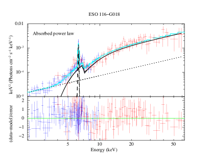
Figure 2.— Unfolded XMM-Newton and NuSTAR spectrum of ESO 116-G018 fitted with model A (top). The XMM-Newton data are plotted in blue, while the NuSTAR data are plotted in red. The best-fit models prediction is plotted as a cyan solid line. The single components of the model are plotted in black with different line styles, i.e., the absorbed intrinsic continuum as a solid line, the Fe K$\alpha$ line as a dashed line and the scattered component as a dotted line.

3.2.1 Absorbed power-law with reflection component

pexrav has historically been used to model heavily obscured AGN spectra where the observed emission is dominated by the photons reprocessed and upscattered by the obscuring material. pexrav models a power law spectrum with an exponential cut off reflected from a slab of neutral material. We first test the pexrav model utilized as a pure reflector by setting the reflection scaling factor to be R = -1, assuming the “line-of-sight” is heavily obscured (e.g., when N_H $\geq$10²⁵ cm^-2) such that the observed spectrum is entirely contributed by the reflection from the back-side of the obscuring matter. The photon index is $\Gamma$ = 1.57${}_{-0.09}^{+0.09}$ with the reduced $\chi^{2}$ to be $\chi^{2}_{\nu}$ = 167/163 = 1.02. Although the pure reflection component fits the reprocessed emission at 10–40 keV well, it fails to describe the soft X-ray part at $E$ $<$10 keV. Therefore, we add an absorbed power law to model the “line-of-sight” continuum following the method adopted in Ricci et al. (2011).

In the XSPEC nomenclature, our pexrav model is written as follows:

$$ModelB= constant_{1}*phabs*(zphabs*zpowerlw+$$ (2)

$$pexrav+zgauss+constant_{2}*zpowerlw)$$

where all the components other than pexrav are those already described in the previous section. While in pexrav, the inclination angle $i$, i.e., the angle between the axis of the AGN (normal to the disk) and the observer line of sight, is fixed to $i$ = 60^∘ (cos $i$ = 0.5). We do not find any significant variation in the spectral fit results when adopting other two inclination angle values, i.e., $i$ = 87^∘ and 18^∘ (cos $i$ = 0.05 and 0.95). The cut-off energy is fixed at $E_{cut}$ = 500 keV to be consistent with the MYTorus model, which will be discussed in detail in the following section: no significant improvement is found when we leave the cut-off energy free to vary. Finally, the reflection scaling factor $R$ is set to be less than 0 (i.e., the model describes only the reprocessed component) and is free to vary.

We show in Fig. 3 the best-fit of the joint XMM-Newton–NuSTAR spectra obtained using Model B. The best-fit photon index is $\Gamma$ = 1.54${}_{-0.19}^{+0.18}$ and the “line-of-sight” column density is N_H,Z = 0.88${}_{-0.26}^{+0.32}$ $\times$ $10^{24}$ cm^-2. It is worth noting that, although the pexrav result, with the reduced $\chi^{2}$ being $\chi^{2}_{\nu}$ = $\chi^{2}$/d.o.f. = 145/161 = 0.90, is improved with respect to the one of Model A, different components of the spectrum, e.g., the iron line (modeled by a Gaussian), are not treated in a self-consistent way.

In summary, according to both model A and model B, ESO 116-G018 is heavily obscured but not Compton-thick. However, in model A, the photon index $\Gamma$ is significantly harder than the one of a typical obscured AGN; furthermore, the fraction of scattered emission is slightly larger than the typical 1–10% value in both models, being $f_{s}$ $\sim$11%. Model B (pexrav), in spite of a significant improvement in statistics and a reasonable photon index, fails to treat the reprocessed components, i.e., the reflection component and the fluorescent lines, self-consistently. Therefore, in order to better unveil the physics of the obscuring matter surrounding the accreting SMBH of ESO 116-G018, more self-consistent and realistic models are needed.

Table 2Summary of Best-Fits of XMM-Newton and NuSTAR Data using Different Models.

Model	phenom	pexrav	MYTorus	MYTorus	MYTorus	borus02
			(coupled)	(decoupled face on)	(decoupled edge on)
$\chi^{2}$/d.o.f.	166/162	145/161	140/161	150/161	144/161	140/160
$C_{Ins}$	0.99${}_{-0.12}^{+0.13}$	1.03${}_{-0.12}^{+0.13}$	1.06${}_{-0.08}^{+0.08}$	1.01${}_{-0.13}^{+0.14}$	1.07${}_{-0.14}^{+0.15}$	1.07${}_{-0.08}^{+0.08}$
$\Gamma$	0.99${}_{-0.18}^{+0.19}$	1.54${}_{-0.19}^{+0.18}$	1.79${}_{-0.12}^{+0.11}$	1.51${}_{-0.11}^{+0.37}$	1.74${}_{-0.34}^{+0.40}$	1.80${}_{-0.06}^{+0.06}$
norm 10-3	0.07${}_{-0.03}^{+0.06}$	0.17${}_{-0.09}^{+0.22}$	0.53${}_{-0.34}^{+1.06}$	1.02${}_{-0.47}^{+4.12}$	5.02${}_{-5.02}^{+3.70}$	6.03${}_{-0.23}^{+0.85}$
R	…	2.53${}_{-1.16}^{+2.61}$	…	…	…	…
NH,eq	…	…	5.31${}_{-2.71}^{+2.34}$	…	…	…
$\theta\rm_{tor}$	…	…	…	…	…	81.69${}_{-0.30}^{+0.88}$
$f_{c}$	…	…	…	…	…	0.14${}_{-0.01}^{+0.01}$
$\theta\rm_{obs}$	…	…	60.70${}_{-0.40}^{+0.82}$	…	…	84.78${}_{-0.88}^{+0.86}$
AS	…	…	4.12${}_{-1.75}^{+2.38}$	0.76${}_{-0.44}^{+0.47}$	0.45${}_{-0.33}^{+0.88}$	…
NH,Z	0.62${}_{-0.12}^{+0.12}$	0.88${}_{-0.26}^{+0.32}$	…	1.46${}_{-0.30}^{+0.57}$	2.58${}_{-0.83}^{+1.21}$	2.60${}_{-0.14}^{+0.16}$
NH,S	…	…	…	0.43${}_{-0.13}^{+0.21}$	0.38${}_{-0.08}^{+0.11}$	0.52${}_{-0.06}^{+0.10}$
$f_{s}$ 10-2	10.69${}_{-3.72}^{+5.94}$	1.44${}_{-0.39}^{+0.40}$	1.67${}_{-0.86}^{+0.91}$	0.77${}_{-0.59}^{+0.91}$	0.27${}_{-0.22}^{+0.94}$	0.16${}_{-0.03}^{+0.03}$
F2-10	3.15${}_{-0.09}^{+0.26}$	3.07${}_{-0.21}^{+0.21}$	3.07${}_{-0.38}^{+18.79}$	3.04${}_{-0.28}^{+0.14}$	3.02${}_{-0.33}^{+0.21}$	3.00${}_{-0.68}^{+0.70}$
F10-40	3.33${}_{-0.24}^{+0.28}$	3.45${}_{-0.21}^{+0.40}$	3.49${}_{-0.50}^{+1.38}$	3.34${}_{-0.25}^{+0.33}$	3.47${}_{-0.34}^{+0.25}$	3.41${}_{-0.44}^{+0.35}$
L2-10	0.066${}_{-0.004}^{+0.004}$	0.066${}_{-0.008}^{+0.008}$	0.14${}_{-0.02}^{+0.02}$	0.42${}_{-0.04}^{+0.04}$	1.44${}_{-0.17}^{+0.16}$	1.68${}_{-0.19}^{+0.18}$
L10-40	0.25${}_{-0.02}^{+0.02}$	0.11${}_{-0.02}^{+0.01}$	0.16${}_{-0.03}^{+0.02}$	0.74${}_{-0.07}^{+0.07}$	1.81${}_{-0.21}^{+0.21}$	1.86${}_{-0.21}^{+0.21}$

3.2.2 MYTorus

MYTorus models the intrinsic emission of an AGN reprocessed by obscuring matter with uniform density. The obscuring matter has a “torus-like” structure with circular cross section, and the half-opening angle of the torus is fixed to $\theta\rm_{tor}$ = 60^∘, i.e., the covering factor of the torus is fixed to $f_{c}$ = cos($\theta\rm_{tor}$) = 0.5. The angle between the observer “line-of-sight” and the torus axis (norm to the accretion disk), $\theta\rm_{obs}$, however, is a free parameter in MYTorus and can vary in the range 0–90^∘, where $\theta\rm_{obs}$ = 0^∘ models a “face on” scenario and $\theta\rm_{obs}$ = 90^∘ models an “edge on” scenario. Notably, the direct continuum will not intercept the circumnuclear matter when the inclination angle is less than $\theta\rm_{obs}$ = 60^∘.

An advantage of the MYTorus model is that the different components observed in the spectrum of an obscured AGN can be treated self-consistently. More in detail, the MYTorus model is composed of three components: the direct continuum (MYTZ), the Compton-scattered component (MYTS) and the fluorescent emission-line component (MYTL).

The direct continuum (MYTZ), which is also called zeroth-order continuum, is the “line-of-sight” observed continuum, i.e., the intrinsic X-ray continuum attenuated by the obscuring material in the torus. MYTZ is a multiplicative factor applied to the intrinsic continuum. In principle, the intrinsic continuum can be any continuum spectral shape: in our modeling we choose a power law one to be consistent with the scattered continuum and fluorescent emission-line components, which assume a power law incident continuum in MYTorus. The direct continuum emission is an energy-dependent “line-of-sight” quantity but is independent of the geometry of the torus.

The second component is the Compton-scattered continuum (MYTS), which is responsible for the “Compton hump” observed at $\sim$10–40 keV. The Compton-scattered continuum models those photons that are Compton-scattered into the “line-of-sight” by the gas in the torus. The cutoff energy of the Compton-scattered component can vary in the range of $E\rm_{T}$ = [160–500] keV: we choose to fix this parameter to a standard $E\rm_{T}$ = 500 keV value, since we verified that assuming a different cutoff energy does not significantly affect the other best-fit parameters. The covering factor of the MYTorus model is fixed to be $f_{c}$ = 0.5: however, if the geometry of the torus differs significantly from the fixed MYTorus value, or if there is a non-negligible time delay between the intrinsic continuum emission and the Compton-scattered continuum one, i.e., the central region is not compact and the intrinsic emission varies rapidly, the scattered component normalization can significantly differ from the main component one. To take these effects into account, the scattered continuum is multiplied by a constant, which we hereby define as $A_{S}$.

Finally, the third component (MYTL) models the most prominent fluorescent emission-lines, i.e., the Fe K$\alpha$ and Fe K$\beta$ lines, at 6.4 keV and 7.06 keV, respectively. Analogously to $A_{S}$, the relative normalization between the fluorescent emission lines and the direct continuum is noted as $A_{L}$. In XSPEC, $A_{S}$ and $A_{L}$ are implemented as two constant. Following previous works, the two relative normalizations are set to be equal, i.e., $A_{S}$ = $A_{L}$.

In XSPEC the MYTorus model is described as follows:

$$ModelC= constant_{1}*phabs*(MYTZ*zpowerlw$$ (3)

$$+A_{S}*MYTS+A_{L}*MYTL$$

$$+constant_{2}*zpowerlw)$$

The MYTorus model can be applied in two different configurations, named ‘coupled’ and ‘decoupled’ (Yaqoob, 2012). We apply both configurations to the ESO 116-G018 spectrum: the analysis details and results are reported in the following sections.

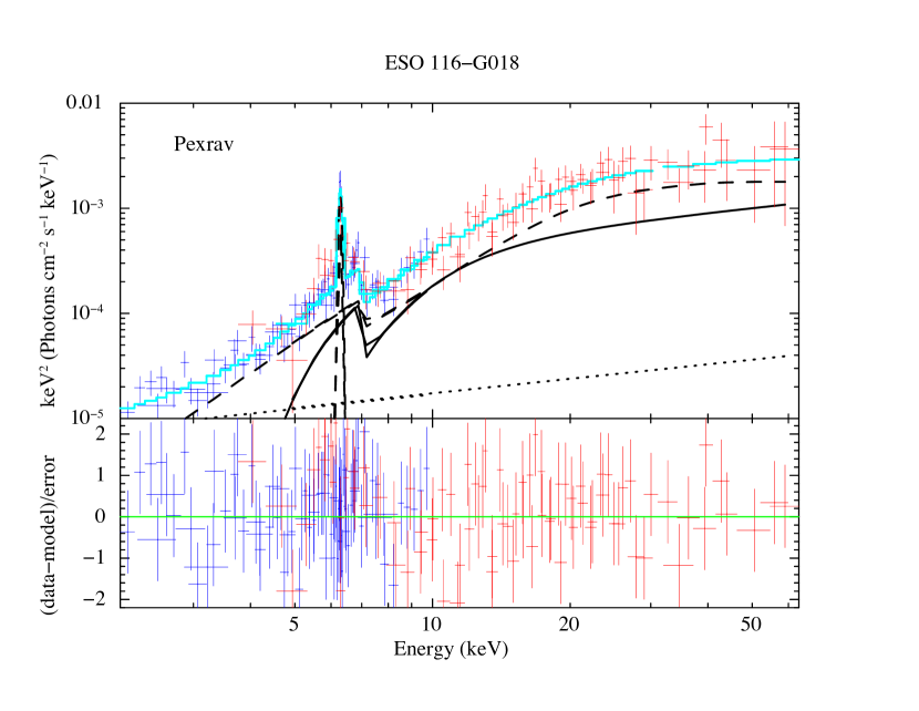
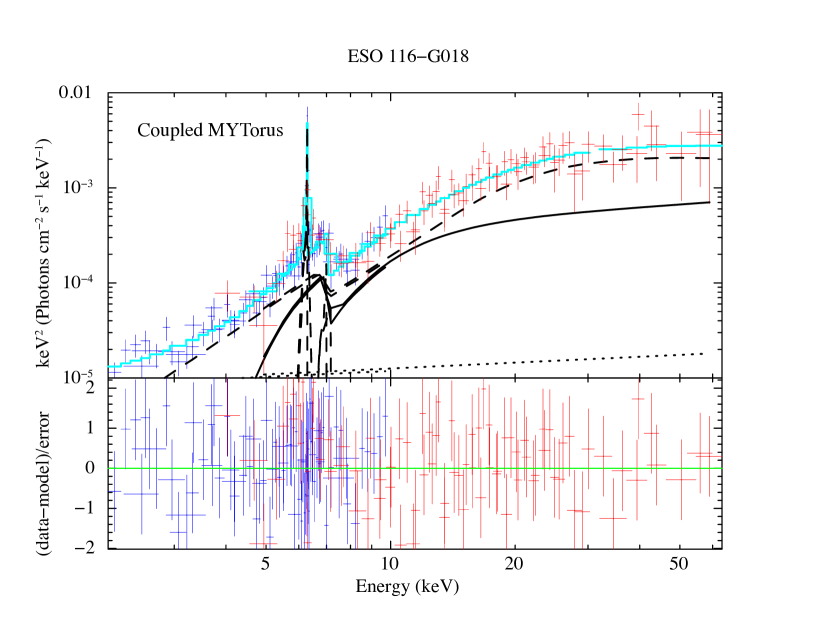
Figure 3.— Unfolded XMM-Newton and NuSTAR spectra of ESO 116-G018 fitted with model B (left panel) and ‘coupled’ MYTorus model (right panel). The XMM-Newton data are plotted in blue, while the NuSTAR data are plotted in red. The best-fit models prediction is plotted as a cyan solid line. The single components of the model are plotted in black with different line styles, i.e., the absorbed intrinsic continuum as a solid line, the reprocessed component and Fe K$\alpha$ line as a dashed line and the scattered component as a dotted line.

3.2.3 MYTorus in ‘coupled’ configuration

In ‘coupled’ mode, both the inclination angle and the column density are tied among the three components: MYTZ, MYTS, MYTL. In this configuration, the column density is the torus equatorial one, and the “line-of-sight” column density is N_H,l.o.s = N_H,eq $\times$ $\rm(1-4\times cos(\theta_{obs})^{2})^{1/2}$ (Murphy & Yaqoob, 2009).

The best-fit photon index for ‘coupled’ MYTorus model is $\Gamma$ = 1.79${}_{-0.12}^{+0.11}$; the photon indices of the Compton-scattered continuum and of the fluorescent emission-lines component are tied to that of direct continuum. The equatorial column density is N_H,eq = 5.31${}_{-2.71}^{+2.34}$ $\times$ $10^{24}$ cm^-2 and the inclination angle is $\theta_{\rm obs}$ = 60.70${}_{-0.40}^{+0.82}$^∘, such that the “line-of-sight” column densities are N_H,Z = 2.60${}_{-1.36}^{+1.19}$ $\times$ $10^{24}$ cm^-2.

While the best-fit statistics of the ‘coupled’ model is good ($\chi^{2}_{\nu}$ = 140/161 = 0.87), the geometrical scenario which the model presents is physically unlikely, since we measure $\theta_{\rm obs}$= 60.70^∘ $\sim$60^∘ = $\theta_{\rm tor}$, i.e., the AGN would be observed through the brink of the torus. Such a result also affects the reliability of the column density measurement, since N_H,Z is a parameter highly dependent on $\theta_{\rm obs}$, particularly when $\theta_{\rm obs}$ gets close to $\theta_{\rm tor}$. To further investigate the physical and geometrical properties of ESO 116-G018, we, therefore, try to apply MYTorus in a different configuration, which allows one to disentangle the inclination angle and column density between the direct continuum and the reprocessed component.

3.2.4 MYTorus in ‘decoupled’ configuration

In ‘decoupled’ configuration (Yaqoob, 2012), the direct continuum and the Compton scattered component can in principle have different inclination angle and column density values. Since the direct continuum is a pure “line-of-sight” quality, which is independent on observation angle, the inclination angle of the direct continuum is fixed to $\theta_{\rm obs,Z}$ = 90^∘, such that the column density of the direct continuum models the “line-of-sight” column density, N_H,Z. The inclination angle of the Compton-scattered continuum and fluorescent lines is instead set to be either $\theta_{\rm obs,S,L}$ = 0^∘ (face on) or $\theta_{\rm obs,S,L}$ = 90^∘ (edge on), modeling a “back-side” reflection-dominated scenario or a “near-side” Compton scattered component-dominated scenario, respectively. In this configuration, the column density of the Compton scattered component and fluorescent emission-lines component parameterizes the “global averaged” column density of the torus, N_H,S, which can significantly differ from the “line-of-sight” column density in an inhomogeneous, patchy, torus (see Yaqoob, 2012, for more details). Therefore, MYTorus in ‘decoupled’ configuration can be used to model a more realistic distribution of the obscuring material. We point out that the fluorescent emission lines component and Compton scattered component are still coupled since they are expected to be originated from the same process.

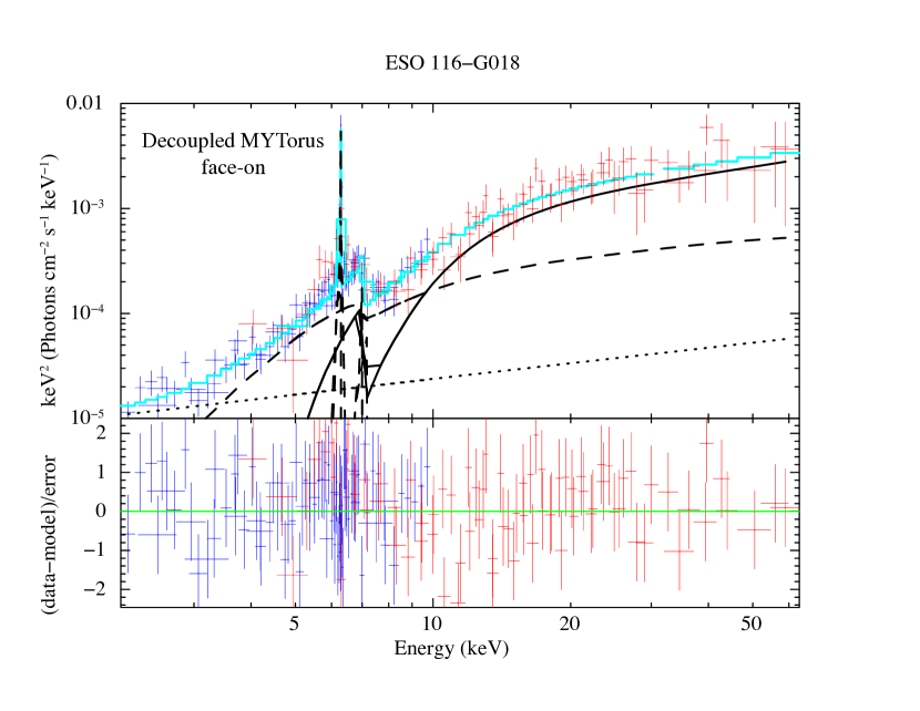
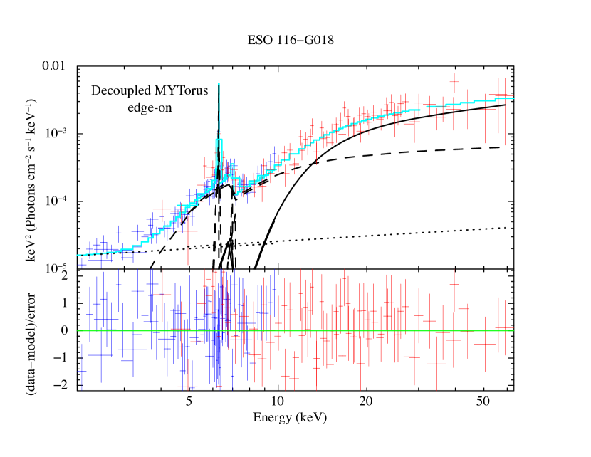
Figure 4.— Unfolded XMM-Newton and NuSTAR spectra of ESO 116-G018 fitted with ‘decoupled’ MYTorus “face-on” model (left panel) and ‘decoupled’ MYTorus “edge-on” model (right panel). The XMM-Newton data are plotted in blue, while the NuSTAR data are plotted in red. The best-fit models prediction is plotted as a cyan solid line. The single components of the model are plotted in black with different line styles, i.e., the absorbed intrinsic continuum as a solid line, the reprocessed component and Fe K$\alpha$ line as a dashed line and the scattered component as a dotted line.

The best-fit photon indices are $\Gamma_{\rm\theta,S=0}$ = 1.51${}_{-0.11}^{+0.37}$ and $\Gamma_{\rm\theta,S=90}$ = 1.74${}_{-0.34}^{+0.40}$ for “face on” and “edge on” modes respectively. The “line-of-sight” column densities are N_H,Z,θ,S=0 = 1.46${}_{-0.30}^{+0.57}$ $\times$ $10^{24}$ cm^-2 and N_H,Z,θ,S=90 = 2.58${}_{-0.83}^{+1.21}$ $\times$ $10^{24}$ cm^-2. The “global average” column densities are N_H,S,θ,S=0 = 0.43${}_{-0.13}^{+0.21}$ $\times$ 10²⁴ cm^-2 and N_H,S,θ,S=90 = 0.38${}_{-0.08}^{+0.11}$ $\times$ $10^{24}$ cm^-2. The “global average” column densities are $\sim$15% and 29% of the “line-of-sight” column densities for “edge-on” and “face-on” configurations, respectively, which suggests a patchy torus in ESO 116-G018. We present the unfolded NuSTAR and XMM-Newton spectra of ESO 116-G018 using the ‘decoupled’ MYTorus model in “face on” and “edge on” configuration in Fig. 4.

In conclusion, the best-fit results of the MYTorus model in both ‘coupled’ MYTorus model and ‘decoupled’ MYTorus model in “edge on” configuration confirm that ESO 116-G018 is a bona fide CT-AGN at $>$3 $\sigma$ confidence. While MYTorus is effective in modeling the X-ray spectra of heavily obscured AGN, the ‘coupled’ mode assumes a fixed torus opening angle ($\theta_{\rm Tor}$=60^∘, i.e., a covering factor $f_{c}$ = cos $\theta_{\rm Tor}$ = 0.5), limiting the model to a single torus geometry and the ‘decoupled’ mode fails to directly parameterize the geometrical properties of the obscuring material. To complement our analysis, we, therefore, model the ESO 116-G018 spectrum using the recently published borus02 model (Baloković et al., 2018), an updated version of the so-called BNtorus model (Brightman & Nandra, 2011).

3.2.5 BORUS02

The model is composed of a reprocessed component (including the Compton scattered component and fluorescent lines) and an absorbed intrinsic continuum, described by a cut-off power-law, multiplied by a “line-of-sight” absorbing component, zphabs$\times$cabs. Although the $cabs$ model simply assumes a constant Compton scattering cross section equal to the Thomson cross section, which is in principle energy-dependent and only valid below $\sim$10 keV, the difference between such a model and MYTZ is insignificant below $100$ keV in our case, where N_H,Z $\sim 2.6$ $\times$ $10^{24}$ cm^-2 (more details are available in the MYTorus manual). In borus02 the torus covering factor can vary in range of $f_{c}$ = [0.1–1], corresponding to a torus opening angle $\theta_{\rm Tor}$ = [0–84]^∘. The observing angle ranges from $\theta_{\rm Tor}$ $\sim$[18–87]^∘.

The borus02 model is used in the following XSPEC configuration:

$$ModelD= constant_{1}*phabs*(borus+zphabs*cabs$$ (4)

$$*cutoffpl+constant_{2}*cutoffpl)$$

where borus is the reprocessed component in borus02.

The best-fit photon index is $\Gamma$ = 1.80${}_{-0.06}^{+0.06}$; the “line-of-sight” column density is N_H,Z = 2.60${}_{-0.14}^{+0.16}$ $\times$ $10^{24}$ cm^-2; the column density of the torus is N_H,S = 0.52${}_{-0.06}^{+0.10}$ $\times~{}10^{24}$ cm^-2: in good agreement with the ‘decoupled’ MYTorus model in “edge-on” configuration. The half-opening angle of the torus is $\theta\rm_{tor}$ = 81.69${}_{-0.30}^{+0.88}$^∘, thus the torus covering factor is $f_{c}$ = cos($\theta\rm_{tor}$) = 0.14${}_{-0.01}^{+0.01}$. The inclination angle between the observer and the torus axis is $\theta\rm_{obs}$ = 84.78${}_{-0.88}^{+0.86}$. The unfolded NuSTAR and XMM-Newton spectra of ESO 116-G018 fitted with borus02 model is presented in Fig.  5.

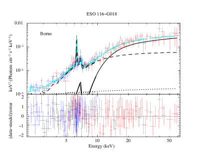
Figure 5.— Unfolded XMM-Newton and NuSTAR spectra of ESO 116-G018 fitted with the borus02 model. The XMM-Newton data are plotted in blue, while the NuSTAR data are plotted in red. The best-fit models prediction is plotted as a cyan solid line. The single components of the model are plotted in black with different line styles, i.e., “line-of-sight” continuum as a solid line, reprocessed component as a dashed line and the scattered component as a dotted line.

To conclude, the self-consistent, physically motivated models of MYTorus and borus02 give a better characterization of the X-ray spectrum than the phenomenological model and the pexrav model, and confirm ESO 116-G018 to be a CT-AGN at $>$3 $\sigma$ confidence. In addition, both the MYTorus model in ‘decoupled’ configuration and borus02 display a significant difference between the “line-of-sight” column density and the column density of the torus, suggesting a patchy distribution of the obscuring matter. The other physical properties of interest will be discussed in Section 4.

3.3. Summary of the spectral analyzing results

In Section 3.1, we first fitted the combined high-quality XMM-Newton-NuSTAR spectra of ESO 116-G018 using the phenomenological model A, finding that only an absorbed power-law is difficult to characterize the Compton hump in $\sim$10–40 keV. We thus added a reflection component pexrav to the model B to characterize the Compton hump: we obtained a significantly improved statistic, but the lack of self-consistency motivated us to explore more realistic models, i.e., MYTorus and borus02, where the structure of the obscuring matter is a torus rather than a slab, like in pexrav. In Section 3.2.2, we first tested the ‘coupled’ MYTorus model, which gave an unlikely geometrical scenario, i.e., the accreting SMBH would be observed through the brink of the torus. Therefore, we adopted the MYTorus model configuration that assumes a more general geometry, by disentangling the direct continuum and the reprocessed component, and we then fitted the spectrum with the so-called ‘decoupled’ MYTorus model. This model gave a more reasonable result: however the obscuring material geometrical properties, i.e., the covering factor $f_{c}$ and observing angle $\theta_{\rm obs}$ cannot be directly derived using MYTorus in ‘decoupled’ configuration. Thus, we finally tested the recently published borus02 model, which gives the best statistics and allows one to measure $f_{c}$ and $\theta_{\rm obs}$.

Based on both the fit statistics and the reliability of the best-fit parameters, we believe that borus02 provides the best-fit model for ESO 116-G018 in the 2–70 keV band. In fact, while all the models used in our analysis have good fit statistics ($\chi^{2}_{\nu}$ $\sim$0.87–1.02), models other than borus02 are limited by the assumptions required to use them or have notably different physical interpretations. For example, the pexrav model and ‘coupled’ MYTorus model indicate that the spectrum is dominated by the reprocessed component, while the ‘decoupled’ MYTorus model and borus02 model suggest that the direct continuum dominate the spectrum especially at energy $E$ $>$10 keV. Such a discrepancy is also observed in other parameters, e.g., the intrinsic luminosity, which will be further discussed in Section 4.4. However, it is worth pointing out that in reprocessing-dominated models, such as pexrav  the reprocessed component is not obscured, while in ‘coupled’ MYTorus model, the reprocessed component is obscured by the dust and gas with the same column density as the “line-of-sight” one: both scenarios are unlikely to exactly characterize the real distribution of obscuring material, which has been shown to be clumpy, rather than uniformly distributed (see, e.g., Krolik & Begelman, 1988; Jaffe et al., 2004; Tristram et al., 2007; Nenkova et al., 2008; Hönig & Kishimoto, 2010; Stalevski et al., 2012). Indeed, the significant difference between the “line-of-sight” column density and the ‘global average’ column density of the torus observed in the ‘decoupled’ MYTorus model and in the borus02 model best-fits support a clumpy, patchy torus scenario for ESO 116-G018.

Regardless of the geometrical configuration of the obscuring material, both self-consistent, physically motivated models, MYTorus and borus02, confirm the Compton-thickness of ESO 116-G018 at $>$3 $\sigma$ confidence level. Furthermore, the borus02 model provides excellent constraints on the geometrical properties of the obscuring torus: the covering factor is $f_{c}$ = [0.13–0.15] and we are observing the source “edge-on”.

4. Discussion and Conclusions

In this work, we report the results of the 2–70 keV spectral analysis of ESO 116-G018, a nearby Seyfert 2 galaxy, observed quasi-simultaneously by NuSTAR (45 ks) and XMM-Newton (58 ks), and we establish for the first time that the source is a bona fide Compton-thick AGN. As discussed in Section 3.3, the best-fit model for ESO 116-G018 is borus02 (Baloković et al., 2018), which gives a “line-of-sight” column density of N_H,Z = [2.46–2.76] $\times$ $10^{24}$ cm^-2. We also find that the best-fit results of ‘decoupled’ MYTorus model in “edge on” configuration (Murphy & Yaqoob, 2009) are in excellent agreement with those of borus02 model. In the rest of the paper, we will use the borus02 model best-fit results.

4.1. Comparison with previous results

ESO 116-G018 was found to be a CT-AGN candidate by Marchesi et al. (2017a), using a joint Chandra-Swift/BAT spectra fitted with the MYTorus model in ‘coupled’ configuration where the inclination angle is fixed to be $\theta\rm_{obs}$=90^∘: they found a best-fit photon index, $\Gamma$ = 1.86${}_{-0.48}^{+0.51}$, in good agreement with the one measured in this work and a best-fit column density of N_H = 0.95${}_{-0.40}^{+0.46}$ $\times$ $10^{24}$ cm^-2, with $\chi^{2}$/d.o.f. = 17/14. Such a large uncertainty has been significantly improved by the high-quality data of the combined NuSTAR-XMM-Newton observations, which is potential the best combination of observatories to study the CT-AGNs in X-ray band.

4.2. Equivalent width of the iron K$\alpha$ line

We are able to place strong constraints on the Fe K$\alpha$ line equivalent width (EW) of ESO 116-G018, due to the excellent count statistics provided by NuSTAR and XMM-Newton in the 5–8 keV band, with a significant improvement with respect to Marchesi et al. (2017a). We use the task eqwidth in XSPEC to measure the equivalent width EW_phe = 0.93${}_{-0.15}^{+0.15}$ keV and EW_pex = 0.85${}_{-0.13}^{+0.15}$ keV in models A and B, respectively.

To measure the Fe K$\alpha$ line EW with MYTorus we use the approach described in Yaqoob et al. (2015). We therefore first measure the continuum flux, without including the emission line, at E_Kα = 6.4 keV. We then compute the flux of the fluorescent lines component in the energy range E = [0.95 E_Kα–1.05 E_Kα], i.e., between 6.08 and 6.72 keV, rest-frame. EW is then computed by multiplying by (1 + z) the ratio between the fluorescent line flux and the monochromatic continuum flux. We obtain EW_coupl = 0.78${}_{-0.13}^{+0.09}$ keV, EW_decoupl,θ=0 = 0.90${}_{-0.13}^{+0.10}$ keV and EW_{decoupl,θ=90} = 0.85${}_{-0.12}^{+0.12}$ keV. All MYTorus equivalent width values are in good agreement with the ones obtained by phenomenological model and pexrav model: furthermore, in all the models the measured Iron line EW value is typical of a CT-AGN ($\sim$1 keV; see, e.g., Fig. 8 in Murphy & Yaqoob, 2009).

4.3. Intrinsic luminosity

We report the 2–10 keV and 10–40 keV intrinsic luminosity in Table 2. Notably, the intrinsic luminosities derived from model B and the ‘coupled’ MYTorus model are $\sim$12–25 times smaller than those derived using borus02 model the ‘decoupled’ MYTorus “edge-on” model. As discussed in Section 3.3, this is due to the fact that model B and ‘coupled’ MYTorus model are reprocessed-component-dominated, while borus02 and the ‘decoupled’ MYTorus “edge-on” model are direct-continuum-dominated (at least at energies E$>$10 keV). As already discussed in the previous sections, based on the statistics and reliability of parameters, we favor the borus02 and MYTorus decoupled “edge-on” solutions. The 2–10 keV and 10–40 keV intrinsic luminosity from the best-fit model are L_int,2-10 = 1.68${}_{-0.19}^{+0.18}$ $\times$ 10⁴³ erg s^-1 and L_int,10-40 = 1.86${}_{-0.21}^{+0.21}$ $\times$ 10⁴³ erg s^-1, respectively. This luminosity is compatible with the knee of the luminosity function of AGN in the local Universe (Ajello et al., 2012), showing that ESO 116-G018 is an average-luminosity AGN.

The intrinsic X-ray luminosity can be derived indirectly from the luminosities measured at other wavelengths, such as the mid-infrared (MIR, 3–20 $\mu$m; see, e.g., Elvis et al., 1978). The MIR flux of ESO 116-G018 is F_12μm = 0.175${}_{-0.003}^{+0.002}$ Jy (Wright et al., 2010), and the corresponding luminosity is L_12μm = 3.34${}_{-0.05}^{+0.04}$ $\times$ 10⁴³ erg s^-1. Applying the MIR-X-ray correlation in Asmus et al. (2015) to the MIR luminosity, we obtain the 2–10 keV luminosity to be L_int,2-10,MIR = 0.42${}_{-0.10}^{+0.12}$ $\times$ 10⁴³ erg s^-1. The 2–10 keV intrinsic luminosity derived from MIR luminosity is slightly less than our best-fit one. This may be due to the fact that the covering factor of ESO 116-G018 is indeed small (see Section 4.5), which leads to a relative small infrared luminosity.

4.4. Bolometric luminosity and mass of SMBH

The AGN bolometric luminosity is the measurement of the total AGN emission over the whole electromagnetic spectrum, and several bolometric corrections measurements to infer the bolometric luminosity from the X-ray one have been reported in the literature (see, e.g., Elvis et al., 1994; Marconi et al., 2004; Lusso et al., 2012; Brightman et al., 2017). In Section 3, we measured the intrinsic luminosity of ESO 116-G018 between 2–10 keV which is L${}_{\rm int,2-10\,keV}$ = 1.68${}_{-0.19}^{+0.18}$ $\times$ 10⁴³ erg s^-1 using our best-fit borus02 model. Applying the bolometric correction of Marconi et al. (2004, Equation 21), we obtain the bolometric luminosity of ESO 116-G018, which is L_bol = 2.99${}_{-0.42}^{+0.42}$ $\times$ 10⁴⁴ erg s^-1.

Recently, Brightman et al. (2017) measured the X-ray bolometric correction factors, $\kappa_{\rm Bol}$ $\equiv$L_bol/L_obs,8-24, where L_obs,8-24 is the observed luminosity in 8–24 keV, for CT AGNs. ESO 116-G018 8–24 keV observed luminosity is L_obs,8-24 = 1.23${}_{-0.12}^{+0.14}$ $\times$ 10⁴² erg s^-1, such that the bolometric luminosity from the prediction of Brightman et al. (2017) is L_bol = 3.22${}_{-2.11}^{+6.11}$ $\times$ 10⁴⁴ erg s^-1, in excellent agreement with our results measured using the Marconi et al. (2004) bolometric correction.

The Eddington ratio is a measurement of the SMBH accretion efficiency, and is defined as $\lambda_{\rm Edd}$ = $L_{\rm bol}/L_{\rm Edd}$, i.e., the ratio of bolometric luminosity, $L_{\rm bol}$, to the so-called Eddington luminosity, $L_{\rm Edd}$ = 4$\pi$GM_BHm_pc/$\sigma_{T}$, where M_BH is the SMBH mass and m_p is the mass of proton. Combining the bolometric luminosity, L_bol, and the typical Eddington ratio of AGNs in local universe ($\lambda$ $\sim$0.1; see, e.g., Marconi et al., 2004), one can estimate the mass of the center engine in ESO 116-G018, which is M_BH = $L_{\rm bol}$/(4$\pi$Gm_pc$\lambda_{\rm Edd}$/$\sigma_{T}$) and we obtain log (M_BH/M_☉) $\sim$7.4, which is in agreement with the typical mass of SMBH: log (M_BH/M_☉) $\sim$6.0–9.8 (see, e.g., Woo & Urry, 2002).

4.5. Covering factor

The self-consistency of the reprocessed components in borus02 model provides one with the possibility to directly derive the geometrical properties of the obscuring material. In Section 3.2.5, we measured the covering factor of the torus in ESO 116-G018 using borus02, and we found that a low-covering factor solution ($f_{c}$ = 0.14${}_{-0.01}^{+0.01}$) is preferred. It is worth to note that this low covering factor could be explained both with a geometrically thin torus or with the fact that the torus is patchy, which is supported by the observed discrepancy between the “line-of-sight” column density and the ‘global average’ column density of the torus.

The optical/UV disk emission re-processed by the torus in the infrared (IR) can also provide interesting constraints on the source geometry. The ratio of the torus luminosity to the AGN luminosity can be thus be interpreted as the fraction of the sky obscured by the ‘torus-like’ material, and the covering factor can be measured with the equation $f_{c}$ $\equiv$L_tor/L_AGN = L_IR/L_Bol (Stalevski et al., 2016). Yamada et al. (2013) measured the IR (8–1000 $\mu$m) luminosity of ESO 116-G018, which is L_IR = 1.3 $\times$ 10⁴⁴ erg s^-1, using the IRSA (Neugebauer et al., 1984) 12, 25, 60 and 100 $\mu$m observations. Based on their measurement, and using the bolometric luminosity estimated from our best-fit model discussed in Section 4.4, the IR covering factor of the torus is $f_{c}$ = [0.38–0.51]. However, ESO 116-G018 is classified as a composite galaxy (Yamada et al., 2013), i.e., the galaxy has both star-forming and AGN activity signatures, thus the IR luminosity is constituted of not only the AGN contribution but also a significant fraction of the polycyclic aromatic hydrocarbon (PAH) emission in star-forming process, suggesting that the covering factor of the torus of ESO 116-G018 should be smaller than that derived with the technique discussed above: the constraints on the geometrical property of the torus from the infrared study are thus in line with those obtained from our measurement in X-ray.

4.6. Conclusion

We find a significant difference between the best-fit results of the phenomenological model and pexrav model, and the best-fit results of the self-consistent, physically motivated models. Such a difference is also found in NGC 1358 (Zhao et al. 2018 accepted). In addition, Marchesi et al. (2018) re-examined the distribution of the column density of a sampled AGNs in local universe accompanied with NuSTAR data, finding an overestimation of the column density than the one measured with Swift-BAT data probably due to the low-quality of the spectra. Since most of the AGNs are modeled with phenomenological model and non-self-consistent, physically motivated model in the previous analysis, the observed distribution of AGN will vary if self-consistent, physically motivated models are widely adopted. However, it is worth noting that the self-consistent, physically motivated models, i.e., MYTorus and borus02, require high-quality data in broadband, therefore, as we show in this work and the work discussed above, the physically motivated model complemented with the combined NuSTAR and XMM-Newton analysis will be an ideal method to study the physics of heavily obscured AGNs.

References

- Aird et al. (2015) Aird, J., Alexander, D. M., Ballantyne, D. R., et al. 2015, ApJ, 815, 66
- Ajello et al. (2012) Ajello, M., Alexander, D. M., Greiner, J., et al. 2012, The Astrophysical Journal, 749, 21
- Ajello et al. (2008) Ajello, M., Greiner, J., Sato, G., et al. 2008, The Astrophysical Journal, 689, 666
- Alexander et al. (2003) Alexander, D. M., Bauer, F. E., Brandt, W. N., et al. 2003, The Astronomical Journal, 126, 539
- Almeida & Ricci (2017) Almeida, C. R. & Ricci, C. 2017, Nature Astronomy, 1, 679
- Anders & Grevesse (1989) Anders, E. & Grevesse, N. 1989, Geochimica et Cosmochimica Acta, 53, 197
- Annuar et al. (2015) Annuar, A., Gandhi, P., Alexander, D. M., et al. 2015, The Astrophysical Journal, 815, 36
- Arnaud (1996) Arnaud, K. A. 1996, Astronomical Data Analysis Software and Systems V, 101, 17
- Asmus et al. (2015) Asmus, D., Gandhi, P., Hönig, S. F., Smette, A., & Duschl, W. J. 2015, Monthly Notices of the Royal Astronomical Society, 454, 766
- Baloković et al. (2018) Baloković, M., Brightman, M., Harrison, F. A., et al. 2018, The Astrophysical Journal, 854, 42
- Baloković et al. (2014) Baloković, M., Comastri, A., Harrison, F. A., et al. 2014, The Astrophysical Journal, 794, 111
- Barthelmy et al. (2005) Barthelmy, S. D., Barbier, L. M., Cummings, J. R., et al. 2005, Space Science Reviews, 120, 143
- Brightman et al. (2017) Brightman, M., Baloković, M., Ballantyne, D. R., et al. 2017, The Astrophysical Journal, 844, 10
- Brightman & Nandra (2011) Brightman, M. & Nandra, K. 2011, Monthly Notices of the Royal Astronomical Society, 413, 1206
- Buchner et al. (2015) Buchner, J., Georgakakis, A., Nandra, K., et al. 2015, The Astrophysical Journal, 802, 89
- Burlon et al. (2011) Burlon, D., Ajello, M., Greiner, J., et al. 2011, The Astrophysical Journal, 728, 58
- de Grijp et al. (1992) de Grijp, M. H. K., Keel, W. C., Miley, G. K., Goudfrooij, P., & Lub, J. 1992, A&AS, 96, 389
- Elvis et al. (1978) Elvis, M., Maccacaro, T., Wilson, A. S., et al. 1978, Monthly Notices of the Royal Astronomical Society, 183, 129
- Elvis et al. (1994) Elvis, M., Wilkes, B. J., McDowell, J. C., et al. 1994, ApJS, 95, 1
- Furui et al. (2016) Furui, S., Fukazawa, Y., Odaka, H., et al. 2016, The Astrophysical Journal, 818, 164
- Gandhi & Fabian (2003) Gandhi, P. & Fabian, A. C. 2003, Monthly Notices of the Royal Astronomical Society, 339, 1095
- Georgantopoulos et al. (2013) Georgantopoulos, I., Comastri, A., Vignali, C., et al. 2013, A&A, 555, A43
- Gilli et al. (2007) Gilli, R., Comastri, A., & Hasinger, G. 2007, A&A, 463, 79
- Goulding et al. (2011) Goulding, A. D., Alexander, D. M., Mullaney, J. R., et al. 2011, Monthly Notices of the Royal Astronomical Society, 411, 1231
- Harrison et al. (2016) Harrison, F. A., Aird, J., Civano, F., et al. 2016, The Astrophysical Journal, 831, 185
- Harrison et al. (2013) Harrison, F. A., Craig, W. W., Christensen, F. E., et al. 2013, The Astrophysical Journal, 770, 103
- Hickox & Markevitch (2006) Hickox, R. C. & Markevitch, M. 2006, The Astrophysical Journal, 645, 95
- Hönig & Kishimoto (2010) Hönig, S. F. & Kishimoto, M. 2010, A&A, 523, A27
- Ikeda et al. (2009) Ikeda, S., Awaki, H., & Terashima, Y. 2009, The Astrophysical Journal, 692, 608
- Jaffe et al. (2004) Jaffe, W., Meisenheimer, K., Röttgering, H. J. A., et al. 2004, Nature, 429, 47 EP
- Jansen et al. (2001) Jansen, F., Lumb, D., Altieri, B., et al. 2001, A&A, 365, L1
- Kalberla et al. (2005) Kalberla, P. M. W., Burton, W. B., Hartmann, Dap, et al. 2005, A&A, 440, 775
- Koss et al. (2016) Koss, M. J., Assef, R., Baloković, M., et al. 2016, The Astrophysical Journal, 825, 85
- Krolik & Begelman (1988) Krolik, J. H. & Begelman, M. C. 1988, Astrophysical Journal, 329, 702
- Lanzuisi et al. (2015) Lanzuisi, G., Ranalli, P., Georgantopoulos, I., et al. 2015, A&A, 573, A137
- Liu & Li (2014) Liu, Y. & Li, X. 2014, The Astrophysical Journal, 787, 52
- Lusso et al. (2012) Lusso, E., Comastri, A., Simmons, B. D., et al. 2012, Monthly Notices of the Royal Astronomical Society, 425, 623
- Magdziarz & Zdziarski (1995) Magdziarz, P. & Zdziarski, A. A. 1995, Monthly Notices of the Royal Astronomical Society, 273, 837
- Marchesi et al. (2017a) Marchesi, S., Ajello, M., Comastri, A., et al. 2017a, The Astrophysical Journal, 836, 116
- Marchesi et al. (2018) Marchesi, S., Ajello, M., Marcotulli, L., et al. 2018, The Astrophysical Journal, 854, 49
- Marchesi et al. (2017b) Marchesi, S., Tremblay, L., Ajello, M., et al. 2017b, The Astrophysical Journal, 848, 53
- Marconi et al. (2004) Marconi, A., Risaliti, G., Gilli, R., et al. 2004, Monthly Notices of the Royal Astronomical Society, 351, 169
- Matt & Fabian (1994) Matt, G. & Fabian, A. C. 1994, Monthly Notices of the Royal Astronomical Society, 267, 187
- Murphy & Yaqoob (2009) Murphy, K. D. & Yaqoob, T. 2009, Monthly Notices of the Royal Astronomical Society, 397, 1549
- Nenkova et al. (2008) Nenkova, M., Sirocky, M. M., Ivezić, Ž., & Elitzur, M. 2008, The Astrophysical Journal, 685, 147
- Neugebauer et al. (1984) Neugebauer, G., Habing, H. J., van Duinen, R., et al. 1984, ApJ, 278, L1
- Puccetti et al. (2014) Puccetti, S., Comastri, A., Fiore, F., et al. 2014, The Astrophysical Journal, 793, 26
- Ricci et al. (2015) Ricci, C., Ueda, Y., Koss, M. J., et al. 2015, The Astrophysical Journal Letters, 815, L13
- Ricci et al. (2011) Ricci, C., Walter, R., Courvoisier, T. J.-L., & Paltani, S. 2011, A&A, 532, A102
- Risaliti et al. (1999) Risaliti, G., Maiolino, R., & Salvati, M. 1999, The Astrophysical Journal, 522, 157
- Stalevski et al. (2012) Stalevski, M., Fritz, J., Baes, M., Nakos, T., & Popović, L. Č. 2012, Monthly Notices of the Royal Astronomical Society, 420, 2756
- Stalevski et al. (2016) Stalevski, M., Ricci, C., Ueda, Y., et al. 2016, Monthly Notices of the Royal Astronomical Society, 458, 2288
- Strüder et al. (2001) Strüder, L., Briel, U., Dennerl, K., et al. 2001, A&A, 365, L18
- Treister et al. (2009) Treister, E., Urry, C. M., & Virani, S. 2009, The Astrophysical Journal, 696, 110
- Tristram et al. (2007) Tristram, K. R. W., Meisenheimer, K., Jaffe, W., et al. 2007, A&A, 474, 837
- Turner et al. (2001) Turner, M. J. L., Abbey, A., Arnaud, M., et al. 2001, A&A, 365, L27
- Ueda et al. (2014) Ueda, Y., Akiyama, M., Hasinger, G., Miyaji, T., & Watson, M. G. 2014, The Astrophysical Journal, 786, 104
- Ursini et al. (2018) Ursini, F., Bassani, L., Panessa, F., et al. 2018, Monthly Notices of the Royal Astronomical Society, 474, 5684
- Verner et al. (1996) Verner, D., Ferland, G., Korista, K., & Yakovlev, D. 1996, Astrophysical Journal, 465, 487
- Winkler et al. (2003) Winkler, C., T. J.-L. Courvoisier, Di Cocco, G., et al. 2003, A&A, 411, L1
- Woo & Urry (2002) Woo, J.-H. & Urry, C. M. 2002, The Astrophysical Journal, 579, 530
- Worsley et al. (2005) Worsley, M. A., Fabian, A. C., Bauer, F. E., et al. 2005, Monthly Notices of the Royal Astronomical Society, 357, 1281
- Wright et al. (2010) Wright, E. L., Eisenhardt, P. R. M., Mainzer, A. K., et al. 2010, The Astronomical Journal, 140, 1868
- Yamada et al. (2013) Yamada, R., Oyabu, S., Kaneda, H., et al. 2013, Publications of the Astronomical Society of Japan, 65, 103
- Yaqoob (2012) Yaqoob, T. 2012, Monthly Notices of the Royal Astronomical Society, 423, 3360
- Yaqoob et al. (2015) Yaqoob, T., Tatum, M. M., Scholtes, A., Gottlieb, A., & Turner, T. J. 2015, Monthly Notices of the Royal Astronomical Society, 454, 973