Observation of parity-time symmetry breaking in a single spin system

Abstract

A fundamental axiom of quantum mechanics requires the Hamiltonians to be Hermitian which guarantees real eigen-energies and probability conservation. However, a class of non-Hermitian Hamiltonians with Parity-Time ($\mathcal{PT}$) symmetry can still display entirely real spectra PRL_Bender_1998 . The Hermiticity requirement may be replaced by $\mathcal{PT}$ symmetry to develop an alternative formulation of quantum mechanicsPRL_Bender_2002 ; RPP_Bender . A series of experiments have been carried out with classical systems including opticsNP_Ruter , electronicsPRL_N_Bender ; Nature_Assawaworrarit ; NC_Choi , microwavesPRL_Bittner , mechanicsAJP_Bender and acousticsPRX_Zhu ; NC_Popa ; NC_Fleury . However, there are few experiments to investigate $\mathcal{PT}$ symmetric physics in quantum systems. Here we report the first observation of the $\mathcal{PT}$ symmetry breaking in a single spin system. We have developed a novel method to dilate a general $\mathcal{PT}$ symmetric Hamiltonian into a Hermitian one, which can be realized in a practical quantum system. Then the state evolutions under $\mathcal{PT}$ symmetric Hamiltonians, which range from $\mathcal{PT}$ symmetric unbroken to broken regions, have been experimentally observed with a single nitrogen-vacancy (NV) center in diamond. Due to the universality of the dilation method, our result opens a door for further exploiting and understanding the physical properties of $\mathcal{PT}$ symmetric Hamiltonian in quantum systems.

In quantum mechanics, the real energies of a system are guaranteed by a fundamental axiom associated with the Hermiticity of physical observables. However, a class of non-Hermitian Hamiltonians satisfying $\mathcal{PT}$ symmetry can still exhibit real eigenenergiesPRL_Bender_1998 . In principle, wider range of systems can be described by $\mathcal{PT}$ symmetric Hamiltonians comparing to Hermitian ones. A Hamiltonian $H$ is considered to be $\mathcal{PT}$ symmetric if $[\mathcal{PT},H]=0$, where $\mathcal{P}$ and $\mathcal{T}$ denote the parity and time-reversal operators, respectively. A sufficient condition for a $\mathcal{PT}$ symmetric Hamiltonian $H$ to exhibit entire real eigenvalues is that $H$ corresponds to the region of unbroken $\mathcal{PT}$ symmetry, where any eigenfunction of $H$ is simultaneously an eigenfunction of the $\mathcal{PT}$ operator. Otherwise, if the $\mathcal{PT}$ symmetric Hamiltonian $H$ and the $\mathcal{PT}$ operator possess different eigenfunctions, $H$ corresponds to the region of broken $\mathcal{PT}$ symmetry. A Hamiltonian $H$ with a broken $\mathcal{PT}$ symmetry is typically associated with the presence of complex eigenenergies. An alternative formulation of quantum mechanics can be established in which the axiom of Hermiticity is replaced by the condition of $\mathcal{PT}$ symmetryPRL_Bender_2002 ; RPP_Bender .

The rich physics associated with $\mathcal{PT}$ symmetric Hamiltonian have aroused considerable experimental interestNP_El_Ganainy . A series of experiments have been performed with classical approaches. The optical analog of $\mathcal{PT}$ symmetric quantum mechanics was firstly proposedNP_Ruter , then the concept was quickly extended to other systems, such as electronicsPRL_N_Bender ; Nature_Assawaworrarit ; NC_Choi , microwavesPRL_Bittner , mechanicsAJP_Bender , acousticsPRX_Zhu ; NC_Popa ; NC_Fleury , and optical systems with atomic mediaPRL_Hang ; NP_Peng_2016 ; PRL_Zhang . In particular, the experimental research on $\mathcal{PT}$ symmetric classical optical systems has been honored as a most important accomplishment in the past decadeNP_Cham and has stimulated many applications such as unidirectional light transportScience_Feng_2011 ; NP_Peng_2014 and single-mode lasersScience_Feng_2014 ; Science_Hodaei . As a contrast, it is still of challenge to experimentally investigate $\mathcal{PT}$ symmetric Hamiltonian related physics in quantum systems. This is because that experimental quantum systems are governed by Hermitian Hamiltonians. A possible approach is to realize a $\mathcal{PT}$ symmetric Hamiltonian in an open quantum system, but it is generally difficult to realize a controllable $\mathcal{PT}$ symmetric Hamiltonian by controlling the environmentPRA_Gardas . Some progress has been made with this approach in the system of light-matter quasiparticlesNature_Gao ; NC_Zhang . A lossy Hamiltonian has been constructed to simulate the quantum dynamics under a corresponding $\mathcal{PT}$ symmetric Hamiltonianarxiv_Li . In other experiments, non-unitary operators are designed to circumvent engineering $\mathcal{PT}$ symmetric HamiltoniansNPhoton_Tang ; NP_Xiao . Recently, an approach has been developed to dilate a single-qubit $\mathcal{PT}$ symmetric Hamiltonian into a Hermitian Hamiltonian in a higher dimensional Hilbert spacePRL_Gunther . This method was further developed for dilation of arbitrary-dimensional HamiltoniansPRL_Kawabata . However, these methods can not be utilized to dilate the $\mathcal{PT}$ broken Hamiltonian. Thus to observe the broken of $\mathcal{PT}$ symmetry in a single quantum system, such as a single spin, remains elusive.

In this paper, we report the first observation of the broken of $\mathcal{PT}$ symmetry in a single spin system. We develop a universal method to dilate a general $\mathcal{PT}$-symmetric Hamiltonian into a Hermitian one with an ancilla. This method is capable of Hermitian dilation of general $\mathcal{PT}$ symmetric Hamiltonian with arbitrary dimension, while only one ancilla qubit is required. A single nitrogen-vacancy center in diamond has been utilized as a platform to demonstrate our method. Both the state evolutions under $\mathcal{PT}$ symmetric broken and unbroken Hamiltonians have been successfully observed.

We consider a quantum system, $s$, which is driven by a $\mathcal{PT}$ symmetric Hamiltonian $H_{s}$. The quantum state of $s$ is denoted by $|\psi(t)\rangle$, which satisfies the Schr$\ddot{\text{o}}$dinger type equation, $i\frac{d}{dt}|\psi(t)\rangle=H_{s}|\psi(t)\rangle$. To realize $H_{s}$ in a quantum system, an ancilla qubit $a$ is introduced to dilate $H_{s}$ into a Hermitian Hamiltonian $H_{s,a}(t)$. The state of the combined system, $|\Psi(t)\rangle$, is a dilation of $|\psi(t)\rangle$ with the form

$$|\Psi(t)\rangle=|\psi(t)\rangle|-\rangle+\eta(t)|\psi(t)\rangle|+\rangle,$$ (1)

where $|-\rangle=(|0\rangle-i|1\rangle)/\sqrt{2}$ and $|+\rangle=-i(|0\rangle+i|1\rangle)/\sqrt{2}$ are the eigenstates of $\sigma_{y}$ forming an orthonormal basis of the ancilla qubit and $\eta(t)$ is a linear operator. When a measurement is applied on the ancilla qubit and $|-\rangle$ is postselected, the evolution of quantum state, $|\psi(t)\rangle$, driven by $\mathcal{PT}$ symmetric Hamiltonian $H_{s}$ is produced.

Now the key is to derive the expression of $H_{s,a}(t)$. The evolution governed by the Hermitian Hamiltonian $H_{s,a}(t)$ can be described by the Schr$\ddot{\text{o}}$dinger equation,

$$i\frac{d}{dt}|\Psi(t)\rangle=H_{s,a}(t)|\Psi(t)\rangle.$$ (2)

The Hamiltonian, $H_{s,a}(t)$, can be designed flexibly according to practical physical systems for the reason that $H_{s,a}(t)$ is not uniquely determined (see Supplementary Material for details). For example, $H_{s,a}(t)$ can be designed to be

$$H_{s,a}(t)=\Lambda(t)\otimes I+\Gamma(t)\otimes\sigma_{z},$$ (3)

where $\Lambda(t)=\{H_{s}(t)+[i\frac{d}{dt}\eta(t)+\eta(t)H_{s}(t)]\eta(t)\}M^{-1}(t)$, and $\Gamma(t)=i[H_{s}(t)\eta(t)-\eta(t)H_{s}(t)-i\frac{d}{dt}\eta(t)]M^{-1}(t)$. The time-dependent operator $M(t)$ have the form $M(t)=\eta^{\dagger}(t)\eta(t)+I$, where $\sigma_{x}$, $\sigma_{y}$ and $\sigma_{z}$ are Pauli operators and $I$ is the identity matrix. This derivation of $H_{s,a}(t)$ holds for arbitrary Hamiltonians $H_{s}$ (see Supplementary Material for the proof). Our method can be utilized to Hermitianly dilate a general $\mathcal{PT}$ symmetric Hamiltonian. Thus it paves a way to a direct experimental investigate general $\mathcal{PT}$ symmetric related physics in quantum systems.

For clarity and without loss of generality, the $\mathcal{PT}$ symmetric Hamiltonian with the form,

$$H_{s}=\left[\begin{array}[]{cc}ir&1\\ 1&-ir\end{array}\right],$$ (4)

is taken as an example, where $r$ is a real number. The eigenvalues of $H_{s}$ are $E=\pm\sqrt{1-r^{2}}$. In the region $|r|<1$, the eigenvalues $E$ are real and the system is in a unbroken-symmetry region. Especially, when $r=0$, the Hamiltonian $H_{s}$ is Hermitian. When $|r|>1$, the imaginary part of $E$ appears and the system is in a broken-symmetry region. The point $|r|=1$ is known as the exceptional point. The dilated Hermitian Hamiltonian of the $H_{s}$ can be derived from equation (3) by taking $\eta(t)=\eta_{0}(t)I$, where $\eta_{0}(t)$ is a real parameter. By expanding $\Lambda(t)$ and $\Gamma(t)$ in terms of Pauli operators, the dilated Hamiltonian has the form (see Supplementary Material for details)

$$H_{s,a}(t) =A_{1}(t)\sigma_{x}\otimes I+A_{2}(t)I\otimes\sigma_{z}$$ (5)

$$+A_{3}(t)\sigma_{y}\otimes\sigma_{z}+A_{4}(t)\sigma_{z}\otimes\sigma_{z},$$

where $A_{1}(t)$, $A_{2}(t)$, $A_{3}(t)$ and $A_{4}(t)$ are real parameters corresponding to the $\mathcal{PT}$ symmetric Hamiltonian $H_{s}$ shown in equation (4).

A solid-state spin system based on NV center in diamond is utilized to demonstrate our proposal. As depicted in Fig. 1a, the NV center consists of a substitutional nitrogen atom with an adjacent vacancy site in the diamond crystal lattice. The Hamiltonian of the electron spin and the ¹⁴N nuclear spin system is

$$H_{\mathrm{NV}}=2\pi(DS_{z}^{2}+\omega_{e}S_{z}+QI_{z}^{2}+\omega_{n}I_{z}+AS_{z}I_{z}),$$ (6)

where $S_{z}$ and $I_{z}$ are the spin operators of the electron spin (spin-1) and the nuclear spin (spin-1). The electronic zero-field splitting is $D=2.87$ GHz and the nuclear quadrupolar interaction is $Q=-4.95$ MHz. The two spins are coupled by an hyperfine interaction $A=-2.16$ MHz. A magnetic field is applied along the NV symmetry axis ([1 1 1] crystal axis) to remove the degeneracy of the $|m_{S}=\pm 1\rangle$ states, yielding the electron and nuclear Zeeman frequencies $\omega_{e}$ and $\omega_{n}$, respectively. A subspace of the total system is utilized to consist a two-qubit system, which is spanned by the four energy levels $|m_{S}=0,m_{I}=+1\rangle$, $|m_{S}=0,m_{I}=0\rangle$, $|m_{S}=-1,m_{I}=+1\rangle$, and $|m_{S}=-1,m_{I}=0\rangle$ labeled by $|0\rangle_{e}|1\rangle_{n}$, $|0\rangle_{e}|0\rangle_{n}$, $|-1\rangle_{e}|1\rangle_{n}$, and $|-1\rangle_{e}|0\rangle_{n}$ as shown in Fig. 1b. The electron spin qubit is treated as the system qubit while the nuclear spin qubit is served as the ancilla qubit. The dilated Hamiltonian $H_{s,a}(t)$ is achieved by two selective microwave (MW) pulses which are simultaneously applied on the electron spin. The control Hamiltonian can be written as

$$H_{c} =2\pi\sqrt{2}\Omega_{1}(t)\cos[\int_{0}^{t}\omega_{1}(\tau)d\tau+\phi_{1}(t)]S_{x}\otimes|1\rangle_{nn}\langle 1|$$ (7)

$$+2\pi\sqrt{2}\Omega_{2}(t)\cos[\int_{0}^{t}\omega_{2}(\tau)d\tau+\phi_{2}(t)]S_{x}\otimes|0\rangle_{nn}\langle 0|,$$

where $\Omega_{1}(t)$, $\omega_{1}(t)$ and $\phi_{1}(t)$ ($\Omega_{2}(t)$, $\omega_{2}(t)$ and $\phi_{2}(t)$) correspond to the Rabi frequency, angular frequency, and phase of the selective control pulses on the electron spin which drive the spin transition if the state of the nuclear spin is $|1\rangle_{n}$ ($|0\rangle_{n}$). The frequencies of the two MW pulses are set to be $\omega_{1}(t)=\omega_{\mathrm{MW1}}+2A_{4}(t)$ and $\omega_{2}(t)=\omega_{\mathrm{MW2}}-2A_{4}(t)$, respectively. In the interaction picture, the two-qubit subspace of the total Hamiltonian, $H_{\mathrm{NV}}+H_{c}$, can be written as (see Supplementary Material for details)

$$H_{\mathrm{rot}} =\pi\Omega(t)\cos[\phi(t)]\sigma_{x}\otimes I+A_{2}(t)I\otimes\sigma_{z}$$ (8)

$$+\pi\Omega(t)\sin[\phi(t)]\sigma_{y}\otimes\sigma_{z}+A_{4}(t)\sigma_{z}\otimes\sigma_{z}$$

by choosing $\Omega_{1}(t)=\Omega_{2}(t)=\Omega(t)$ and $-\phi_{1}(t)=\phi_{2}(t)=\phi(t)$. The dilated Hamiltonian $H_{s,a}(t)$ can realized when $\Omega(t)=\sqrt{A_{1}^{2}(t)+A_{3}^{2}(t)}/\pi$ and $\phi(t)=\arctan(A_{3}(t)/A_{1}(t))$.

Our experiment was implemented on a NV center in $[100]$ face bulk diamond which was isotopically purified ([¹²C]=99.9%). The dephasing time $T_{2}^{*}$ of the electron spin is 19 (2) $\mathrm{\mu s}$. The 532 nm green laser pulses were modulated by an acousto-optic modulator (ISOMET). The laser beam traveled twice through the acousto-optic modulator before going through an oil objective (Olympus, PLAPON 60*O, NA 1.42). The phonon sideband fluorescence (wavelength, 650-800nm) went through the same oil objective and was collected by an avalanche photodiode (Perkin Elmer, SPCM-AQRH-14) with a counter card. The magnetic field of 506 G was provided by a permanent magnet along the NV symmetry axis and the state of the two-qubit system can be effectively polarized to $|0\rangle_{e}|1\rangle_{n}$ by laser pumping. An arbitrary waveform generator (Keysight M8190A) generated microwave and radio-frequency pulses to manipulate the states of the two-qubit system. The microwave pulses were amplified by power amplifiers (Mini Circuits ZHL-30W-252-S+) and fed by a broadband coplanar waveguide with $15~{}$GHz bandwidth. The radio-frequency pulses were carried by a home-built coil with dual resonance frequencies after a power amplifier (Mini Circuits LZY-22+).

The experiment was preformed on a home-built optical detected magnetic resonance setup. When the strength of the static magnetic field was set to 506 Gauss, optical pumping laser pulses polarized the electron spin and nuclear spin simultaneously into the state $|0\rangle_{e}|1\rangle_{n}$ owing to resonant polarization exchange with the electronic spin in the excited statePRL_Wrachtrup . The initial state of the two-qubit is $|\Psi\rangle=|0\rangle_{e}|-\rangle_{n}+\eta_{0}(0)|0\rangle_{e}|+\rangle_{n}$, which was obtained by the single-qubit rotation $Y(\theta)$ followed by the rotation $X(\pi/2)$ on nuclear spin as show in Fig. 1c. The operator, $Y(\theta)$, stands for the rotation around y axis with the rotation angle, $\theta=2\arctan[\eta_{0}(0)]$. The rotation angle, $\theta$, varies with different $\mathcal{PT}$ symmetric Hamiltonian $H_{s}$. The rotation $X(\pi/2)$ is the single-qubit rotations around x axis to realize transformation between the basis spanned by $\{|0\rangle_{n},|1\rangle_{n}\}$ and the basis spanned by $\{|+\rangle_{n},|-\rangle_{n}\}$ of the nuclear spin qubit. Two selective MW pulses were applied on the electron spin to realize the dilation Hamiltonian $H_{s,a}(t)$. The parameters $\Omega_{1}(t)$, $\Omega_{2}(t)$, $\omega_{1}(t)$, $\omega_{2}(t)$, $\phi_{1}(t)$ and $\phi_{2}(t)$ are chosen corresponding to $A_{1}(t)$, $A_{2}(t)$, $A_{3}(t)$ and $A_{4}(t)$ as mentioned above. The MW pulses were generated by an arbitrary waveform generator and fed by a coplanar waveguide. The nuclear spin rotation, $X(-\pi/2)$, transform the state $|\Psi(t)\rangle=|\psi(t)\rangle_{e}|-\rangle_{n}+\eta_{0}(t)|\psi(t)\rangle_{e}|+\rangle_{n}$ into $|\Phi(t)\rangle=|\psi(t)\rangle_{e}|1\rangle_{n}+\eta_{0}(t)|\psi(t)\rangle_{e}|0\rangle_{n}$. Then the populations of each energy level of the two-qubit system are detected (see Supplementary Material for details). All the single nuclear spin rotations were realized with two channel radio frequency (RF) pulses applied simultaneously on the nuclear spin as illustrated in Fig. 1b. The frequency of the RF pulses are 2.9 MHz and 5.1 MHz corresponded to the nuclear spin transitions. The RF pulses were fed on the nuclear spin by a home-built coil with dual resonance frequencies. The Rabi frequency of the RF pulses were calibrated to 25 kHz.

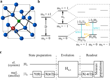
Figure 1: Constructing of $\mathcal{PT}$ symmetric Hamiltonian in NV center. a, Schematic atomic structure and energy levels of the NV center. b, Hyperfine structure of the coupling system with NV electron spin and ¹⁴N nuclear spin. The experiments are implemented on the two-qubit system composed of four energy levels $|m_{S}=0,m_{I}=+1\rangle$, $|m_{S}=-1,m_{I}=+1\rangle$, $|m_{S}=0,m_{I}=0\rangle$, and $|m_{S}=-1,m_{I}=0\rangle$ labeled by $|0\rangle_{e}|1\rangle_{n}$, $|0\rangle_{e}|0\rangle_{n}$, $|-1\rangle_{e}|1\rangle_{n}$, and $|-1\rangle_{e}|0\rangle_{n}$. The electronic zero-filed splitting is $D=2.87$ GHz and the Zeeman splitting of the electron spin is $\omega_{e}$. The two-qubit system is controlled by two microwave (MW) pulses (blue arrows) and two radio-frequency (RF) pulses (orange arrows), which selectively drive the two electron-spin transitions and the two nuclear-spin transitions, respectively. c, Quantum circuit of the experiment. The electron spin qubit is taken as the system qubit while the nuclear spin qubit is served as the ancilla qubit. X and Y denote the single nuclear spin qubit rotation around the x and y axes. The two-qubit system is prepared to $|\Psi(0)\rangle=|0\rangle_{e}|-\rangle_{n}+\eta_{0}(0)|0\rangle_{e}|+\rangle_{n}$ by rotations $\mathrm{Y}(\theta)$ and $\mathrm{X}(\pi/2)$. Then the two-qubit system evolve under the dilation Hamiltonian $H_{s,a}(t)$. The populations of the four energy levels are measured after the rotation $\mathrm{X}(-\pi/2)$.

The state evolution under the $\mathcal{PT}$ symmetric Hamiltonian $H_{s}$ is explored by monitoring $P_{0}$, i.e., the renormalized population of the state $|m_{S}=0\rangle$ of the electron spin when the nuclear spin state is in the selected state $|m_{I}=+1\rangle$ (see supplementary materials for details). The time of the state evolution is varied from 0 to 8 $\mathrm{\mu s}$. Figure 2a-d show the state evolution under $\mathcal{PT}$ symmetric Hamiltonian with the Hermitian case $r=0$ ( Fig. 2a ), $\mathcal{PT}$ unbroken case $r=0.6$ ( Fig. 2b ), exceptional point case $r=1.0$ ( Fig. 2c ) and $\mathcal{PT}$ broken case $r=1.4$ ( Fig. 2d ). All errors are one standard deviation with repeating the experiments for 0.5 million times. In the $\mathcal{PT}$ unbroken region, the time evolution of the state is periodic oscillation, while the oscillation breaks down in the $\mathcal{PT}$ broken region. The state evolutions under $\mathcal{PT}$ symmetric Hamiltonian with various values of the parameter, $r$, are shown in Fig. 2e-f. The $\mathcal{PT}$ phase transition threshold is evidently revealed at the exceptional point $r=1.0$. The experimental results (Fig. 2f) show good agreement with the corresponding theoretical predictions (Fig. 2e).

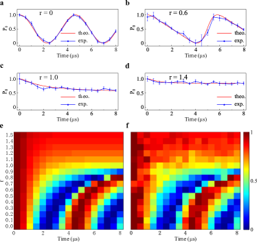
Figure 2: State evolution under $\mathcal{PT}$ symmetric Hamiltonian. a-d, Experimental state evolution under $\mathcal{PT}$ symmetric Hamiltonians with different parameter a of the Hamiltonian, where $r=0$ (a), $r=0.6$ (b), $r=1.0$ (c) and $r=1.4$ (d) correspond to the Hermitian, $\mathcal{PT}$ unbroken, exceptional point and $\mathcal{PT}$ broken case, respectively. $P_{0}$ is the renormalized population of the state $|m_{S}=0\rangle$ of the electron spin when the nuclear spin state is in the selected state $|m_{I}=+1\rangle$. Blue dots are experimental results, and red lines are the theoretical predictions. e (theoretical results ) and f (experimental results) plot results for various $r$ values. The color bar stands for the population $P_{0}$.

The $\mathcal{PT}$ phase transition is also characterized by the eigenvalues of the $\mathcal{PT}$ symmetric Hamiltonians as shown in Fig. 3. The eigenvalues of the $H_{s}$ can be achieved by $E_{\pm}=\pm\sqrt{1-r_{\mathrm{exp}}^{2}}$. The parameter $r_{\mathrm{exp}}$ is obtained by curve fitting the experimental time evolution of the population $P_{0}$ to theoretical predictions under $\mathcal{PT}$ symmetric Hamiltonian $H_{s}$ (see supplementary materials for the details). When $r<1$, the system is in a $\mathcal{PT}$ symmetry unbroken region. The eigenvalues $E$ are still real as $r$ approaches 1 from 0. At the exceptional point $r=1$, the eigenvalues $E$ coalesce to 0. The system is in the $\mathcal{PT}$ symmetry broken region when $r>1$. The real parts of the eigenvalues $E$ coalesce and the imaginary parts appears. The experimental results show excellent agreement with the corresponding theoretical predictions.

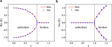
Figure 3: Experimental observation the breaking of the $\mathcal{PT}$ symmetry. a Real part and b imaginary part of the eigenvalues of the $\mathcal{PT}$ symmetric Hamiltonian. The blue dots are experimental data, and the red lines are the theoretical predictions of the eigenvalues. The $0<r<1$ regime represents the $\mathcal{PT}$ unbroken case and the $r>1$ regime represents the $\mathcal{PT}$ broken case. The exceptional point occurs at $r=1$.

In summary, we have experimentally demonstrate the state evolution under $\mathcal{PT}$ symmetric Hamiltonian by the Hermitian dilation method. The breaking of $\mathcal{PT}$ symmetry has been observed in a single electron spin. The universal dilation method present here is compatible for Hermitian dilation of an arbitrary non-Hermitian Hamiltonian, thus our work opens a door for future experimental study of the intriguing non-Hermitian and $\mathcal{PT}$ symmetric physics with quantum systems.

This work was supported by the National Key R$\&$D Program of China (Grants No. 2018YFA0306600 and No. 2016YFB0501603), the CAS (Grants No. GJJSTD20170001, No.QYZDY-SSW-SLH004 and No.QYZDB-SSW-SLH005), and Anhui Initiative in Quantum Information Technologies (Grant No. AHY050000). X.R. thanks the Youth Innovation Promotion Association of Chinese Academy of Sciences for the support.

APPENDIX

I I. Universal Hermitian dilation of non-Hermitian Hamiltonians

This section mainly focus on universally dilating a non-Hermitian Hamiltonian into a Hermitian one. Subsection A demonstrates the dilation method, followed by some derivation used in the dilation in subsection B and subsection C. Finally, in subsection D the universality of this method is proved.

I.1 A. Universal dilation method

Our target is to realize the dynamics of a quantum system $s$, which is described by the evolution $\varepsilon_{1}(t)$ governed by Hamiltonian $H_{s}(t)$. $H_{s}(t)$ is non-Hermitian, arbitrary dimensional and time-dependent in general. The state evolution of system $s$ is described by $|\psi(t)\rangle$, so the corresponding Schrödinger equation can be written as (natural unit are chosen so that $\hbar=1$ in this supplementary material)

$$i\frac{d}{dt}|\psi(t)\rangle=H_{s}(t)|\psi(t)\rangle.$$ (S1)

To realize $\varepsilon_{1}(t)$ in a quantum system, an ancilla qubit is introduced to dilate $H_{s}(t)$ into a Hermitian Hamiltonian $H_{s,a}(t)$. The evolution of the combined system under $H_{s,a}(t)$ is $\varepsilon_{2}(t)$. The state evolution of the combined system is described by $|\Psi(t)\rangle$, which satisfies the following Schrödinger equation

$$i\frac{d}{dt}|\Psi(t)\rangle=H_{s,a}(t)|\Psi(t)\rangle.$$ (S2)

$|\Psi(t)\rangle$ is a dilation of $|\psi(t)\rangle$ and can be written as

$$\left\{\begin{aligned} &|\Psi(t)\rangle=|\psi(t)\rangle|-\rangle+|\chi(t)\rangle|+\rangle,\\ &|\chi(t)\rangle=\eta(t)|\psi(t)\rangle,\\ \end{aligned}\right.$$ (S3)

where $|-\rangle=\frac{|0\rangle-i|1\rangle}{\sqrt{2}}$ and $|+\rangle=-i\frac{|0\rangle+i|1\rangle}{\sqrt{2}}$ are the eigenstates of Pauli operator $\sigma_{y}$, which forms an orthonormal basis of the ancilla qubit, and $\eta(t)$ is a linear operator. When a measurement is applied on the ancilla qubit and $|-\rangle$ is postselected, the evolution $\varepsilon_{1}(t)$ governed by the non-Hermitian Hamiltonian $H_{s}(t)$ can be produced.

Now the key is to derive the expression of $H_{s,a}(t)$. The mathematical form of $H_{s,a}(t)$ can be written as

$$H_{s,a}(t)=H_{s,a}^{(++)}(t)\otimes|+\rangle\langle+|+H_{s,a}^{(+-)}(t)\otimes|+\rangle\langle-|+H_{s,a}^{(-+)}(t)\otimes|-\rangle\langle+|+H_{s,a}^{(--)}(t)\otimes|-\rangle\langle-|,$$ (S4)

where $H_{s,a}^{(++)}(t),H_{s,a}^{(+-)}(t),H_{s,a}^{(-+)}(t)$ and $H_{s,a}^{(--)}(t)$ have the same dimension as $H_{s}(t)$. Due to the Hermiticity of $H_{s,a}(t)$, we have

$$\left\{\begin{aligned} &H_{s,a}^{(++)\dagger}(t)=H_{s,a}^{(++)}(t),\\ &H_{s,a}^{(+-)\dagger}(t)=H_{s,a}^{(-+)}(t),\\ &H_{s,a}^{(--)\dagger}(t)=H_{s,a}^{(--)}(t).\\ \end{aligned}\right.$$ (S5)

By substituting equations S1, S3 and S4 into equation S2 and rearranging terms, we obtain

$$\left\{\begin{aligned} &H_{s,a}^{(--)}(t)+H_{s,a}^{(-+)}(t)\eta(t)-H_{s}(t)=0,\\ &H_{s,a}^{(+-)}(t)+H_{s,a}^{(++)}(t)\eta(t)-i\frac{d}{dt}\eta(t)-\eta(t)H_{s}(t)=0.\\ \end{aligned}\right.$$ (S6)

After taking Hermitian transpose of operators in equation S6 we can get

$$\left\{\begin{aligned} &H_{s,a}^{(--)}(t)+\eta^{\dagger}(t)H_{s,a}^{(+-)}(t)-H_{s}^{\dagger}(t)=0,\\ &H_{s,a}^{(-+)}(t)+\eta^{\dagger}(t)H_{s,a}^{(++)}(t)+i\frac{d}{dt}\eta^{\dagger}(t)-H_{s}^{\dagger}(t)\eta^{\dagger}(t)=0,\\ \end{aligned}\right.$$ (S7)

where equation S5 has been taken into consideration. Finally, equations S6 and S7 reduce to

$$\left\{\begin{aligned} &H_{s,a}^{(--)}(t)=H_{s}(t)-[H_{s}^{\dagger}(t)\eta^{\dagger}(t)-i\frac{d}{dt}\eta^{\dagger}(t)-\eta^{\dagger}(t)H_{s,a}^{(++)}(t)]\eta(t),\\ &H_{s,a}^{(-+)}(t)=H_{s}^{\dagger}(t)\eta^{\dagger}(t)-i\frac{d}{dt}\eta^{\dagger}(t)-\eta^{\dagger}(t)H_{s,a}^{(++)}(t),\\ &H_{s,a}^{(+-)}(t)=\eta(t)H_{s}(t)+i\frac{d}{dt}\eta(t)-H_{s,a}^{(++)}(t)\eta(t),\\ \end{aligned}\right.$$ (S8)

together with an equation that $\eta(t)$ should satisfy,

$$i\frac{d}{dt}[\eta^{\dagger}(t)\eta(t)]=H_{s}^{\dagger}(t)[\eta^{\dagger}(t)\eta(t)+I]-[\eta^{\dagger}(t)\eta(t)+I]H_{s}(t).$$ (S9)

To solve equation S9 , we can define a Hermitian operator $M(t)$ as follows

$$M(t)\equiv\eta^{\dagger}(t)\eta(t)+I,$$ (S10)

where $I$ is the identity operator. Then equation S9 can be rewritten as

$$i\frac{d}{dt}M(t)=H_{s}^{\dagger}(t)M(t)-M(t)H_{s}(t).$$ (S11)

The solution of equation S11 takes the form

$$M(t)=\mathcal{T}e^{-i\int_{0}^{t}H_{s}^{\dagger}(t)dt}M(0)\overline{\mathcal{T}}e^{i\int_{0}^{t}H_{s}(t)dt},$$ (S12)

where $\mathcal{T}$ and $\overline{\mathcal{T}}$ are time-ordering and anti-time-ordering operators, respectively. $M(0)$ is an initial operator of operator $M(t)$, which is chosen to ensure that $M(t)-I$ keeps positive for all $t$. According to equation S10, an expression of $\eta(t)$ can be written as

$$\eta(t)=U(t)[M(t)-I]^{\frac{1}{2}},$$ (S13)

where $U(t)$ is an arbitrary differentiable unitary operator. Equation S4, S8, S12 together with equation S13 give an explicit expression of the dilated Hamiltonian $H_{s,a}(t)$, in which $H_{s,a}^{(++)}(t)$ is an arbitrary Hamiltonian operator.

Note that $H_{s,a}(t)$ is not uniquely determined since $H_{s,a}^{(++)}(t)$ can be an arbitrary Hermitian operator and $U(t)$ can be an arbitrary differentiable unitary operator. This arbitrariness makes it possible to flexible design $H_{s,a}(t)$ according to different experimental systems. For example, to make $H_{s,a}(t)$ easy to be constructed in NV center, we can choose

$$\left\{\begin{aligned} &U(t)=I,\\ &H_{s,a}^{(++)}(t)=\{H_{s}(t)+[i\frac{d}{dt}\eta(t)+\eta(t)H_{s}(t)]\eta(t)\}M^{-1}(t).\end{aligned}\right.$$ (S14)

The Hermiticity of $H_{a,s}^{(++)}(t)$ will be proved in subsection B of this section. According to equation S14, equation S13 reduces to

$$\eta(t)=[M(t)-I]^{\frac{1}{2}},$$ (S15)

which means $\eta(t)$ is also a Hermitian operator. In this case the Hermitian operator,

$$M(t)=\eta^{\dagger}(t)\eta(t)+I=\eta^{2}(t)+I,$$ (S16)

commutes with $\eta(t)$, and the inverse operator of $M(t)$, $M^{-1}(t)$, is Hermitian and commutes with $\eta(t)$ as well. By substituting equation S14 into equation S8 and considering the Hermiticity of $\eta(t)$, we have

$$\left\{\begin{aligned} &H_{s,a}^{(--)}(t)=H_{s}(t)-H_{s}^{\dagger}(t)\eta^{2}(t)+i[\frac{d}{dt}\eta(t)]\eta(t)+\eta(t)\{H_{s}(t)+[i\frac{d}{dt}\eta(t)+\eta(t)H_{s}(t)]\eta(t)\}M^{-1}(t)\eta(t),\\ &H_{s,a}^{(-+)}(t)=H_{s}^{\dagger}(t)\eta(t)-i\frac{d}{dt}\eta(t)-\eta(t)\{H_{s}(t)+[i\frac{d}{dt}\eta(t)+\eta(t)H_{s}(t)]\eta(t)\}M^{-1}(t),\\ &H_{s,a}^{(+-)}(t)=\eta(t)H_{s}(t)+i\frac{d}{dt}\eta(t)-\{H_{s}(t)+[i\frac{d}{dt}\eta(t)+\eta(t)H_{s}(t)]\eta(t)\}M^{-1}(t)\eta(t).\\ \end{aligned}\right.$$ (S17)

Equation S17 can be simplified to

$$\left\{\begin{aligned} &H_{s,a}^{(--)}(t)=\{H_{s}(t)+[i\frac{d}{dt}\eta(t)+\eta(t)H_{s}(t)]\eta(t)\}M^{-1}(t),\\ &H_{s,a}^{(-+)}(t)=[H_{s}(t)\eta(t)-\eta(t)H_{s}(t)-i\frac{d}{dt}\eta(t)]M^{-1}(t),\\ &H_{s,a}^{(+-)}(t)=-[H_{s}(t)\eta(t)-\eta(t)H_{s}(t)-i\frac{d}{dt}\eta(t)]M^{-1}(t).\\ \end{aligned}\right.$$ (S18)

The detail of the derivation from equation S17 to equation S18 is given in subsection C of this section. Substituting equation S18 and equation S14 into equation S4, we obtain

$$H_{s,a}(t)= \{\{H_{s}(t)+[i\frac{d}{dt}\eta(t)+\eta(t)H_{s}(t)]\eta(t)\}\otimes|+\rangle\langle+|-[H_{s}(t)\eta(t)-\eta(t)H_{s}(t)-i\frac{d}{dt}\eta(t)]\otimes|+\rangle\langle-|$$ (S19)

$$+[H_{s}(t)\eta(t)-\eta(t)H_{s}(t)-i\frac{d}{dt}\eta(t)]\otimes|-\rangle\langle+|+\{H_{s}(t)+[i\frac{d}{dt}\eta(t)+\eta(t)H_{s}(t)]\eta(t)\}\otimes|-\rangle\langle-|\}M^{-1}(t),$$

or

$$H_{s,a}(t)=\Lambda(t)\otimes I+\Gamma(t)\otimes\sigma_{z},$$ (S20)

with

$$\left\{\begin{aligned} &\Lambda(t)=\{H_{s}(t)+[i\frac{d}{dt}\eta(t)+\eta(t)H_{s}(t)]\eta(t)\}M^{-1}(t),\\ &\Gamma(t)=i[H_{s}(t)\eta(t)-\eta(t)H_{s}(t)-i\frac{d}{dt}\eta(t)]M^{-1}(t).\\ \end{aligned}\right.$$ (S21)

I.2 B. Proof of the Hermiticity of $H_{s,a}^{(++)}(t)$

Utilizing the commutation relation between $M(t)$ and $\eta(t)$, the second formula of equation S14 can be rewritten as

$$H_{s,a}^{(++)}(t)=M^{-1}(t)\{M(t)H_{s}(t)+\eta(t)M(t)H_{s}(t)\eta(t)+iM(t)[\frac{d}{dt}\eta(t)]\eta(t)\}M^{-1}(t).$$ (S22)

By substituting equation S16 into the third term of the right-hand side of equation S22, we obtain

$$H_{s,a}^{++}(t)=M^{-1}(t)\{M(t)H_{s}(t)+\eta(t)M(t)H_{s}(t)\eta(t)+i\eta^{2}(t)[\frac{d}{dt}\eta(t)]\eta(t)+i[\frac{d}{dt}\eta(t)]\eta(t)\}M^{-1}(t).$$ (S23)

Considering the Hermiticity of $\eta(t)$, $M(t)$ and $M^{-1}(t)$, the Hermitian conjunction operator of $H_{a,s}^{(++)}(t)$ can be written as

$$H_{s,a}^{(++){\dagger}}(t)=M^{-1}(t)\{H_{s}^{\dagger}(t)M(t)+\eta(t)H_{s}^{\dagger}(t)M(t)\eta(t)-i\eta(t)[\frac{d}{dt}\eta(t)]\eta^{2}(t)-i\eta(t)[\frac{d}{dt}\eta(t)]\}M^{-1}(t).$$ (S24)

Combining equation S23 and equation S24, we have

$$H_{s,a}^{(++){\dagger}}(t)-H_{s,a}^{++}(t)$$ (S25)

$$= M^{-1}(t)[H_{s}^{\dagger}(t)M(t)-M(t)H_{s}(t)]M^{-1}(t)+M^{-1}(t)\eta(t)[H_{s}^{\dagger}(t)M(t)-M(t)H_{s}(t)]\eta(t)M^{-1}(t)$$

$$-iM^{-1}(t)\eta(t)\{[\frac{d}{dt}\eta(t)]\eta(t)+\eta(t)[\frac{d}{dt}\eta(t)]\}\eta(t)M^{-1}(t)-iM^{-1}(t)\{\eta(t)[\frac{d}{dt}\eta(t)]+\frac{d}{dt}\eta(t)]\eta(t)\}M^{-1}(t).$$

According to equation S11 and equation S16, we have

$$i\frac{d}{dt}M(t)=H_{s}^{\dagger}(t)M(t)-M(t)H_{s}(t)=i\{[\frac{d}{dt}\eta(t)]\eta(t)+\eta(t)[\frac{d}{dt}\eta(t)]\}.$$ (S26)

Then, equation S25 vanishes, so the Hermiticity of $H_{s,a}^{(++)}(t)$ is proved.

I.3 C. Derivation of the form of $H_{s,a}^{(--)}(t),H_{s,a}^{(-+)}(t)$ and $H_{s,a}^{(+-)}(t)$

The first formula in equation S17 reads

$$H_{s,a}^{(--)}(t)=H_{s}(t)-H_{s}^{\dagger}(t)\eta^{2}(t)+i[\frac{d}{dt}\eta(t)]\eta(t)+\eta(t)\{H_{s}(t)+[i\frac{d}{dt}\eta(t)+\eta(t)H_{s}(t)]\eta(t)\}M^{-1}(t)\eta(t).$$ (S27)

Substitute equation S16 into equation S27 and consider the commutation of $M^{-1}(t)$ and $\eta(t)$ we have

$$H_{s,a}^{(--)}(t)= -H_{s}^{\dagger}(t)M(t)+H_{s}^{\dagger}(t)+i[\frac{d}{dt}\eta(t)]\eta(t)+\eta(t)H_{s}(t)\eta(t)M^{-1}(t)$$ (S28)

$$+i\eta(t)[\frac{d}{dt}\eta(t)][M(t)-I]M^{-1}(t)+[M(t)-I]H_{s}(t)[M(t)-I]M^{-1}(t)+H_{s}(t).$$

Simplify and rearrange terms in equation S28, we obtain

$$H_{s,a}^{(--)}(t)= -[H_{s}^{\dagger}(t)M(t)-M(t)H_{s}(t)]+i\{[\frac{d}{dt}\eta(t)]\eta(t)+\eta(t)[\frac{d}{dt}\eta(t)]\}$$ (S29)

$$+\{H_{s}(t)+\eta(t)H_{s}(t)\eta(t)-i\eta(t)[\frac{d}{dt}\eta(t)]+[H_{s}^{\dagger}(t)M(t)-M(t)H_{s}(t)]\}M^{-1}(t),$$

then, by substituting equations S26 into equation S29 and rearranging terms, equation S29 reduces to

$$H_{s,a}^{(--)}(t)=\{H_{s}(t)+[i\frac{d}{dt}\eta(t)+\eta(t)H_{s}(t)]\eta(t)\}M^{-1}(t),$$ (S30)

which is the first formula in equation S18.

The third formula in equation S17 is given by

$$H_{s,a}^{(+-)}(t)=\eta(t)H_{s}(t)+i\frac{d}{dt}\eta(t)-\{H_{s}(t)+[i\frac{d}{dt}\eta(t)+\eta(t)H_{s}(t)]\eta(t)\}M^{-1}(t)\eta(t).$$ (S31)

Considering the commutation of $M^{-1}(t)$ and $\eta(t)$, and substituting equation S16, we have

$$H_{s,a}^{(+-)}(t)=\eta(t)H_{s}(t)+i\frac{d}{dt}\eta(t)-H_{s}(t)\eta(t)M^{-1}(t)-[i\frac{d}{dt}\eta(t)+\eta(t)H_{s}(t)][M(t)-I]M^{-1}(t).$$ (S32)

Equation S32 reduces to

$$H_{s,a}^{(+-)}(t)=-[H_{s}(t)\eta(t)-\eta(t)H_{s}(t)-i\frac{d}{dt}\eta(t)]M^{-1}(t),$$ (S33)

so the third formula in equation S18 is proved.

To prove the second formula in equation S18, we rewrite equation S33 as

$$H_{s,a}^{(+-)}(t)=-M^{-1}(t)[M(t)H_{s}(t)\eta(t)-\eta(t)M(t)H_{s}(t)-i\eta^{2}(t)\frac{d}{dt}\eta(t)-i\frac{d}{dt}\eta(t)]M^{-1}(t),$$ (S34)

where equation S16 and commutation of $M(t)$ and $\eta(t)$ have been utilized. According to equation S5, $H_{s,a}^{(-+)}(t)=H_{s,a}^{(+-){\dagger}}(t)$, we have

$$H_{s,a}^{(-+)}(t)=-M^{-1}(t)\{\eta(t)H_{s}^{\dagger}(t)M(t)-H_{s}^{\dagger}(t)M(t)\eta(t)+i[\frac{d}{dt}\eta(t)]\eta^{2}(t)+i\frac{d}{dt}\eta(t)\}M^{-1}(t),$$ (S35)

where the Hermiticity of $\eta(t)$, $M(t)$ and $M^{-1}(t)$ have been considered. Combining equation S34 and equation S35, we obtain

$$H_{s,a}^{(-+)}(t)+H_{s,a}^{(+-)}(t)= -M^{-1}(t)\{\eta(t)[H_{s}^{\dagger}(t)M(t)-M(t)H_{s}(t)]-$$ (S36)

$$[H_{s}^{\dagger}(t)M(t)-M(t)H_{s}(t)]\eta(t)+i[\frac{d}{dt}\eta(t)]\eta^{2}(t)-i\eta^{2}(t)\frac{d}{dt}\eta(t)\}M^{-1}(t).$$

Substituting equation S26 into equation S36, we have

$$H_{s,a}^{(-+)}(t)+H_{s,a}^{(+-)}(t)= -M^{-1}(t)\{i\eta(t)[\frac{d}{dt}\eta(t)]\eta(t)+i\eta^{2}(t)[\frac{d}{dt}\eta(t)]-i[\frac{d}{dt}\eta(t)]\eta^{2}(t)-i\eta(t)[\frac{d}{dt}\eta(t)]\eta(t)$$ (S37)

$$+i[\frac{d}{dt}\eta(t)]\eta^{2}(t)-i\eta^{2}(t)\frac{d}{dt}\eta(t)\}M^{-1}(t).$$

By canceling terms, equation S37 vanishes, that is

$$H_{s,a}^{(-+)}(t)=-H_{s,a}^{(+-)}(t)=[H_{s}(t)\eta(t)-\eta(t)H_{s}(t)-i\frac{d}{dt}\eta(t)]M^{-1}(t),$$ (S38)

which is the second formula in equation S18.

I.4 D. Proof of the universality of this dilation method

Here we show that our method can be utilized for Hermitian dilation of an arbitraty Hamiltonian $H_{s}(t)$. Without loss of generality, the evolution time is denoted by $T$, so $t\in[0,T]$ during the evolution. Since $H_{s}(t)$ is a Hamiltonian governing the evolution of a quantum system, given the state $|\psi(t_{1})\rangle=|\psi_{1}\rangle$ at any time point $t_{1}\in[0,T]$, the subsequent state evolution is uniquely determined by $H_{s}(t)$. That is, the Schrödinger equation with an initial value,

$$\left\{\begin{aligned} &i\frac{d}{dt}|\psi(t)\rangle=H_{s}(t)|\psi(t)\rangle,\\ &|\psi(t_{1})\rangle=|\psi_{1}\rangle,\end{aligned}\right.$$ (S39)

has a unique solution on $[t_{1},T]$. Stated another way, the evolution operator

$$\varepsilon_{1}(t;t_{1})=\mathcal{T}e^{-i\int_{t_{1}}^{t}H_{s}(t)dt},$$ (S40)

exist on $[t_{1},T]$. Obviously, $\varepsilon_{1}(t_{1};t_{1})=I$ for any $t_{1}\in[0,T]$.

It can be proved that $\varepsilon_{1}(t;t_{1})$ is an invertible operator for $t\in[0,T]$ as follows. Suppose that $\varepsilon_{1}(t;t_{1})$ is not invertible, then we can divide the evolution time into several segments, for example, $[t_{1},t]=[t_{1},t_{2}]\cup[t_{2},t_{3}]\cup...\cup[t_{k-1},t_{k}]\cup[t_{k},t]$, where $t_{1}<t_{2}<t_{3}<...<t_{k}<t$, in this case, we have

$$\varepsilon_{1}(t;t_{1})=\varepsilon_{1}(t;t_{k})\varepsilon_{1}(t_{k};t_{k-1})...\varepsilon_{1}(t_{3};t_{2})\varepsilon_{1}(t_{2};t_{1}).$$ (S41)

If $\varepsilon_{1}(t;t_{1})$ is not invertible, there must be at least a segment corresponding to which the evolution operator is not invertible. Without loss of generality, suppose $\varepsilon_{1}(t_{n+1};t_{n})$, the evolution operator on $[t_{n},t_{n+1}]$ where $t_{1}<t_{n}<t_{n+1}<t$, is not invertible. The segment $[t_{n},t_{n+1}]$ can be further divided into several subsegments. Similarity, there is at least a subsegment corresponding to which the evolution operator is not invertible. The division can be implemented for arbitrary times. As a result, there is a segment with infinitesimal length and the corresponding evolution operator is not invertible. However, an evolution operator with infinitesimal time duration tends to $I$, which is invertible. The contradiction shows that $\varepsilon_{1}(t;t_{1})$ must be an invertible operator,then the inverse operator of $\varepsilon_{1}(t;t_{1})$ can be written as

$$\varepsilon_{1}^{-1}(t;t_{1})=\overline{\mathcal{T}}e^{i\int_{t_{1}}^{t}H_{s}(t)dt}.$$ (S42)

According to the derivation of $H_{s,a}(t)$ in part one, the dilated Hamiltonian $H_{s,a}(t)$ can be obtained once a differentiable $\eta(t)$, which is a solution of equation S9, is derived. Equations S12 and S13 provide the solution to equation S9, given that $M(t)$ is a positive operator with all eigenvalues larger than $1$ during the evolution. It will be shown in the following that, by appropriate selection of the initial operator $M(0)$, the aforementioned requirement can be always satisfied for an arbitrary Hamiltonian $H_{s}(t)$. To start with, select a positive operator $M_{0}^{\prime}$, of which all the eigenvalues are larger than $1$. Then $M(0)^{\prime}$ is invertible and can be expressed as

$$M_{0}^{\prime}=\zeta^{\dagger}\zeta.$$ (S43)

Define

$$M^{\prime}(t)\equiv\mathcal{T}e^{-i\int_{0}^{t}H_{s}^{\dagger}(t)dt}M(0)^{\prime}\overline{\mathcal{T}}e^{i\int_{0}^{t}H_{s}(t)dt}$$ (S44)

then

$$M^{\prime}(t)=(\zeta\overline{\mathcal{T}}e^{i\int_{0}^{t}H_{s}(t)dt})^{\dagger}(\zeta\overline{\mathcal{T}}e^{i\int_{0}^{t}H_{s}(t)dt}),$$ (S45)

is a positive operator. Because $\overline{\mathcal{T}}e^{i\int_{0}^{t}H_{s}(t)dt}=\varepsilon_{1}^{-1}(t;0)$, $M_{0}^{\prime}$, and $\mathcal{T}e^{-i\int_{0}^{t}H_{s}^{\dagger}(t)dt}=[\varepsilon_{1}^{-1}(t;0)]^{\dagger}$ are all invertible operators, then according to equation S45, $M^{\prime}(t)$ is an invertible operator. Therefore, all the eigenvalues of $M^{\prime}(t)$ are larger than $0$. Suppose the minimum of the eigenvalues of $M^{\prime}(t)$ is $\mu^{\prime}$, then $\mu^{\prime}>0$. Take $0<\mu<\mu^{\prime}$ and $M(0)=M_{0}^{\prime}/\mu$, then

$$M(t)=\frac{1}{\mu}M^{\prime}(t),$$ (S46)

is a positive operator with all eigenvalues larger than $1$ during the evolution. Therefore, the dilated Hamiltonian $H_{s,a}(t)$ can be obtained with our method for an arbitrary Hamiltonian $H_{s}(t)$.

II II. Construct Hamiltonian $H_{s,a}(t)$ in NV center

The dilated Hamiltonian shown in equation S20 takes the form

$$H_{s,a}(t)=\Lambda(t)\otimes I+\Gamma(t)\otimes\sigma_{z},$$ (S47)

where operators $\Lambda(t)$ and $\Gamma(t)$ are given in equation S21. By expanding $\Lambda(t)$ and $\Gamma(t)$ in terms of Pauli operators, we can rewrite $H_{s,a}(t)$ as

$$H_{s,a}(t)= B_{1}(t)I\otimes I+A_{1}(t)\sigma_{x}\otimes I+B_{2}(t)\sigma_{y}\otimes I+B_{3}(t)\sigma_{z}\otimes I+$$ (S48)

$$A_{2}(t)I\otimes\sigma_{z}+B_{4}(t)\sigma_{x}\otimes\sigma_{z}+A_{3}(t)\sigma_{y}\otimes\sigma_{z}+A_{4}(t)\sigma_{z}\otimes\sigma_{z},$$

where $A_{i}(t)$ and $B_{i}(t)$, $i\in[1,4]$, are the corresponding decomposition coefficients (real parameters). According to our numerical calculation, coefficients $B_{i}(t),i\in[1,4],$ vanish because of the form of the $H_{s}$ we choose. In this case, $H_{s,a}(t)$ reduces to

$$H_{s,a}(t)=A_{1}(t)\sigma_{x}\otimes I+A_{2}(t)I\otimes\sigma_{z}+A_{3}(t)\sigma_{y}\otimes\sigma_{z}+A_{4}(t)\sigma_{z}\otimes\sigma_{z}.$$ (S49)

Fig. S1 shows the parameters $A_{i}(t)$ ($i=1,2,3,4$) of the corresponding dilated Hamiltonian $H_{s,a}(t)$ when $H_{s}$ is in the region of unbroken $PT$ symmetry (Fig. S1.(a)), at the exceptional point (Fig. S1.(b)), and in the region of broken $PT$ symmetry (Fig. S1.(c)), respectively.

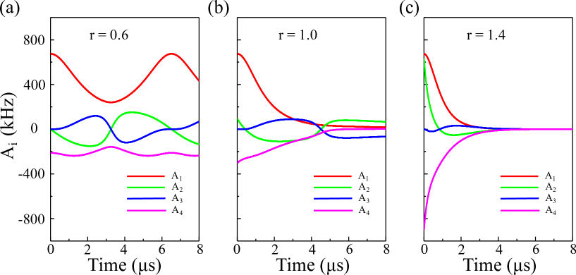
Figure S1: Parameters $A_{i}(t)$ in the dilated Hamiltonian. Parameters $A_{i}(t)$ ($i=1,2,3,4$) in the dilated Hamiltonian $H_{s,a}(t)$ as a function of t for (a) $r=0.6$, (b) $r=1.0$ and (c) $r=1.4$.

NV center is a kind of point defect in diamond consisting of a substitutional nitrogen atom and an adjoint vacancy. The electron spin and nuclear spin in NV center consist a highly controllable two-qubit solid-state system. The electron spin with a spin triple ground state ($S=1$) is coupled with the nearby ${}^{14}\mathrm{N}$ nuclear spin. By applying an external magnetic field $B_{0}$ along the NV axis, the Hamiltonian of NV center can be written as

$$H_{\mathrm{NV}}=2\pi(DS_{z}^{2}+\omega_{e}S_{z}+QI_{z}^{2}+\omega_{n}I_{z}+AS_{z}I_{z}),$$ (S50)

where $\omega_{e}=-\gamma_{e}B_{0}/2\pi$ ($\omega_{n}=-\gamma_{n}B_{0}/2\pi$) is the Zeeman splitting of the electron (${}^{14}\mathrm{N}$ nuclear) spin, with $\gamma_{e}$ ($\gamma_{n}$) being the electron (${}^{14}\mathrm{N}$ nuclear) gyromagnetic ratio. $S_{z}$ and $I_{z}$ are the spin operators of the electron spin (spin-1) and the ${}^{14}\mathrm{N}$ nuclear spin (spin-1), respectively. $D=2.87$ GHz is the axial zero-field splitting parameter for the electron spin. $Q=-4.95$ MHz is the quadrupole splitting parameter of the ${}^{14}\mathrm{N}$ nuclear spin. $A=-2.16$ MHz is the hyperfine coupling parameter.

The experiment is performed in the two qubit subspace spanned by $|m_{s}=0,m_{I}=1\rangle,|m_{s}=0,m_{I}=0\rangle,|m_{s}=-1,m_{I}=1\rangle,$ and $|m_{s}=-1,m_{I}=0\rangle$, labeled by $|0\rangle_{e}|1\rangle_{n},|0\rangle_{e}|0\rangle_{n},|-1\rangle_{e}|1\rangle_{n}$ and $|-1\rangle_{e}|0\rangle_{n}$, in which the Hamiltonian can be simplified as

$$H_{0}=\pi[-(D-\omega_{e}-\frac{A}{2})\sigma_{z}\otimes I+(Q+\omega_{n}-\frac{A}{2})I\otimes\sigma_{z}+\frac{A}{2}\sigma_{z}\otimes\sigma_{z}].$$ (S51)

To construct $H_{s,a}(t)$ in NV center, we can apply two slightly detuned microwave (MW) pulses to selectively drive the two electron spin transitions, as depicted in Fig. 1b in the main text. The total Hamiltonian in the two qubit subspace when applying MW pulses can be written as

$$H_{\mathrm{tot}}= \pi[-(D-\omega_{e}-\frac{A}{2})\sigma_{z}\otimes I+(Q+\omega_{n}-\frac{A}{2})I\otimes\sigma_{z}+\frac{A}{2}\sigma_{z}\otimes\sigma_{z}]$$ (S52)

$$+2\pi\Omega_{1}(t)\cos[\int_{0}^{t}\omega_{1}(\tau)d\tau+\phi_{1}(t)]\sigma_{x}\otimes|1\rangle_{n}~{}_{n}\langle 1|+2\pi\Omega_{2}(t)\cos[\int_{0}^{t}\omega_{2}(\tau)d\tau+\phi_{2}(t)]\sigma_{x}\otimes|0\rangle_{n}~{}_{n}\langle 0|,$$

where $\Omega_{1}(t)$, $\omega_{1}(t)$ and $\phi_{1}(t)$ ($\Omega_{2}(t)$, $\omega_{2}(t)$ and $\phi_{2}(t)$) are the Rabi frequency, angular frequency and phase of the MW pulses which drive the electron spin transition if the nuclear spin is $|1\rangle_{n}$ ($|0\rangle_{n}$). By choosing interaction picture

$$U_{rot}=e^{i\int_{0}^{t}[H_{0}-A_{2}(\tau)I\otimes\sigma_{z}-A_{4}(\tau)\sigma_{z}\otimes\sigma_{z}]d\tau},$$ (S53)

the total Hamiltonian transforms to

$$H_{rot}= U_{rot}H_{tot}U_{rot}^{\dagger}-iU_{rot}\frac{dU_{rot}^{\dagger}}{dt}$$ (S54)

$$= A_{2}(t)I\otimes\sigma_{z}+A_{4}(t)\sigma_{z}\otimes\sigma_{z}$$

$$+2\pi\Omega_{1}(t)\cos[\int_{0}^{t}\omega_{1}(\tau)d\tau+\phi_{1}(t)]\{\cos[\omega_{MW1}t+\int_{0}^{t}2A_{4}(\tau)d\tau]\sigma_{x}+\sin[\omega_{MW1}t+\int_{0}^{t}2A_{4}(\tau)d\tau]\sigma_{y}\}\otimes|1\rangle_{n}~{}_{n}\langle 1|$$

$$+2\pi\Omega_{2}(t)\cos[\int_{0}^{t}\omega_{2}(\tau)d\tau+\phi_{2}(t)]\{\cos[\omega_{MW2}t-\int_{0}^{t}2A_{4}(\tau)d\tau]\sigma_{x}+\sin[\omega_{MW2}t-\int_{0}^{t}2A_{4}(\tau)d\tau]\sigma_{y}\}\otimes|0\rangle_{n}~{}_{n}\langle 0|,$$

with $\omega_{MW1}$($\omega_{MW2}$) being the energy difference between $|0\rangle_{e}|1\rangle_{n}$ and $|-1\rangle_{e}|1\rangle_{n}$ ($|0\rangle_{e}|0\rangle_{n}$ and $|-1\rangle_{e}|0\rangle_{n}$). By choosing

$$\left\{\begin{aligned} &\omega_{1}(t)=\omega_{MW1}+2A_{4}(t)\\ &\omega_{2}(t)=\omega_{MW2}-2A_{4}(t)\\ &\Omega_{1}(t)=\Omega_{2}(t)=\Omega(t)\\ &-\phi_{1}(t)=\phi_{2}(t)=\phi(t)\end{aligned},\right.$$ (S55)

then in the condition of rotating wave approximation, $H_{rot}$ can be reduced to

$$H_{rot}=A_{2}(t)I\otimes\sigma_{z}+A_{4}(t)\sigma_{z}\otimes\sigma_{z}+\pi\Omega(t)\cos[\phi(t)]\sigma_{x}\otimes I+\pi\Omega(t)\sin[\phi(t)]\sigma_{y}\otimes I.$$ (S56)

Comparing equation S56 with equation S51, we can choose

$$\left\{\begin{aligned} &\Omega(t)=\frac{\sqrt{A_{1}^{2}(t)+A_{3}^{2}(t)}}{2\pi},\\ &\phi(t)=\arctan\frac{A_{3}(t)}{A_{1}(t)},\\ \end{aligned}\right.$$ (S57)

to realize Hamiltonian $H_{s,a}(t)$.

III III. Characterization of $\psi(t)$

The state of the system after the evolution governed by the dilated Hamiltonian $H_{s,a}(t)$ is

$$|\Psi(t)\rangle=|\psi(t)\rangle_{e}|-\rangle_{n}+\eta_{0}(t)|\psi(t)\rangle_{e}|+\rangle_{n}.$$ (S58)

By applying a rotation of $\pi/2$ along $\mathrm{-X}$ axis on the nuclear spin qubit, as depected in Fig. 1c in the main text, the state evolutes to

$$|\Phi(t)\rangle=|\psi(t)\rangle_{e}|1\rangle_{n}+\eta_{0}(t)|\psi(t)\rangle_{e}|0\rangle_{n}.$$ (S59)

Thus the evolution $|\psi(t)\rangle_{e}$ governed by $\mathcal{PT}$ symmetric Hamiltonian $H_{s}$ can be characterized by $P_{0}$, the normalized population of state $|0\rangle_{e}|1\rangle_{n}$ after selecting $|1\rangle_{n}$. $P_{0}$ can be calculated by $P_{0}=P_{|0\rangle_{e}|1\rangle_{n}}/(P_{|0\rangle_{e}|1\rangle_{n}}+P_{|-1\rangle_{e}|1\rangle_{n}})$, with $P_{|0\rangle_{e}|1\rangle_{n}}$ ($P_{|-1\rangle_{e}|1\rangle_{n}}$) being the population of state $|0\rangle_{e}|1\rangle_{n}$ ($|-1\rangle_{e}|1\rangle_{n}$) of state $|\Phi(t)\rangle$. This can be acquired by measuring the population distributon of the final state.

The four levels we choose to perform our experiment give rise to different photoluminescence(PL) rates[PRB_Steiner, ], providing information of the population distribution of the final state. However, different distributions can present the same PL rate, thus a set of pulse sequences are needed to determine the population distribution.

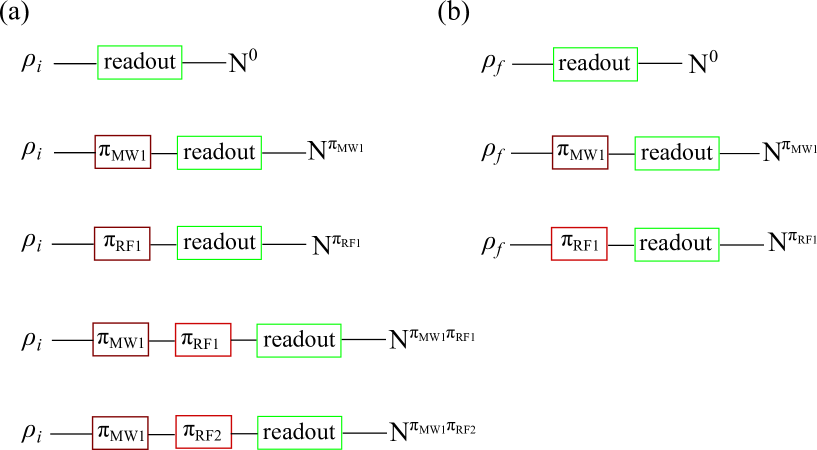
Figure S2: Schematic normalization and measurement sequences. Here $\rho_{\textrm{i}}$ denotes the initialized state after a optical excitation, $\rho_{\textrm{f}}$ denotes the final state after the nuclear $\frac{\pi}{2}$ pulse in readout (main text figure1). The length of MW pulse ($\pi_{MW1}$) is $896.5~{}$ns while the length of RF pulse ($\pi_{RF1},\pi_{RF2}$) is $20~{}\mathrm{\mu s}$. $N^{x}$ indicates the detected photoluminescence intensity after applying the pulse sequence $x$.

The PL rates of the four levels are measured by the pulse sequences shown in Fig. S2(a). Optical excitation at a static magnetic field of about 506 G can efficiently polarize the system to $|0\rangle_{e}|1\rangle_{n}$ via electron spin$-$nuclear spin flip-flop-processes in the electronic excited state of the NV center[PRL_Jacques, ], in combination with an electron-spin dependent relaxation mechanics. This metnod is used to initialize the system to get the state $\rho_{i}$ in Fig. S2(a). The number of photons we detect upon PL readout the initialized state is

$$N^{0}=P_{e}P_{n}N_{|0\rangle_{e}|1\rangle_{n}}+P_{e}(1-P_{n})N_{|0\rangle_{e}|0\rangle_{n}}+(1-P_{e})P_{n}N_{|-1\rangle_{e}|1\rangle_{n}}+(1-P_{e})(1-P_{n})N_{|-1\rangle_{e}|0\rangle_{n}},$$ (S60)

where $N_{i}$ is the number of detected photons if all of the population occupies level $i$, and $P_{e}$($P_{n}$) is the population of $|0\rangle_{e}$ ($|1\rangle_{n}$) after the optical excitation. Because of the high polarization of the nuclear spin, $P_{n}$ is regared as 1 during the calculation. Considering all the pulse sequences in Fig. S2(a), we can obtain the following equations

$$\begin{bmatrix}P_{e}&0&1-P_{e}&0\\ 1-P_{e}&0&P_{e}&0\\ 0&P_{e}&1-P_{e}&0\\ 0&1-P_{e}&P_{e}&0\\ 1-P_{e}&0&0&P_{e}\\ \end{bmatrix}\begin{bmatrix}N_{|0\rangle_{e}|1\rangle_{n}}\\ N_{|0\rangle_{e}|0\rangle_{n}}\\ N_{|-1\rangle_{e}|1\rangle_{n}}\\ N_{|-1\rangle_{e}|0\rangle_{n}}\\ \end{bmatrix}=\begin{bmatrix}N^{0}\\ N^{\pi_{MW1}}\\ N^{\pi_{RF1}}\\ N^{\pi_{MW1}\pi_{RF1}}\\ N^{\pi_{MW1}\pi_{RF2}}\\ \end{bmatrix},$$ (S61)

where $N^{x}$ indicates the detected PL after applying the pulse sequence $x$. $\pi_{MW1}$ ($\pi_{RFR}$,$\pi_{RF2}$) denotes a selective $\pi$ pulse between $|0\rangle_{e}|1\rangle_{n}$ and $|-1\rangle_{e}|1\rangle_{n}$ ($|0\rangle_{e}|1\rangle_{n}$ and $|0\rangle_{e}|0\rangle_{n}$, $|-1\rangle_{e}|1\rangle_{n}$ and $|-1\rangle_{e}|0\rangle_{n}$), which flips the poulations in these levels. By solving equation S61, the PL rate of each level can be obtained.

Knowing $N_{i}$ we can determine the occupation probabilits $P_{i}$ of the final state $\rho_{f}$ by pulse sequences shown in Fig. S2(b). The PL of an final state with level occupation probabilities $P_{i}$ is

$$N^{0}=P_{|0\rangle_{e}|1\rangle_{n}}N_{|0\rangle_{e}|1\rangle_{n}}+P_{|0\rangle_{e}|0\rangle_{n}}N_{|0\rangle_{e}|0\rangle_{n}}+P_{|-1\rangle_{e}|1\rangle_{n}}N_{|-1\rangle_{e}|1\rangle_{n}}+P_{|-1\rangle_{e}|0\rangle_{n}}N_{|-1\rangle_{e}|0\rangle_{n}}.$$ (S62)

By flipping populations within the two-qubit subspace using the pulse sequences in Fig. S2(b) and measuring the resulting PL we can calculate the $P_{i}$ from

$$\begin{bmatrix}N_{|0\rangle_{e}|1\rangle_{n}}&N_{|0\rangle_{e}|0\rangle_{n}}&N_{|-1\rangle_{e}|1\rangle_{n}}&N_{|-1\rangle_{e}|0\rangle_{n}}\\ N_{|-1\rangle_{e}|1\rangle_{n}}&N_{|0\rangle_{e}|0\rangle_{n}}&N_{|0\rangle_{e}|1\rangle_{n}}&N_{|-1\rangle_{e}|0\rangle_{n}}\\ N_{|0\rangle_{e}|0\rangle_{n}}&N_{|0\rangle_{e}|1\rangle_{n}}&N_{|-1\rangle_{e}|1\rangle_{n}}&N_{|-1\rangle_{e}|0\rangle_{n}}\\ 1&1&1&1\\ \end{bmatrix}\begin{bmatrix}P_{|0\rangle_{e}|1\rangle_{n}}\\ P_{|0\rangle_{e}|0\rangle_{n}}\\ P_{|-1\rangle_{e}|1\rangle_{n}}\\ P_{|-1\rangle_{e}|0\rangle_{n}}\\ \end{bmatrix}=\begin{bmatrix}N^{0}\\ N^{\pi_{MW1}}\\ N^{\pi_{RF1}}\\ 1\\ \end{bmatrix}.$$ (S63)

IV IV. Experimental acquisition of the eigenvalues of $\mathcal{PT}$ symmetric Hamiltonians

By fitting the experimental evolution curve to the theoretical evolution curve we can get the parameter $r_{exp}$, then the eigenvalues of $\mathcal{PT}$ symmetric Hamiltonian $H_{s}$ can be calculated by $E_{\pm}=\pm\sqrt{1-r_{exp}^{2}}$. The Hamiltonian we realized in our experimental system is

$$H_{s}=\begin{pmatrix}&ir&1\\ &1&-ir\\ \end{pmatrix}.$$ (S64)

The time evolution operator corresponding to $H_{s}$ takes the form

$$U(t) =e^{-iH_{s}t}$$ (S65)

$$=\begin{pmatrix}&\frac{e^{t\sqrt{r^{2}-1}}(r+\sqrt{r^{2}-1})-e^{-t\sqrt{r^{2}-1}}(r-\sqrt{r^{2}-1})}{2\sqrt{r^{2}-1}}&\frac{ie^{-t\sqrt{r^{2}-1}}-ie^{t\sqrt{r^{2}-1}}}{2\sqrt{r^{2}-1}}\\ &\frac{ie^{-t\sqrt{r^{2}-1}}-ie^{t\sqrt{r^{2}-1}}}{2\sqrt{r^{2}-1}}&\frac{e^{t\sqrt{r^{2}-1}}(-r+\sqrt{r^{2}-1})-e^{-t\sqrt{r^{2}-1}}(-r-\sqrt{r^{2}-1})}{2\sqrt{r^{2}-1}}\\ \end{pmatrix}.$$

The initial state we choose is $|\psi(0)\rangle=|0\rangle=(1,0)^{T}$. Then the final state at time $t$, after the evolution governed by Hamiltonian $H_{s}$, is

$$|\psi(t)\rangle=\frac{1}{2\sqrt{r^{2}-1}}\begin{pmatrix}&e^{t\sqrt{r^{2}-1}}(r+\sqrt{r^{2}-1})-e^{-t\sqrt{r^{2}-1}}(r-\sqrt{r^{2}-1})\\ &ie^{-t\sqrt{r^{2}-1}}-ie^{t\sqrt{r^{2}-1}}\\ \end{pmatrix}.$$ (S66)

So the population of state $|0\rangle$ at moment $t$ is

$$P_{0}=\frac{|e^{t\sqrt{r^{2}-1}}(r+\sqrt{r^{2}-1})-e^{-t\sqrt{r^{2}-1}}(r-\sqrt{r^{2}-1})|^{2}}{|e^{t\sqrt{r^{2}-1}}(r+\sqrt{r^{2}-1})-e^{-t\sqrt{r^{2}-1}}(r-\sqrt{r^{2}-1})|^{2}+|ie^{-t\sqrt{r^{2}-1}}-ie^{t\sqrt{r^{2}-1}}|^{2}}.$$ (S67)

We use formula S67 to fit our experimental data to get the parameter $r_{exp}$. The fitting result is shown on TABLE S1.

Table S1: Parameter $r_{\mathrm{exp}}$ obtained from the time evolution under $\mathcal{PT}$ symmetric Hamiltonian. $r$ is the parameter at which the experiment implemented. $r_{\mathrm{exp}}$ is obtained by fitting the evolution curve. $\delta r_{\mathrm{exp}}$ is the fitting error.

$r$	0	0.1	0.2	0.3	0.4	0.5	0.6	0.7	0.8	0.9	1.0	1.1	1.2	1.3	1.4	1.5
$r_{\mathrm{exp}}$	0.006	0.099	0.191	0.328	0.416	0.472	0.616	0.713	0.800	0.906	1.002	1.079	1.170	1.321	1.418	1.509
$\delta r_{\mathrm{exp}}$	0.018	0.024	0.014	0.016	0.009	0.015	0.006	0.006	0.003	0.006	0.010	0.015	0.021	0.019	0.038	0.001

V V. $T_{2}^{\star}$ of NV center

The sample used in our experiment is isotopically purified ([¹²C]=99.9%). So the coherence time of the electron spin, which is the system qubit in this experiment, is prolonged. Ramsey sequence is utilized to measure the $T_{2}^{\star}$ of the electron spin, and the result is demonstrated in Fig. S3. The measurement shows that the $T_{2}^{\star}$ of our sample is $19(2)~{}\mathrm{\mu s}$.

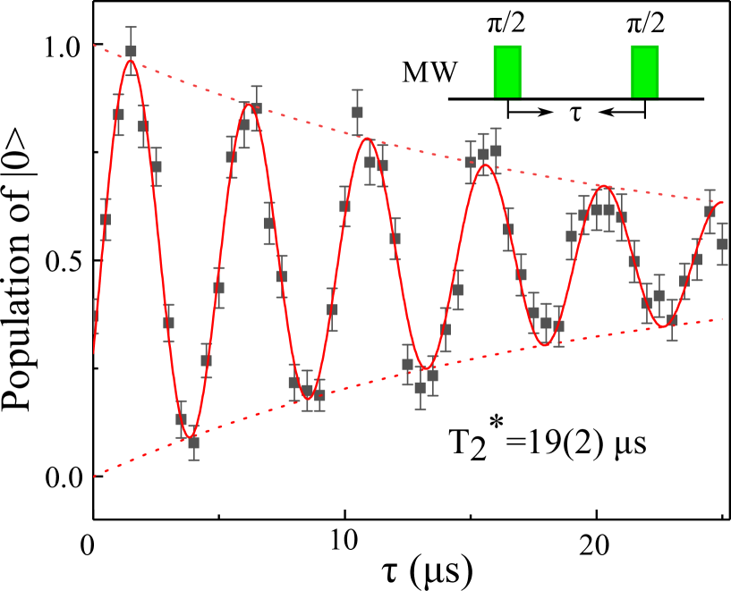
Figure S3: Coherence time of NV center. Result of the Ramsey experiment (insert, pulse sequence) for the electron spin. The solid red line is fit to the experiment data (black square), the red dashed line is the fit to the envelope curve. The decay time of FID is measured to be $T_{2}^{\star}=19(2)~{}\mathrm{\mu s}$.

VI VI. Nuclear spin qubit operation

The single qubit operations of the nuclear spin qubit in the state prepartion and read out are realized by applying two channel radio frequency (RF) pulses simultaneously. The frequencies of the RF pulses are $2.9~{}\mathrm{MHz}$ and $5.1~{}\mathrm{MHz}$, corresponding to the nuclear spin transition frequencies. The RF pulses are generated by AWG and then carried by a homebuild RF coil with dual resonance frequencies. The coil is designed according to ref.[Dissertation_Dabirzadeh, ]. There are two input ports at the coil to input the RF pulses, and the return loss of the two ports is shown in Fig. S4. The Rabi frequencies of the nuclear spin transitions at different electron subspace are both calibrated to be 25 $\mathrm{kHz}$.

Figure S4: Return loss of the RF Coil. Return loss of the RF coil, red line stands for the low frequency port, at $2.9~{}\mathrm{MHz}$, the return loss is $-9.1~{}\mathrm{dB}$, bule line stands for the high frequency port, at $5.1~{}\mathrm{MHz}$, the retirn loss is $-6.5~{}\mathrm{dB}$.

References

(1) Bender, C. M. Boettcher, S. Real spectra in non-Hermitian Hamiltonians having PT symmetry. Phys. Rev. Lett.80, 5243 (1998).
(2) Bender, C. M., Brody, D. C. Jones, H. F. Complex extension of quantum mechanics. Phys. Rev. Lett.89, 270401 (2002).
(3) Bender, C. M. Making sense of non-Hermitian Hamiltonians. Rep. Prog. Phys.70, 947 (2007).
(4) Rter, C. E. et al. Observation
of parity-time symmetry in optics. Nat. Phys.6, 192
(2010).
(5) Bender, N. et al. Observation of asymmetric transport in structures with active nonlinearities. Phys. Rev. Lett.110, 234101 (2013).
(6) Assawaworrarit, S., Yu, X. Fan, S. Robust wireless power transfer using a nonlinear parity-time-symmetric circuit. Nature546, 387 (2017).
(7) Choi, Y., Hahn, C., Yoon, J. W. Song, S. H. observation of an anti-PT-symmetric exceptional point and energy-difference conserving dynamics in electrical circuit resonators. Nat. Commun.9, 2182 (2018).
(8) Bittner, S. et al. PT symmetry and spontaneous symmetry breaking in a microwave billiard. Phys. Rev. Lett.108, 024101 (2012).
(9) Bender, C. M., Berntson, B. K., Parker, D. Samuel, E. Observation of PT phase transition in a simple mechanical system. Am. J. Phys.81, 173 (2013).
(11) Popa, B.-I. Cummer, S. A. Non-reciprocal and highly nonlinear active acoustic metamaterials. Nat. Commun.5, 3398 (2014).
(12) Fleury, R., Sounas, D. Al, A. An invisible acoustic sensor based on parity-time symmetry. Nat. Commun.6, 5905 (2015).
(13) El-Ganainy, R. et al. Non-Hermitian physics and PT symmetry. Nat. Phys.14, 11 (2018).
(14) Hang, C., Huang, G. Konotop, V. V. PT symmetry with a system of three-level atoms. Phys. Rev. Lett.110, 083604 (2013).
(15) Peng, P. et al. Anti-parity-time symmetry with flying atoms. Nat. Phys.12, 1139 (2016).
(16) Zhang, Z. et al. Observation of parity-time symmetry in optically induced atomic lattices. Phys. Rev. Lett.117, 123601 (2016).
(17) Cham, J. Top 10 physics discoveries of the last 10 years. Nat. Phys.11, 799 (2015).
(18) Feng, L. et al. Nonreciprocal light propagation in a silicon photonic circuit. Science333, 729 (2011).
(19) Peng, B. et al. Parity-time-symmetric whispering-gallery microcavities. Nature Phys.10, 394 (2014).
(20) Feng, L., Wong, Z. J., Ma, R.-M., Wang, Y. Zhang, X. Single-mode laser by parity-time symmetry breaking. Science346, 972 (2014).
(21) Hodaei, H., Miri, M.-A., Heinrich, M., Christodoulides, D. N. Khajavikhan, M. Parity-time-symmetric microring lasers. Science346, 975 (2014).
(22) Gardas, B., Deffner, S. Saxena, A. PT-symmetric slowing down of decoherence. Phys. Rev. A94, 040101 (2016).
(23) Gao, T. et al. Observation of non-Hermitian degeneracies in a chaotic exciton-polariton billiard. Nature526, 554 (2015).
(24) Zhang, D., Luo, X.-Q., Wang, Y.-P., Li, T.-F. You, J.Q. Observation of the exceptional point in cavity magnon-polaritons. Nature Commun.8, 1368 (2017).
(25) Li, J. et al. Observation of parity-time symmetry breaking transitions in a dissipative Floquet system of ultracold atoms. arXiv: 1608.05061.
(26) Tang, J.-S. et al. Experimental investigation of the no-signalling principle in parity-time symmetric theory using an open quantum system. Nature Photon.10, 642 (2016).
(27) Xiao, L. et al. Observation of topological edge states in parity-time-symmetric quantum walks. Nature Phys.13, 1117 (2017).
(28) Gnther, U. Samsonov, B. F. Naimark-dilated PT-symmetric brachistochrone. Phys. Rev. Lett.101, 230404 (2008).
(29) Kawabata, K., Ashida, Y. Ueda, M. Information retrieval and criticality in parity-time-symmetric systems. Phys. Rev. Lett.119, 190401 (2017).
(30) Jacques, V. et al. Dynamic polarization of single nuclear spins by optical pumping of nitrogen-vacancy color centers in diamond at room temperature. Phys. Rev. Lett.102, 057403 (2009).

References

(1) M.Steiner, P.Neumann, et al. Universal Enhancement of the optical readout fidelity of single electron spins at nitrogen-vacancy centers in diamond. Phys. Rev. B81, 035205 (2010).
(2) V.Jacques, P.Neumann et al. Dynamic Polarization of Single Nuclear Spin by Optical Pumping of Nitrogen-Vacancy Color Centers in Diamonds at room temperature. Phys. Rev. Lett.102, 057403 (2009).
(3) A.Dabirzadeh, RF coil design for multi-frequency magnitic resonance imaging and spectroscopy. Texas, AM university, December 2008.