Two-neutron transfer reactions and shape phase transitions in the microscopically-formulated interacting boson model

Abstract

Two-neutron transfer reactions are studied within the interacting boson model based on the nuclear energy density functional theory. Constrained self-consistent mean-field calculations with the Skyrme energy density functional are performed to provide microscopic input to completely determine the Hamiltonian of the IBM. Spectroscopic properties are calculated only from the nucleonic degrees of freedom. This method is applied to study the $(t,p)$ and $(p,t)$ transfer reactions in the assorted set of rare-earth nuclei ^146-158Sm, ^148-160Gd, and ^150-162Dy, where spherical-to-axially-deformed shape phase transition is suggested to occur at the neutron number $N\approx 90$. The results are compared with those from the purely phenomenological IBM calculations, as well as with the available experimental data. The calculated $(t,p)$ and $(p,t)$ transfer reaction intensities, from both the microscopic and phenomenological IBM frameworks, signal the rapid nuclear structural change at particular nucleon numbers.

I Introduction

The simultaneous theoretical description of nuclear structure and reaction is one of the ultimate goals of low-energy nuclear physics. At experiment nucleon-pair transfer reactions are instrumental for studying variety of nuclear structure phenomena. Of particular interest here is the shape phase transition Cejnar and Jolie (2009); Cejnar et al. (2010); Iachello (2011); Carr (2010), where nuclear shape/structure changes as a function of nucleon number and which is identified as an abrupt change of observables that are considered the order parameters of the phase transition. For many decades the two-nucleon transfer reactions, especially the $(t,p)$ and $(p,t)$ ones, have been used to study rapid structural evolution from one nuclear structure to another Maxwell et al. (1966); Bjerregaard et al. (1966); Fleming et al. (1971); Casten et al. (1972); Fleming et al. (1973); Shahabuddin et al. (1980); Løvhøiden et al. (1986, 1989); Lesher et al. (2002) and, in that context, explored by a number of empirical theoretical models Fossion et al. (2007); Clark et al. (2009); Zhang and Iachello (2017); Cejnar et al. (2010).

The Interacting Boson Model (IBM) Iachello and Arima (1987), a model where correlated nucleon pairs are represented by bosonic degrees of freedom, has been remarkably successful in the phenomenological description of low-energy collective excitations in medium-heavy and heavy nuclei. The microscopic foundation of the IBM, starting from nucleonic degrees of freedom, has been explored for decades Otsuka et al. (1978a, b); Mizusaki and Otsuka (1996); Nomura et al. (2008, 2011). Among these studies, a comprehensive method to derive the Hamiltonian of the IBM has been developed in Ref. Nomura et al. (2008). In this method, potential energy surface (PES) in the quadrupole deformation space is calculated within the constrained self-consistent mean-field (SCMF) method with a choice of energy density functional (EDF), and is mapped onto the expectation value of the IBM Hamiltonian in the boson coherent state Ginocchio and Kirson (1980). This procedure uniquely determines the strength parameters of the IBM Hamiltonian. For strongly-deformed nuclei in particular, rotational response of the nucleonic intrinsic state has been incorporated microscopically in the IBM framework, and this has allowed for calculating the rotational spectra of deformed nuclei accurately Nomura et al. (2011). Since the EDF framework provides a global mean-field description of various low-energy properties of the nuclei over the entire region of the nuclear chart, it has become possible to derive the IBM Hamiltonian for any arbitrary nuclei in a unified way.

In this article, we present a first application of the SCMF-to-IBM mapping procedure of Refs. Nomura et al. (2008, 2011) to the nucleon-pair transfer reactions as a signature of the shape phase transitions. We demonstrate how the method works for the description of the transfer reactions, in the applications to the rare-earth nuclei ^146-158Sm, ^148-160Gd, and ^150-162Dy, which are an excellent example of the spherical-to-axially-deformed shape phase transition Cejnar et al. (2010). To the best of our knowledge, ever since its first application in 1977 Arima and Iachello (1977), the IBM has not been used as extensively to describe nuclear reactions, including the two-nucleon transfer reactions, which involve different nuclei, as the spectroscopy in a single nucleus. There are a few recent examples where the IBM was used in phenomenological studies of $(t,p)$ and $(p,t)$ reactions Fossion et al. (2007); Pascu et al. (2009, 2010); Zhang and Iachello (2017).

Already in Ref. Kotila et al. (2012), key spectroscopic properties of the above-mentioned Gd and Dy nuclei, i.e., energies and electromagnetic transition rates, that signal the first-order phase transition, were studied within the SCMF-to-IBM mapping procedure using the Skyrme SkM* J. Bartel et al. (1982) EDF and were compared with the purely phenomenological IBM calculation. The main conclusion of that study was that the shape transition as a function of the neutron number $N$ occurred rather moderately in the microscopically-formulated IBM, as compared to the phenomenological IBM calculation Kotila et al. (2012).

Here we have made somewhat a similar analysis to the one in Kotila et al. (2012), that is, compared the $(p,t)$ and $(t,p)$ transfer reaction intensities obtained from the SCMF-to-IBM mapping procedure with those from the phenomenological IBM calculation of Ref. Kotila et al. (2012). In addition, we also compare our results with a more recent, extensive IBM study for the $(t,p)$ and $(p,t)$ transfer reactions in the same mass region Zhang and Iachello (2017). In this way, we shall examine the robustness of the IBM framework on the pair-transfer reactions and shape phase transitions.

In Sec. II we describe the theoretical methods. The calculated potential energy surfaces, excitation spectra, and $(p,t)$ and $(t,p)$ transfer reaction intensities for the considered nuclei are presented in Sec. III, followed by a concise summary and concluding remarks in Sec. IV.

II Theoretical tools

Firstly we briefly describe the SCMF-to-IBM mapping procedure, together with the two other phenomenological IBM calculations, which have been employed in the present work. More detailed accounts of the employed theoretical methods have been already given in Refs. Nomura et al. (2010, 2011); Kotila et al. (2012); Zhang and Iachello (2017), and the reader is referred to that literature.

II.1 SCMF-to-IBM mapping

In the present analysis we used the neutron-proton IBM (IBM-2), which distinguishes both neutron and proton degrees of freedom Otsuka et al. (1978b). The IBM-2 is comprised of the neutron (proton) monopole $s_{\nu}$ ($s_{\pi}$) and quadrupole $d_{\nu}$ ($d_{\pi}$) bosons, which represent, from a microscopic point of view, the collective pairs of valence neutrons (protons) with spin and parity $0^{+}$ and $2^{+}$, respectively Otsuka et al. (1978b). The number of neutron (proton) bosons, denoted by $N_{\nu}$ ($N_{\pi}$), is equal to that of the neutron (proton) pairs. In this work the doubly-magic nucleus ¹³²Sn has been taken as an inert core. Hence $1\leq N_{\nu}\leq 7$, and $N_{\pi}=6$ (for ^146-158Sm), $N_{\pi}=7$ (for ^148-160Gd), and $N_{\pi}=8$ (for ^150-162Dy). For the IBM-2 Hamiltonian we employed the following form:

$$\hat{H}=\epsilon(\hat{n}_{d_{\nu}}+\hat{n}_{d_{\pi}})+\kappa\hat{Q}_{\nu}\cdot\hat{Q}_{\pi}+\kappa^{\prime}\hat{L}\cdot\hat{L},$$ (1)

where $\hat{n}_{d_{\rho}}=d^{\dagger}_{\rho}\cdot\tilde{d}_{\rho}$ ($\rho=\nu,\pi$) is the $d$-boson number operator, $\hat{Q}_{\rho}=d_{\rho}^{\dagger}s_{\rho}+s_{\rho}^{\dagger}\tilde{d}_{\rho}+\chi_{\rho}(d^{\dagger}_{\rho}\times\tilde{d}_{\rho})^{(2)}$ is the quadrupole operator, and $\hat{L}=\hat{L}_{\nu}+\hat{L}_{\pi}$ is the angular momentum operator with $\hat{L}_{\rho}=\sqrt{10}(d_{\rho}^{\dagger}\times\tilde{d}_{\rho})^{(1)}$. $\epsilon$, $\kappa$, $\chi_{\nu}$, $\chi_{\pi}$, and $\kappa^{\prime}$ are the parameters.

As the first step of determining the IBM-2 Hamiltonian, we carried out for each considered nucleus the constrained SCMF calculation within the Hartree-Fock+BCS method Bonche et al. (2005) based on the Skyrme SkM* EDF J. Bartel et al. (1982) to obtain PES with the quadrupole $(\beta,\gamma)$ shape degrees of freedom. The constraint is that of the mass quadrupole moment and, for the pairing correlation, the density-dependent $\delta$-type pairing force has been used with the strength of 1250 MeV fm³.

The SCMF PES thus obtained has been mapped onto the expectation value of the IBM-2 Hamiltonian in the boson coherent state Ginocchio and Kirson (1980), and this procedure completely determined the parameters $\epsilon$, $\kappa$, $\chi_{\nu}$, and $\chi_{\pi}$ Nomura et al. (2008, 2010). Only the strength parameter $\kappa^{\prime}$ for the $\hat{L}\cdot\hat{L}$ term has been determined separately from the other parameters, by adjusting the cranking moment of inertia in the boson intrinsic state to the corresponding cranking moment of inertia computed within the SCMF calculation at the equilibrium mean-field minimum Nomura et al. (2011). No phenomenological adjustment of the parameters to experiment was made in the whole procedure. We used the same values of the parameters as used in Ref. Nomura et al. (2010) for the Sm isotopes and Ref. Kotila et al. (2012) for the Gd and Dy isotopes.

Energy spectra and electromagnetic transition rates have been obtained by the $m$-scheme diagonalization of the mapped IBM-2 Hamiltonian Nomura (2012), and the resulting wave functions have been used to calculate the $(t,p)$ and $(p,t)$ transfer reaction intensities. In this work, as in Zhang and Iachello (2017), we only considered the $(t,p)$ and $(p,t)$ transfers of the monopole and quadrupole pairs of neutrons within each isotopic chain. The corresponding $(t,p)$ and $(p,t)$ transfer operators, denoted by $\hat{P}^{(L)}_{+}$ and $\hat{P}^{(L)}_{-}$ (with $L=0$ or $2$), respectively, can be expressed as Arima and Iachello (1977); Iachello and Arima (1987):

$$\hat{P}^{(0)}_{+}=(\hat{P}^{(0)}_{-})^{(\dagger)}=t_{0}s^{\dagger}_{\nu}A(\Omega_{\nu},N_{\nu})$$ (2)

$$\hat{P}^{(2)}_{+}=(\hat{P}^{(2)}_{-})^{(\dagger)}=t_{2}d^{\dagger}_{\nu}A(\Omega_{\nu},N_{\nu}),$$ (3)

The factor $A(\Omega_{\nu},N_{\nu})$ in Eqs. (2) and (3) is given by

$$A(\Omega_{\nu},N_{\nu})=\sqrt{\Omega_{\nu}-N_{\nu}-\hat{n}_{d_{\nu}}},$$ (4)

with $\Omega_{\nu}$ the degeneracy of the neutron pairs in a given major shell, i.e., $\Omega_{\nu}=(126-82)/2=22$ in the considered nuclei. For the sake of simplicity, the operator $\hat{n}_{d_{\nu}}$ in Eq. (4) has been replaced with its expectation value in the ground state of the initial nucleus, i.e., $\langle\hat{n}_{d_{\nu}}\rangle_{0^{+}_{1}}$ Fossion et al. (2007). $t_{0}$ and $t_{2}$ in the same equation are overall scale factors. The intensities of the $(t,p)$ and $(p,t)$ transfer reactions are given, respectively, as:

$$I^{\rm(tp)}(N,J_{i}\to N+2,J_{f})$$

$$=\frac{1}{2J_{i}+1}|\langle N+2,J_{f}||\hat{P}_{+}^{(L)}||N,J_{i}\rangle|^{2}$$ (5)

and

$$I^{\rm(pt)}(N+2,J_{i}\to N,J_{f})$$

$$=\frac{1}{2J_{i}+1}|\langle N,J_{f}||\hat{P}_{-}^{(L)}||N+2,J_{i}\rangle|^{2},$$ (6)

where the state $|N,J_{i,f}\rangle$ represents the IBM-2 wave function for a nucleus with the neutron number $N$ and total angular momentum $J_{i}$ for the initial or $J_{f}$ for the final states. Here we considered the transfer reactions from the $0^{+}_{1}$ ground state of the initial nucleus to the lowest three $0^{+}$ and $2^{+}$ states of the final nucleus.

In what follows, the mapped IBM-2 framework, described in this section, is referred to as $m$-IBM .

Figure 1: Potential energy surfaces for the nuclei ^148-154Sm plotted within the $(\beta,\gamma)$ deformation space and with up to 5 MeV from the global minimum. The energy difference between neighboring contours is 250 keV. See the main text for details.

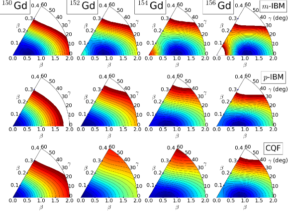
Figure 2: Same as for Fig. 1, but for the nuclei ^150-156Gd.

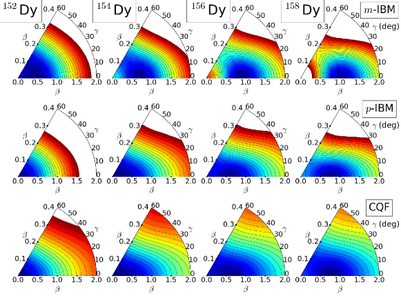
Figure 3: Same as for Fig. 1, but for the nuclei ^152-158Dy.

II.2 Phenomenological IBM-2

Along with the $m$-IBM calculation we have carried out the purely phenomenological IBM-2 calculations using the same Hamiltonian as in Eq. (1), but with parameters adjusted to reproduce low-energy spectra for each considered nucleus. The fitted parameters for the Sm isotopes are presented in Table 1. The parameters for the nuclei ¹⁵⁰Sm and ¹⁵²Sm have been taken from Ref. Scholten (1980). For the Gd and Dy isotopes, we employed the same values of the parameters $\epsilon$, $\kappa$, $\chi_{\nu}$, and $\chi_{\pi}$ as those used in Ref. Kotila et al. (2012). The IBM-2 Hamiltonian considered in Ref. Kotila et al. (2012) was comprised, in addition to the three terms in the above Hamiltonian in Eq. (1), those proportional to $(d_{\rho}^{\dagger}\times d_{\rho}^{\dagger})^{(L)}\cdot(\tilde{d}_{\rho}\times\tilde{d}_{\rho})^{(L)}$ with $L=0$ and 2, and the so-called Majorana terms. In the present calculation, these terms have not been included, as they play only a minor role in the description of the low-lying states. The $(t,p)$ and $(p,t)$ transfer operators were already defined in Eqs. (2)–(II.1).

We denote, hereafter, the purely phenomenological IBM-2 calculation thus far mentioned as $p$-IBM , unless otherwise specified.

Table 1: The $p$-IBM parameters of the IBM-2 Hamiltonian in Eq. (1) for the nuclei ^146-158Sm, determined in this study so as to reproduce the experimental low-lying spectra. The value of the parameter $\kappa^{\prime}$ has been taken to be zero for all the Sm nuclei.

	146Sm	148Sm	150Sm	152Sm	154Sm	156Sm	158Sm
$\epsilon$ (MeV)	1.100	1.000	0.700	0.520	0.450	0.400	0.400
$\kappa$ (MeV)	-0.140	-0.130	-0.080	-0.075	-0.085	-0.085	-0.085
$\chi_{\nu}$	-0.800	-1.000	-0.800	-1.000	-1.200	-1.200	-1.200
$\chi_{\pi}$	-0.800	-1.000	-1.300	-1.300	-1.200	-1.200	-1.200

II.3 IBM-1 in the consistent-Q formalism

We have also performed a similar phenomenological calculation within the IBM-1, where no distinction is made between neutron and protons bosons. We adapted the same Hamiltonian in the so-called consistent-Q formalism (CQF) Warner and Casten (1983) as the one used in Ref. Zhang and Iachello (2017). The CQF Hamiltonian reads:

$$\hat{H}_{\text{CQF}}=\epsilon_{0}\Big{[}(1-\eta)\hat{n}_{d}-\frac{\eta}{4N}\hat{Q}^{\chi}\cdot\hat{Q}^{\chi}\Big{]}.$$ (7)

$\eta$ and $\chi$ (which appears in the quadrupole operator $\hat{Q}$) are the control parameters, and $\epsilon_{0}$ is the scale factor fitted to reproduce the $2^{+}_{1}$ excitation energy for each nucleus. The $(t,p)$ and $(t,p)$ transfer operators in the IBM-1 framework are similar to the IBM-2 counterparts in Eqs. (2)–(II.1), except for the factor $A(\Omega_{\nu},N_{\nu})$. For all the details of the CQF calculation, the reader is referred to Ref. Zhang and Iachello (2017). For the calculations on the Sm and Gd isotopes, the same parameters as in Ref. Zhang and Iachello (2017) have been used. Only for the Dy isotopes, the calculation has been newly made, and the values of the control parameters $\eta$ and $\chi$ for the Hamiltonian $\hat{H}_{\text{CQF}}$ have been taken from the earlier IBM-1 study on the rare-earth nuclei in Ref. McCutchan et al. (2004) and are listed in Table 2.

Table 2: Control parameters of the Hamiltonian $\hat{H}_{\text{CQF}}$ in Eq. (7) determined in this study for the isotopes ^150-162Dy.

	150Dy	152Dy	154Dy	156Dy	158Dy	160Dy	162Dy
$\eta$	0.1	0.35	0.49	0.62	0.71	0.81	0.92
$\chi$	-1.12	-1.10	-1.09	-0.85	-0.67	-0.49	-0.31

III Results and discussions

III.1 Potential energy surface

In Figs. 1, 2, and 3 plotted are the PESs within the $(\beta,\gamma)$-deformation space for the studied nuclei ^148-154Sm, ^150-156Gd, and ^152-158Dy, respectively. In these figures, the $m$-IBM , $p$-IBM , and CQF PESs are compared with each other. Note that the PESs for the $N=84$ and 96 nuclei in each isotopic chain have not been plotted in the figures, since they turned out to be strikingly similar to those for their neighbouring isotopes with $N=86$ and 94, respectively. Here we mainly discuss the PESs for the Sm isotopes, whereas we confirmed that the main conclusions were basically the same for the Gd and Dy isotopes.

There is an anzats that the deformation parameter $\beta$ in the IBM can be related to the one in the geometrical collective model, denoted as $\bar{\beta}$, in such a way that they are proportional to each other, i.e., $\beta=C_{\beta}\bar{\beta}$ Ginocchio and Kirson (1980), where $C_{\beta}$ is the scaling factor and typically takes values $C_{\beta}\approx 3-5$ in the rare-earth region Nomura et al. (2008). In the $m$-IBM framework, the coefficient $C_{\beta}$ has been explicitly determined by the mapping. In Figs. 1, 2, and 3, however, the $m$-IBM PESs are drawn in terms of the $\beta$ deformation in the IBM, in order that one can directly compare them with the $p$-IBM and CQF PESs.

In general, from Figs. 1, 2, and 3, the PESs in the $m$-IBM turned out to be more strongly deformed and suggested less striking change in topology as functions of $N$ than those obtained from the $p$-IBM and CQF Hamiltonians. In Fig. 1 the $m$-IBM PES for the nucleus ¹⁴⁸Sm exhibits a nearly spherical mean-field minimum around $\beta=0.5$. In the same figure, one sees that the location of the minimum, denoted as $\beta_{\rm min}$, in the $m$-IBM PES jumps from ¹⁴⁸Sm ($\beta_{\rm min}\approx 0.5$) to ¹⁵⁰Sm ($\beta_{\rm min}\approx 1.0$). The latter nucleus is suggested to be already well deformed in the $m$-IBM calculation. For the ^152,154Sm nuclei, one sees even more pronounced prolate minimum at $\beta\approx 1.0$, i.e., deeper in energy in both $\beta$ and $\gamma$ directions, in the corresponding $m$-IBM PESs. On the other hand, the $p$-IBM PESs, depicted in the middle row of Fig. 1, exhibit a more dramatic change in its topology as a function of $N$: spherical minimum at $\beta=0$ at ¹⁴⁸Sm, weakly prolate deformed minimum at ¹⁵⁰Sm, softer minimum in both $\beta$ and $\gamma$ directions at ¹⁵²Sm characteristic of the critical-point nucleus, and well developed prolate minimum at ¹⁵⁴Sm. There is no noticeable difference between the PESs obtained from the $p$-IBM and CQF Hamiltonians.

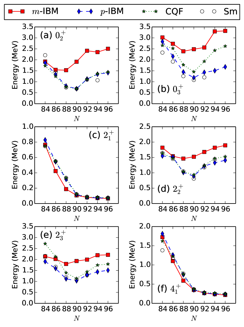
Figure 4: (Color online) Excitation energies of the low-lying states $0^{+}_{2}$ (a), $0^{+}_{3}$ (b), $2^{+}_{1}$ (c), $2^{+}_{2}$ (d), $2^{+}_{3}$ (e), and $4^{+}_{1}$ (f) for the ^150-158Sm isotopes are plotted against the neutron number $N$. The results of the three versions of the IBM calculations, i.e., $m$-IBM , $p$-IBM , and CQF, are compared with each other and with the experimental data Brookhaven National Nuclear Data Center .

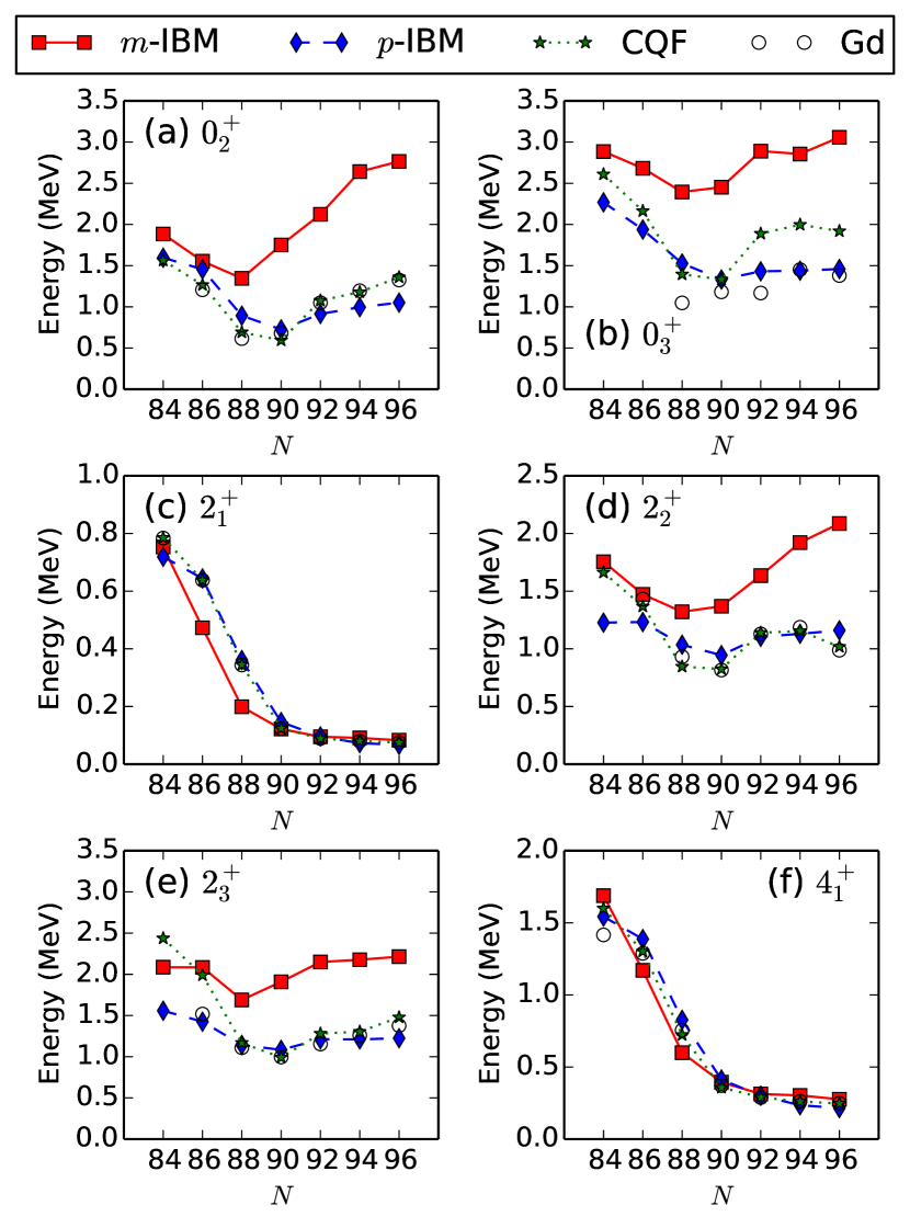
Figure 5: (Color online) Same as Fig. 4, but for the ^148-160Gd isotopes.

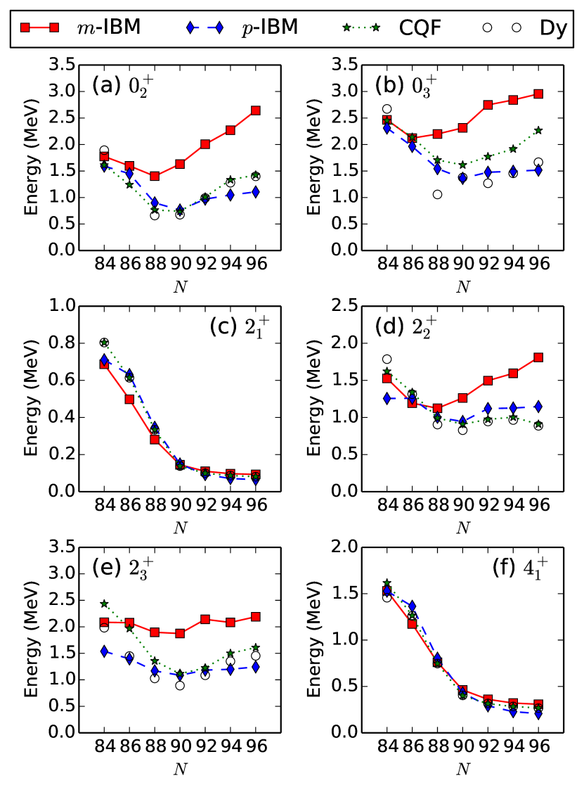
Figure 6: (Color online) Same as Fig. 4, but for the ^150-162Dy isotopes.

III.2 Excitation energies

As a reminder of the results in Refs. Nomura et al. (2010); Kotila et al. (2012); Zhang and Iachello (2017), we plotted in Figs. 4, 5, and 6 the excitation energies of the low-lying states in the ^146-158Sm, ^148-160Gd, and ^150-162Dy isotopes, respectively, that are relevant to the $(t,p)$ and $(p,t)$ transfer reactions studied in this work.

III.2.1 Sm isotopes

In Fig. 4 we display the calculated excitation energies of Sm isotopes. The shape phase transition can be identified by the sharp parabolic systematics of both the $0^{+}_{2}$ and $0^{+}_{3}$ energy levels centered around $N=90$, corresponding to the X(5) critical-point nucleus ¹⁵²Sm Casten and Zamfir (2001). But in the $m$-IBM results, the $0^{+}_{2}$ and $0^{+}_{3}$ energy levels become lowest rather at $N=88$. Both phenomenological ($p$-IBM and CQF) calculations reproduced the experimental $0^{+}_{2}$ and $0^{+}_{3}$ energy levels very well, while the IBM-2 description looks slightly better than the IBM-1 one. In the $m$-IBM , evolution of the energy levels generally looks more moderate than in the other two calculations. Moreover, both the non-yrast $0^{+}_{2}$ and $0^{+}_{3}$ energies were overestimated by the $m$-IBM calculation. This most likely traces back to the fact that the underlying SCMF PESs suggested a too deformed mean-field minimum Nomura et al. (2010) and that the corresponding mapped IBM-2 produced a rather rotational energy spectrum. Almost the same conclusion as for the results of the non-yrast $0^{+}$ states can be reached in the comparisons of the $2^{+}_{2}$ (Fig. 4(d)) and $2^{+}_{3}$ (Figs. 4(e)) energy levels.

In Fig. 4(c), the $2^{+}_{1}$ energy level has been reproduced very well by the three calculations. But for the transitional nuclei, i.e., ¹⁵⁰Sm ($N=88$) and ¹⁵²Sm ($N=90$), it has been predicted to be too low in energy in the $m$-IBM , suggesting rather deformed energy spectra.

As seen from Fig. 4(f), the three IBM calculations reproduced very nicely the experimental $4^{+}_{1}$ energy level. However, for the nucleus ¹⁴⁶Sm in particular, the calculations could not account for the low-lying $4^{+}_{1}$ state, resulting in the predicted energy ratio $R\equiv E(4^{+}_{1})/E(2^{+}_{1})$ that is below the vibrational limit, i.e., $R<2$. This is mainly because of the limited configuration space used in the present version of the IBM, that is built only on the collective $s$ and $d$ bosons.

III.2.2 Gd isotopes

In the Gd isotopic chain, the experimental $0^{+}_{2}$ energy level, shown in Fig. 5(a), exhibits parabolic behaviour, being lowest in energy at $N=88$. The $m$-IBM result followed this systematics nicely, but systematically overestimated the data, due to the same reasons as we discussed in the previous section. The $p$-IBM and CQF calculations provided an excellent description of the data but, at variance with the $m$-IBM result and the experiment, suggested that the $0^{+}_{2}$ level was lowest at $N=90$.

Compared to the results for the Sm isotopes, as seen from Fig. 5(b) the experimental $0^{+}_{3}$ energy level in Gd does not show a significant, but rather irregular, $N$ dependence for $88\leq N\leq 96$. Specially the $p$-IBM calculation reproduced this trend fairly well. However, the agreement with the experimental data in the $0^{+}_{3}$ excitation energies appears to be not as good as in the $0^{+}_{2}$ ones (Fig. 5(a)), even in the phenomenological $p$-IBM and CQF calculations. Let us recall that the low-lying $0^{+}$ excited states in Gd and Dy isotopes have often been attributed to additional degrees of freedom, such as intruder excitations, which are beyond the configuration spaces considered in the present IBM framework.

Both the $2^{+}_{1}$ (Fig. 5(c)) and $4^{+}_{1}$ (Fig. 5(f)) excitation energies have been nicely described by the three calculations. As seen from Figs. 5(d) and 5(e), the phenomenological IBM calculations reproduced the non-yrast $2^{+}$ levels, but the $m$-IBM overestimated them.

III.2.3 Dy isotopes

The main conclusion from the comparisons between the theoretical and experimental excitation spectra for the Dy isotopes in Fig. 6 turned out be basically the same as for the Gd nuclei, discussed in the previous section. Namely: The $m$-IBM overestimated the experimental data for the non-yrast states, and differed in the predicted energy-level systematics from the $p$-IBM and CQF ones; The experimental $0^{+}_{3}$ energy level exhibits rather irregular systematics against $N$, and this experimental trend was not accounted for by the present version of the IBM comprising only collective $s$ and $d$ bosons.

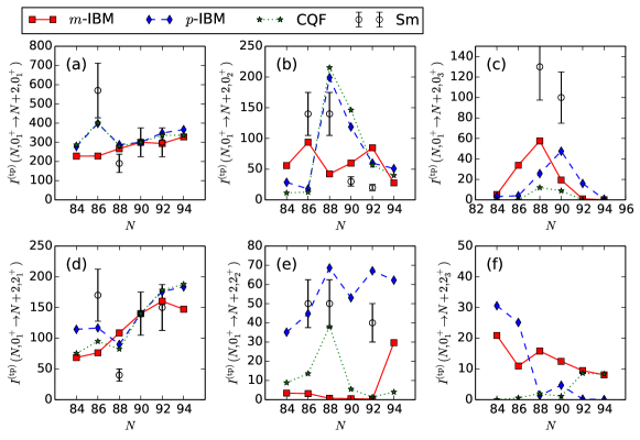
Figure 7: (Color online) The $(t,p)$ transfer reaction intensities for the ^146-156Sm isotopes. The results of the $m$-IBM, $p$-IBM, and CQF calculations are compared with each other and with the experimental data Bjerregaard et al. (1966). The scale factors $t_{0}$ and $t_{2}$ in the $(t,p)$ transfer operators have been fitted to the experimental data for the $0^{+}_{1}(^{152}{\rm Sm})\to 0^{+}_{1}(^{154}$Sm) and $0^{+}_{1}(^{152}{\rm Sm})\to 2^{+}_{1}(^{154}$Sm) transfer reactions, respectively.

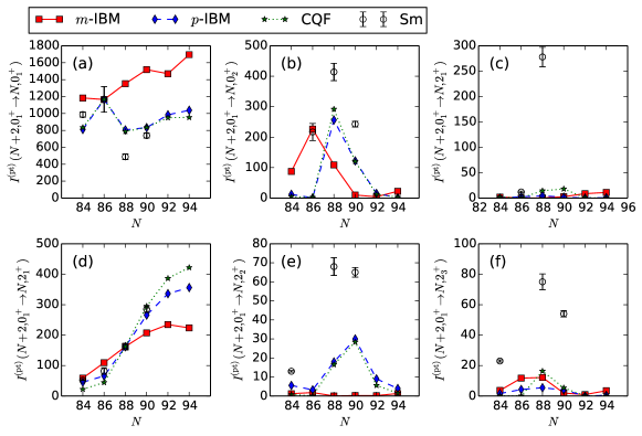
Figure 8: (Color online) Similar to Fig. 7, but for the $(p,t)$ transfer reaction intensities for the ^146-156Sm isotopes. The experimental data have been taken from Ref. Debenham and Hintz (1972). The scale factors $t_{0}$ and $t_{2}$ in the $(p,t)$ transfer operators have been fitted to the experimental data for the $0^{+}_{1}(^{150}{\rm Sm})\to 0^{+}_{1}(^{148}$Sm) and $0^{+}_{1}(^{152}{\rm Sm})\to 2^{+}_{1}(^{150}$Sm) transfer reactions, respectively.

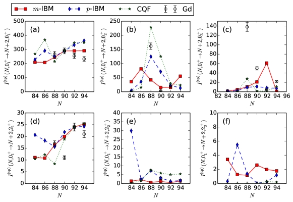
Figure 9: (Color online) Same as Fig. 7, but for the ^158-158Gd isotopes. The experimental data have been taken from Refs. Shahabuddin et al. (1980); Løvhøiden et al. (1989, 1986). The scale factors $t_{0}$ and $t_{2}$ have been fitted to the experimental data for the $0^{+}_{1}(^{154}{\rm Gd})\to 0^{+}_{1}(^{156}$Gd) and $0^{+}_{1}(^{156}{\rm Gd})\to 2^{+}_{1}(^{158}$Gd) transfer reactions, respectively.

Figure 10: (Color online) Same as Fig. 8, but for the ^158-158Gd isotopes. The experimental data have been taken from Ref. Fleming et al. (1973). The scale factors $t_{0}$ and $t_{2}$ have been fitted to the experimental data for the $0^{+}_{1}(^{156}{\rm Gd})\to 0^{+}_{1}(^{154}$Gd) and $0^{+}_{1}(^{154}{\rm Gd})\to 2^{+}_{1}(^{152}$Gd) transfer reactions, respectively.

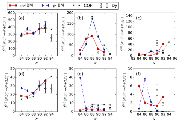
Figure 11: (Color online) Same as Fig. 7, but for the ^150-160Dy isotopes. The experimental data have been taken from Ref. Burke et al. (1988). The scale factors $t_{0}$ and $t_{2}$ have been fitted to the experimental data for the $0^{+}_{1}(^{156}{\rm Dy})\to 0^{+}_{1}(^{158}$Dy) and $0^{+}_{1}(^{156}{\rm Dy})\to 2^{+}_{1}(^{158}$Dy) transfer reactions, respectively.

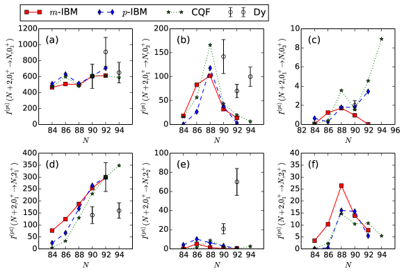
Figure 12: (Color online) Same as Fig. 8, but for the ^150-160Dy isotopes. The experimental data have been taken from Ref. Kolata and Oothoudt (1977) for ¹⁵⁸Dy$(p,t)^{156}$Dy and Ref. Maher et al. (1972) for ¹⁶²Dy$(p,t)^{160}$Dy and ¹⁶⁰Dy$(p,t)^{158}$Dy reactions. The scale factors $t_{0}$ and $t_{2}$ have been fitted to the experimental data for the $0^{+}_{1}(^{158}{\rm Dy})\to 0^{+}_{1}(^{156}$Dy) and $0^{+}_{1}(^{160}{\rm Dy})\to 2^{+}_{1}(^{158}$Dy) transfer reactions, respectively.

III.3 $(t,p)$ and $(p,t)$ transfer reactions

Let us now turn to the discussions about the $(t,p)$ and $(p,t)$ transfer reactions. As in the earlier IBM calculations for the two-nucleon transfer reactions Arima and Iachello (1977); Scholten (1980); Zhang and Iachello (2017), we compare the calculated $(t,p)$ and $(p,t)$ transfer intensities with the experimental cross sections measured at particular laboratory angles. To facilitate the comparisons, we have determined the overall scale factors $t_{0}$ and $t_{2}$ in the transfer operators (see, Eqs. (2) and (3)) so as to reproduce the experimental $0^{+}_{1,i}\to 0^{+}_{1,f}$ and $0^{+}_{1,i}\to 2^{+}_{1,f}$ transfer reaction cross sections at given angles for particular nuclei. More details are mentioned in the captions to Figs. 7 – 12.

III.3.1 Sm isotopes

We show in Figs. 7 and 8 the calculated $(t,p)$ and $(p,t)$ transfer reaction intensities for the Sm isotopes as functions of $N$. The experimental data, available in Refs. Bjerregaard et al. (1966); Debenham and Hintz (1972), are also included in the plot.

In Fig. 7, for many of the $(t,p)$ transfer reactions the $m$-IBM results exhibit a certain discontinuity around particular nucleus in the transitional region. In general, the $(t,p)$ reaction rates resulting from the $m$-IBM did not exhibit change with $N$ as rapid as those from the $p$-IBM and CQF and, in some reactions, show completely different $N$ dependence from the latter. A typical example is the $I^{\rm(tp)}(N,0^{+}_{1}\to N+2,0^{+}_{2})$ reaction rate (see, Fig. 7(b)). The difference between the microscopic and phenomenological IBM calculations in the nature of the structural evolution is consistent with what we observed in the PESs (see, Fig. 1) and excitation energies (Fig. 4). The two phenomenological calculations, i.e., $p$-IBM and CQF, have provided similar results to each other both qualitatively and quantitatively. We note that both the theoretical $I^{\rm(tp)}(N,0^{+}_{1}\to N+2,0^{+}_{1})$ and $I^{\rm(tp)}(N,0^{+}_{1}\to N+2,2^{+}_{1})$ intensities from the $p$-IBM and CQF calculations are in a very good agreement with the corresponding experimental data.

Also for the $(p,t)$ transfer reactions in Fig. 8, the $m$-IBM calculation indicated that the phase transition occurred more moderately than in the $p$-IBM and CQF results and was, in some reactions, observed at somewhat different neutron number than the $p$-IBM and CQF results (see, e.g., Fig. 8(b)).

III.3.2 Gd isotopes

In Fig. 9 we plotted the theoretical $(t,p)$ transfer reaction intensities for the Gd isotopes, in comparison with the experimental data available at Shahabuddin et al. (1980); Løvhøiden et al. (1989, 1986). In most of the considered $(t,p)$ reactions, the $m$-IBM calculation indicates an irregular behaviour with $N$, suggesting the rapid shape transition. However, the location at which such an irregularity appears in the $m$-IBM results is at variance with the $p$-IBM and CQF results in the $(t,p)$ transfer intensities $I^{\rm(tp)}(N,0^{+}_{1}\to N+2,0^{+}_{2})$ (Fig. 9(b)), $I^{\rm(tp)}(N,0^{+}_{1}\to N+2,0^{+}_{3})$ (Fig. 9(c)), and $I^{\rm(tp)}(N,0^{+}_{1}\to N+2,2^{+}_{3})$ (Fig. 9(f)). All the three IBM calculations commonly failed to reproduce the experimental data for the $0^{+}_{1}\to 0^{+}_{3}$ $(t,p)$ transfer reactions. This confirms that the $0^{+}_{3}$ state could be well beyond the model space of the $sd$-IBM, which corroborates with the comparisons of the excitation energies for the same state. Those correlations that are out of the IBM space could be effectively taken into account by the inclusion of higher-order terms in the transfer operators in Eqs. (2) and (3), but such an extension would involve additional parameters to be determined and is beyond the scope of the present study.

One sees in Fig. 9(e) an anomalously large difference in the $I^{\rm(tp)}(N,0^{+}_{1}\to N+2,2^{+}_{2})$ values calculated within the $p$-IBM between ¹⁴⁸Gd ($N=84$) and ¹⁵⁰Gd ($N=86$). This could be a consequence of the fact that the present $p$-IBM calculation, perhaps due to a poor fit to the experimental spectra or some missing correlations, did not describe well the $2^{+}_{2}$ excitation energy at the nucleus ¹⁴⁸Gd (see, Fig. 5(d)). As we show below in Fig. 11(e), the same problem was observed in the $(t,p)$ reactions in the Dy nuclei.

As seen from the results for the $(p,t)$ transfer reaction intensities shown in Fig. 10, the three IBM calculations consistently point to an abrupt change around the transitional nucleus ¹⁵²Gd ($N=88$) or ¹⁵⁴Gd ($N=90$). On the other hand, notable discrepancy is found between the theoretical $I^{\rm(pt)}(N+2,0^{+}_{1}\to N,0^{+}_{3})$ (Fig. 10(c)) and $I^{\rm(pt)}(N+2,0^{+}_{1}\to N,2^{+}_{3})$ (Fig. 10(f)) intensities and the corresponding experimental data. As we have already observed, the $m$-IBM result appears to suggest a more moderate nuclear structural evolution with $N$ than the $p$-IBM and CQF ones.

III.3.3 Dy isotopes

The calculated $(t,p)$ transfer reaction intensities for the Dy isotopes are plotted in Fig. 11. In the present IBM-2 (both $m$-IBM and $p$-IBM ) calculations, however, the heaviest nucleus ¹⁶²Dy turned out be beyond the limit of the current version of the computer program, and were not plotted in the figure, as well as in the following Fig. 12. In all the three IBM calculations, a discontinuity of the $(t,p)$ transfer intensities has been suggested in the transitional nuclei with $N\approx 90$, that is a clear signature of the shape phase transition. It is remarkable that, compared to the Sm and Gd results (Figs. 7–10), the three different IBM calculations for the Dy isotopes provided results very much similar to each other both at qualitative and quantitative levels, except perhaps for the $I^{\rm(tp)}(N,0^{+}_{1}\to N+2,2^{+}_{3})$ intensity (Fig. 11(f)). The above observation holds, to a greater extent, for the $(p,t)$ transfer reactions in Fig. 12.

IV Summary

The interacting boson model, that is based on the microscopic framework of the self-consistent mean-field method, has been applied to study the two-nucleon transfer reactions as a signature of the shape phase transition. Constrained SCMF calculations have been performed within the Hartree-Fock plus BCS method based on the Skyrme energy density functional to provide a microscopic input to completely determine the Hamiltonian of the IBM-2. The $(t,p)$ and $(p,t)$ transfer reaction intensities for the rare-earth nuclei ^146-158Sm, ^148-160Gd, and ^150-162Dy, which are an excellent example of the spherical-to-axially-deformed shape phase transition, have been computed by using the wave functions of the mapped IBM-2 Hamiltonian. Apart from the overall scaling factors for the transfer operators constant for each isotopic chain, no phenomenological adjustment has been made. The $(t,p)$ and $(p,t)$ transfer reaction intensities calculated by the microscopically-formulated IBM-2 have been compared with the results from the purely phenomenological IBM-2 and IBM-1 with parameters determined by the fits to experimental excitation spectra in each nucleus.

The overall systematic behaviors of the calculated $(t,p)$ and $(p,t)$ transfer reaction intensities against the neutron number showed that the shape transition occurred more moderately in the microscopic IBM than was suggested by the phenomenological IBM. This finding corroborates with the quantitative, as well as the qualitative, differences in the predictions of the low-lying energy levels between the microscopic and phenomenological calculations. Such differences seem to have originated from the SCMF calculation of the PESs with a specific choice of the energy density functional, which suggested that the nuclear structure evolution took place more moderately than was expected in phenomenological models.

However, all the three IBM calculations consistently pointed to an irregular behaviour of the $(t,p)$ and $(p,t)$ transfer reaction intensities at specific neutron numbers, and indicated that the two-neutron transfer reactions can be used as a signature of the shape phase transitions. The results presented in this paper also confirmed that the SCMF-to-IBM mapping procedure was a sound approach to the simultaneous description of the decay spectroscopy in a single nucleus and the transfer reactions between different nuclei.