subsecref \newrefsubsecname = \RSsectxt \RS@ifundefinedthmref \newrefthmname = theorem \RS@ifundefinedlemref \newreflemname = lemma
Stochastic Estimation of Dynamical Variables
Abstract
Estimating the parameters governing the dynamics of a system is a prerequisite for its optimal control. We present a simple but powerful method that we call STEADY, for STochastic Estimation Algorithm for DYnamical variables, to estimate the Hamiltonian (or Lindbladian) governing a quantum system of a few qubits. STEADY makes efficient use of all measurements and its performance scales as the information-theoretic limits for such an estimator. Importantly, it is inherently robust to state preparation and measurement errors. It is not limited to evaluating only a fixed set of possible gates, rather it estimates the complete Hamiltonian of the system. The estimator is applicable to any Hamiltonian that can be written as a piecewise-differentiable function and it can easily include estimators for the non-unitary parameters as well. At the heart of our approach is a stochastic gradient descent over the difference between experimental measurement and model prediction.
A common task in physics and engineering is the control of a system, where the control pulses sent to the system pass through a complex transfer function before they effect a useful change to the state of the system. There are two overarching prerequisites for good control: learning the dynamical law that governs the system (the goal of disciplines like experimental design and parameter estimation) and, consecutively, the derivation of control pulses for the given system (broadly covered by optimal control theory). Advances in these areas are crucial for applications in quantum information science, where the precise control of well-characterized quantum systems will form the basis for quantum computers.
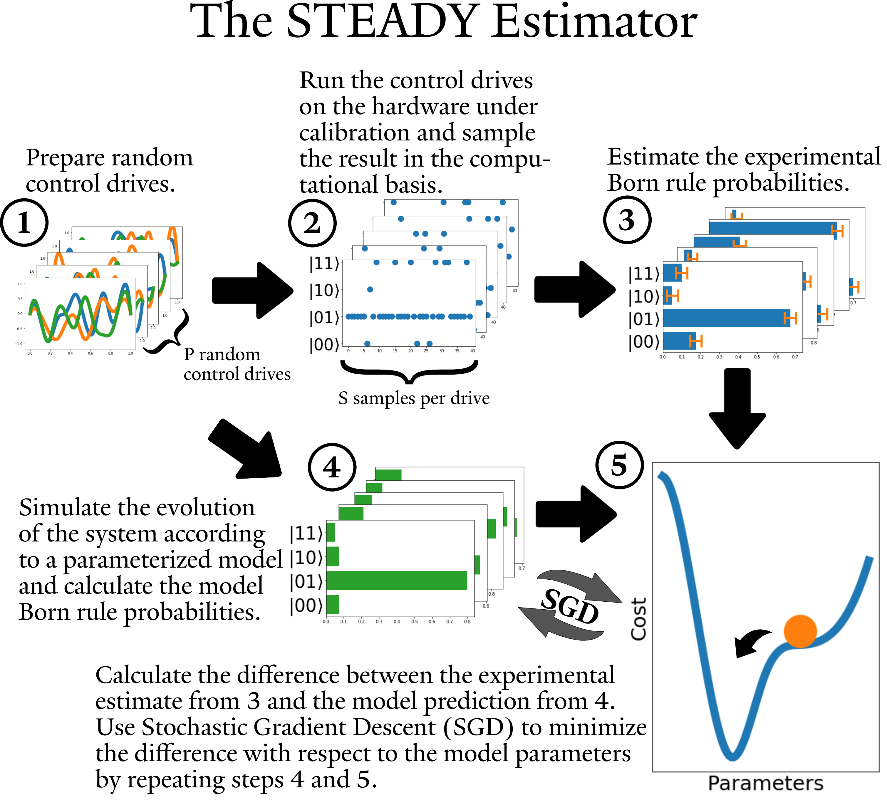
Here we present STEADY, a conceptually simple but performant method for approaching the parameter estimation problem for dynamical variables. We can model a piece of quantum hardware with a Hamiltonian (or Lindbladian) which depends on the parameters to be estimated and on the control pulses . Our goal becomes finding the value for that leads to an that (for any value of the control pulses ) most closely mimics the dynamical law governing the real hardware. As is commonly done in parameter estimation, we do this by searching for a value of that minimizes some measure of distance between and .
Our contribution follows in the rich traditions of stochastic methods and compressed sensing: instead of performing full process tomography on the hardware which would be extremely time consuming, we run a relatively small number of random control pulses on it and study its response. For each control pulse we sample the final state of the system (for instance by projectively measuring the qubits in the computational basis). We then estimate the difference between this experimental measurement and the prediction based on the model. This measure of “difference” is stochastic, as it uses only a small finite sample of possible control drives.
This leads to a number of properties that make STEADY perform particularly well. First, the distance measure that we use is differentiable with respect to which lets us use efficient (stochastic) gradient descent to rapidly find optimal values for the parameters being estimated. Moreover, the stochastic nature of our estimator leads to much lower resource requirements. We avoid doing full tomography, which greatly reduces the number of necessary measurements, while only modestly increasing the number of steps required by the (now stochastic) gradient descent. Simultaneously, the stochasticity lets us surpass the error floor otherwise imposed by the finite number of measurements performed when sampling the final states of the system. By using pulse sequences of varying lengths, our method becomes inherently insensitive to state preparation and measurement (SPAM) errors. The fact that dynamical variables—Hamiltonians and Lindbladians—are local quantities means that our estimates are generally sparse descriptions of the noise in a system, in contrast to an estimate that reconstructs a finite-time evolution of the noise. This allows regularized estimators to be used that avoid overfitting and lead to good estimates with surprisingly few data. In fact, our estimator can be restated as a maximum likelihood estimator which naturally approaches the information-theoretic limit of the Cramér-Rao bound.
Background
In the field of quantum computing there is a long history of achievements in both parameter estimation and control theory: the design of precise control schemes Peirce et al. (1988); Dawson and Nielsen (2005); Krotov and Feldman (1983); Khaneja et al. (2005); Caneva et al. (2011) for the preparation of states Tannor and Rice (1985); Law and Eberly (1996), unitary operations Unanyan et al. (1998); Mischuck and Mølmer (2013); Heeres et al. (2015, 2017a); Krastanov et al. (2015), and even complete quantum channels Bacon et al. (2001); Shen et al. (2017) has permitted advances in metrology, chemistry, communication, and—more recently—quantum computation. These control schemes are, in return, informed by the precise description of the system, obtained through various tomographic measurements Leibfried et al. (1996); Chuang and Nielsen (1997); Poyatos et al. (1997).
One can simplify the control problem by considering only a discrete set of gates instead of studying the continuous control that a complete knowledge of the Hamiltonian would provide. As long as the available set of basic gates generates the unitary group, there is a known efficient compilation procedure Dawson and Nielsen (2005); Parent et al. (2017); Amy et al. (2017); Svore et al. (2017). The performance bottleneck is in estimating the exact behavior of the given gates. Techniques like process tomography Leibfried et al. (1996); Chuang and Nielsen (1997); Poyatos et al. (1997) have existed for a while, but they are susceptible to state preparation and measurement (SPAM) errors Merkel et al. (2013). Gate set tomography Merkel et al. (2013); Blume-Kohout et al. (2013); Greenbaum (2015) mostly circumvents issues of SPAM, by requiring the preparation of only one type of state (e.g. the ground state) and only one type of measurement (e.g. in the computational basis). However gate set tomography is still susceptible to what Greenbaum (2015) calls “intrinsic SPAM errors”: state preparation errors for the ground state (e.g. a finite temperature of the system) and any imperfections in the projective measurement in the computational basis. Finally, there are tools like randomized benchmarking Emerson et al. (2005); Knill et al. (2008) that quantify average error rates of quantum processes (instead of the entire channel) without SPAM, and so can be used only as a benchmark, not as a tool for direct calibration (though extensions of the idea do allow this Kimmel et al. (2014)).
On the other end of the spectrum are control schemes that compute new control pulses for every single unitary operation (instead of compiling them out of the predetermined “universal” set of gates). This type of “continuous” control provides for quantum circuits with an order of magnitude smaller depth Heeres et al. (2017b); Boixo et al. (2018); Neill et al. (2018), however, it is also computationally more difficult. A popular approach to it is the use of gradient-based methods like GRAPE Khaneja et al. (2005). The fidelity of a given operation (the difference between the desired operation and the operation actually implemented by the control pulse) is computed as a function of the control pulse parameters. The fidelity is a differentiable function and its gradient with respect to the control pulse parameters is also computed, thus permitting efficient gradient descent, leading to a locally optimal control pulse. A large body of work is available discussing how to avoid getting stuck in local optima Brif et al. (2010); Zahedinejad et al. (2015); Palittapongarnpim et al. (2016). Recent development in the use of reinforcement learning has even provided for gradient-free techniques robust to noise Chen et al. (2014); Bukov et al. (2017); Niu et al. (2018).
However, most of the gradient-based control techniques require precise knowledge of the Hamiltonian in order to provide high-fidelity control drives. Some adaptive techniques get around this problem by switching to an in-situ method when they are near the optimal pulse. When the imprecisions in the model Hamiltonian start dominating, they forsake the model and start measuring the pulse fidelity experimentally through process tomography Egger and Wilhelm (2014); Wu et al. (2018) or randomized benchmarking Kelly et al. (2014). However, this makes the optimization much less rapid as the gradient is not directly available anymore and techniques like downhill simplex become necessary. Such optimization techniques are limited by the statistical error in the fidelity estimation. Recently, an elegant workaround based on “simultaneous perturbation stochastic approximation” was suggested in the ACRONYM method Ferrie and Moussa (2015), breaking through this statistical error floor. Impressive improvements have been seen in experiments following variations of these methods Rol et al. (2017). In either case, however, many additional experimental samples are required, but are then discarded after the current iteration of the optimizer. Moreover, all of these additional measurements are done for the sake of designing one specific gate with exquisite precision, but they do not contribute to estimating the Hamiltonian of the system and are forsaken when later on one tries to design another gate.
Here we focus on the precise estimation of the Hamiltonian itself, which can later be used in any control scheme. We suggest STEADY, a simple, but powerful approach that exploits the entirety of the measurement data in the Hamiltonian estimation, reaching the fidelity limits imposed by information theory. Similarly to ACRONYM, we use stochastic techniques to surpass the statistical error floor. Similarly to gate set tomography we are inherently insensitive to SPAM errors. Moreover, borrowing ideas from randomized benchmarking, our method can circumvent even the intrinsic SPAM errors (like finite temperature in the preparation of the ground state). The random pulses, informationally incomplete measurements, sparse models, and regularized estimators that we use take advantage of compressed sensing methods for state and process tomography Gross et al. (2010); Flammia et al. (2012) to improve accuracy. Lastly, STEADY estimates the complete Hamiltonian or Lindbladian (or other dynamical models, e.g. a stochastic master equation) of a system, not just one gate or a set of gates.
A recent independent preprint (Flurin et al., 2018) by Flurin et al. presents techniques similar to STEADY’s with significant differences in the design choices. While the prescription for gathering experimental data and the comparison of the model to that data are very similar in both approaches, Flurin et al. use a recurrent neural net (RNN) to model the dynamics, while we use physical models with very general parametrization. Flurin’s black box approach is promising for models that are particularly difficult to differentiate, like stochastic master equations, however modern autodifferentiation frameworks (Innes, 2018) enable the use of STEADY as well. Furthermore, the RNN size is expected to grow exponentially with the number of qubits in order to simulate the quantum dynamics. That exponential cost is explicitly present in STEADY. It would be interesting to examine whether the RRN, after hyperparameter optimization, would find a sparse representation of the dynamics, similarly to STEADY’s use of Hamiltonian and Lindbladian generators which are explicitly a sparser representation of the otherwise dense superoperator.
In the following we specify the formalism we use to describe the protocol and demonstrate that it reaches the information theoretical limit in estimation fidelity. We discuss the effect of the intrinsic SPAM errors and how to circumvent them. Experimental design techniques that further improve the fidelity of our estimator are described. We briefly discuss the effects of parameter drift, non unitary errors, and nonlinearities in the Hamiltonian (as a function of the control pulses). Together with this manuscript we also provide a software package based on a popular differentiable programming framework Abadi et al. (2015) that implements our techniques for various models including unitary or non-unitary evolution.
Problem statement
A system of qubits (a -dimensional Hilbert space) is controlled by a Hamiltonian (that is itself a function of time-dependent control pulse set by the experimentalist). is a -dimensional real vector, where is the number of control parameters available to the experimentalist. The evolution of an initial state will then be expressed as
| (1) |
To accurately predict this dynamics we must learn the Hamiltonian as a map in order to be able to control the quantum hardware using a control pulse . We introduce a parameterized model for the Hamiltonian, , in which case the problem becomes finding the values of all parameters in the array for which for all . We will also discuss the case where the model cannot exactly represent the reality of , as well as cases where non-unitary evolution is non-negligible.
With some a priori knowledge of the physical system, an experimentalist might be able to deduce an approximation of , however the experimentalist could also run experiments on the hardware to learn successively better approximations of . An experimentalist can run a control pulse and then project and measure the final state of the system in the computational basis. The details of how the pulses are chosen and how the measurement data is used distinguishes the various approaches to Hamiltonian estimation and calibration like process tomography Leibfried et al. (1996); Poyatos et al. (1997); Chuang and Nielsen (1997), gate set tomography Blume-Kohout et al. (2013); Greenbaum (2015), and randomized benchmarking Emerson et al. (2005); Knill et al. (2008); Kimmel et al. (2014).
Unlike most estimation techniques, we work at the level of control pulses, without hiding them behind a set of precompiled gates. Moreover, our protocol is inherently untroubled by SPAM errors, as no special states or measurements are necessary, besides preparing the ground state and performing measurements in the computational basis, just like in gate set tomography. We improve even further by partially circumventing the intrinsic SPAM errors found in gate set tomography Greenbaum (2015).
Methods
To describe our protocol, we will first consider only Hamiltonians that are linear in the control pulse. This is an appropriate description when some prior knowledge of the relationship between the control fields and the Hamiltonian is known, but more general mappings could be addressed as well, as we discuss below. The model for such a Hamiltonian in its most general form would be (in index notation for )
| (2) |
where and belong to arrays of complex numbers representing the parameters that need to be learned. The numbers form the elements of a matrix and can be interpreted as the drift Hamiltonian of the system, and the numbers (forming a array) can be interpreted as the list of control Hamiltonians (one for each control parameter in , where could be time dependent). Hermiticity can be ensured if the parametrization is done in terms of pairs symmetric and antisymmetric real matrices. There are real parameters to be learned in this case.
Such a high level of parametrization might be unnecessary for a well studied system. In such a case one can list the fixed known Hermitian operators that are part of the Hamiltonian in a large list (where we have such possible operators) and only parameterize how these operators are summed together in
| (3) |
Here and are arrays of real numbers representing the parameters that need to be learned. The -dimensional real vector represents all the drift components of the Hamiltonian, while the real matrix represents the linear mixing/crosstalk between drives. There are real parameters to be learned in this case. For the next few paragraphs we will consider only this low-degree-of-freedom parametrization, and later on we will discuss when one might want to use the more general approach. We stress that our approach is not limited to Hamiltonians linear in the control pulse parameters—any functional dependence can be used in place of the two discussed above. In particular, we discuss the estimation of a Lindbladian later in this manuscript, and even the measurement backaction parameters of a stochastic master equation can be studied using STEADY.
Experiments in this setup proceed by performing some form of regression on data that has been gathered from the hardware in order to find an approximation of . To gather the data we suggest the following approach. Begin by generating a large number of random control pulses on the classical computer controlling the hardware. For simplicity we will initially consider only constant pulses of fixed duration where each random pulse is taken from a normal distribution of unit variance centered on zero, but our approach is equally easy to apply to random time-dependent pulses sampled from other distributions with fixed variance. This provides us with a list of control pulses. Each control pulse is run on the hardware, initialized to the ground state, resulting in a final state
| (4) |
Experimentalists cannot exactly read the components of in a given basis (e.g. the computational basis), rather they can only estimate them through projective measurements. Specifically, our protocol requires the experimentalist to run each pulse times in order to repeatedly sample through projective measurements. For each (and corresponding ) this provides a vector of estimated Born rule probabilities . With an infinite number of samples , and the assumption that the unknown Hamiltonian parameters do not drift, the estimate would converge to be exactly the Born rule probability vector (the -th component of is , where enumerates the computational basis). Similarly, the Born rule probability for a given drive predicted by the model Hamiltonian will be denoted (its -th component is ). We note that when the model contains the true Hamiltonian then .
We can define the “distance” between the measured estimate for the population and the predicted population, averaged over the random pulses:
| (5) |
Our estimator for is the minimum of this distance measure (called the “cost function” from here on):
| (6) |
If the distance function is the cross entropy, i.e. , then our estimator is a maximum-likelihood estimator. For most of the numerical examples, the distance function we use is the mean squared error , which is simpler, but in practice leads to the same estimate. The cost function is differentiable, which permits us to run automated stochastic gradient descent optimizers in the search for . In practice, we also augment this cost function with a regularization cost for to avoid overfitting and enhance convergence, as discussed in the supplement. Ideally, we would have the sum run over all possible control pulses, but this is unfeasible in finite time. Stochastic gradient descent, where only a small number of random pulses is used, is what enables our method thanks to its strong guarantees of convergence to the same minimum.
Results
In the next few paragraphs we study the performance of this method. In order to check our susceptibility to over-fitting or convergence failures, we also introduce a validation cost function (which would be unavailable to the experimentalist, but is available on our simulated “mock” hardware)
| (7) |
where is the size of , a new set of random “validation” control pulses sampled from a unit-variance distribution. This validation function does not suffer from the statistical noise inherent to finite : it is a sample estimate of the cost function over pulses, and it is the expected value over measurements. Moreover is non-negative and , hence , given our choice of distance function (see supplementary materials). We will keep the validation set the same in all comparisons, even if we change the size, variance, or anything else related to the training set . Similarly, for the validation function we always use a pulse of unit duration, even if we decide to use different duration pulses for the cost function.
The validation function is defined so that small values of imply good predictive power of the empirically reconstructed model. Our validation function was chosen for this reason and for its close connection to the cost function, but in the supplementary materials we demonstrate that other more common measures of fidelity have the same scaling.
For most of this manuscript the distance function in and is the mean squared error and other choices are discussed in the appendix. Unless specified otherwise, numerical results are given for , and a simulated system of qubits, driven by Pauli drives and nearest neighbor exchange interactions, where gives the relative strengths of each drive. Details are provided in the supplementary materials.
Statistical Sampling Errors

If we could obtain a perfect estimate of the populations (i.e. if we could have ), then even a small data set (a small ) would be sufficient to perfectly estimate the Hamiltonian parameters. The only issue would be ensuring our system is not under-constrained by having , and regularizing the gradient descent procedure to ensure we are not stuck in a valley of the cost function. Indeed, when , we rapidly converge to , a floor imposed by the floating point precision.
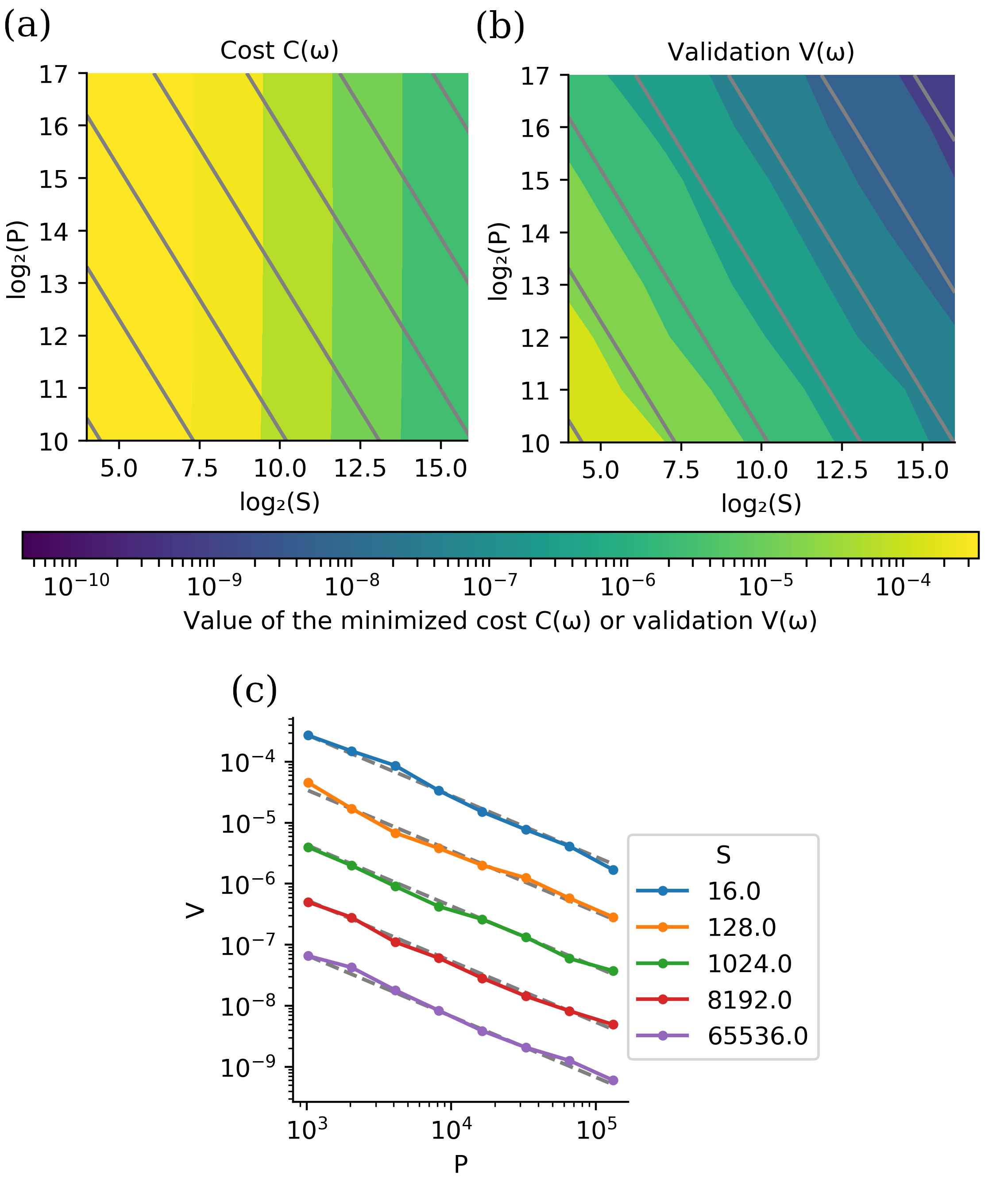
However, in a realistic case we could run the quantum hardware only a finite number of times , where a finite will incur a statistical error on . Given that obtaining is a multinomial sampling procedure from the distribution , we can expect an error , which would cause an error floor of . We would need to increase in order to get a better estimate of , as can be seen from the behavior of in Fig. 2a. From that figure one could think that increasing is important while increasing is a waste of resources, however, the minimized value of is a bad proxy of the quality of our parameter estimation given that it is inherently plagued by the statistical error. This is why we have introduced the validation function , which in Fig. 2b. shows that the total amount of information is the important resource expended in parameter estimation. The precision of our estimate scales as , i.e. inversely with the total amount of measurements we take from the hardware. It is inconsequential how we group the data (more pulses or better estimation of the result from fewer pulses) as long as is kept constant and is sufficiently large to constrain the system. In fact, as long as we have good regularization that ensures convergence of the gradient descent procedure, even (where becomes a binary vector) performs just as well.
On first sight it can be counter intuitive that the validation function continues to improve even when the actual cost function reaches a floor, but this is similar to the difference between the standard deviation of a distribution (taking the role of ) and the possibly much lower standard error in the estimator of the mean of that distribution (taking the role of ). Such behavior is typical of stochastic optimizers and can be seen in ACRONYM Ferrie and Moussa (2015) as well. A linearized example of this can be seen in the supplementary material. A more rigorous understanding of this effect can be presented in terms of the Cramér–Rao bound Cramér (2016). The variance of each component of our estimator for is bounded by , where is the corresponding component of the diagonal of the Fisher information matrix for our measurements (without loss of generality, we assume the parameter vector is chosen so that no two distinct components have nonzero correlation). Moreover, , where is the Fisher information for the estimator of a single projective measurement for a given pulse and denotes an average over all control pulses . The projective measurement is equivalent to sampling once the multinomial distribution described by , hence , where . For the purposes of statistical errors we can already observe that for every component of we have
| (8) |
This confirms our observations from Fig. 2, and proves the efficiency and unbiasedness of our estimator.
Intrinsic State Preparation and Measurement Errors
The discussion from the preceding paragraphs did not consider the effects of imperfect state preparation and measurements (SPAM). Unlike with process tomography, we do not need to prepare initial states spanning the whole Hilbert space, nor do we need to make projections in anything but the computational basis. As such, STEADY is not susceptible to the usual SPAM errors, an advantage we share with gate set tomography. However, both gate set tomography and STEADY suffer if the ground state is not properly cooled or if the measurement in the computational basis is not perfect (effects called “intrinsic SPAM” by Greenbaum (2015)). Below we study the error floor caused by the intrinsic SPAM and describe how our protocol is able to deal with it. Our model for intrinsic SPAM in the numerical examples is parameterized by a single parameter , which is defined as the probability that any given qubit might have flipped from to during state preparation. We also choose the probability that a projective measurement is incorrectly reported as its opposite to be this same value . For numerical simplicity second order effects are neglected, i.e. two qubits cannot flip at the same time (during preparation or measurement). The detailed exact expression for the intrinsic SPAM model we use is also given in the supplementary materials.
As one can see from Fig. 3(b), increasing the intrinsic SPAM probability (the per-qubit error rate for initial state preparation or final projective measurement) leads to a breakdown of the scaling and an intrinsic error floor that cannot be surpassed by simply increasing the available data. The Cramér-Rao bound is not immediately useful in explaining this effect, because we have initially phrased it in terms of an unbiased estimator for . However, the intrinsic SPAM errors contribute to a bias in our estimator, in which case the bound becomes
| (9) |
where is an expectation value over all possible sets of measurements, and is the bias of the estimator of .
In Fig. 3(d) we see the appearance of an error floor in the fidelity/validation function. We observe , which unsurprisingly points to a bias that grows with the intrinsic SPAM error (behavior that can be observed by leading order expansions of the validation function, as done in the supplementary materials).
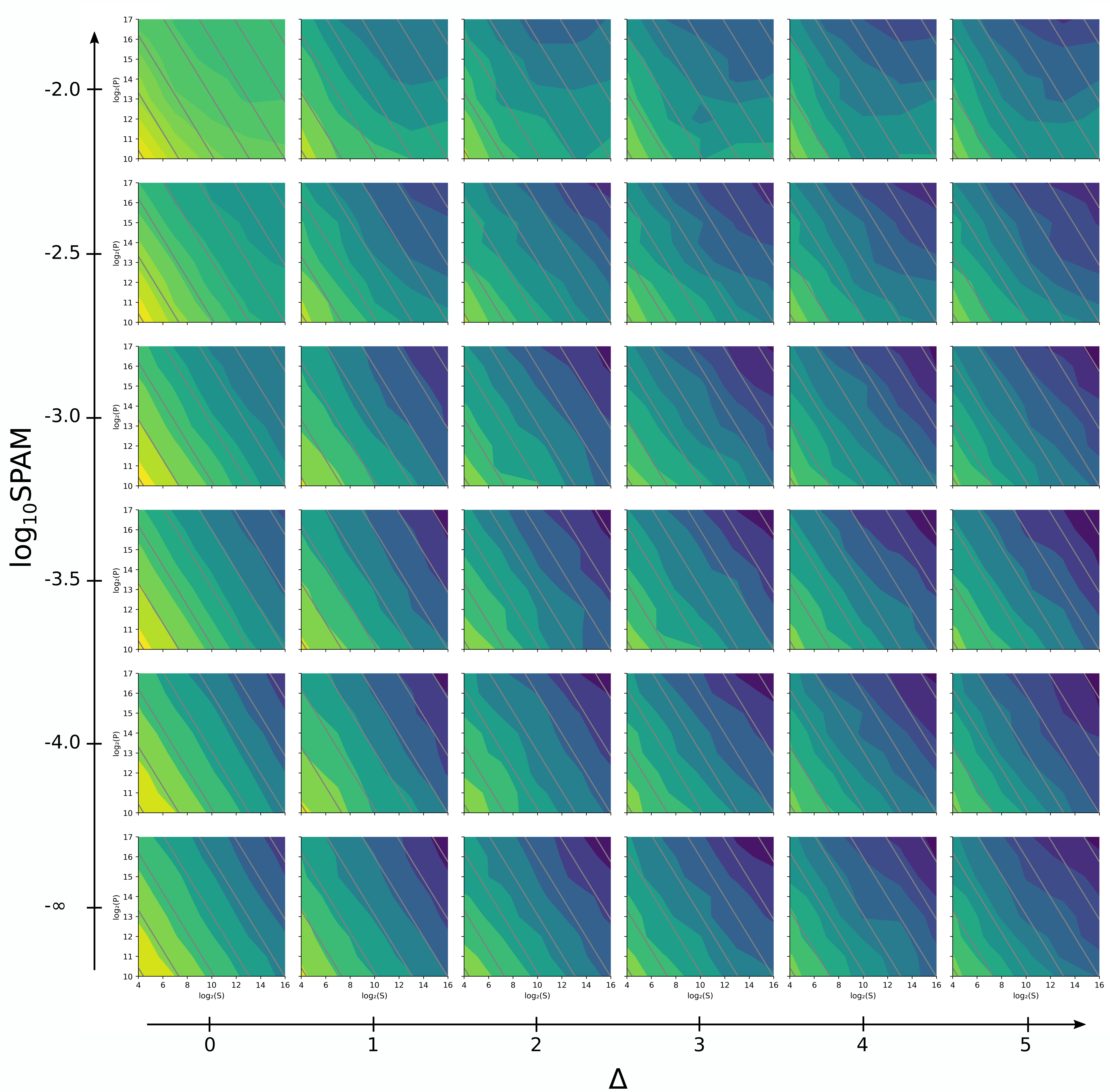
An inspiration from randomized benchmarking leads to a way to surpass this error floor, namely that longer control pulses would suffer from fixed SPAM errors, but greater and greater coherent bias-induced errors. Anywhere that appears, it is multiplied by , leading to . Doing the same Taylor expansion as described above leads us to . We do observe in Fig. 3(c) that we rapidly return to the much lower statistical error by using longer pulses. Equivalently, instead of using longer pulses, we can use pulses of greater average power. Thanks to this, STEADY provides for addressing not only statistical errors (by taking more samples), but also intrinsic SPAM errors (by using longer/stronger pulses).
A figure with a more exhaustive numerical report over various pulse lengths and SPAM error rates is presented in the supplementary materials.
Another way to fight the effects of SPAM is to include them in the model of the dynamics, and estimate the parameters governing SPAM together with the unitary parameters. Later in the manuscript we discuss such approaches of extending the model to describe more general dynamics like non-linear drives and non-unitary effects.
Optimal Control and Experimental Design
The usual goal of estimating the parameters describing one’s hardware would be to permit high-fidelity open-loop control. There is a rich history of methods designed for that purpose Law and Eberly (1996); Mischuck and Mølmer (2013); Krastanov et al. (2015); Heeres et al. (2017a); Leung et al. (2017); Mavadia et al. (2017). Lately, optimal control techniques have been used with great success. The “differentiable programming” toolkits Abadi et al. (2015) that have enabled the rapid development of STEADY is readily applicable to the reverse problem of optimal control Leung et al. (2017): we “freeze” the model parameters and now optimize with respect to the control drives, while the minimization target is not the distance between a measured and predicted state, but rather between the desired and predicted state.
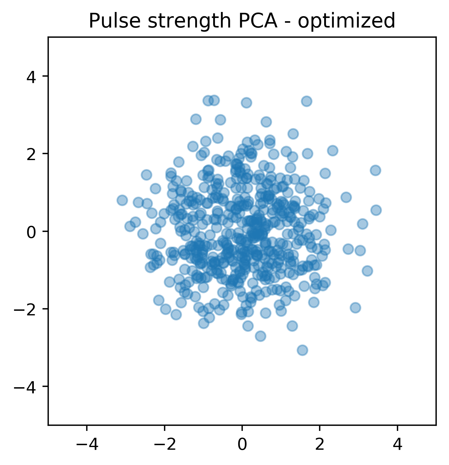
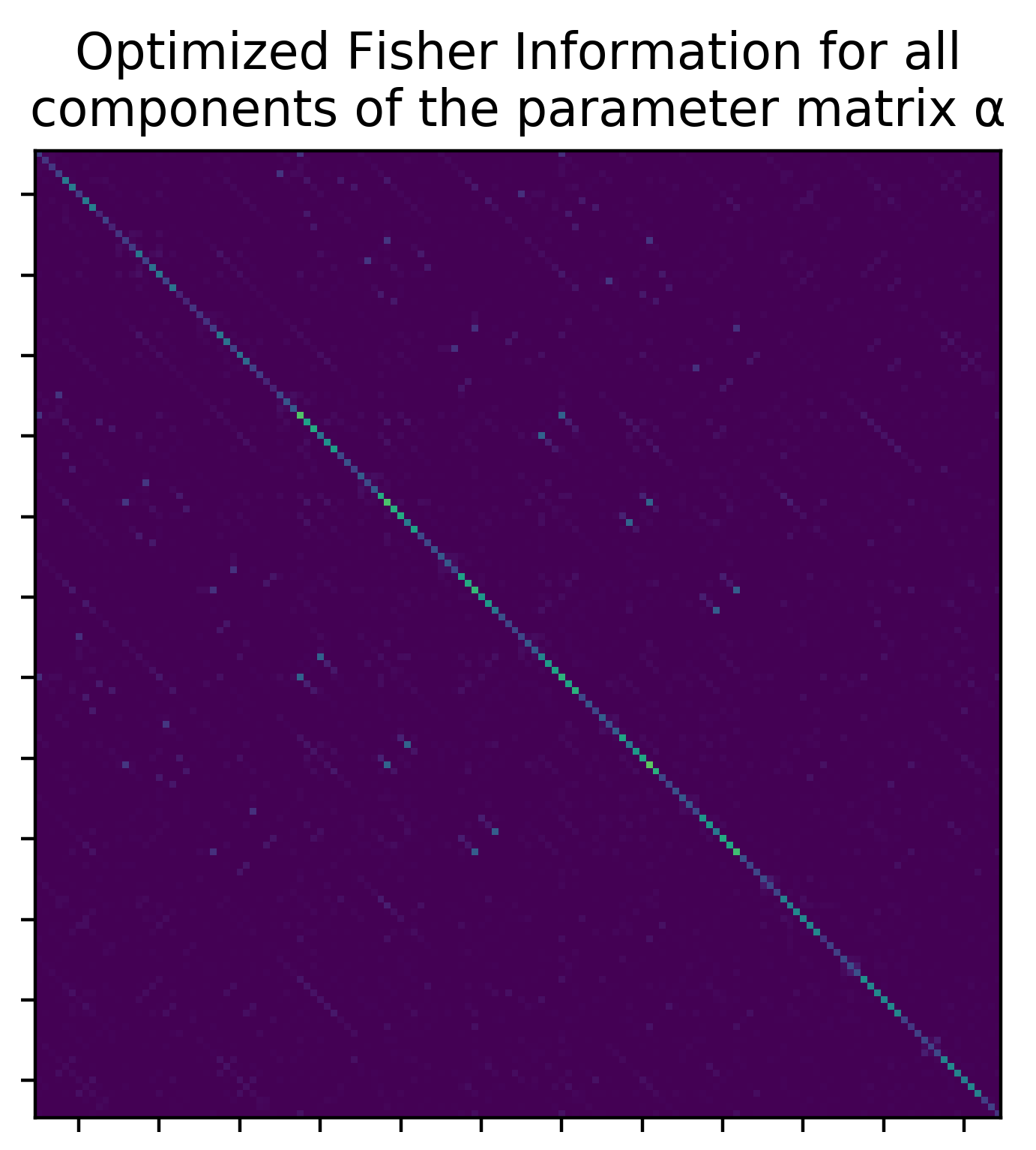
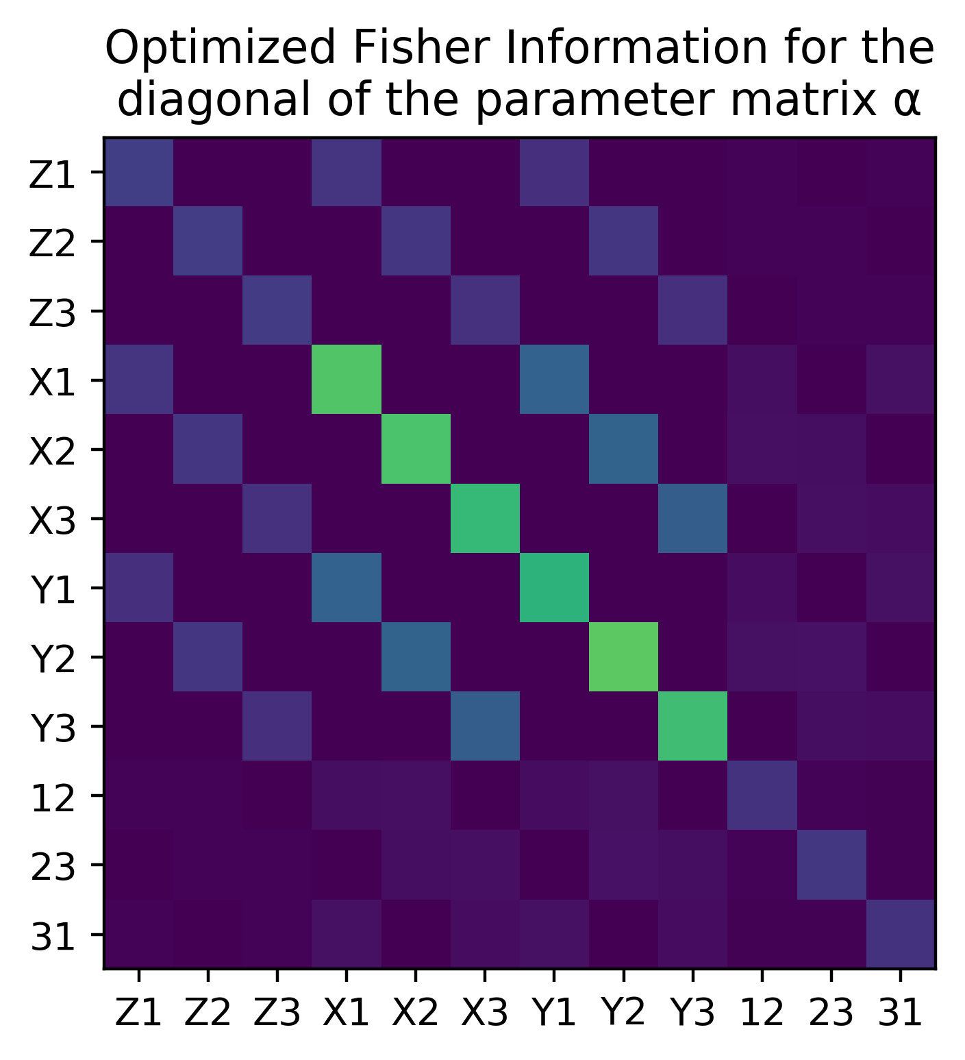
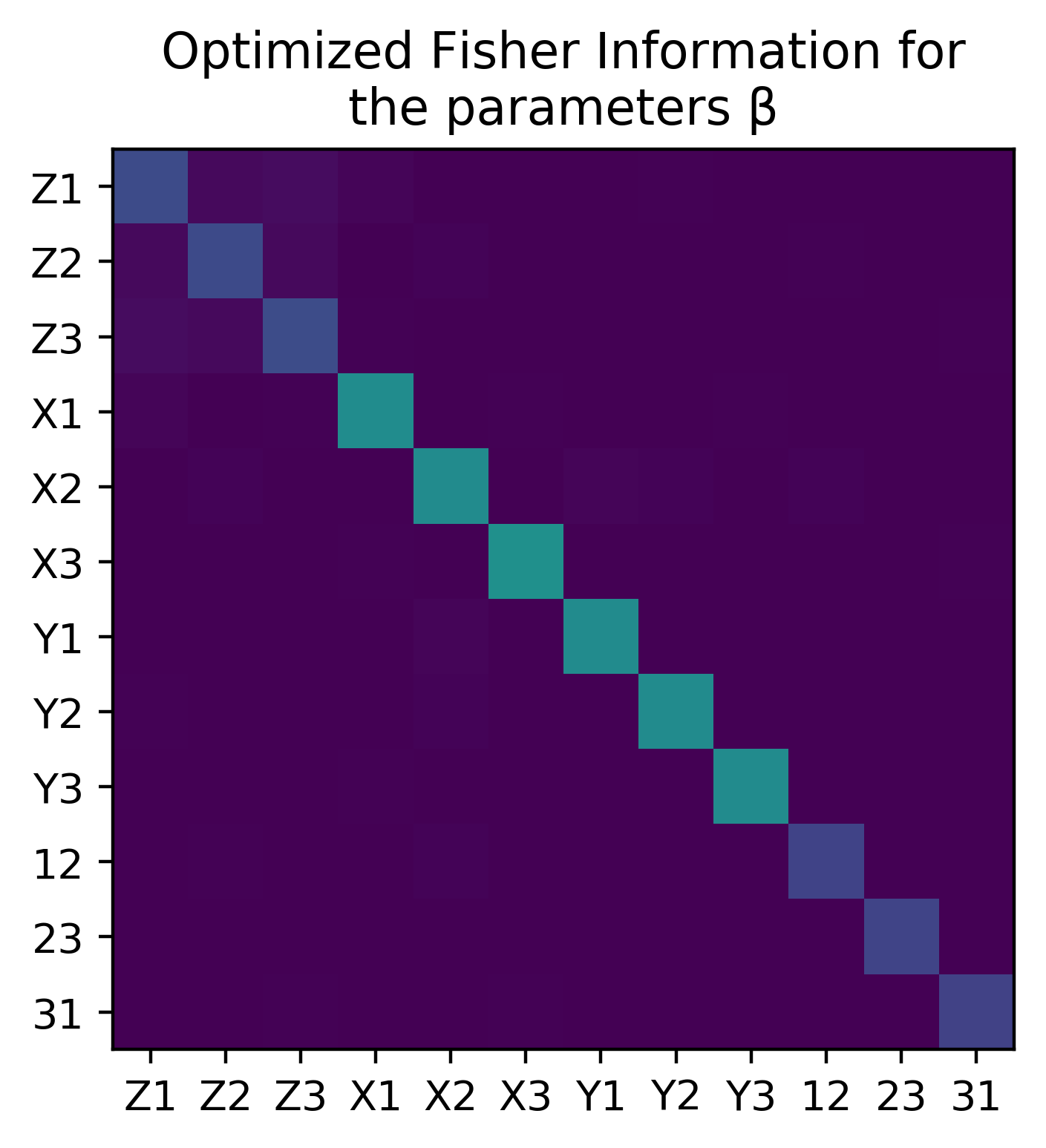
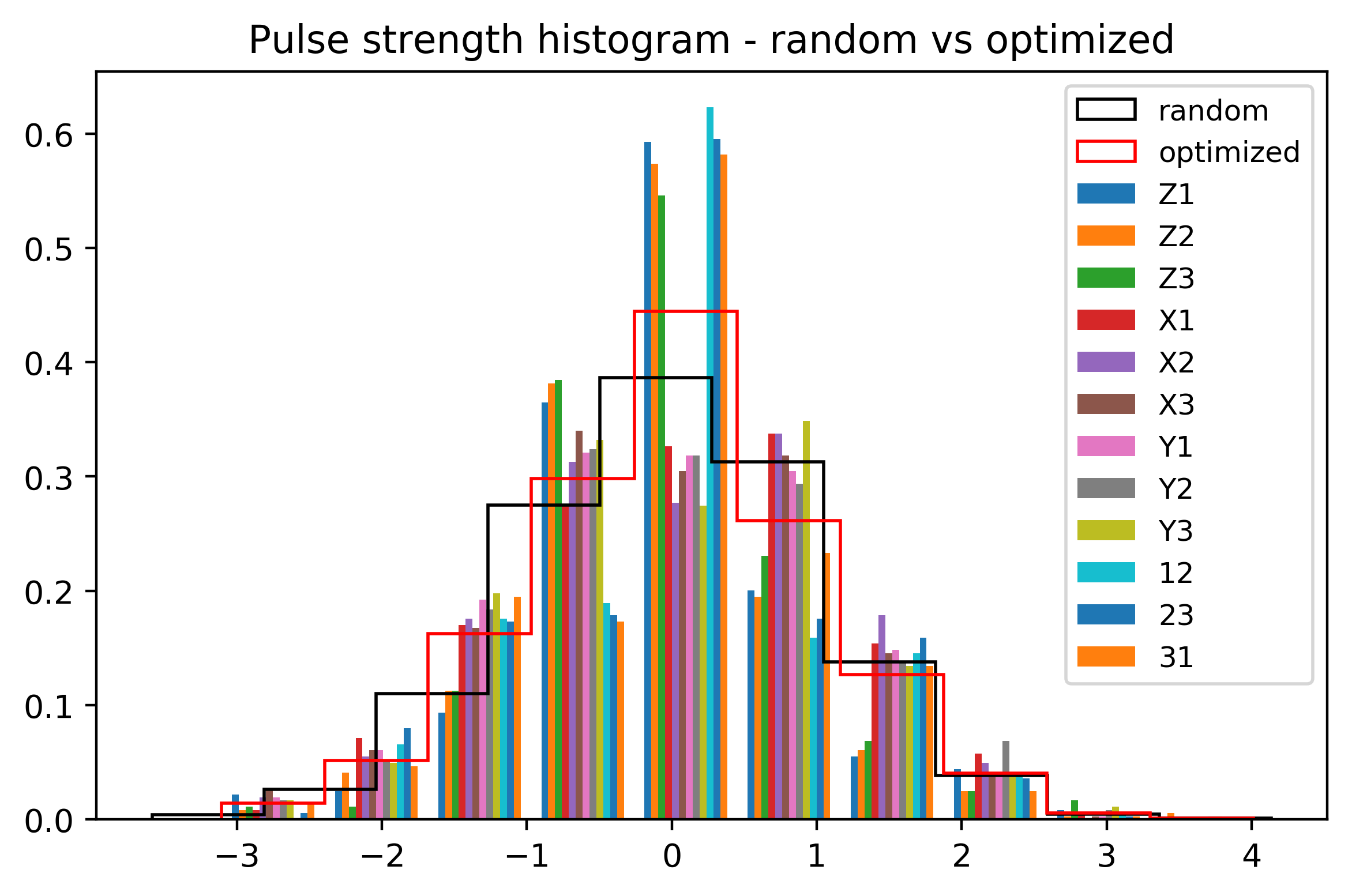
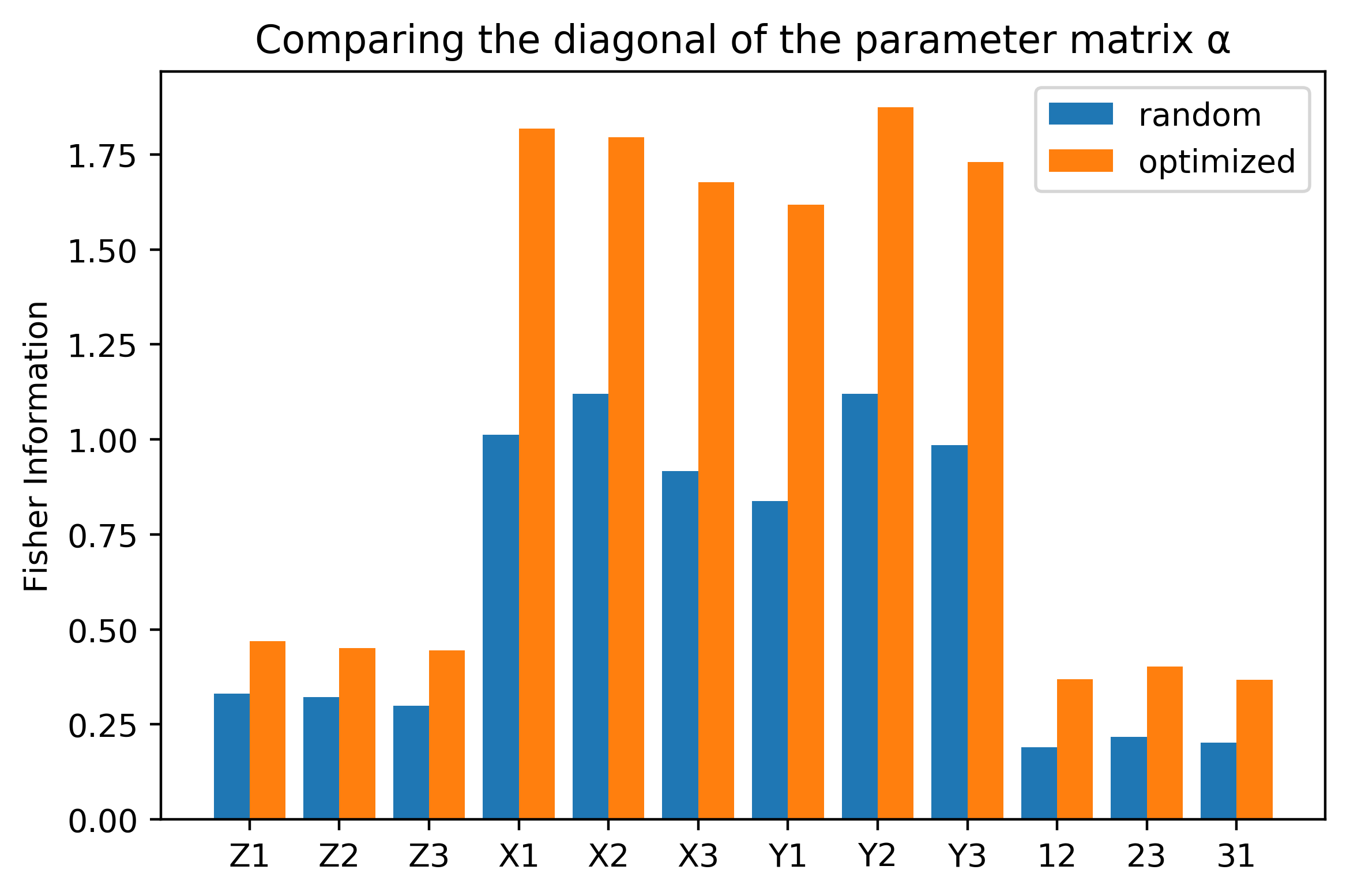
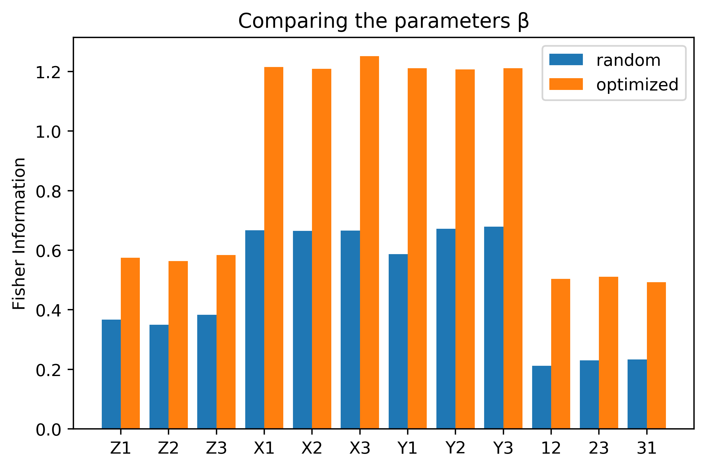
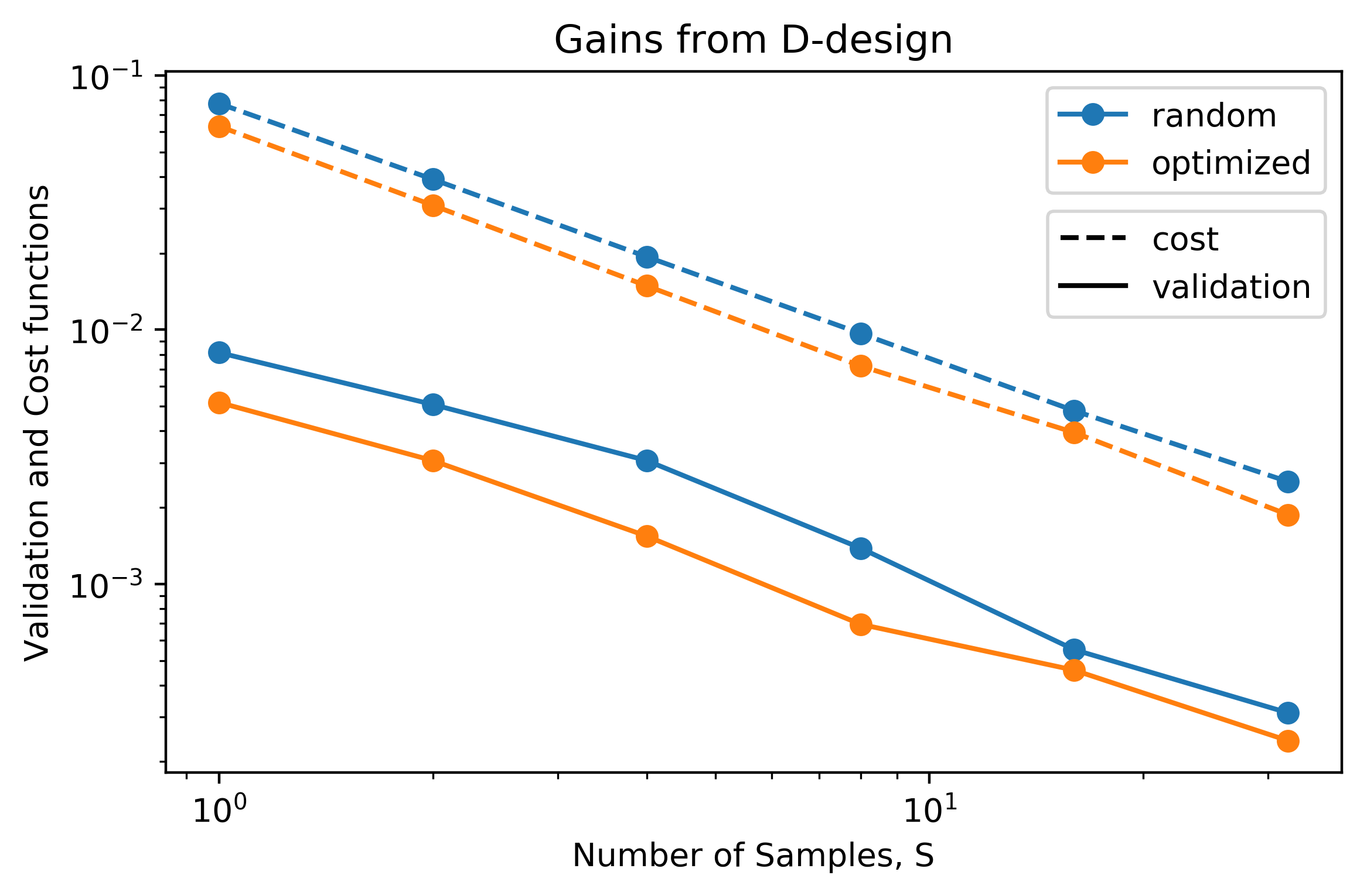
However, in the context of our work, there is a more exciting application of optimal control, that would permit parameter estimation at much lower resource/time cost. As we have described in previous sections, the fidelity of any estimator is limited by the Fisher information contained in our measurements. Here we suggest a relatively straightforward optimization procedure to increase the available Fisher information. This procedure will perform well in practice, and as we have shown, it continues to saturate the scaling behavior of the Cramér–Rao Bound, but it is not globally optimal. As our task is a multiparameter estimation problem and parameters that couple to noncommuting observables cannot be measured simultaneously without disturbance, the optimal estimation scheme is unlikely to be as simple as the use of random control pulses in STEADY (we refer the reader to Refs. (Pezzè et al., 2017; Matsumoto, 2002; Yang et al., 2018) for an overview of the literature on optimal multiparameter estimation). Instead of using random control pulses we can also run gradient descent to find the control pulses that maximize the determinant of the Fisher information of the measurements (also known as D-optimal design in the field of experimental design). This optimization procedure does not need to converge with great precision to the true maximum, as we are interested in the gross gain obtained from switching from random pulses to optimized pulses (the minor gain from precisely finding the maximum is negligible in this context). Fig 4 demonstrates how STEADY can halve the required number of measurements while obtaining the same fidelity, thanks to this careful design of control pulses. We have kept the average power of the control pulses fixed to a single unit, both in the case of random and optimized pulses. In our mock tests this technique has been able to provide similar gains in the fidelity of the estimator over a large range of values for or .
Discussion
There are a number of technical details and caveats that need to be addressed.
First, the stochastic gradient descent could have trouble reaching the optimum due to difficult-to-traverse valleys in the cost landscape. In practice, annealing the learning rate in an adaptive Nesterov-momentum Adam optimizer Nesterov (1983); Kingma and Ba (2014), together with annealing of a 1-norm regularizer (following MacKay’s “empirical Bayes” trick MacKay (1992)) was sufficient for robust performance of our estimator. These choices were informed by a hyper-parameter optimization study. We provide more details about this in the supplement.
Many hardware systems could be plagued by slow drifts in the Hamiltonian. Approaches to solving this issue span from estimating the drift (i.e. just making it one of the parameters describing the dynamics) to repeating the estimation procedure at regular intervals. Both techniques are readily applicable to our method, additionally opening the possibility to use efficient transfer learning Pratt (1993) if necessary.
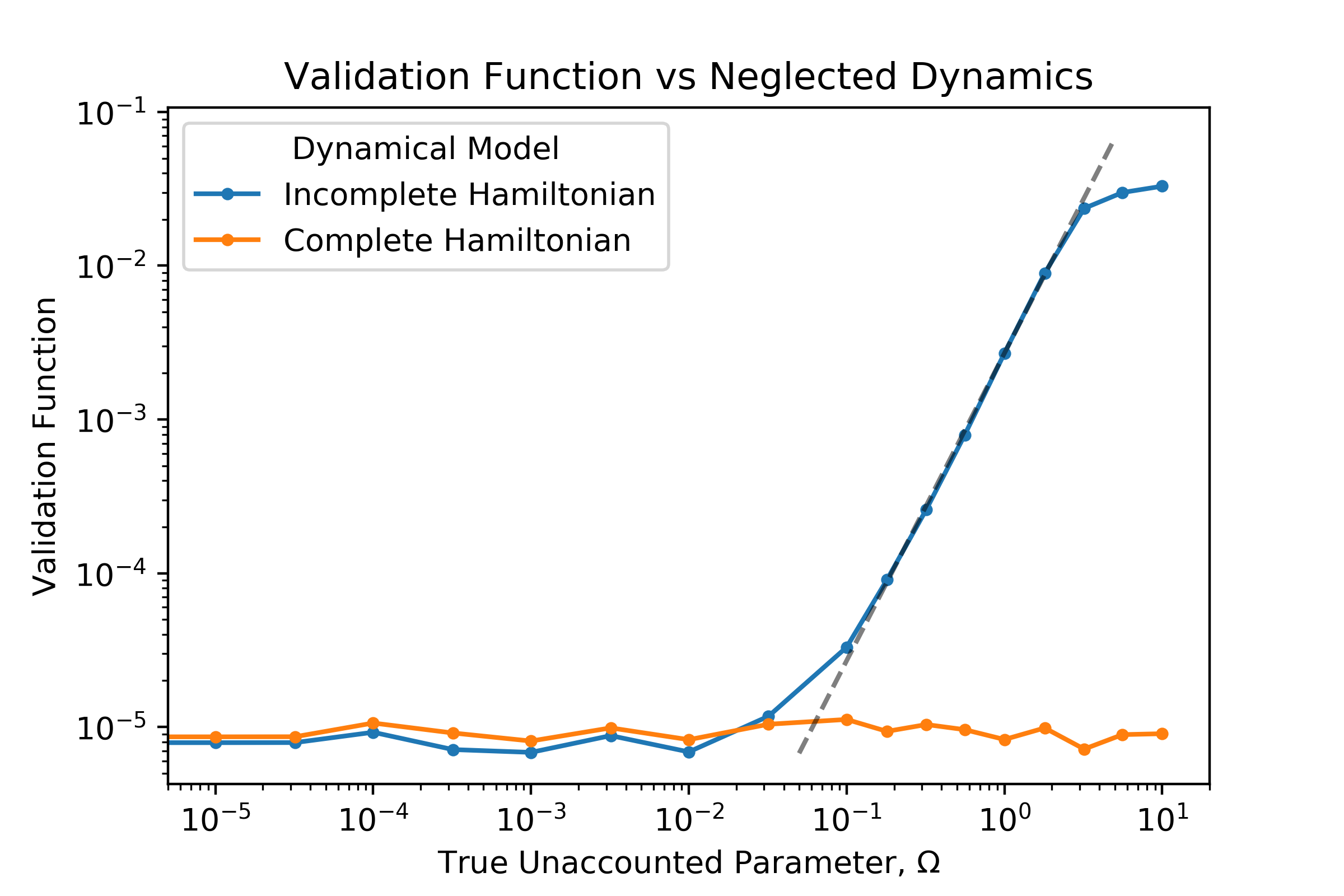
It is important to also note that our approach for circumventing the intrinsic SPAM errors assumes that our model is capable of exactly describing the actual dynamics of the system. There are two cases in which this might not be true. On one hand, we might have coherent errors, due to small corrections to that are not described by the map . Such problems can be straightforwardly addressed by parameterizations of that include quadratic and higher terms.
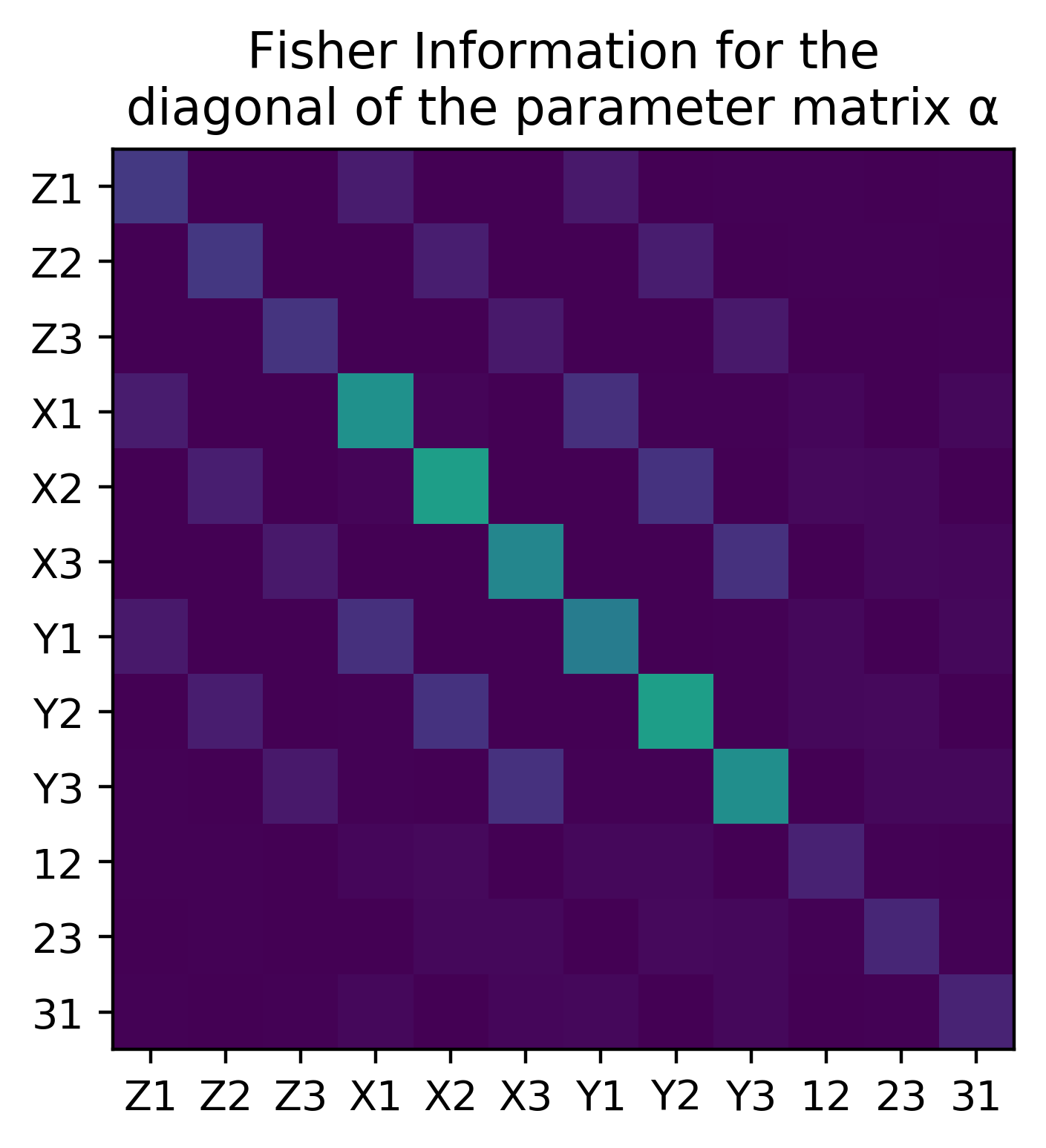
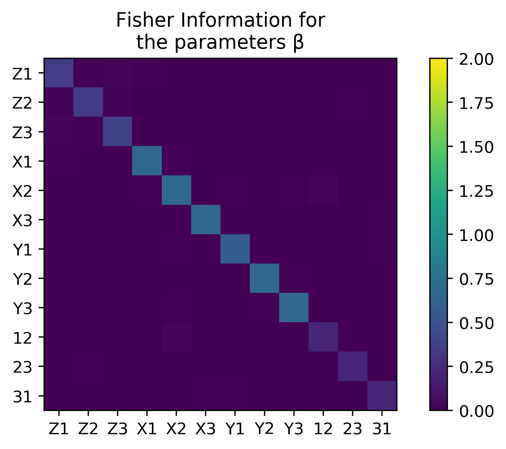
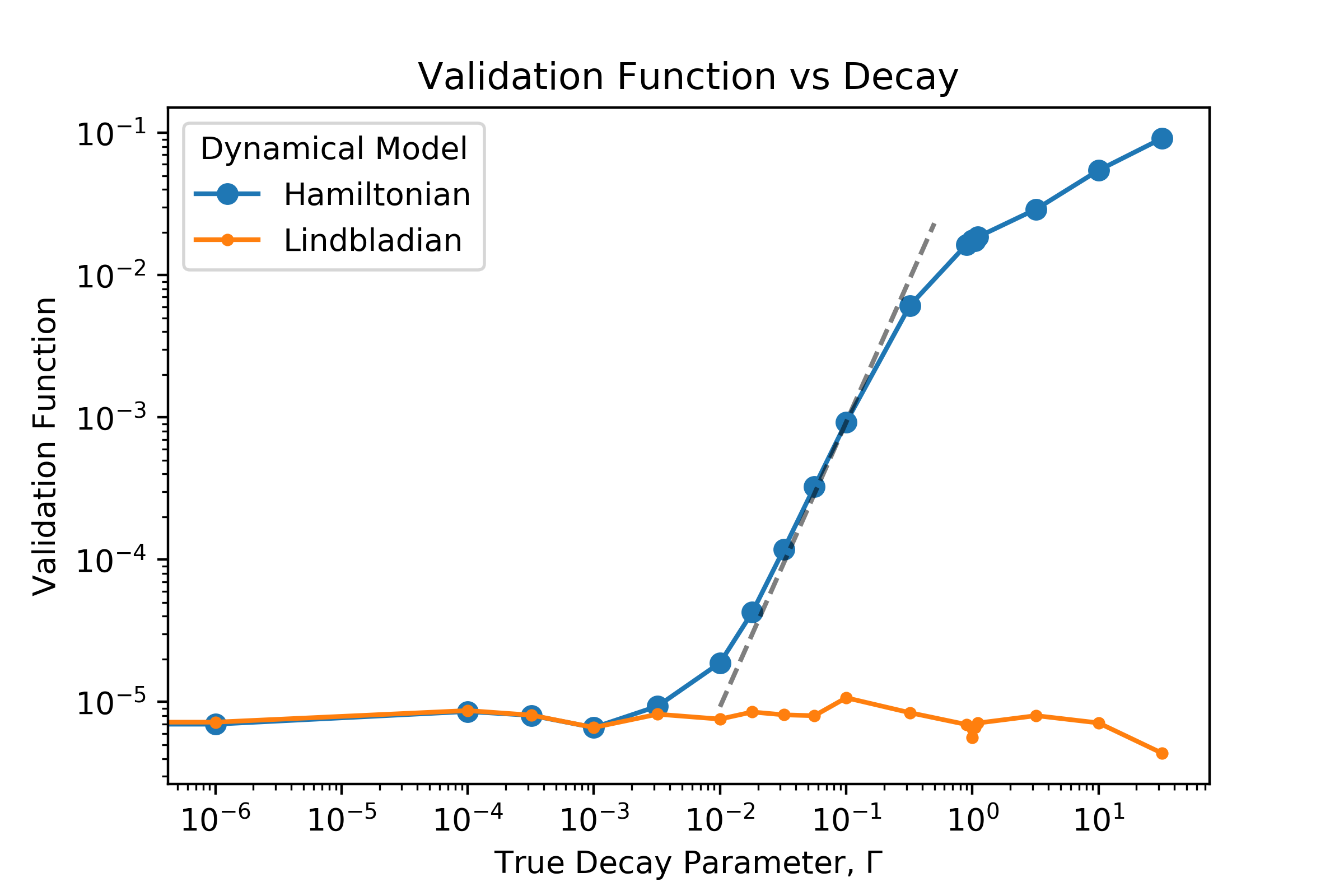
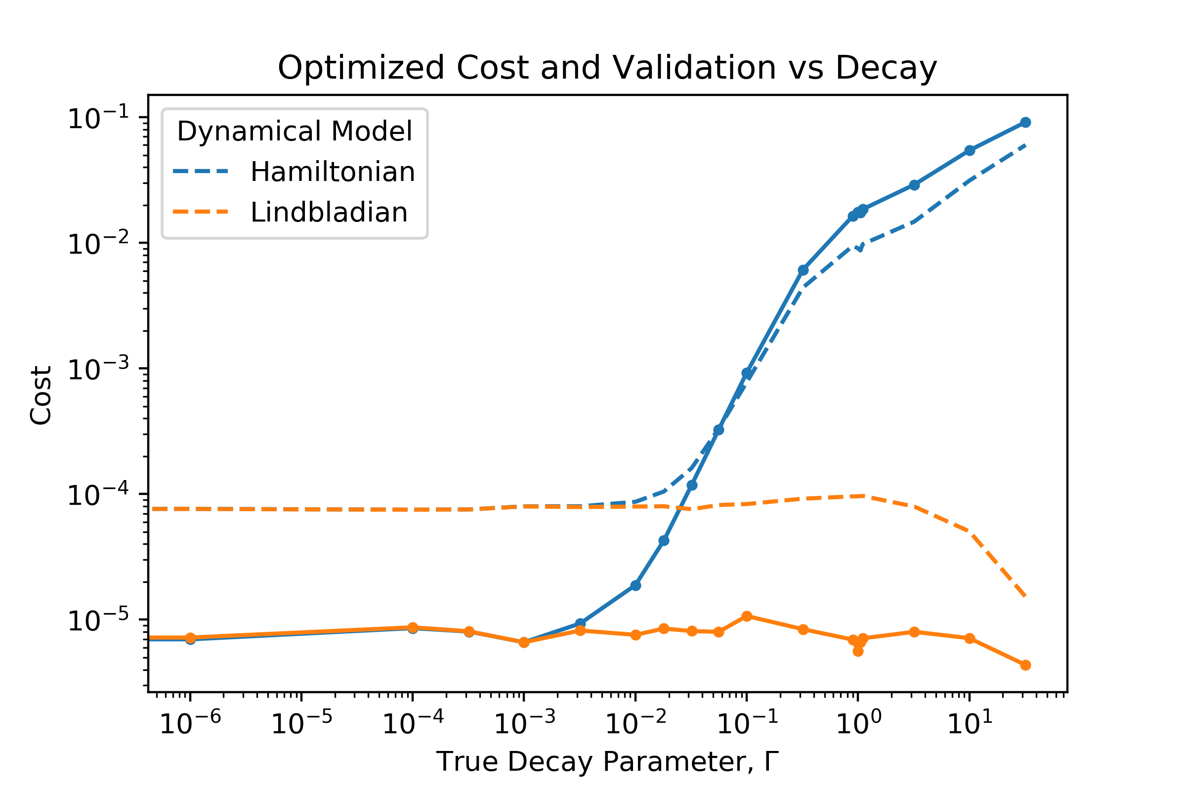
A special type of error that can never be captured by the Hamiltonian formulation above would be an inherently non-unitary error such as decay or dephasing. The only way to fully capture the effects of such non-unitary dynamics is to include them in the model used by the estimator, and the most natural approach is to simulate the evolution of the system with a master equation. This leads naturally to the Lindbladian version of STEADY, which follows the same principles as the Hamiltonian version detailed above. Fig. 5 demonstrates that including the non-unitary dynamics in our model permits us to reach the statistical error floor that was unreachable with an incomplete Hamiltonian model. A more detailed discussion in terms of Fisher Information content for this Lindbladian case is provided in the appendix. Even more general dynamical laws can be implemented in STEADY as well: whether for use in classical mechanics, other dynamical systems, or in the rich field of continuous weak measurements of quantum systems (Flurin et al., 2018; Tsang, 2009; Cortez et al., 2017).
Conclusion
We have introduced STEADY, a method for Hamiltonian or Lindbladian estimation that reaches the information-theoretic performance limits. The method is inherently insensitive to general SPAM errors plaguing approaches like process tomography and can even circumvent the intrinsic SPAM errors (e.g. errors in the preparation of the ground state). Working at the Hamiltonian/Lindbladian level gives us greater control than what methods restricted to sets of pre-compiled gates provide, letting us use optimal control techniques when manipulating the system. This versatility permits us to use well known techniques like D-optimal experimental design to further improve the fidelity of our estimator.
There are many avenues that remain open for further exploration and extension. Because STEADY uses an inherently sparse description of the noise in the system, it is conceivable that the method could be made scalable. At the moment, this is precluded by the need to simulate the full quantum dynamics, but methods to speed this up could be employed such as using non-universal quantum circuits instead of random pulses, or using a well-calibrated quantum device together with STEADY to calibrate a new device. There is much room for additional theoretical work on the performance of STEADY, especially in regards to the family of models that we consider. Here we mainly considered a linear coupling to drives, but it should be possible to give a complete theoretical analysis of performance for more general classes of functions. It would also be interesting to include weak measurements in a stochastic master equation formalism and attempt to infer the measurement parameters as well. One additional open problem is to connect the performance of STEADY to other popular error metrics for quantum gates so as to facilitate an analysis of fault tolerant capabilities for quantum computation Kueng et al. (2016). Lastly, experimental implementation of these ideas will undoubtedly lead to further improvements in the method.
Acknowledgements.
This work would not have been possible without the contributions of the Python, Jupyter, Matplotlib, Numpy, Qutip, and Julia open source projects and the Yale HPC team. We acknowledge support from the ARL-CDQI (W911NF-15-2-0067, W911NF-18-2-0237), ARO (W911NF-18-1-0020, W911NF-18-1-0212), ARO MURI (W911NF-16-1-0349), AFOSR MURI (FA9550-14-1-0052, FA9550-15-1-0015), DOE (DE-SC0019406), NSF (EFMA-1640959), and the Packard Foundation (2013-39273). This work was also supported by the Australian Research Council through the Centre of Excellence in Engineered Quantum Systems CE170100009, and by the US Army Research Office grant numbers W911NF-14-1-0098 and W911NF-14-1-0103.SK performed the majority of the software development and numerical tests. The design, evaluation, and repeated iterative improvements of the method were jointly done between all four authors.
References
- Peirce et al. (1988) Anthony P Peirce, Mohammed A Dahleh, and Herschel Rabitz, “Optimal control of quantum-mechanical systems: Existence, numerical approximation, and applications,” Physical Review A 37, 4950 (1988).
- Dawson and Nielsen (2005) Christopher M Dawson and Michael A Nielsen, “The solovay-kitaev algorithm,” arXiv preprint quant-ph/0505030 (2005), 10.1017/cbo9780511976667.019, quant-ph/0505030 .
- Krotov and Feldman (1983) VF Krotov and IN Feldman, “An iterative method for solving optimal-control problems,” Engineering cybernetics 21, 123–130 (1983).
- Khaneja et al. (2005) Navin Khaneja, Timo Reiss, Cindie Kehlet, Thomas Schulte-Herbrüggen, and Steffen J Glaser, “Optimal control of coupled spin dynamics: design of nmr pulse sequences by gradient ascent algorithms,” Journal of magnetic resonance 172, 296–305 (2005).
- Caneva et al. (2011) Tommaso Caneva, Tommaso Calarco, and Simone Montangero, “Chopped random-basis quantum optimization,” Physical Review A 84, 022326 (2011), 1103.0855 .
- Tannor and Rice (1985) David J Tannor and Stuart A Rice, “Control of selectivity of chemical reaction via control of wave packet evolution,” The Journal of chemical physics 83, 5013–5018 (1985).
- Law and Eberly (1996) CK Law and JH Eberly, “Arbitrary control of a quantum electromagnetic field,” Physical review letters 76, 1055 (1996).
- Unanyan et al. (1998) R Unanyan, M Fleischhauer, BW Shore, and K Bergmann, “Robust creation and phase-sensitive probing of superposition states via stimulated raman adiabatic passage (stirap) with degenerate dark states,” Optics Communications 155, 144–154 (1998).
- Mischuck and Mølmer (2013) Brian Mischuck and Klaus Mølmer, “Qudit quantum computation in the jaynes-cummings model,” Physical Review A 87, 022341 (2013), 1210.4488 .
- Heeres et al. (2015) Reinier W Heeres, Brian Vlastakis, Eric Holland, Stefan Krastanov, Victor V Albert, Luigi Frunzio, Liang Jiang, and Robert J Schoelkopf, “Cavity state manipulation using photon-number selective phase gates,” Physical review letters 115, 137002 (2015), 1503.01496 .
- Heeres et al. (2017a) Reinier W Heeres, Philip Reinhold, Nissim Ofek, Luigi Frunzio, Liang Jiang, Michel H Devoret, and Robert J Schoelkopf, “Implementing a universal gate set on a logical qubit encoded in an oscillator,” Nature communications 8, 94 (2017a).
- Krastanov et al. (2015) Stefan Krastanov, Victor V Albert, Chao Shen, Chang-Ling Zou, Reinier W Heeres, Brian Vlastakis, Robert J Schoelkopf, and Liang Jiang, “Universal control of an oscillator with dispersive coupling to a qubit,” Physical Review A 92, 040303 (2015), 1502.08015 .
- Bacon et al. (2001) Dave Bacon, Andrew M Childs, Isaac L Chuang, Julia Kempe, Debbie W Leung, and Xinlan Zhou, “Universal simulation of markovian quantum dynamics,” Physical Review A 64, 062302 (2001), quant-ph/0008070 .
- Shen et al. (2017) Chao Shen, Kyungjoo Noh, Victor V Albert, Stefan Krastanov, Michel H Devoret, Robert J Schoelkopf, SM Girvin, and Liang Jiang, “Quantum channel construction with circuit quantum electrodynamics,” Physical Review B 95, 134501 (2017), 1611.03463 .
- Leibfried et al. (1996) D Leibfried, DM Meekhof, BE King, CH Monroe, Wayne M Itano, and David J Wineland, “Experimental determination of the motional quantum state of a trapped atom,” Physical Review Letters 77, 4281 (1996).
- Chuang and Nielsen (1997) Isaac L Chuang and Michael A Nielsen, “Prescription for experimental determination of the dynamics of a quantum black box,” Journal of Modern Optics 44, 2455–2467 (1997), quant-ph/9610001 .
- Poyatos et al. (1997) JF Poyatos, J Ignacio Cirac, and Peter Zoller, “Complete characterization of a quantum process: the two-bit quantum gate,” Physical Review Letters 78, 390 (1997).
- Parent et al. (2017) Alex Parent, Martin Roetteler, Krysta M. Svore, and Krysta M. Svore, “Revs: A tool for space-optimized reversible synthesis,” Proceedings of the 9th International Conference on Reversible Computation (RC 2017), 10301, 90–101 (2017), arxiv.org preprint arxiv:1510.00377.
- Amy et al. (2017) Matthew Amy, Martin Roetteler, and Krysta M. Svore, “Verified compilation of space-efficient reversible circuits,” Proceedings of the 28th International Conference on Computer Aided Verification (CAV 2017), , 3–12 (2017), 1603.01635 .
- Svore et al. (2017) Krysta M. Svore, Martin Roetteler, Nathan Wiebe, and Dave Wecker, “Design automation for quantum architectures,” Proceedings of Design, Automation & Test in Europe Conference (DATE 2017), , 1312–1317 (2017).
- Merkel et al. (2013) Seth T Merkel, Jay M Gambetta, John A Smolin, Stefano Poletto, Antonio D Córcoles, Blake R Johnson, Colm A Ryan, and Matthias Steffen, “Self-consistent quantum process tomography,” Physical Review A 87, 062119 (2013).
- Blume-Kohout et al. (2013) Robin Blume-Kohout, John King Gamble, Erik Nielsen, Jonathan Mizrahi, Jonathan D Sterk, and Peter Maunz, “Robust, self-consistent, closed-form tomography of quantum logic gates on a trapped ion qubit,” arXiv preprint arXiv:1310.4492 (2013), 10.1038/ncomms14485, 1310.4492 .
- Greenbaum (2015) Daniel Greenbaum, “Introduction to quantum gate set tomography,” arXiv preprint arXiv:1509.02921 (2015), 10.1063/pt.5.028530, 1509.02921 .
- Emerson et al. (2005) Joseph Emerson, Robert Alicki, and Karol Życzkowski, “Scalable noise estimation with random unitary operators,” J. Opt. B 7, S347 (2005), quant-ph/0503243 .
- Knill et al. (2008) Emanuel Knill, D Leibfried, R Reichle, J Britton, RB Blakestad, John D Jost, C Langer, R Ozeri, Signe Seidelin, and David J Wineland, “Randomized benchmarking of quantum gates,” Physical Review A 77, 012307 (2008).
- Kimmel et al. (2014) Shelby Kimmel, Marcus P. da Silva, Colm A. Ryan, Blake R. Johnson, and Thomas Ohki, “Robust extraction of tomographic information via randomized benchmarking,” Phys. Rev. X 4, 011050 (2014), arXiv:1306.2348 .
- Heeres et al. (2017b) Reinier W Heeres, Philip Reinhold, Nissim Ofek, Luigi Frunzio, Liang Jiang, Michel H Devoret, and Robert J Schoelkopf, “Implementing a universal gate set on a logical qubit encoded in an oscillator,” Nature communications 8, 94 (2017b).
- Boixo et al. (2018) Sergio Boixo, Sergei V Isakov, Vadim N Smelyanskiy, Ryan Babbush, Nan Ding, Zhang Jiang, Michael J Bremner, John M Martinis, and Hartmut Neven, “Characterizing quantum supremacy in near-term devices,” Nature Physics , 1 (2018), 1608.00263 .
- Neill et al. (2018) C Neill, P Roushan, K Kechedzhi, S Boixo, SV Isakov, V Smelyanskiy, A Megrant, B Chiaro, A Dunsworth, K Arya, et al., “A blueprint for demonstrating quantum supremacy with superconducting qubits,” Science 360, 195–199 (2018).
- Brif et al. (2010) Constantin Brif, Raj Chakrabarti, and Herschel Rabitz, “Control of quantum phenomena: past, present and future,” New Journal of Physics 12, 075008 (2010).
- Zahedinejad et al. (2015) Ehsan Zahedinejad, Joydip Ghosh, and Barry C Sanders, “High-fidelity single-shot toffoli gate via quantum control,” Physical review letters 114, 200502 (2015).
- Palittapongarnpim et al. (2016) Pantita Palittapongarnpim, Peter Wittek, Ehsan Zahedinejad, Shakib Vedaie, and Barry C Sanders, “Learning in quantum control: High-dimensional global optimization for noisy quantum dynamics,” arXiv preprint arXiv:1607.03428 (2016), 10.1016/j.neucom.2016.12.087.
- Chen et al. (2014) Chunlin Chen, Daoyi Dong, Han-Xiong Li, Jian Chu, and Tzyh-Jong Tarn, “Fidelity-based probabilistic q-learning for control of quantum systems,” IEEE transactions on neural networks and learning systems 25, 920–933 (2014).
- Bukov et al. (2017) Marin Bukov, Alexandre GR Day, Dries Sels, Phillip Weinberg, Anatoli Polkovnikov, and Pankaj Mehta, “Machine learning meets quantum state preparation. the phase diagram of quantum control,” arXiv preprint arXiv:1705.00565 (2017), 10.1103/physrevx.8.031086.
- Niu et al. (2018) Murphy Yuezhen Niu, Sergio Boixo, Vadim Smelyanskiy, and Hartmut Neven, “Universal quantum control through deep reinforcement learning,” arXiv preprint arXiv:1803.01857 (2018), 10.1038/543171a, 1803.01857 .
- Egger and Wilhelm (2014) DJ Egger and FK Wilhelm, “Adaptive hybrid optimal quantum control for imprecisely characterized systems,” Physical review letters 112, 240503 (2014).
- Wu et al. (2018) Re-Bing Wu, Bing Chu, David H Owens, and Herschel Rabitz, “Data-driven gradient algorithm for high-precision quantum control,” Physical Review A 97, 042122 (2018).
- Kelly et al. (2014) Julian Kelly, R Barends, B Campbell, Y Chen, Z Chen, B Chiaro, A Dunsworth, Austin G Fowler, I-C Hoi, E Jeffrey, et al., “Optimal quantum control using randomized benchmarking,” Physical review letters 112, 240504 (2014).
- Ferrie and Moussa (2015) Christopher Ferrie and Osama Moussa, “Robust and efficient in situ quantum control,” Physical Review A 91, 052306 (2015).
- Rol et al. (2017) MA Rol, CC Bultink, TE O’Brien, SR De Jong, LS Theis, Xiang Fu, F Luthi, RFL Vermeulen, JC de Sterke, Alessandro Bruno, et al., “Restless tuneup of high-fidelity qubit gates,” Physical Review Applied 7, 041001 (2017), 1611.04815 .
- Gross et al. (2010) David Gross, Yi-Kai Liu, Steven T. Flammia, Stephen Becker, and Jens Eisert, “Quantum state tomography via compressed sensing,” Phys. Rev. Lett. 105, 150401 (2010), arXiv:0909.3304 .
- Flammia et al. (2012) S. T. Flammia, D. Gross, Y.-K. Liu, and J. Eisert, “Quantum tomography via compressed sensing: Error bounds, sample complexity, and efficient estimators,” New J. Phys. 14, 095022 (2012), arXiv:1205.2300 .
- Flurin et al. (2018) Emmanuel Flurin, Leigh S Martin, Shay Hacohen-Gourgy, and Irfan Siddiqi, “Using a recurrent neural network to reconstruct quantum dynamics of a superconducting qubit from physical observations,” arXiv preprint arXiv:1811.12420 (2018), 1811.12420 .
- Innes (2018) Michael Innes, “Don’t unroll adjoint: Differentiating ssa-form programs,” arXiv preprint arXiv:1810.07951 (2018).
- Abadi et al. (2015) Martín Abadi, Ashish Agarwal, Paul Barham, Eugene Brevdo, Zhifeng Chen, Craig Citro, Greg S. Corrado, Andy Davis, Jeffrey Dean, Matthieu Devin, Sanjay Ghemawat, Ian Goodfellow, Andrew Harp, Geoffrey Irving, Michael Isard, Yangqing Jia, Rafal Jozefowicz, Lukasz Kaiser, Manjunath Kudlur, Josh Levenberg, Dandelion Mané, Rajat Monga, Sherry Moore, Derek Murray, Chris Olah, Mike Schuster, Jonathon Shlens, Benoit Steiner, Ilya Sutskever, Kunal Talwar, Paul Tucker, Vincent Vanhoucke, Vijay Vasudevan, Fernanda Viégas, Oriol Vinyals, Pete Warden, Martin Wattenberg, Martin Wicke, Yuan Yu, and Xiaoqiang Zheng, “TensorFlow: Large-scale machine learning on heterogeneous systems,” (2015), software available from tensorflow.org.
- Cramér (2016) Harald Cramér, Mathematical methods of statistics (PMS-9), Vol. 9 (Princeton university press, 2016).
- Leung et al. (2017) Nelson Leung, Mohamed Abdelhafez, Jens Koch, and David Schuster, “Speedup for quantum optimal control from automatic differentiation based on graphics processing units,” Physical Review A 95, 042318 (2017), 1612.04929 .
- Mavadia et al. (2017) Sandeep Mavadia, Virginia Frey, Jarrah Sastrawan, Stephen Dona, and Michael J Biercuk, “Prediction and real-time compensation of qubit decoherence via machine learning,” Nature communications 8, 14106 (2017).
- Pezzè et al. (2017) Luca Pezzè, Mario A Ciampini, Nicolò Spagnolo, Peter C Humphreys, Animesh Datta, Ian A Walmsley, Marco Barbieri, Fabio Sciarrino, and Augusto Smerzi, “Optimal measurements for simultaneous quantum estimation of multiple phases,” Physical review letters 119, 130504 (2017).
- Matsumoto (2002) Keiji Matsumoto, “A new approach to the cramér-rao-type bound of the pure-state model,” Journal of Physics A: Mathematical and General 35, 3111 (2002).
- Yang et al. (2018) Jing Yang, Shengshi Pang, Yiyu Zhou, and Andrew N Jordan, “Optimal measurements for quantum multi-parameter estimation with general states,” arXiv preprint arXiv:1806.07337 (2018), 1806.07337 .
- Nesterov (1983) Yurii Nesterov, “A method of solving a convex programming problem with convergence rate ,” in Soviet Mathematics Doklady, Vol. 27 (1983) pp. 372–376.
- Kingma and Ba (2014) Diederik P Kingma and Jimmy Ba, “Adam: A method for stochastic optimization,” arXiv preprint arXiv:1412.6980 (2014), 10.1063/pt.5.028530, 1412.6980 .
- MacKay (1992) David JC MacKay, “A practical bayesian framework for backpropagation networks,” Neural computation 4, 448–472 (1992).
- Pratt (1993) Lorien Y Pratt, “Discriminability-based transfer between neural networks,” in Advances in neural information processing systems (1993) pp. 204–211.
- Tsang (2009) Mankei Tsang, “Time-symmetric quantum theory of smoothing,” Physical Review Letters 102, 250403 (2009).
- Cortez et al. (2017) Luis Cortez, Areeya Chantasri, Luis Pedro García-Pintos, Justin Dressel, and Andrew N Jordan, “Rapid estimation of drifting parameters in continuously measured quantum systems,” Physical Review A 95, 012314 (2017).
- Kueng et al. (2016) Richard Kueng, David M. Long, Andrew C. Doherty, and Steven T. Flammia, “Comparing experiments to the fault-tolerance threshold,” Phys. Rev. Lett. 117, 170502 (2016), arXiv:1510.05653 .
- Tibshirani (1996) Robert Tibshirani, “Regression shrinkage and selection via the lasso,” Journal of the Royal Statistical Society: Series B (Methodological) 58, 267–288 (1996).
- Akaike (1974) Hirotugu Akaike, “A new look at the statistical model identification,” IEEE transactions on automatic control 19, 716–723 (1974).
Supplementary Materials for Stochastic Estimation of Dynamical Variables
The software we provide can be used both for running our method of stochastic Hamiltonian estimation and in reverse for performing gradient-based control (à la GRAPE). We admit both constant-in-time drive pulses and time-dependent drive pulses. For Hamiltonian dynamics we use an integrator that directly computes the evolution operator through diagonalization of the Hamiltonian. For Lindbladian dynamics we use an RK4 integrator. All integrators are implemented as fully differentiable operations, i.e. their gradients with respect to any parameters (control pulse parameters, parameters of the Hamiltonian or the Lindbladian) are computable analytically, to be used for parameter estimation (e.g. our stochastic Hamiltonian estimation method), experimental design (e.g. maximizing Fisher information), or control. Later in this appendix we describe the implementation in more details.
For most of the numerical tests of our method we use a simulated hardware with qubits governed by a Hamiltonian containing Pauli drives (, , and ) for each of the three qubits (marked in many of the figures as through ) as well as nearest neighbor exchange interactions (marked in plots as pairs , , and , depending on which pair of qubits they correspond to). For exact numerical values (which are on the order of 1, generated randomly), consult the referenced source code. We have drives for each of the components of the Hamiltonian. Moreover, there is no mixing between the drives (i.e. the true is diagonal). The and the nearest neighbor contributions to the Hamiltonian are present even in the absence of drives, i.e. the corresponding coefficients are non-zero; the rest of the vector ( and ) is zero.
The source code for this project is available at github.com/Krastanov/hamiltonian_estimation.
Appendix A The Choice of Validation Function: How to Evaluate the Quality of Parameter Estimation
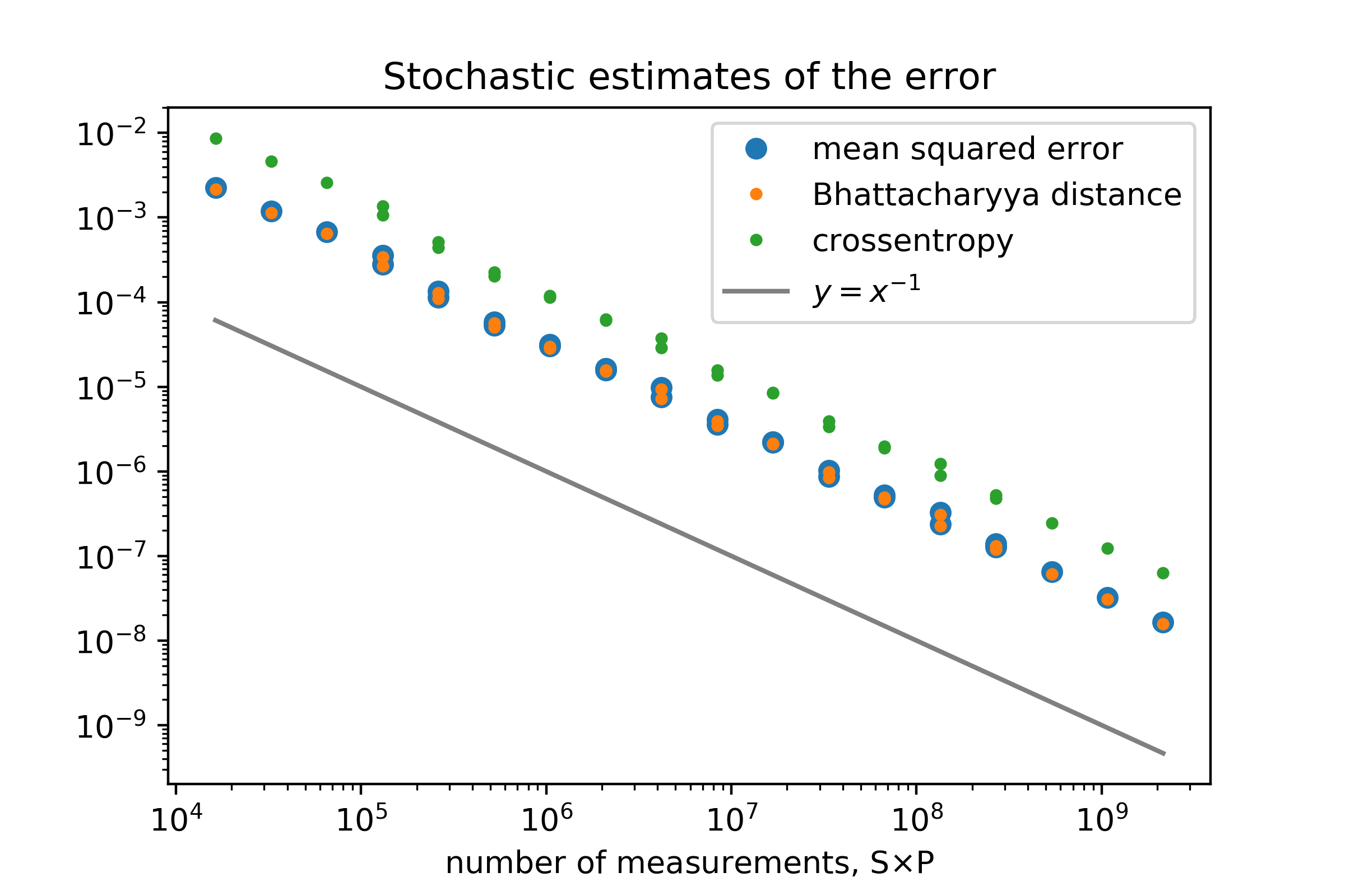
(a)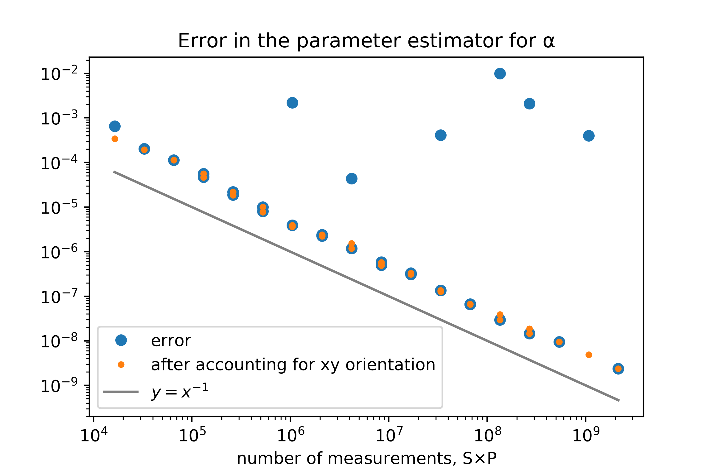 (b)
(b)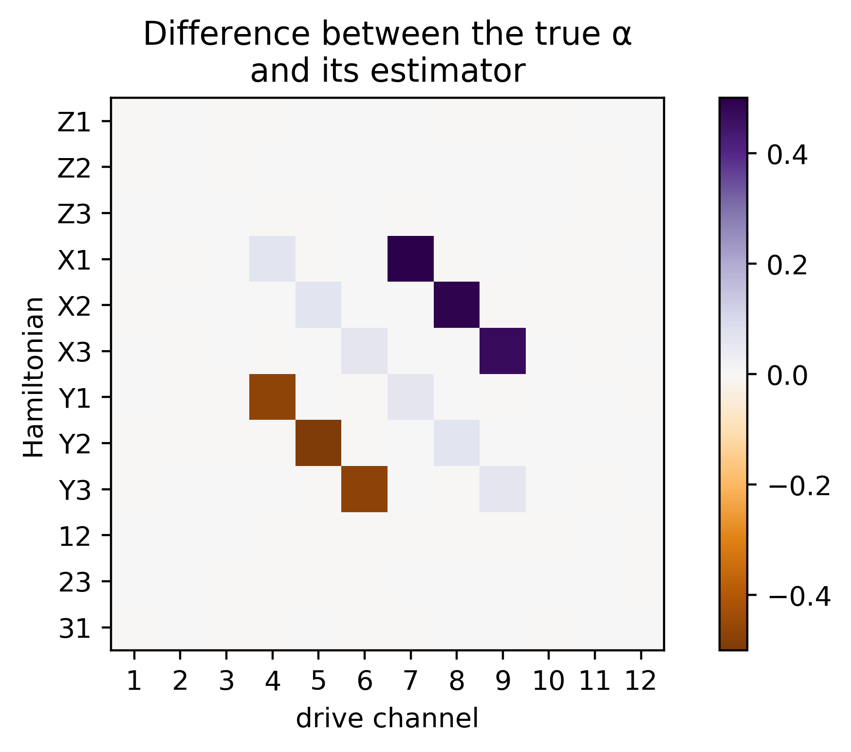 (c)
(c)
Our parameter estimation procedure is inherently stochastic, which is both a blessing and a curse. It is what permits us to use the entirety of the measurements performed on the hardware and reach the information-theoretic limits of precision. For numerical simplicity we choose a simple cost function—the mean squared error between measured and predicted populations—however we do observe consistent behavior independent of the particular choice of stochastic validation function (see Fig. 6a).
However, there might be a “gauge” degree of freedom in the way we have parameterized the Hamiltonian, which does not affect the actual dynamics of the system. As such, there might be parameters whose value will neither affect the measurement data we gather, nor will be of any consequence when designing control pulses down the road. Our choice of “indirect” validation function permits us to disregard this degree of freedom, as the validation function is sensitive only to the prediction of our model, not to the particular parameterization we have used in our model.
However, it would be instructive to observe how some of these “unimportant” parameters behave in our estimator. For instance, the test system used in much of this manuscript has a Hamiltonian of the form
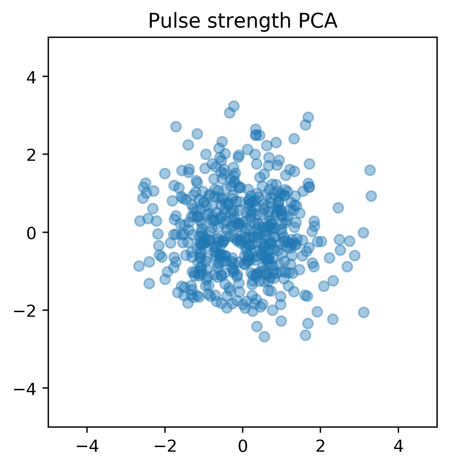
where denote the coupling strengths for each drive pulse component, and and are the strengths of Hamiltonian components that are present even in the absence of drives. Our estimator tries to model this Hamiltonian as , where and the set of possible is . We can see that the “true” is zero for the subset of operators , and the “true” is a diagonal matrix. However, in the measurement data used by the estimator, there is nothing that defines the orientation of the x axis in the xy plane. If we rotate all the qubits by the same angle around the z axis, the physics of the system (and the measured data) will not change. In other words, for this particular Hamiltonian, the change of xy basis generator commutes with the zero drive Hamiltonian , hence non-diagonal such as the one in Fig. 6c would predict the same evolution as the diagonal one.
In the case of a microwave superconducting circuit implementation, this freedom in the parameter would be due the fact that the master oscillator used in mixing the control signals has an arbitrary initial phase (this phase defines our choice of x and y axis in the rotating frame for all qubits).
More generally, as long as the random pulses we use in our stochastic cost function are representative of the pulses that will be used to control the hardware, such “gauge” degrees of freedom are inconsequential: if they do not affect our cost function, they will not affect the result of a computation running on the hardware either.
Appendix B The Choice of Cost Function, Estimator Efficiency, and the Cramér–Rao Bound
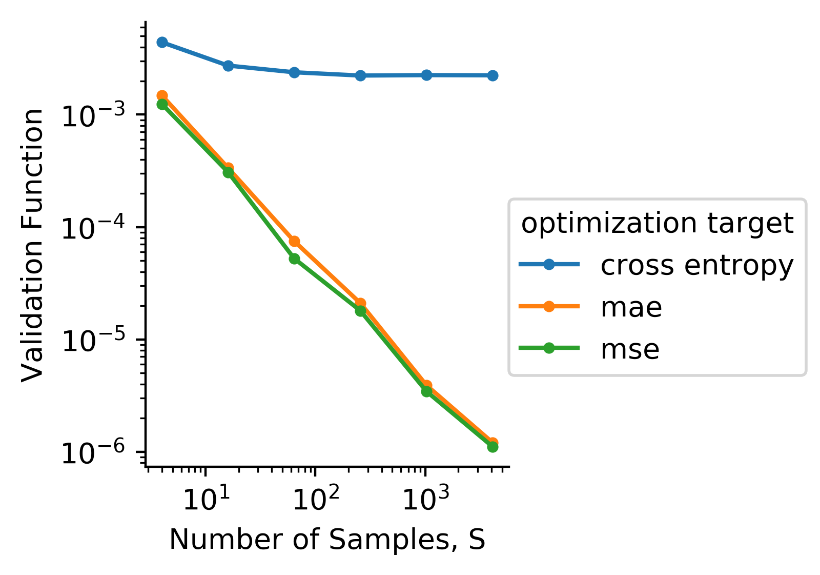
In the main text we invoked the Cramér–Rao bound in order to explain the fidelity scaling that we obtain in the case of unbiased estimation (before considering the effects of SPAM). That bound is a general information inequality that expresses a lower bound on the variance. Besides verifying numerically that we follow the bound (as done in the main text), it would be instructive to derive the variance of our particular estimator and compare it to this bound. This would help inform and defend our choice of , which until now has been based on computational convenience.
Let be the gradient of , and be the Hessian matrix. For our estimator we have where is our estimate for the true value . Expanding around we get
which leads us to
This permits us to estimate variances and covariances for the parameters
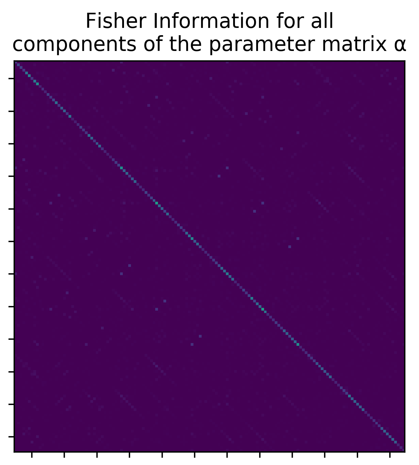
If we pick a maximal likelihood estimator (i.e. if the distance function is the cross entropy ), then we have and , where is the Fisher information matrix, therefore proving that we would saturate the Cramér–Rao bound and have a fully efficient estimator. In practice, one would need to consider the numerical stability of gradient descent as well: the estimator would be run with a number of different distance functions, to see empirically which one proves most reliable numerically. This led us to use the mean squared error in our examples, but other choices might be more performant in other settings (Fig. 7).
For completeness we also derive the explicit form of the Fisher information matrix used in arguments in the main text. First we denote the log-likelihood function
where is the predicted population in the -th state for the -th pulse in the training set and is the measured population for that state and pulse (by taking samples). This leads us to an expression for the Fisher information
where denotes average over all pulses in the training set. Also, happens to be the Fisher information for a single measurement of a single pulse, i.e. the Fisher information is additive.
Appendix C Convergence, Overfitting, and Model Errors
In the previous discussion we neglected issues of convergence, overfitting, and model errors. We use two complementary tools to fight these problems. Firstly, overfitting or being stuck in a valley of the cost function can both be avoided with an annealed regularization cost applied to the parameters.
The specific annealed and regularized cost function that we use as a function of iteration is of the form
where is given by Eq. 5 and the are annealed as increases, meaning that our estimator is essentially a LASSO-type estimator Tibshirani (1996).
From a purely practical point of view this avoids the initial steps of the gradient descent going in a wildly unphysical direction of pathological values for the parameters. More importantly, minimizing the 1-norm of the parameters provides for a sparser realistic parametrization. For particularly difficult programs we observed that empirical tricks akin to MacKay’s regularization annealing schedule (MacKay, 1992), where the variance in the regularization is forced to follow the variance in the cost enables reliable convergence.
The second tool involves extending the dynamics permitted in the model. Throughout the main text and in the following sections we discuss the biasing effect of various types of model errors (e.g. intrinsic SPAM not being included in the simplest models, or the effect of neglected parasitic couplings or other coherent errors in Fig. 8, or incoherent noise that can not be expressed in a Hamiltonian formalism). A quick fix solution we discussed is making the estimator more sensitive to parameter errors than to model errors by, e.g., using stronger pulses that accentuate the parameter errors. However, the more powerful solution, as long as it is computationally feasible, is to extend the model to include these otherwise neglected dynamics. Both of these approaches are described in the following sections.
Lastly, it is important to note the interaction between the regularization approach and the model extension approach. Permitting many more degrees of freedom in the model also leads to a higher risk of overfitting and convergence issues, hence leading to the need for annealed regularization. For particularly difficult problems one can even envision extending STEADY to a “hyper parameter” estimator where a discrete optimization algorithm evaluates a family of models by the Akaike information criterion (Akaike, 1974).
Appendix D Intrinsic SPAM
As described in the main text, we used the following model for the intrinsic state preparation error
and the following model for the measurement error: , where
and the only non-zero components of are where the Hamming distance between the binary representations of and is 1.
To find the bias in our estimator we will need to take a more careful look at the minimum of ( is what becomes in the presence of SPAM errors as described below). By definition of , that minimum will be at . For simplicity let us consider only measurement errors, which would cause the vector to become , where is an almost-diagonal stochastic matrix, with off-diagonal components on the order of , i.e. , where contains constant components on the order of unity. describes the chance that a measurement of a given state is wrongly reported as another state. While the state preparation errors are more complicated to express, because they happen before the dynamical evolution of the state, linearity guarantees that a similar treatment would work for an appropriately chosen ensemble of states. This leaves us with
Evaluated at it results in
where is a positive real number. Moreover, we have (because has its minimum at ) and (because has its minimum at ), where and are positive real numbers. Therefore
Given that we are interested in the regime where the bias overwhelms the statistical error, we can take the limit which results to leading order in , where is a positive real number. This leads to and the observed error floor of (see Fig. 3d).
This error floor is unsurmountable by simply increasing the number of acquired measurements. However, if we redo the expansion while keeping record of , we are left with . This immediately suggests a way to decrease the bias of our estimator: simply use longer (or more powerful) control pulses. Fig. 3c demonstrates the improvements due to this approach.
Appendix E Effects of Non-unitary Decay on Information Content
As we have seen in the rest of the manuscript, having an incomplete model, one that is incapable of expressing the entire dynamics, would cause bias in our estimator. This was observed both in the case of intrinsic SPAM, and in the case of Lindbladian dynamics. This issue can be addressed in some cases by making the estimator more sensitive to estimator errors (by using longer pulses). When this fails one can instead extend the model to include the missing dynamics. Both of these approaches were discussed in the main text.
However, the good performance of the Lindbladian model estimator from Fig. 5 can be counterintuitive. Taken to the extreme, strong decay would cause all of the information about the unitary evolution to leak out to the environment before the measurement. This extreme example seems to imply that the performance of the estimator should drop at extremely high decay parameters, which we do not observe. Similarly to the discussion in A, this stems from our choice of validation function; that is, we evaluate the quality of the predictions we can make about our system, and we do not evaluate directly how precise each parameter is estimated. Hence, when we are interested in the quality of predictions, we do not need to worry about parameters that do not affect the dynamics strongly. In the case of strong decays, all other parameters become unimportant, and this is why we do not see a drop in performance. The same phenomenon that makes parameters hard to estimate also makes them inconsequential to the dynamics of the system.
This can be observed in the Fisher information. Consider for simplicity a two level system. The excited state Born probability is in the case of unitary evolution. In the presence of decay, a first order approximation for that same probability is . The Fisher information with respect to for a single measurement is then , which in the limiting cases is and . Similarly, the Fisher information with respect to is , with limiting behavior and .
However, the validation function is to first order , where and are the true values of the parameters. Hence , where and are the variances in the estimators for each of the parameters (we neglect correlations). Due to the Cramér–Rao bound both variances scale as the inverse of the corresponding Fisher information, which leaves us with (see Fig. 9). Therefore, as the decay rate goes higher and leaves us with less and less available information per measurement, it also causes less diversity in the final measurements (high probability that the final state is the ground state), leading to small (“good”) values for the validation function. In practice, this effect becomes noticeable only at impractically high values for : while we do precisely predict in such cases how the state decays, this is not of particular use for devising control protocols for the system. Generally a system with strong decays is not particularly useful as a quantum hardware, unless we use “engineered dissipation” control schemes or control schemes employing virtual states like STIRAP (Unanyan et al., 1998), which are beyond the scope of this manuscript.
Appendix F Variance of Parameter Estimator in Linear Least Squares
Here we give a concrete analytical example of cases where the cost function has a floor dictated by , while the validation function has a floor dictated by . The description here is generic; it does not refer to a model of quantum dynamics.
The model we are learning is parameterized by . We denote by the pairs of (population estimate, pulse) that we are learning from (we have such pairs). For each pair we used repetitions in order to estimate , the population, for the given , the pulse.
The true population is (given that we are performing multinomial sampling, we approximate as drawn from a normal distribution with ).
We perform parameter estimation by minimizing least squares and the validation function is .
For the purpose of this example, consider linear least squares: the model we are fitting to has the parameters , and . and denote the parameter values which minimize . However, the data are governed by the “true” model .
The minimum of is reached at and , where:
-
•
a bar denotes the typical estimator of an average value;
-
•
;
-
•
denotes the estimator of the variance of ;
-
•
is the estimator of the covariance of and .
The estimated covariance can be calculated as,
Substituting the expressions for and in and factoring out the term leaves us with:
Hence the expectation value of is .
Appendix G Software Implementation
The estimators we implement are all fully differentiable programs, that can run “batches” of measurement data. They can run on both CPUs and GPUs, as well as any other optimized tensor processing units supported by Tensorflow, like Google’s TPU chips. The code is documented inline and extremely short (<50 lines of code per estimator). We implement the following estimators (all of them can be run either as stochastic parameter estimators where measurements are provided as training data, or as optimal control optimizers where the parameters are fixed but the control pulses are optimized for a given target).
-
•
StateProbabilitiesPaulied solves Schroedinger’s equation for
and where are fixed in advance. Control pulses for this solver are constant in time (with implied duration of ) provided as arrays of shape . The time-evolution operator is calculated through diagonalization of the Hamiltonian.
-
•
StateProbabilities solves Schroedinger’s equation for
with explicitly ensured Hermiticity (see the source code for details). Control pulses for this solver are constant in time (with implied duration of ) provided as arrays of shape . The time-evolution operator is calculated through diagonalization of the Hamiltonian.
-
•
Non-linear drives can be straightforwardly added to the above solvers by adding higher-order terms like , etc.
-
•
StateProbabilitiesTimeDep solves Schroedinger’s equation in either of the previous two forms, but for time dependent control pulses . Control pulses are piece-wise constant of implied total duration and a predetermined number of timesteps . The control pulses are provided as arrays of shape . The time evolution is computed through evaluating the consecutive time-evolution operators. Each operator is computed either, as above, through diagonalization, or through faster, but less precise, Taylor expansion of the matrix exponential (in Horner’s form).
-
•
StateProbabilitiesTimeDepLindblad solves Lindblad’s Master equation for time dependent control pulses . The Hamiltonian part is provided in either of the two forms discussed above. The control pulses are provided in the same format as above. The non-unitary evolution is modeled by fixed predetermined collapse operators , however the strengths of each collapse operator is a parameter optimized by the estimator. The full equation being modeled is
The integrator uses Euler’s method.
-
•
StateProbabilitiesTimeDepLindbladRK4 works as above but it uses the RK4 method for numerical integration.
-
•
Unlike gradients, Hessians do not permit fast backpropagation methods for their calculation (and hence are not well supported by differentiable programming frameworks yet). This led us to writing a simple numerical procedure for estimating the Hessians needed for the calculation of the Fisher information in AvgFIStateProbabilitiesPaulied. It is a proof-of-concept that works only on the first of the estimators described above, but it is the tool that permitted us to run experimental-design optimizations as described in the main text. It is implemented in a separate Jupyter notebook.
